| Issue |
A&A
Volume 645, January 2021
|
|
|---|---|---|
| Article Number | L7 | |
| Number of page(s) | 8 | |
| Section | Letters to the Editor | |
| DOI | https://doi.org/10.1051/0004-6361/202039546 | |
| Published online | 11 January 2021 | |
Letter to the Editor
Revisiting the progenitor of the low-luminosity type II-plateau supernova, SN 2008bk
1
Astrophysics Research Centre, School of Mathematics and Physics, Queen’s University Belfast, Belfast, BT7 1NN
UK
e-mail: This email address is being protected from spambots. You need JavaScript enabled to view it.
2
Department of Physics and Astronomy, University of Turku, Vesilinnantie 5, Turku, 20014
Finland
3
School of Physics, O’Brien Centre for Science North, University College Dublin, Belfield, Dublin 4, Ireland
4
Nicolaus Copernicus Astronomical Centre, Warsaw, Poland
5
Universidad de Concepción, Departamento de Astronomía, Concepción, Chile
6
Núcleo de Astronomía de la Facultad de Ingeniería y Ciencias, Universidad Diego Portales, Av. Ejército 441, Santiago, Chile
7
Millennium Institute of Astrophysics, Santiago, Chile
Received:
28
September
2020
Accepted:
26
November
2020
Abstract
The availability of updated model atmospheres for red supergiants and improvements in single and binary stellar evolution models, together with previously unpublished data, prompted us to revisit the progenitor of the low-luminosity type II-plateau supernova (type IIP SN), SN 2008bk. Using mid-infrared (mid-IR) data in combination with dust models, we find that high-temperature (4250−4500 K), high extinction (E(B − V)> 0.7) solutions are incompatible with the data. We therefore favour a cool (∼3500−3700 K) progenitor with a luminosity of log(L/L⊙) ∼ 4.53. Comparing with evolutionary tracks, we infer progenitor masses in the 8–10 M⊙ range in agreement with some previous studies. This mass is consistent with the observed pattern of low-luminosity type IIP SNe coming from the explosion of red supergiant stars (RSGs) at the lower extremum for core collapse. We also present multi-epoch data for the progenitor, but do not find clear evidence of variability.
Key words: stars: evolution / supernovae: general / supernovae: individual: 2008bk
© ESO 2021
1. Introduction
Although it is generally accepted that type II-plateau supernovae (IIP SNe) arise from the core collapse of red supergiant stars (RSGs), inferring the mass range of progenitors that give rise to type IIP SNe from observations remains challenging. The most direct way of detecting SN progenitors is by searching for them in archival pre-explosion imaging. This necessarily involves an element of serendipity, and although type IIP SNe are the most frequently occurring core-collapse subtype (Li et al. 2011), only 12 progenitors of type IIP/L SNe have been detected in this way to date; of these, only 7 have detections in more than two filters.
Poor wavelength coverage stemming from a lack of multi-band detections leads to a degeneracy between the inferred extinction and luminosity of the progenitor; these in turn result in large errors in the derived progenitor mass. At least two broadband colours sampling the optical to near-infrared (NIR) spectral energy distribution (SED) of the progenitor is a desirable prerequisite for such searches. Ideally, coverage of the SED of the progenitor from the ultraviolet (UV) through to the IR region would be available, but the bulk of archival data on hand are at optical wavelengths.
Summary of previous estimates for the properties of the progenitor star.
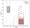 |
Fig. 2. Comparison between stellar evolution tracks and the allowed regions as inferred from the observations. Shown are the stellar evolution tracks of 8 ≤ MZAMS/M⊙ ≤ 14 for subsolar metallicity (log(Z/Z⊙) = − 0.4). The results from this study are depicted by boxes that show the allowed ranges in temperature and luminosity for the progenitor given the uncertainties. The grey and red shaded regions show the luminosity ranges estimated using the SEDs of the MARCS and PHOENIX models, respectively, and assuming the shorter (Cepheid and TRGB) distance of 3.5 ± 0.1 Mpc for our two best model matches (Sect. 3). The dashed lines extend the boxes to show the effect of considering the full distance range (3.32−4.32 Mpc). |
Early studies of directly detected progenitors found the zero-age main sequence mass (MZAMS) range of stars producing type II SNe to be  (Smartt et al. 2009, and references therein), the upper-mass end of which is markedly discrepant with theoretical expectations (e.g. 9 ≲ M⊙ ≲ 40, Heger et al. 2003). While the cause of this discrepancy is discussed frequently in the literature (e.g. Smartt 2015; Davies & Beasor 2018, 2020; Kochanek 2020), the lower mass limit is also of interest from an evolutionary standpoint. The (Fe) core collapse of low-mass RSGs is thought to give rise to low-luminosity IIP SNe, namely those with faint plateau magnitudes (−13.5 < MV < −16), low ejecta velocities (< 5000 km s−1
Pastorello et al. 2009), and 56Ni masses as low as ≲0.01 M⊙ (e.g. Chugai & Utrobin 2000). However, similar properties may also be due to the collapse of an O-Ne-Mg core in super-AGB stars with masses of ∼9 M⊙, giving rise to so-called electron-capture SNe (e.g. Poelarends et al. 2008; Pumo et al. 2009). Scenarios invoking higher mass RSGs have also been proposed for low-luminosity IIP SNe. These generally require a large amount of fallback to match the above properties (Zampieri et al. 2003; Nomoto et al. 2013). Reliably distinguishing between these possibilities remains one of the challenges of SN research.
(Smartt et al. 2009, and references therein), the upper-mass end of which is markedly discrepant with theoretical expectations (e.g. 9 ≲ M⊙ ≲ 40, Heger et al. 2003). While the cause of this discrepancy is discussed frequently in the literature (e.g. Smartt 2015; Davies & Beasor 2018, 2020; Kochanek 2020), the lower mass limit is also of interest from an evolutionary standpoint. The (Fe) core collapse of low-mass RSGs is thought to give rise to low-luminosity IIP SNe, namely those with faint plateau magnitudes (−13.5 < MV < −16), low ejecta velocities (< 5000 km s−1
Pastorello et al. 2009), and 56Ni masses as low as ≲0.01 M⊙ (e.g. Chugai & Utrobin 2000). However, similar properties may also be due to the collapse of an O-Ne-Mg core in super-AGB stars with masses of ∼9 M⊙, giving rise to so-called electron-capture SNe (e.g. Poelarends et al. 2008; Pumo et al. 2009). Scenarios invoking higher mass RSGs have also been proposed for low-luminosity IIP SNe. These generally require a large amount of fallback to match the above properties (Zampieri et al. 2003; Nomoto et al. 2013). Reliably distinguishing between these possibilities remains one of the challenges of SN research.
The low-luminosity and normal IIP SNe form a continuous distribution in brightness; here we simply adopt an upper brightness cut-off of Mvisual ∼ − 16. Although more than a dozen low-luminosity IIP SNe have been classified as such, only three have progenitor detections: SNe 2005cs, 2008bk, and 2018aoq (Maund et al. 2005; Li et al. 2006; Mattila et al. 2008; O’Neill et al. 2019), respectively. SN 2005cs occurred in M51 (8.4 Mpc); a progenitor was identified in archival Hubble Space Telescope (HST) images in only one filter (F814W). Combining this latter detection with upper limits from other filters, the progenitor mass was inferred to be 9 . SN 2018aoq occurred in NGC 4151 (18 Mpc). With progenitor detections in both optical (F350LP, F555W, and F814W), and NIR (F160W) HST filters, SN 2018aoq was estimated to have a mass of ∼10 M⊙ (O’Neill et al. 2019). SN 2008bk merits special attention as it occurred in NGC 7793 at a distance of only ∼3.5 Mpc (Pietrzyński et al. 2010; Zgirski et al. 2017). A wealth of pre-explosion archival data ranging from 3800−24000 Å are available, and the progenitor was clearly detected in multiple filters. A first analysis reported a progenitor mass of ∼8–9 M⊙ (Mattila et al. 2008; Van Dyk et al. 2012), which was later revised to ∼13 M⊙ (Maund et al. 2014), suggesting that higher mass RSGs could give rise to low-luminosity IIP SNe. Here we revisit this issue, motivated in part by updated model grids, and also by the existence of previously unpublished data for the progenitor.
Analysis of the progenitor of SN 2008bk by Mattila et al. (2008) and Van Dyk et al. (2012) showed that its SED could be fit by a MARCS (Gustafsson et al. 2008)1 model atmosphere with a temperature of ∼3500–3600 K. Despite differences in the photometry and adopted extinction values (E(B − V) = 0.32 and E(B − V) = 0.02, respectively), both studies infer a progenitor mass of 8.5 ± 1.0 M⊙ (Table 1).
Using late-time imaging, Mattila et al. (2010) found that the source previously identified as the progenitor had vanished, confirming its association with SN 2008bk. Using the photometry in Mattila et al. (2008), Davies et al. (2013) showed that a higher temperature of T = 4200 K and extinction E(B − V) = 0.67 also matched the progenitor SED.
Maund et al. (2014) noted that previous attempts to characterise the progenitor, especially from ground-based imaging, were probably affected by the combination of a crowded field and patchy background. These latter authors therefore obtained late-time template images using similar instrument and filter combinations as the pre-explosion imaging, allowing them to remove contaminating flux. Based on Bayesian fitting of the template-subtracted progenitor photometry to MARCS models, they inferred a temperature of 4330 K and E(B − V) = 0.77. This results in a significantly more luminous progenitor compared to previous studies, and a correspondingly more massive RSG of 12.9 M⊙ at the end of its He burning phase. Interestingly, the extinction towards field stars in the vicinity of SN 2008bk was found to be only E(B − V) = 0.09, leading Maund (2017) to conclude that their higher value must arise from CSM dust.
A recent study by Davies & Beasor (2018) favours a lower value of 8.3 ± 0.6 M⊙ on the grounds that RSGs evolve to later spectral types, and that this must be taken into consideration so that the appropriate bolometric correction can be applied.
Radiative transfer and hydrodynamical modelling of the photospheric and nebular phases of SN 2008bk allow for a 9–12 M⊙ progenitor (Lisakov et al. 2017; Jerkstrand et al. 2018; Martinez et al. 2020), thereby encompassing all previous progenitor mass estimates.
There are several estimates for the distance to 2008bk: a shorter 3.5 Mpc estimate derived from Cepheid variables and the tip of the red giant branch (TRGB; Pietrzyński et al. 2010; Jacobs et al. 2009 respectively), and a longer 3.9 Mpc estimate also via the TRGB (Karachentsev et al. 2003). Following Maund et al. (2014), we take the mean of the two more recent studies, which also favours the direct distance determination methods, that is, we adopt 3.5 ± 0.1 Mpc as the distance to the NGC 7793, unless stated otherwise (Table 1).
2. Methods
2.1. Archival data
Motivated by the discrepancy between the inferred temperature and mass for the progenitor, we report the results of a new analysis of the progenitor properties. For this, we used the late-time difference image photometry reported in Maund et al. (2014) as these measurements should suffer from minimal contamination in most filters. The pre-explosion images were taken across three epochs (2001, 2005, and 2007), while the templates are from 2011, using the same or similar instrumental setup. No templates free of SN emission were available for the g′ and r′ bands. The difference between the pre-explosion and template-subtracted images is < 0.2 mag for all filters except the i′ and I bands. For the latter, the progenitor is fainter in the difference images by ∼0.4 mag, suggesting field contamination.
We also present Spitzer/IRAC observations of the progenitor of SN 2008bk. Although there are two epochs of IRAC channels 1–4 pre-explosion imaging taken in 2004 by the SINGS programme (Table A.1), they are separated by only one day. All post-explosion data are from the warm Spitzer mission. As noted previously, the SN occurred in a relatively crowded region, and so template subtraction is a necessary step, especially given the IRAC pixel scale ( /pix).
We chose the 2018-04-06 epoch to use as a reference. This choice is arbitrary, because the post-explosion data are taken between 2014 and 2019, that is, long after the SN had faded. We checked that equivalent results were obtained by choosing a post-explosion epoch that was closest in orientation to the 2004 one. To carry out the subtraction, we used the post-basic calibrated data products. The image matching and subtraction was performed as implemented in the ISIS v2.2 image-subtraction package (Alard & Lupton 1998; Alard 2000). The pre- and post-explosion images, and the difference images for both channels are shown in Fig. A.1.
An aperture with a radius of 4 pixels was placed on the progenitor and its position was offset by 2-4 pixels in random directions around the progenitor position nine times to ensure that the aperture position does not strongly dictate the results. We applied the appropriate aperture corrections to the average value resulting from the above procedure, and converted to the Vega magnitude system.
Although no templates are available for channels 3 and 4, we can place limits on the progenitor brightness at these wavelengths. We note that there is no significant flux at the progenitor location (Fig. A.2). Van Dyk et al. (2012) also noted the lack of 8.0 μm (channel 4) emission, and attributed this to low extinction. In order to estimate the depth of these images, we constructed approximate point spread functions using field stars in the image. The brightness of these artificial sources was adjusted until they were detected at the 3σ level. The resulting photometry is given in Table A.1.
2.2. Spectral energy distribution fitting
In this study we use two different atmospheric model sets. The MARCS model grid used here is based on spherically symmetric calculations for a 15 M⊙ RSG star with surface gravities −0.5 ≤ log(g) ≤ + 1.0, metallicities −1.0 ≤ log(Z/Z⊙) ≤ + 0.5, and a temperature range of 3300–4500 K, with a step size of 100 K for models below 4000 K and 250 K for those above this value.
The PHOENIX models (Lançon et al. 2007) are also spherically symmetric and are part of the STSYNPHOT python package, which allows us to easily generate SEDs with a wide range of temperatures, metallicities, and surface gravities. Here we adopt the same temperature range as for the MARCS models (3300–4500 K), with a step size of 100 K.
Many previous studies have pointed out that it is difficult to accurately capture the physical processes occurring in the outer layers of RSGs without computationally expensive detailed 3D hydrodynamical modelling (e.g. Chiavassa et al. 2009). Nevertheless, the grids of 1D spherically symmetric models computed under the assumption of local thermodynamic equilibrium have been shown to be in good general agreement with the optical–infrared SEDs (e.g. Levesque et al. 2005; Davies et al. 2013)
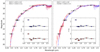 |
Fig. 1. Left: comparison between the two best fitting MARCS models. Black points mark the photometric points from the progenitor. The horizontal uncertainties simply denote the width of the photometric band. Inset are the residuals between the photometry and the SEDs for both fits. We note the large disagreement between the SEDs and the g′ band point at 0.46 μm. Right: comparison between the high temperature, high extinction MARCS model and the best fitting PHOENIX model. The PHOENIX model appears to fit the blue g′ band much better, however it overestimates the flux in the optical >6500 Å. The mid-IR points (Table A.1) are not shown here for clarity and ease of comparison with previous studies. |
Using a Monte-Carlo weighted fitting technique we attempted to match the model SEDs to the progenitor photometry. The initial fitting parameters were temperature, luminosity, and line-of-sight extinction, for which we adopted RV = 3.1, and circumstellar medium (CSM) extinction, for which we use the equations in Kochanek et al. (2012). We set a lower bound for the former, corresponding to the line-of-sight Milky Way contribution of E(B − V) = 0.02 mag (Schlafly & Finkbeiner 2011). We only considered models with a surface gravity value of log(g) = 0.0. All previous studies found that the metallicity of the progenitor environment was most likely sub-solar (see Table 1), and so we adopted models computed with a metallicity closest to previously reported values, namely log(Z/Z⊙) = − 0.25.
The temperature, luminosity, and extinction parameters were sampled from a normal distribution with an initial central value; the initial temperature was set to 3900 K, the initial brightness to mr′ = 22 mag, the line-of-sight extinction E(B − V) = 0.3 mag, and the optical depth of the CSM τV = 1 and is allowed to vary in the range 0 ≤ τv ≤ 20. We set the distributions to be wide enough to allow the entire range of parameters to be sampled. We then constructed SEDs from a randomly selected combination of temperature, luminosity, and extinction values, and computed the scatter between synthetic and observed magnitudes. If the scatter decreased compared to the previous best-fitting iteration, the central values of the distribution were shifted to these, and the process repeated with the sampling width slowly narrowing if no improved fits are found. In effect, this results in the sampling distributions becoming narrower while moving through the parameter space. This process was carried out for 10 000 iterations with the parameters producing the best-fitting SED returned at the end of the process. The width of the sampling function at the end of this process is taken to be the resulting uncertainty provided that it is larger than the grid step size.
3. Results and discussion
For the MARCS models, we find two combinations of parameters that match the observed SED. The first results in a scatter δmag = 0.14 mag, and is a 3500 ± 150 K model with minimal extinction E(B − V) ≈ 0.02, similar to Mattila et al. (2008) and Van Dyk et al. (2012). However, a similar match (δmag = 0.15 mag) is obtained with a 4500 ± 250 K model with a relatively high extinction of E(B − V) = 0.88, which echoes the result reported by Maund et al. (2014). The SEDs and residuals for both models are shown in the left-hand panel of Fig. 1.
While both SEDs match the majority of the optical and NIR data points, there is a very large discrepancy between the SED of either model and the g′ band magnitude (λc = 0.46μm), resulting in a large (∼1 mag) residual as shown in the inset panel of Fig. 1. As mentioned previously, the g′ band magnitude may well be contaminated by nearby unrelated sources. However, it is difficult to attribute such a large discrepancy solely to contamination because the r′ band point –which also lacks a template– is consistent with the model SED, implying that any contaminating source would emit predominantly at bluer wavelengths. We find no significant difference between SEDs with and without CSM extinction. However, we note that there is some degeneracy between the line of sight and CSM extinction, in the sense that while the total visual extinction remains the same, the relative contribution of the components changes.
We can infer the luminosity of the progenitor by correcting for extinction and integrating over the model SEDs. By comparing these results with STARS stellar evolution tracks (Eggleton et al. 2011), we can estimate the mass of such a star. For the hotter MARCS model, we find a luminosity of  but no clear match to any stellar evolution tracks. For the lower temperature one, we find a luminosity of
  which is consistent with the evolution of 8–9 M⊙ stars. The region also includes the point at which the lowest mass (8 M⊙) model terminates (see Table 1). Barring uncertainties in the models, we also consider the effect of allowing a larger error in the distance estimate (Fig. 2).
For the PHOENIX models, we find the best match (δmag = 0.06 mag) with a T = 3500 ± 160 K model and extinction E(B − V) = 0.07, corresponding to  , and matching the end-point luminosity of an 8 M⊙ track. We examined the impact of changing the metallicity to log(Z/Z⊙) = − 0.5 and 0.0 for both MARCS and PHOENIX models, and found results that are consistent with the above.
We also compared our results to the BPASS binary stellar evolution models (Eldridge et al. 2017). For the lower temperature MARCS and PHOENIX models, we find two groups of binary models that match. The majority consist of an 8.5 M⊙ star in a long-period orbit (log(Pdays) ≳ 3) that undergoes little or no interaction with its companion, essentially evolving as a single star. The second grouping consists of mergers of lower mass stars with combined masses in the 6−9 M⊙ range. We are unable to find any matches with the higher temperature models. We can rule out the former given that no source was detected in deep late-time imaging (Mattila et al. 2010; Maund et al. 2014).
As can be seen in the right-hand panel of Fig. 1, the scatter of the PHOENIX model is smaller (δmag = 0.06) compared to that of the MARCS models. In particular, the match to the g′ band point is significantly better, although there is a small excess in the range of 0.75–1.5 μm that is not apparent in the MARCS models. Previous studies on RSGs also noted a disagreement between MARCS and PHOENIX models at bluer wavelengths, such as for example Plez (2011) who noted a large (< 0.25 mag) difference for the U − B colour for Teff < 4000 K. Given the complexity of these models, the source of this discrepancy remains to be securely identified.
Many studies have noted the tension between the extinction inferred from SED fitting for example and that expected from studies of known RSGs (e.g. Kochanek et al. 2012; Walmswell & Eldridge 2012). Taken at face value, our findings support an 8–9 M⊙ progenitor.
However, detailed modelling of the SN allows a wider range of ∼9−12 M⊙, suggesting that it may only be possible to distinguish between these alternatives following improvements in the input physics of stellar evolution codes.
The low extinction value for our cooler model appears to be at odds with the values typically inferred for RSGs (e.g. Davies et al. 2013). One possibility is that the complexities of the dust properties are not wholly captured by the methods used above. Interestingly, most previous studies that report RSG progenitors of type IIP SNe also report extinctions that are significantly lower compared to RSGs, but the extinction values are often inferred from SN observations that obviously cannot constrain progenitor CSM dust properties, and indeed some or all of the pre-existing dust may be destroyed by the explosion.
We are therefore faced with a choice of either accepting our cooler model, or making use of the common knowledge of the properties of RSGs, and insisting that the higher extinction solution is preferable. However, there is a further test that we can carry out: we can check whether the mid-IR photometry is consistent with the high-extinction case, in the knowledge that RSGs are strong emitters at these wavelengths. In order to do so, we used the DUSTY code (Ivezic et al. 1999) using the same parameters as in Kochanek et al. (2012), that is, 50/50 silicate and graphite dust in a shell with radius Rin/Rout = 2, and a dust temperature of TD=1000 K. We then applied this formulation of the CSM reddening to MARCS models with temperatures 3300−4500 K that had been previously reddened only with a line-of-sight component of E(B − V) = 0.05.
We then used a Markov chain Monte Carlo fitting algorithm (python package emcee, Foreman-Mackey et al. 2013) to determine the most likely temperature, CSM dust extinction, and luminosity parameters based on the 0.6−8 μm SED. In keeping with Maund et al. (2014), we did not include the g-band point in the fit (see also Fig. 1). We find a solution with  K, and
  that is a good match to the progenitor SED.
A clear outcome is that when the dust emission is accounted for, the measured mid-IR magnitudes are significantly fainter than expected for a source with τv ∼ 2−3. High-temperature models with low CSM extinction are much too blue, while those with high extinction are much too bright in the mid-IR. These outcomes are depicted in Fig. 3. This exercise therefore favours a cool (T = 3500−3700 K), low-extinction source. We verified that this outcome is robust against variations in dust composition and temperature.
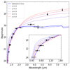 |
Fig. 3. Output from the DUSTY models showing the hotter (T = 4500 K) MARCS model with various amounts of CSM reddening (dashed lines) scaled to match the H and Ks bands. Also shown is the best fitting, cooler (T = 3500 K, E(B − V) = 0.02) model (solid line). Both have been re-binned to match the wavelength grid of the DUSTY models. The inset shows zoomed-in view of the optical region only; the open circle denotes the g-band point. It is immediately apparent that the mid-IR data are only consistent with low extinction. The low-extinction, high-temperature SED is too blue and does not match the optical data, while the high-extinction, high-temperature SED results in mid-IR emission that is too bright compared to the data. |
4. Progenitor variability
Many previous studies have remarked upon an apparent temporal coincidence between eruptive mass loss and core collapse, especially within the context of interacting (type IIn) SNe (e.g. Smith 2014). Such a correlation is difficult to observe given the inherent biases resulting from gaps in the data and the depths of previous and current transient surveys. From a theoretical point of view, a number of processes have been identified that could give rise to outbursts prior to core collapse (Quataert & Shiode 2012; Smith & Arnett 2014), but it is not yet clear which of these processes, if any, occur in reality and have observable consequences.
Kochanek et al. (2017) and Johnson et al. (2018) discuss this specifically for the case of RSGs. Only four type IIP SN progenitors have multi-epoch observations: SNe 2013ej (5 epochs over 5 years, Fraser et al. 2014), 2016cok (15 epochs over 8 years, Kochanek et al. 2017), and 2018aoq (9 epochs over 1 year, O’Neill et al. 2019), were observed in multiple optical HST filters with the progenitor of 2018aoq also having very limited HST NIR data. The progenitor of 2017eaw has limited observations in the optical filters, but has an extensive mid-IR coverage (34 epochs over 13 years, Kilpatrick & Foley 2018). Interestingly, none of these objects displayed significant variability within the diverse time-spans and cadences of the available datasets. The field of NGC 7793 containing SN 2008bk was repeatedly imaged as a part of Araucaria project (Gieren et al. 2005) with the 1.3m Warsaw telescope (Udalski et al. 1992). There are two sets of observations starting in mid-2004 that span 15 months in total, separated by ∼200 d.
Figure A.3 shows the I-band light curve of the progenitor analysed in the present study. The average magnitude over the total time-span of the observations is mI = 20.88 ± 0.11, which is ∼0.38 mag brighter than that reported by Maund et al. (2014).
In the first group of observations from MJD = 3250–3260, the source displays no significant variability (ΔmI ≤ 0.1 mag), apart from a single epoch at MJD = 3314.7 (mI = 21.13 ± 0.19) that is marginally consistent with the above average value. However, in the second set of observations (MJD = 3615.7–3712.5), there appears to be a drop in brightness within the range MJD = 3684–3685 of ∼0.6 mag from mI ∼ 20.8 ± 0.13 to ∼21.4 ± 0.24 mag.
We find that there are two points that deviate from the mean value at the 3σ level. For a sample of 39 points, we would expect to observe none. Given the associated measurement uncertainties, and the apparent rapidity of the fluctuations, intrinsic source variability is at best tentative. Although our dataset does not formally permit us to invoke variability, we note that periodic and stochastic variability is a hallmark of RSGs, which is in some cases also accompanied by changes in temperature and local extinction (e.g. Massey et al. 2007; Montargès 2020).
As mentioned above, the low extinctions reported for the progenitors of other IIP SNe are at odds with most RSG observations. We speculate that if a large fraction of the IIP SNe with known progenitors arise from mergers (Zapartas et al. 2017), then it is likely that any CSM dust will be destroyed or dissipated in this process. Whether or not the merger product subsequently produces large quantities of dust in spite of the dramatic alteration of its interior chemical profile is a matter that remains to be investigated.
Model Atmospheres in Radiative and Convective Scheme; https://marcs.astro.uu.se/index.php
Acknowledgments
D. O’Neill acknowledges a DEL studentship award and FINCA for supporting a research visit. MF is supported by a Royal Society - Science Foundation Ireland University Research Fellowship. Support for JLP is provided in part by FONDECYT through the grant 1191038 and by ANID’s Millennium Science Initiative through grant IC12_009, awarded to The Millennium Institute of Astrophysics, MAS. The research leading to these results has received funding from the European Research Council (ERC) under the European Union’s Horizon 2020 research and innovation programme under grant agreement No 695099 (project CepBin).
References
- Alard, C. 2000, A&AS, 144, 363 [NASA ADS] [CrossRef] [EDP Sciences] [Google Scholar]
- Alard, C., & Lupton, R. H. 1998, ApJ, 503, 325 [NASA ADS] [CrossRef] [Google Scholar]
- Chiavassa, A., Plez, B., Josselin, E., & Freytag, B. 2009, A&A, 506, 1351 [NASA ADS] [CrossRef] [EDP Sciences] [MathSciNet] [Google Scholar]
- Chugai, N. N., & Utrobin, V. P. 2000, A&A, 354, 557 [NASA ADS] [Google Scholar]
- Davies, B., & Beasor, E. R. 2018, MNRAS, 474, 2116 [Google Scholar]
- Davies, B., & Beasor, E. R. 2020, MNRAS, 493, 468 [NASA ADS] [CrossRef] [Google Scholar]
- Davies, B., Kudritzki, R.-P., Plez, B., et al. 2013, ApJ, 767, 3 [NASA ADS] [CrossRef] [Google Scholar]
- Eggleton, P. P., Tout, C., Pols, O., et al. 2011, STARS: A Stellar Evolution Code (Astrophysics Source Code Library) [Google Scholar]
- Eldridge, J. J., Stanway, E. R., Xiao, L., et al. 2017, PASA, 34, e058 [NASA ADS] [CrossRef] [Google Scholar]
- Foreman-Mackey, D., Hogg, D. W., Lang, D., & Goodman, J. 2013, PASP, 125, 306 [Google Scholar]
- Fraser, M., Maund, J. R., Smartt, S. J., et al. 2014, MNRAS, 439, L56 [NASA ADS] [CrossRef] [Google Scholar]
- Gieren, W., Pietrzynski, G., Bresolin, F., et al. 2005, Messenger, 121, 23 [Google Scholar]
- Gustafsson, B., Edvardsson, B., Eriksson, K., et al. 2008, A&A, 486, 951 [NASA ADS] [CrossRef] [EDP Sciences] [Google Scholar]
- Heger, A., Fryer, C. L., Woosley, S. E., Langer, N., & Hartmann, D. H. 2003, ApJ, 591, 288 [NASA ADS] [CrossRef] [Google Scholar]
- Ivezic, Z., Nenkova, M., & Elitzur, M. 1999, ArXiv e-prints [arXiv:astro-ph/9910475] [Google Scholar]
- Jacobs, B. A., Rizzi, L., Tully, R. B., et al. 2009, AJ, 138, 332 [NASA ADS] [CrossRef] [MathSciNet] [Google Scholar]
- Jerkstrand, A., Ertl, T., Janka, H. T., et al. 2018, MNRAS, 475, 277 [NASA ADS] [CrossRef] [Google Scholar]
- Johnson, S. A., Kochanek, C. S., & Adams, S. M. 2018, MNRAS, 480, 1696 [NASA ADS] [Google Scholar]
- Karachentsev, I. D., Grebel, E. K., Sharina, M. E., et al. 2003, A&A, 404, 93 [NASA ADS] [CrossRef] [EDP Sciences] [Google Scholar]
- Kilpatrick, C. D., & Foley, R. J. 2018, MNRAS, 481, 2536 [NASA ADS] [CrossRef] [Google Scholar]
- Kochanek, C. S. 2020, MNRAS, 493, 4945 [CrossRef] [Google Scholar]
- Kochanek, C. S., Khan, R., & Dai, X. 2012, ApJ, 759, 20 [NASA ADS] [CrossRef] [Google Scholar]
- Kochanek, C. S., Fraser, M., Adams, S. M., et al. 2017, MNRAS, 467, 3347 [NASA ADS] [CrossRef] [Google Scholar]
- Lançon, A., Hauschildt, P. H., Ladjal, D., & Mouhcine, M. 2007, A&A, 468, 205 [NASA ADS] [CrossRef] [EDP Sciences] [Google Scholar]
- Levesque, E. M., Massey, P., Olsen, K. A. G., et al. 2005, ApJ, 628, 973 [NASA ADS] [CrossRef] [Google Scholar]
- Li, W., Van Dyk, S. D., Filippenko, A. V., et al. 2006, ApJ, 641, 1060 [NASA ADS] [CrossRef] [Google Scholar]
- Li, W., Leaman, J., Chornock, R., et al. 2011, MNRAS, 412, 1441 [NASA ADS] [CrossRef] [Google Scholar]
- Lisakov, S. M., Dessart, L., Hillier, D. J., Waldman, R., & Livne, E. 2017, MNRAS, 466, 34 [NASA ADS] [CrossRef] [Google Scholar]
- Martinez, L., Bersten, M. C., Anderson, J. P., et al. 2020, A&A, 642 [Google Scholar]
- Massey, P., Levesque, E. M., Olsen, K. A. G., Plez, B., & Skiff, B. A. 2007, ApJ, 660, 301 [NASA ADS] [CrossRef] [Google Scholar]
- Mattila, S., Smartt, S. J., Eldridge, J. J., et al. 2008, ApJ, 688, L91 [NASA ADS] [CrossRef] [Google Scholar]
- Mattila, S., Smartt, S., Maund, J., Benetti, S., & Ergon, M. 2010, ArXiv e-prints [arXiv:1011.5494] [Google Scholar]
- Maund, J. R. 2017, MNRAS, 469, 2202 [NASA ADS] [CrossRef] [Google Scholar]
- Maund, J. R., Smartt, S. J., & Danziger, I. J. 2005, MNRAS, 364, L33 [NASA ADS] [CrossRef] [Google Scholar]
- Maund, J. R., Mattila, S., Ramirez-Ruiz, E., & Eldridge, J. J. 2014, MNRAS, 438, 1577 [NASA ADS] [CrossRef] [Google Scholar]
- Montargès, M. 2020, https://www.eso.org/public/news/eso2003/ [Google Scholar]
- Nomoto, K., Kobayashi, C., & Tominaga, N. 2013, ARA&A, 51, 457 [NASA ADS] [CrossRef] [Google Scholar]
- O’Neill, D., Kotak, R., Fraser, M., et al. 2019, A&A, 622, L1 [NASA ADS] [CrossRef] [EDP Sciences] [Google Scholar]
- Pastorello, A., Valenti, S., Zampieri, L., et al. 2009, MNRAS, 394, 2266 [NASA ADS] [CrossRef] [Google Scholar]
- Pietrzyński, G., Gieren, W., Hamuy, M., et al. 2010, AJ, 140, 1475 [NASA ADS] [CrossRef] [Google Scholar]
- Plez, B. 2011, J. Phys. Conf. Ser., 328, 012005 [Google Scholar]
- Poelarends, A. J. T., Herwig, F., Langer, N., & Heger, A. 2008, ApJ, 675, 614 [NASA ADS] [CrossRef] [Google Scholar]
- Pumo, M. L., Turatto, M., Botticella, M. T., et al. 2009, ApJ, 705, L138 [NASA ADS] [CrossRef] [Google Scholar]
- Quataert, E., & Shiode, J. 2012, MNRAS, 423, L92 [NASA ADS] [CrossRef] [Google Scholar]
- Schlafly, E. F., & Finkbeiner, D. P. 2011, ApJ, 737, 103 [NASA ADS] [CrossRef] [Google Scholar]
- Smartt, S. J. 2015, PASA, 32, e016 [NASA ADS] [CrossRef] [Google Scholar]
- Smartt, S. J., Eldridge, J. J., Crockett, R. M., & Maund, J. R. 2009, MNRAS, 395, 1409 [NASA ADS] [CrossRef] [Google Scholar]
- Smith, N. 2014, ARA&A, 52, 487 [NASA ADS] [CrossRef] [MathSciNet] [Google Scholar]
- Smith, N., & Arnett, W. D. 2014, ApJ, 785, 82 [NASA ADS] [CrossRef] [Google Scholar]
- Udalski, A., Szymanski, M., Kaluzny, J., Kubiak, M., & Mateo, M. 1992, Acta Astron., 42, 253 [NASA ADS] [Google Scholar]
- Van Dyk, S. D., Davidge, T. J., Elias-Rosa, N., et al. 2012, AJ, 143, 19 [NASA ADS] [CrossRef] [Google Scholar]
- Walmswell, J. J., & Eldridge, J. J. 2012, MNRAS, 419, 2054 [NASA ADS] [CrossRef] [Google Scholar]
- Zampieri, L., Pastorello, A., Turatto, M., et al. 2003, MNRAS, 338, 711 [NASA ADS] [CrossRef] [Google Scholar]
- Zapartas, E., de Mink, S. E., Izzard, R. G., et al. 2017, A&A, 601, A29 [NASA ADS] [CrossRef] [EDP Sciences] [Google Scholar]
- Zgirski, B., Gieren, W., Pietrzyński, G., et al. 2017, ApJ, 847, 88 [NASA ADS] [CrossRef] [Google Scholar]
Appendix A: Additional figures and tables
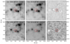 |
Fig. A.1. NIR IRAC images showing the detection of the progenitor. Left: pre-SN images showing the progenitor (red) circle in channels 1 (top) and 2 (bottom). Middle: post-explosion images in channels 1 and 2. Right: difference images (post-explosion − pre-explosion image). There is a source visible at the progenitor position in both channels. We detect it with an S/N of ∼10 (≫3σ) in channel 1, and an S/N of ∼4 (∼3σ) in channel 2. |
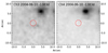 |
Fig. A.2. Pre-explosion images showing the progenitor position (red circle) in IRAC channels 3 (left) and 4 (right). Upper limits on the flux at this location are given in Table A.1. |
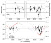 |
Fig. A.3. I band light curve of the progenitor of SN 2008bk. Top: the solid line denotes the weighted mean average magnitude for the dataset. The dashed lines represent the 3σ variation for the dataset. The values have only been corrected for Milky Way reddening. The vertical line shows the epochs at which the IRAC data were observed. Bottom: light curve of the progenitor alongside the light curves of three other RSG stars. The α Ori V-band light curve data were obtained from AAVSO (https://www.aavso.org/) while the V-band data for the LMC RSGs are from ASAS (http://www.astrouw.edu.pl/asas/?page=main). There are limited I-band data for the objects. The brightnesses of the sample RSGs are scaled such that the mean magnitude over the dataset is the same as that of the progenitor; they are also shifted in time such that the minimum in the light curve matches that of the progenitor. The progenitor of SN 2008bk does not show the slow variations displayed by well-known Galactic and other LMC RSGs. |
Summary of the pre-explosion IRAC data used in this paper.
OGLE I-band data.
All Tables
All Figures
|
Fig. 2. Comparison between stellar evolution tracks and the allowed regions as inferred from the observations. Shown are the stellar evolution tracks of 8 ≤ MZAMS/M⊙ ≤ 14 for subsolar metallicity (log(Z/Z⊙) = − 0.4). The results from this study are depicted by boxes that show the allowed ranges in temperature and luminosity for the progenitor given the uncertainties. The grey and red shaded regions show the luminosity ranges estimated using the SEDs of the MARCS and PHOENIX models, respectively, and assuming the shorter (Cepheid and TRGB) distance of 3.5 ± 0.1 Mpc for our two best model matches (Sect. 3). The dashed lines extend the boxes to show the effect of considering the full distance range (3.32−4.32 Mpc). |
| In the text | |
|
Fig. 1. Left: comparison between the two best fitting MARCS models. Black points mark the photometric points from the progenitor. The horizontal uncertainties simply denote the width of the photometric band. Inset are the residuals between the photometry and the SEDs for both fits. We note the large disagreement between the SEDs and the g′ band point at 0.46 μm. Right: comparison between the high temperature, high extinction MARCS model and the best fitting PHOENIX model. The PHOENIX model appears to fit the blue g′ band much better, however it overestimates the flux in the optical >6500 Å. The mid-IR points (Table A.1) are not shown here for clarity and ease of comparison with previous studies. |
| In the text | |
|
Fig. 3. Output from the DUSTY models showing the hotter (T = 4500 K) MARCS model with various amounts of CSM reddening (dashed lines) scaled to match the H and Ks bands. Also shown is the best fitting, cooler (T = 3500 K, E(B − V) = 0.02) model (solid line). Both have been re-binned to match the wavelength grid of the DUSTY models. The inset shows zoomed-in view of the optical region only; the open circle denotes the g-band point. It is immediately apparent that the mid-IR data are only consistent with low extinction. The low-extinction, high-temperature SED is too blue and does not match the optical data, while the high-extinction, high-temperature SED results in mid-IR emission that is too bright compared to the data. |
| In the text | |
|
Fig. A.1. NIR IRAC images showing the detection of the progenitor. Left: pre-SN images showing the progenitor (red) circle in channels 1 (top) and 2 (bottom). Middle: post-explosion images in channels 1 and 2. Right: difference images (post-explosion − pre-explosion image). There is a source visible at the progenitor position in both channels. We detect it with an S/N of ∼10 (≫3σ) in channel 1, and an S/N of ∼4 (∼3σ) in channel 2. |
| In the text | |
|
Fig. A.2. Pre-explosion images showing the progenitor position (red circle) in IRAC channels 3 (left) and 4 (right). Upper limits on the flux at this location are given in Table A.1. |
| In the text | |
|
Fig. A.3. I band light curve of the progenitor of SN 2008bk. Top: the solid line denotes the weighted mean average magnitude for the dataset. The dashed lines represent the 3σ variation for the dataset. The values have only been corrected for Milky Way reddening. The vertical line shows the epochs at which the IRAC data were observed. Bottom: light curve of the progenitor alongside the light curves of three other RSG stars. The α Ori V-band light curve data were obtained from AAVSO (https://www.aavso.org/) while the V-band data for the LMC RSGs are from ASAS (http://www.astrouw.edu.pl/asas/?page=main). There are limited I-band data for the objects. The brightnesses of the sample RSGs are scaled such that the mean magnitude over the dataset is the same as that of the progenitor; they are also shifted in time such that the minimum in the light curve matches that of the progenitor. The progenitor of SN 2008bk does not show the slow variations displayed by well-known Galactic and other LMC RSGs. |
| In the text | |
Current usage metrics show cumulative count of Article Views (full-text article views including HTML views, PDF and ePub downloads, according to the available data) and Abstracts Views on Vision4Press platform.
Data correspond to usage on the plateform after 2015. The current usage metrics is available 48-96 hours after online publication and is updated daily on week days.
Initial download of the metrics may take a while.