| Issue |
A&A
Volume 694, February 2025
|
|
|---|---|---|
| Article Number | A260 | |
| Number of page(s) | 18 | |
| Section | Extragalactic astronomy | |
| DOI | https://doi.org/10.1051/0004-6361/202452507 | |
| Published online | 19 February 2025 | |
SN 2018is: A low-luminosity Type IIP supernova with narrow hydrogen emission lines at early phases
1
Instituto de Astrofísica, Universidad Andres Bello, Fernandez Concha 700, Las Condes, Santiago RM, Chile
2
Millennium Institute of Astrophysics (MAS), Nuncio Monsenor Sòtero Sanz 100, Providencia, Santiago RM, Chile
3
Aryabhatta Research Institute of observational sciencES, Manora Peak, Nainital 263001, India
4
Department of Physics and Astronomy, University of California, Davis, 1 Shields Avenue, Davis, CA 95616-5270, USA
5
Steward Observatory, University of Arizona, 933 North Cherry Avenue, Tucson, AZ 85721-0065, USA
6
INAF Osservatorio Astronomico di Padova, Vicolo dell’Osservatorio 5, I-35122 Padova, Italy
7
INAF Osservatorio Astronomico di Brera, Via E. Bianchi 46, I-23807 Merate (LC), Italy
8
Instituto de Alta Investigación, Universidad de Tarapacá, Casilla 7D, Arica, Chile
9
Department of Physics and Astronomy, Aarhus University, Ny Munkegade 120, DK-8000 Aarhus C, Denmark
10
Department of Astronomy, The Oskar Klein Center, Stockholm University, AlbaNova, 106 91 Stockholm, Sweden
11
Indian Institute of Astrophysics, Koramangala 2nd Block, Bangalore 560034, India
12
Gemini Observatory, 670 North A’ohoku Place, Hilo, HI 96720-2700, USA
13
The School of Physics and Astronomy, Tel Aviv University, Tel Aviv 69978, Israel
14
CIFAR Azrieli Global Scholars program, CIFAR, Toronto, ON M5G 1M1, Canada
15
Institute for Astronomy, University of Hawai’i at Manoa, 2680 Woodlawn Dr., Hawai’i, HI 96822, USA
16
Department of Physics, Virginia Tech, Blacksburg, VA 24061, USA
17
South African Astronomical Observatory, PO Box 9 Observatory 7935, Cape Town, South Africa
18
Department of Astronomy, University of Cape Town, Private Bag X3, Rondebosch 7701, South Africa
19
Department of Physics, University of the Free State, P.O. Box 339 Bloemfontein 9300, South Africa
20
SURF, Science Park 140, 1098 XG Amsterdam, The Netherlands
21
Department of Physics and Astronomy, Michigan State University, 567 Wilson Road, East Lansing, MI 48824, USA
22
European Southern Observatory, Alonso de C’ordova 3107, Casilla 19, Santiago 19001, Chile
23
Department of Astronomy, School of Physics, Peking University, Yiheyuan Rd. 5, Haidian District, Beijing 100871, China
24
Kavli Institute for Astronomy and Astrophysics, Peking University, Yi He Yuan Road 5, Hai Dian District, Beijing 100871, PR China
25
National Astronomical Observatories, Chinese Academy of Science, 20A Datun Road, Chaoyang District, Beijing 100101, China
26
UCD School of Physics, L.M.I. Main Building, Beech Hill Road, Dublin 4 D04 P7W1, Ireland
27
DARK, Niels Bohr Institute, University of Copenhagen, Jagtvej 128, 2200 Copenhagen, Denmark
28
Astronomical Observatory, University of Warsaw, Al. Ujazdowskie 4, 00-478 Warszawa, Poland
29
Center for Astrophysics, Harvard & Smithsonian, 60 Garden Street, Cambridge, MA 02138-1516, USA
30
The NSF AI Institute for Artificial Intelligence and Fundamental Interactions, Cambridge, MA 02138, USA
31
Department of Astronomy & Astrophysics, University of California, San Diego, 9500 Gilman Drive, MC 0424, La Jolla, CA 92093-0424, USA
32
Las Cumbres Observatory, 6740 Cortona Dr, Suite 102, Goleta, CA 93117-5575, USA
33
Department of Physics, University of California, Santa Barbara, CA 93106-9530, USA
34
Department of Physics, Florida State University, 77 Chieftan Way, Tallahassee, FL 32306, USA
⋆ Corresponding author; This email address is being protected from spambots. You need JavaScript enabled to view it.
Received:
6
October
2024
Accepted:
2
January
2025
Abstract
We present a comprehensive photometric and spectroscopic study of the Type IIP supernova (SN) 2018is. The V band luminosity and the expansion velocity at 50 days post-explosion are −15.1 ± 0.2 mag (corrected for AV = 1.34 mag) and 1400 km s−1, classifying it as a low-luminosity SN II. The recombination phase in the V band is shorter, lasting around 110 days, and exhibits a steeper decline (1.0 mag per 100 days) compared to most other low-luminosity SNe II. Additionally, the optical and near-infrared spectra display hydrogen emission lines that are strikingly narrow, even for this class. The Fe II and Sc II line velocities are at the lower end of the typical range for low-luminosity SNe II. Semi-analytical modelling of the bolometric light curve suggests an ejecta mass of ∼8 M⊙, corresponding to a pre-supernova mass of ∼9.5 M⊙, and an explosion energy of ∼0.40 × 1051 erg. Hydrodynamical modelling further indicates that the progenitor had a zero-age main sequence mass of 9 M⊙, coupled with a low explosion energy of 0.19 × 1051 erg. The nebular spectrum reveals weak [O I] λλ6300,6364 lines, consistent with a moderate-mass progenitor, while features typical of Fe core-collapse events, such as He I, [C I], and Fe I, are indiscernible. However, the redder colours and low ratio of Ni to Fe abundance do not support an electron-capture scenario either. As a low-luminosity SN II with an atypically steep decline during the photospheric phase and remarkably narrow emission lines, SN 2018is contributes to the diversity observed within this population.
Key words: supernovae: general / supernovae: individual: SN 2018is / supernovae: individual: DLT18a
© The Authors 2025
 Open Access article, published by EDP Sciences, under the terms of the Creative Commons Attribution License (https://creativecommons.org/licenses/by/4.0), which permits unrestricted use, distribution, and reproduction in any medium, provided the original work is properly cited.
This article is published in open access under the Subscribe to Open model. This email address is being protected from spambots. You need JavaScript enabled to view it. to support open access publication.
1. Introduction
Type II supernovae (SNe II) originate from the core collapse of massive stars (≳ 8 M⊙) that retain a portion of their hydrogen (H) envelope before the explosion. These events are characterised by pronounced H features in their spectra. Among them, SNe IIP are the most common type of core-collapse SNe (Li et al. 2011; Graur et al. 2017). These SNe are notable for their relatively constant luminosity phase, commonly referred to as the ‘plateau’, which corresponds to the H-recombination phase and lasts approximately 100 days in the VRI bands. Within the SNe IIP category, there is a significant diversity in intrinsic luminosities, with peak absolute magnitudes in the V band ranging from about −14 to −18 mag. SNe IIP with peak magnitudes ≥ −15.5 mag and plateau magnitudes between −13.5 to −15.5 mag are classified as low-luminosity SNe IIP (LLSNe II, Pastorello et al. 2004; Spiro et al. 2014; Müller-Bravo et al. 2020). This classification contrasts with the average peak absolute magnitude of around −16.74 mag typically observed in normal luminosity SNe IIP (σ = 1.01; Anderson et al. 2014; Galbany et al. 2016).
LLSNe II are relatively rare, making up ∼5% of all SNe II (Pastorello et al. 2004). However, this low fraction could be influenced by observational biases, as fainter SNe were more challenging to detect in the early 2000s. With the improved detection capabilities of modern transient surveys, it is increasingly clear that LLSNe II are being detected more frequently than estimated in earlier studies (Spiro et al. 2014; Anderson et al. 2014). SNe 1997D (de Mello et al. 1997; Turatto et al. 1998; Benetti et al. 2001) and 2005cs (Pastorello et al. 2006, 2009) are prototypical examples of LLSNe II, with V band luminosity consistently below MV = −14.65 mag across all observed epochs. Some of the faintest SNe II discovered include SNe 1999br (Zampieri et al. 2003; Pastorello et al. 2004) and 2010id (Gal-Yam et al. 2011), which exhibited plateau luminosities of MV = −13.76 mag and Mr = −13.85 mag, respectively. Pastorello et al. (2004) and Spiro et al. (2014) conducted a sample study of LLSNe II and characterised their photometric and spectroscopic properties. A distinctive feature of the photospheric spectra of LLSNe II is the presence of relatively narrow P Cygni profiles, indicative of slow ejecta expansion (a few 1000 km s−1) resulting from a low-energy explosion (Eexp ≲ a few times 1050 erg). These events also exhibit a lower luminosity during the exponential decay in the nebular phase, indicating the synthesis of a smaller amount of 56Ni (MNi ≲ 10−2 M⊙) compared to their normal luminosity counterparts with median MNi of 0.03–0.04 M⊙ (Anderson 2019; Müller-Bravo et al. 2020; Rodríguez et al. 2021). However, for LLSNe 2016bkv and 2021gmj, with plateau luminosities of ∼−14.8 mag and −15.4 mag in V band, respectively, the synthesised 56Ni mass is estimated to be 0.022 M⊙ and 0.014 M⊙ (Hosseinzadeh et al. 2018; Nakaoka et al. 2018; Murai et al. 2024; Meza-Retamal et al. 2024). The plateau phase of LLSNe II tends to be longer than that of normal luminosity SNe II, lasting, for instance, 120 days in SN 2005cs (Pastorello et al. 2009) and 140 days in SN 2018hwm (Reguitti et al. 2021). The extended duration of the plateau is attributed to the interplay between a massive H envelope and a low expansion velocity, as both factors contribute to prolonging this phase through a longer recombination time. There are a handful of SNe IIP that populates the luminosity space between the low and normal luminosity class, typically with plateau luminosities within the narrow range of −15.5 to −16 mag, such as, SNe 2008in (MV50d = −15.5 ± 0.2 mag, Roy et al. 2011), 2009N (MV50d = −15.7 ± 0.1 mag, Takáts et al. 2014), 2009js (MV50d = −15.9 ± 0.2 mag, Gandhi et al. 2013), 2013am (Zhang et al. 2014; Tomasella et al. 2018), 2013K (MV50d = −15.9 ± 0.8 mag, Tomasella et al. 2018) and 2018aoq (MV50d = −15.9 ± 0.2 mag, Tsvetkov et al. 2019, 2021). These objects create a continuous distribution of luminosity among Type IIP SNe. The transitional SNe IIP are up to a magnitude brighter than faint ones and the 56Ni mass yield is comparable to normal luminosity SNe II. However, the spectra and the low expansion velocities inferred from the spectral lines resemble those observed in LLSNe II.
There are three LLSNe II-2003gd, 2005cs, and 2008bk-with progenitor detections in archival pre-SN imaging data (e.g. Van Dyk et al. 2003; Maund et al. 2005; Mattila et al. 2008) and confirmed optical disappearance of the progenitors post-explosion (Maund & Smartt 2009; Maund et al. 2014). These observations suggest that red supergiants (RSGs) with initial masses (MZAMS) between 8 and 15 M⊙ are the progenitors of LLSNe II. Hydrodynamical and spectral models (e.g. Dessart et al. 2013a; Jerkstrand et al. 2018; Martinez et al. 2020) also support this mass range. Recent hydrodynamic modelling suggests a positive correlation between progenitor mass and explosion energy, such that lower mass progenitors result in less energetic explosions, resulting in a fainter event (Morozova et al. 2018; Utrobin & Chugai 2019; Martinez et al. 2022). However, Zampieri et al. (2003) propose massive RSGs as the progenitors of LLSNe II, with a significant amount of fallback material onto the proto-neutron star, leading to the release of low quantities of 56Ni. Additionally, the core-collapse of super asymptotic giant branch (SAGB) stars, with masses at the lower end of 8–12 M⊙, theoretically predicted to lead to electron capture (EC) SNe (Nomoto 1984, 1987), has also been suggested as a potential origin for LLSNe II (Kitaura et al. 2006; Hosseinzadeh et al. 2018; Valerin et al. 2022). Thus far, SNe 2016bkv and 2018zd (Hosseinzadeh et al. 2018; Hiramatsu et al. 2021, but see Callis et al. 2021) are considered promising candidates for ECSNe, aside from the well-known historical case of SN 1054, the progenitor of the Crab Nebula. While SN 2016bkv is a LLSN II, SN 2018zd had a bright peak of −18.40 ± 0.60 mag and a plateau magnitude of −17.79 ± 0.55, which are much brighter than LLSNe II. Further constraints on progenitor characteristics can be obtained from late-time nebular spectra of SNe II. Theoretical investigations have demonstrated that the forbidden lines in the nebular spectra of SNe II, such as the [O I] λλ6300, 6364 doublet, [Fe II] λ7155, and [Ni II] λ7378 lines, can be employed to constrain the progenitor mass and explosion dynamics (Fransson & Chevalier 1987, 1989; Woosley & Heger 2007; Jerkstrand et al. 2018).
In this paper, we present an analysis of the photometric and spectroscopic characteristics of a faint Type II SN, DLT18a (a.k.a. SN 2018is, ATLAS18eca). SN 2018is was discovered during the ongoing Distance Less than 40 Mpc (DLT40, Tartaglia et al. 2018) sub-day cadence supernova search, which at that time was largely conducted using the PROMPT5 0.4 m telescope situated at the Cerro Tololo Inter-American Observatory (CTIO, Wyatt et al. 2018). The SN was first detected on 2018-01-20.3 UT (JD 2458138.8) at the coordinates RA: 13h16m57 35, Dec: −16d37m04
 43, exhibiting a magnitude of approximately R ∼ 17.9 mag in the nearby galaxy NGC 5054, which at that time was just coming from behind the Sun. The location of the SN in the host galaxy is marked in Figure 1. A follow-up confirmation image was obtained on 2018-01-20.6 UT utilising a 0.4 m telescope at the Siding Spring Observatory in New South Wales, Australia, as part of the Las Cumbres Observatory (LCO) telescope network (Brown et al. 2013). A subsequent optical spectrum, acquired on 2018-01-21.3 UT with the Goodman Spectrograph mounted on the Southern Astrophysical Research (SOAR) telescope, displayed a blue continuum, along with prominent lines of Hα, Hβ and He I with approximate velocities of 4000 km s−1 (Sand et al. 2018) akin to LLSNe II, particularly about 1–2 weeks after the explosion. However, the absolute magnitude of MV ∼ −13 mag could also indicate a luminous blue variable (LBV) outburst. Further analysis of the light curve and spectroscopic properties in Sects. 4 and 5 provided conclusive evidence categorising SN 2018is as a SN II. Throughout this paper, we adopt a flat ΛCDM cosmological model with parameters H0 = 67.4 ± 0.5 km s−1 Mpc−1, ΩM = 0.3, and ΩΛ = 0.7 (Planck Collaboration VI 2020). The basic parameters of the SN and the host galaxy are listed in Table 1.
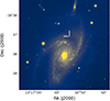 |
Fig. 1. 300s Sloan-r band image obtained with the 1.82 m Ekar Telescope on 2018 April 19. The location of the SN in the host galaxy NGC 5054 is marked. |
Basic information of SN 2018is.
The paper is organised as follows: Section 2 describes the instrumental setups and the tools employed for reducing the photometric and spectroscopic data of SN 2018is. In Section 3, estimation of the explosion epoch of SN 2018is, distance to the SN, and reddening of the host galaxy are reported. Section 4 presents the light curve evolution, and the spectral features are discussed in Section 5. The photometric and spectroscopic parameters of SN 2018is are compared with other SNe II in Section 6. In Section 7, the modelling of the bolometric light curve using both semi-analytical and hydrodynamical methods are discussed. Finally, the nature of the progenitor is discussed in Section 8 and an overall summary of this work is presented in Section 9.
2. Observations and data reduction
The observing campaign of SN 2018is commenced a few hours after its DLT40 discovery, using instruments equipped with broadband UBVgriz filters. PROMPT5 unfiltered DLT40 images are reduced as described in Tartaglia et al. (2018), using the dedicated pipeline and calibrated to the r band. Observations in the UBVgri bands were conducted through the Global Supernova Project (GSP) using the 0.4 m, 1 m, and 2 m telescopes of the Las Cumbres Observatory (LCO). Pre-processing of the images, including bias correction and flat-fielding, is conducted using the BANZAI pipeline (McCully et al. 2018). Subsequent data reduction is performed with lcogtsnpipe (Valenti et al. 2016), a PyRAF-based photometric reduction pipeline. Since the SN was offset from the host galaxy in a region with a smooth background, image subtraction is not required. The UBV band data are calibrated to Vega magnitudes (Stetson 2000), using standard fields observed on the same night by the same telescope. The gri band data are calibrated to AB magnitudes using Henden et al. (2009). Additional optical photometry in BVgriz filters was obtained with (i) the optical imaging component of the Infrared-Optical imager: Optical (IO:O, Barnsley et al. 2016), mounted on the 2 m Liverpool Telescope (LT, Steele et al. 2004), (ii) the Alhambra Faint Object Spectrograph and Camera (ALFOSC) and Stand-by camera (STANcam) on the 2.56 m Nordic Optical Telescope (NOT, Djupvik & Andersen 2010), and (iii) the Asiago Faint Object Spectrograph and Camera (AFOSC) on the 1.82 m Copernico Telescope. The data from these telescopes are reduced similarly, and PSF photometry is performed using DAOPHOT II (Stetson 1987) to compute the instrumental magnitudes of the SN. We also include the ATLAS forced photometry data (Tonry et al. 2018; Smith et al. 2020) in our work.
SN 2018is was also observed with the Ultra-Violet/Optical Telescope (UVOT; Roming et al. 2005) on board the Neil Gehrels Swift Observatory (Gehrels et al. 2004). The observations were carried out in three UV (uvw2: λc = 1928 Å, uvm2: λc = 2246 Å, uvw1: λc = 2600 Å) and three optical (u, b, v) filters at four epochs. UV photometric data are obtained from the Swift Optical/Ultraviolet Supernova Archive (SOUSA1; Brown et al. 2014). The reduction procedure is outlined in Brown et al. (2009), which includes the subtraction of the host galaxy count rate. For estimating the magnitudes, revised zero points and time dependent sensitivity are adopted from Breeveld et al. (2011).
Spectroscopic observations of SN 2018is were carried out from 3.4 to 384 days post-discovery, using (i) the Robert Stobie Spectrograph (RSS, Burgh et al. 2003) with the PG300 lines/mm grating on the Southern African Large Telescope (SALT; Buckley et al. 2006), which covers 3400–9000 Å, at a resolution of ∼18 Å with a 1.5″ slit, (ii) the Goodman High Throughput Spectrograph (GHTS-R; Clemens et al. 2004) on the Southern Astrophysical Research Telescope (SOAR), (iii) the ALFOSC on the NOT, (iv) the Double Beam Spectrograph (DBSP; Oke & Gunn 1982) mounted on the 200-inch Hale telescope at Palomar Observatory (P200), (v) the Boller and Chivens (B&C) Spectrograph with the 300 lines/mm grating on the University of Arizona’s Bok 2.3 m telescope located at Kitt Peak Observatory, which are reduced in a standard way with IRAF (Tody 1986, 1993) routines, (vi) the Blue Channel (BC) spectrograph on the 6.5 m MMT, with the 1200 lines/mm grating covering a range of ∼5700–7000 Å, (vii) the Optical System for Imaging and low-Intermediate-Resolution Integrated Spectroscopy (OSIRIS, grating ID R1000B) mounted on the Gran Telescopio Canarias (GTC), and (viii) the Low Resolution Imaging Spectrometer (LRIS; Oke et al. 1995) on the 10 m Keck-I telescope. The LRIS spectrum was taken using a 1″ aperture with the 560 dichroic to split the beam between the 600/4000 grism on the blue side and the 400/8500 grating on the red side. Taken together, the merged spectrum spans ∼3200–10 200 Å. In addition, a near-infrared low resolution spectrum was obtained with FIRE at the Magellan 6.5 m telescope (8000–25 000 Å). The compiled photometry for SN 2018is and log of spectroscopic observations are provided in Tables A.1 to A.5 of the supplementary material, which is available online2.
Standard procedures are followed for the spectroscopic data, which are reduced within IRAF3. The APALL task is employed to extract one-dimensional spectra, which are subsequently calibrated in wavelength and flux using arc lamps and spectrophotometric standard star spectra, respectively. These standards are observed at comparable airmasses either on the same night or on adjacent nights. Night sky emission lines in the spectra are used to validate the accuracy of wavelength calibration, and necessary shifts are applied as required. In order to account for absolute flux calibration, the spectra are scaled with respect to the photometric data and further corrected for the redshift of the host galaxy.
3. Parameters of SN 2018is
3.1. Explosion epoch and distance
The last non-detection date of SN 2018is is recovered from the ATLAS forced photometry light curve and determined to be 2018 January 12.6 (JD 2458131.1), with a limiting magnitude of 19.85 in the ATLAS o-filter. The SN was first detected in the ATLAS o-filter at a magnitude of 18.01 ± 0.06 on 2018 January 17.7 (JD 2458136.2), 2.6 days before the DLT40 detection on 2018-01-20.3 UT (JD 2458138.8). Therefore, using the last non-detection and first detection from ATLAS, the explosion date is estimated to be 2458133.6 ± 2.6. An alternate method for estimating the explosion epoch is by cross-correlating the SN spectra with a library of spectral templates using the SuperNova IDentification package (SNID, Blondin & Tonry 2007) as done in Gutiérrez et al. (2017). We perform spectral matching on the first two spectra of SN 2018is, obtained on 2018 January 21.0 and 21.3 (0.5 and 0.7 day after discovery, respectively). The best match is determined based on the SNID ‘rlap’ parameter, which quantifies the quality of fit, with a higher value indicating a better correlation. In addition to the ‘rlap’ parameter, the top three spectral matches provided by SNID are checked visually. We found a good match between the spectra of SN 2018is and SN 2006bc (available in the SN IIP templates in SNID from Gutiérrez et al. 2017). SN 2006bc is a LLSN II, with absolute plateau magnitude of −15.1 mag in V band and with a ±4 day uncertainty in the explosion epoch obtained from a photometric non-detection (Anderson et al. 2014). For both spectra of SN 2018is, the best match is found to be with the 9 (± 4) day spectrum of SN 2006bc, with a higher ‘rlap’ value for the second spectrum of SN 2018is. Considering the age of the supernova on 2018 January 21.3 to be 9 (± 4) days post-explosion, the explosion epoch is estimated to be 2018 January 12.3 (± 4), corresponding to JD 2458130.8.
A number of redshift-independent distance estimates are available in the NASA Extragalactic Database (NED) for NGC 5054, the host galaxy of SN 2018is. These estimates span a range from 12.40 Mpc to 27.30 Mpc. The Virgo infall distance to the galaxy NGC 5054 is 25.7 ± 0.2 Mpc, based on the recessional velocity of the galaxy, vVir = 1734 ± 2 km s−1, from HyperLeda (Makarov et al. 2014). The distance estimate of NGC 5054 in the Cosmicflows-3 catalog (Tully et al. 2016) is 18.2 ± 2.5 Mpc.
To obtain an independent distance estimate, we apply the expanding photosphere method (EPM) utilising the early photometric and spectroscopic data of SN 2018is. The EPM is a variant of the Baade-Wesselink method to estimate SN distances (Kirshner & Kwan 1974). We follow the steps and techniques outlined in Dastidar et al. (2018) to implement EPM in SN 2018is. During the early phases, the SN ejecta is fully ionised, and electron scattering is the primary source of opacity at the photosphere. In this phase, the SN can be approximated as radiating like a diluted blackbody. The EPM compares the linear and angular radius of the homologously expanding optically thick SN ejecta to compute the SN distance. The angular radius of the expanding ejecta at any time t can be approximated as
 (1)
(1)
where Bλ is the Planck function at colour temperature Tc, fλ is the flux density received at Earth, Aλ is the extinction at wavelength λ, and ζλ(Tc) is the colour temperature dependent ‘dilution factor’. Here, R = vph(t − t0), where (t − t0) is the time since explosion and vph is the photospheric velocity at the corresponding epoch. Eq. (1) can be written in terms of magnitudes obtained from broadband photometry integrated over the filter response function. The convolution of the filter response function was computed by Hamuy et al. (2001). The dilution factors ζ can be expressed as a function of Tc, as described in Dessart & Hillier (2005). We convert the Sloan r and i magnitudes to I magnitudes by using the equations given by Lupton et al. (2005). The extinction at the central wavelengths of the BVI bands are determined using the high reddening value, AV = 1.34 mag (see Sect. 3.2).
Employing coefficients from Dessart & Hillier (2005), we estimate θ in three filter combinations, {BV}, {BVI}, and {VI}, and list the values in Table 2. The photospheric velocity vph is determined using the Hβ line up to 4.6 days after discovery and the Sc IIλ6246 line up to 45.0 days after discovery. We interpolated the velocity to the photometry epochs using Automated Loess Regression (ALR, Rodríguez et al. 2019).
Derived parameters of SN 2018is for the EPM distance estimate: the angular size (θ), photospheric temperature (T), and the interpolated photospheric velocity (vph).
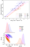 |
Fig. 2. Linear fit to t vs θ/vph to determine the explosion epoch and distance. Top panel shows the fit for the three filter combinations {BV}, {BVI} and {VI}. Bottom panel shows the one and two dimensional projections of the posterior probability distributions of D and t0 for the three filter sets in the corner plot. |
A linear fit is performed on t vs θ/vph to derive the distance, following the equation:
 (2)
(2)
where the slope of the linear equation gives the distance, and the y-intercept provides the time of explosion t0. We used emcee (Foreman-Mackey et al. 2013) to perform the linear fit, and the best fit to the {BV}, {BVI} and {VI} filter sets, along with their 1σ confidence intervals, are shown in the upper panel of Figure 2. The bottom panel of this figure shows the joint likelihoods of the parameters t0 and D for the three filter sets along with the marginalised likelihood functions. The distances are estimated as the mean and standard deviation of the marginalised functions, which are 21.8 ± 1.9 Mpc, 21.3 ± 1.7 Mpc and 24.5 ± 2.2 Mpc for {BV}, {BVI}, and {VI} filter sets, respectively. The corresponding intercept values are −6.2 ± 1.8, −2.8 ± 1.1, and −1.9 ± 1.0 days with respect to the discovery date from ATLAS. We will use the distance and t0 obtained from the {BVI} filter set in the rest of the paper. Thus, the estimated explosion epoch from EPM is JD 2458133.4 ± 1.1 (2018 January 14.9). This value is consistent with those estimated from last non-detection and SNID within the errors, and we will use the EPM estimated explosion epoch throughout this work. The EPM estimated distance (21.3 ± 1.7 Mpc) is small compared to the Virgo infall distance; however it is in agreement with the Cosmicflows-3 distance within the errors. We will use the EPM derived distance in the rest of this paper.
3.2. Extinction
The extinction along the line of sight to the SN due to dust in both the Milky Way (MW) and the host galaxy plays a crucial role in studying the intrinsic nature of the event. Based on the infrared dust maps provided by Schlafly & Finkbeiner (2011), the Galactic reddening for SN 2018is is E(B − V)MW = 0.0708 ± 0.0003 mag.
The empirical relations correlating the NaID (λλ 5890, 5896) equivalent width with the colour excess (e.g. Munari & Zwitter 1997; Poznanski et al. 2012) have been used for various SNe (e.g. Nakaoka et al. 2018; Meza-Retamal et al. 2024). The rest-frame SALT spectrum of SN 2018is, obtained 3.9 days post-explosion, shows a conspicuous feature around 5893 Å (as shown in Fig. 3). The equivalent width of this feature is estimated to be 1.26 ± 0.01 Å. Using Equation (9) from Poznanski et al. (2012), we estimate E(B − V)host to be 0.42 ± 0.08 mag. Given that Poznanski et al. (2012) used the dust maps from Schlegel et al. (1998), we further multiply E(B − V)host by the re-normalisation factor of 0.86, as suggested by Schlafly & Finkbeiner (2011), resulting in E(B − V)host = 0.36 ± 0.07 mag. We note that the accuracy of using the NaID line in low-resolution spectra has been challenged (Poznanski et al. 2011; Phillips et al. 2013), hence the E(B − V)host estimated using this method can only be considered as an upper limit.
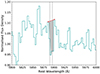 |
Fig. 3. Cut-out of the SALT spectrum showing the blended NaID lines (shaded in the plot). The continuum considered for the estimation of the equivalent width is marked with a red dashed line. |
The V band magnitudes at 50 days, considering only Milky Way (MW) extinction as well as MW plus host extinction, are −13.94 and −15.08 mag, respectively. Furthermore, using SNID, the early spectra of SN 2018is are found to closely match those of the LLSN 2006bc. This, along with the low expansion velocities discussed in Sect. 6.2, suggests that SN 2018is belongs to the LLSNe II category. Therefore, as an independent estimate of the host galaxy extinction, we compare the MW-corrected colour evolution of SN 2018is with that of the well-observed LLSN II, SN 2005cs, and calculate the shift required for SN 2018is’s colour to align with that of SN 2005cs. The E(B − V)host estimated using this method is 0.12 ± 0.06 mag, which is three times lower than the value obtained from the NaID feature. The resulting colour curve, using both estimates, is shown in Fig. 5.
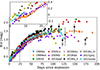 |
Fig. 5. (B − V) colour evolution of SN 2018is, corrected for the high (AV = 1.34 mag) and low (AV = 0.59 mag) extinction scenarios, are compared with other SNe II. |
Given the caveats associated with different methods for calculating host-galaxy extinction, and with no method being definitively preferable, we are considering two values of extinction in this study. Therefore, we adopt a total E(B − V)tot of 0.19 ± 0.06 as the low-extinction estimate and 0.43 ± 0.07 mag as the high-extinction estimate, with the corresponding AV values being – AV, lr = 0.59 ± 0.19 mag and AV, hr = 1.34 ± 0.21 mag, assuming total-to-selective extinction ratio, RV = 3.1, and using the extinction function from Gordon (2024) (also see Gordon et al. 2009, 2021, 2023; Fitzpatrick et al. 2019; Decleir et al. 2022).
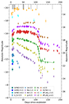 |
Fig. 4. Absolute (corrected for AV = 1.34 mag) and apparent magnitude UV and optical light curves of SN 2018is, shifted arbitrarily for clarity. Vertical grey lines mark the epochs of spectroscopic observations. Parameterized fit to the V band light curve Valenti et al. (2016) is also shown. |
4. Light curve evolution
The multiband optical and UV absolute and apparent magnitude light curves of SN 2018is are shown in Fig. 4. The high reddening value, which is converted to extinction estimates in the different bands using the dust-extinction law from Gordon et al. (2023), are used to derive the absolute magnitudes. Initially, the light curves exhibit an increase in brightness for the first 10 days following the assumed explosion epoch, followed by a decrease in the bluer filters. Meanwhile, in the r and i bands, the luminosity increases until 28 days and remains nearly constant thereafter. The plateau phase, lasting nearly 100 days, is relatively short for typical LLSNe II (Pastorello et al. 2009; Spiro et al. 2014). The V band light curve shows a linear decline with a slope of 1.04 ± 0.03 mag (100 d)−1, which is steeper than usual for LLSNe II (Pastorello et al. 2009; Spiro et al. 2014). Post-maximum decline rates in the r and i bands are 0.26 ± 0.02 mag (100 d)−1 and 0.02 ± 0.02 mag (100 d)−1, respectively, consistent with other LLSNe II (Pastorello et al. 2009; Spiro et al. 2014). The decline rates in the plateau and the tail phase in the BgVri bands are provided in Table 3.
Light curve slopes at different phases.
Using Equation (1) from Valenti et al. (2016), which is the same as Equation (4) from Olivares et al. (2010) without the Gaussian component, we fit the V band light curve to derive parameters that can be compared to those of other LLSNe II. From the best fit, over-plotted on the V band light curve in Figure 4, we determine tPT, the time from explosion to the transition point between the end of the plateau and the start of the radioactive tail phase, to be 113.9 ± 1.1 d. The parameter w0 gives an estimate of the duration of the post-plateau decline until the onset of the radioactive tail phase to be (6 × w0) 15 days. The parameter a0 = 2.4 ± 0.1 mag, which quantifies the magnitude drop when the light curve transitions from the photospheric phase to the radioactive tail, is typical for SNe IIP (Olivares et al. 2010), although, under-luminous objects generally show a larger drop of about 3–5 mag (Spiro et al. 2014; Valenti et al. 2016).
The decay rates in the tail phase of the bolometric light curve of LLSNe II are generally smaller than the 0.98 mag (100 d)−1 expected from the 56Co to 56Fe decay assuming complete γ-ray trapping (Pastorello et al. 2009; Spiro et al. 2014). For SN 2018is, the decline rates in the tail phase for the B, g, V, r and i band light curves are 0.3 ± 0.4, 0.4 ± 0.2, 0.7 ± 0.2, 0.8 ± 0.1 and 0.6 ± 0.1 mag (100 d)−1, respectively. The light curves of SN 2005cs exhibit similar decline rates between 140–320 day in the BVRI bands, measured at 0.32, 0.46, 0.71, and 0.77 mag (100 d)−1, respectively. (Spiro et al. 2014) calculated the decline rate of SN 2003Z in the tail phase (> 150 d) in VRI bands to be 0.67, 1.05, and 0.58 mag (100 d)−1, respectively. It has been proposed that the shallower slope in LLSNe II is due to an additional radiation source generated in the warm inner ejecta (Utrobin 2007).
In order to compare the light curve and spectral properties of SN 2018is with other Type II SNe, we construct a comparison sample constituting the normal luminosity Type II SN 1999em, and a number of intermediate and LLSNe II. The distances, reddening and references of the comparison sample and some of the physical parameters estimated in this work from their light curves are provided in Tables A.6 and A.7 of the online supplementary material4.
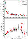 |
Fig. 6. Temperature and radius evolution of SN 2018is, obtained by fitting a blackbody to the SED constructed from the observed photometric fluxes. Estimates are shown for both low-reddening (LR) and high-reddening (HR) corrected fluxes, as well as for SN 2005cs for comparison. |
4.1. Colour and temperature evolution
The extinction-corrected colour evolution of SN 2018is is compared to a subset of SNe II from the comparison sample in Fig. 5. In the low-extinction case, SN 2018is exhibits a colour that falls on the red end of the sample. If only the MW extinction correction is applied, the colour of SN 2018is would be 0.12 mag redder than the colour obtained using the low-extinction estimate. Studies by Pastorello et al. (2009) and Spiro et al. (2014) have noted that LLSNe II, when compared to normal SNe II, tend to have redder intrinsic colours.
In SN 2018is, a rapid increase in the B − V colour by around 0.2 mag is observed in the first 5 days, as shown in the zoom-in plot. This is followed by a slight decrease and then a rapid rise after 10 days. Similar behaviour is noted in the colour evolution of SNe 2018lab and 2022acko (Pearson et al. 2023; Bostroem et al. 2023). SNe 2018lab, 2021gmj and 2022acko exhibit a trend towards bluer colours after the end of the recombination phase, around 100 and 110 days, respectively, unlike SNe 2003Z and 2005cs, which evolves towards redder colours. However, due to the large error bars associated with the colour of SN 2018is after the recombination phase, it is difficult to ascertain whether it followed a pattern similar to SN 2005cs or SN 2022acko. When using the high reddening estimate, SN 2018is is about 0.24 mag bluer than with the low reddening estimate, aligning more closely with the colour evolution of SNe 2016aqf, 1999em, and 2009ib (Müller-Bravo et al. 2020; Takáts et al. 2015).
As the SN expands and cools, the photospheric temperature and radius evolve over time. These parameters can be traced by fitting a blackbody model to the spectral energy distribution (SED) at different epochs. The SED is constructed using SuperBol (Nicholl 2018), as described in Sect. 7. The top and bottom panels of Figure 6 illustrate the temperature and the radius evolution of SN 2018is for both high and low reddening scenarios, compared to that of SN 2005cs. In the high reddening scenario, the temperatures during the first 60 days are higher than those of SN 2005cs. However, the temperature evolution in the low reddening scenario aligns more closely with SN 2005cs. Overall, SN 2018is shows a gradual temperature decline during the first 30 days, followed by a slower decline from around 6000 K to 4000 K over the next 100 days. The radius increases rapidly in the first 30 days and then continues to expand slowly, similar to the evolution observed in SN 2005cs. Around day 110, a rapid decline in radius is observed in SN 2018is, whereas SN 2005cs exhibits an increase in radius before declining, although we note that the error bars are large at these times.
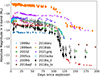 |
Fig. 7. Comparison of absolute V band light curves of SN 2018is with other SNe II. The magnitudes are corrected for distance and reddening. |
4.2. Absolute magnitude comparison and 56Ni mass
In Figure 7, the absolute V band magnitude of SN 2018is is compared to a subset of SNe II from the comparison sample. Typically, LLSNe II exhibit long plateaus (> 100 days), although also some normal luminosity SNe II (e.g. SN 2015ba, Dastidar et al. 2018) have extended plateaus. In H-rich SNe II, the plateau length is primarily influenced by the H envelope mass and the ejecta velocity, with a modest contribution from the energy released by 56Ni decay (Kasen & Woosley 2009; Morozova et al. 2018; Kozyreva et al. 2019; Martinez et al. 2022). The low ejecta velocity in LLSNe II, which is typically a factor of a few lower than in normal luminosity Type II SNe, results in higher ejecta densities. This slows the recombination wave, thereby extending the plateau duration. In normal luminosity Type II SNe, while higher 56Ni yields can extend the plateau length by 10–20% (Kasen & Woosley 2009), the higher expansion velocity leads to lower densities and a faster-moving recombination wave, resulting in an overall shorter plateau.
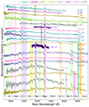 |
Fig. 8. Spectral evolution of SN 2018is from 6.2 to 106.1 day is shown and the prominent features are marked. |
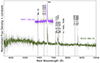 |
Fig. 9. Nebular phase spectra at 168.2 and 386.7 day of SN 2018is are shown and the prominent features are marked. |
LLSNe II events like SNe 2003Z and 2005cs exhibit longer plateaus compared to SN 2018is, with similar plateau luminosities, when the low reddening scenario is considered. In the high reddening scenario, the plateau luminosity of SN 2018is is a closer match to SNe 2018lab and 2022acko. The fall from the plateau in the case of SN 2018is is adequately sampled and has a similar plateau length as SN 2018lab. Moreover, from this figure, it is apparent that SNe II with similar plateau luminosities can have a range of tail-luminosities (−9.5 to −12.5), depending on the amount of 56Ni produced in the explosion.
For SN 2018is, we estimate the synthesised 56Ni mass from the tail bolometric luminosity, which is obtained from the tail V band magnitudes using a bolometric correction (BC) from Hamuy (2003). The tail V band magnitudes at two epochs, 148.6 and 173.6 d, are considered, and the corresponding mean bolometric luminosities are 8.3 ± 1.4 × 1039 erg s−1 and 1.6 ± 0.3 × 1040 erg s−1 for the low and high reddening scenarios, respectively. This results in a mean 56Ni mass of 0.0026 ± 0.0004 M⊙ and 0.0051 ± 0.0009 M⊙, for the low and high reddening scenarios, respectively. In addition, using BCs in the Vri bands from Rodríguez et al. (2021), determined using a larger sample of SNe II, the 56Ni masses are 0.0027 ± 0.0009, 0.0030 ± 0.0008, 0.0030 ± 0.0007 M⊙, respectively, for the low reddening scenario and 0.0052 ± 0.0017, 0.0053 ± 0.0015, 0.0046 ± 0.0011 M⊙, respectively, for the high reddening scenario, closely matching the earlier value. The weighted average of 56Ni mass using BCs from Rodríguez et al. (2021) are 0.0029 ± 0.0004 and 0.0049 ± 0.0008 M⊙. Both values align well with those of other LLSNe II.
5. Key spectral features
5.1. Features in the optical spectra
The first spectrum of SN 2018is was obtained 6.2 days post-explosion. The spectral evolution from 6.2–106.1 days of SN 2018is is shown in Figure 8. Until 7.4 d, the spectra of SN 2018is show a blue continuum with weak and shallow P Cygni profiles of the Balmer H lines. A weak He Iλ5876 feature is visible until 7.4 days, after which it disappears. The Fe IIλ5018 line emerges as early as 9.5 days. An absorption feature at λ6300, which we identify as Si IIλ6355, is discernible between 11.6 and 30.3 days, disappearing afterwards. This feature was also detected in the early spectra of SN 2005cs (Pastorello et al. 2006). We attribute this feature to Si II, given its velocity similarity with other metal lines (around 3000 km s−1 at 11.6 days and 1300 km s−1 at 30.3 days).
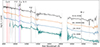 |
Fig. 10. NIR spectrum of SN 2018is obtained at 16.3 day is compared to intermediate luminosity Type II SNe 2009N, 2012A as well as a LLSN ASASSN-14jb. |
Two nebular phase spectra of SN 2018is, at 168.2 and 386.7 days, are shown in Figure 9. In the 386.7 day spectrum, besides prominent Hα emission, the strongest feature is the λ7300 doublet emission, associated with [Ca II] lines λλ7291,7324. An unblended emission bluewards of [Ca II] lines is identified as [Fe II] λ7155, observed in the late time spectra of several SNe II (e.g. 2016aqf, 2016bkv). The [O I] λλ6300, 6364 doublet can be identified in this spectrum, while the Ca II NIR triplet is inconspicuous. A weak [Ni II] λ7378, produced by stable 58Ni, a nuclear burning ash, is identifiable. The presence of [Ni II] is a unique signature of neutron excess in the innermost Fe-rich layer, and hence it is a crucial tracer of explosive burning conditions (Wanajo et al. 2009). This feature has been analysed and discussed in more detail in Sect. 8.1.
5.2. Features in the NIR spectrum
The 16.3 day NIR spectrum of SN 2018is is shown in Fig. 10, alongside those of SN 2009N (Takáts et al. 2014) and two other Type II SNe from Davis et al. (2019) for comparison. The spectrum of SN 2018is displays the Ca II NIR triplet, partial blends of Pγ λ10940 and Sr IIλ10915 and Pβ λ12820, and Brγ λ21650. The location of Pα λ18750 is contaminated by strong telluric absorption, making it indiscernible.
In normal luminosity Type II SNe, such as SN 2012A (Tomasella et al. 2013), Pγ and He Iλ10830 lines are strongly blended which gives rise to a broad absorption feature. However, LLSNe II, with their narrow features, exhibit partially unblended Pγ, Sr II, and He I lines, as seen in the spectra of SNe 2009N and 2018is. C Iλ10691 also contributes to the broad absorption that is clearly absent in SN 2018is. In normal Type II SNe with a relatively high 56Ni yield, the absorption in this region is primarily dominated by He I, which is produced via non-thermal excitation when 56Ni is located close to the He region in the ejecta (Graham 1988). However, in LLSNe II, where the 56Ni yield is minimal, He I is not expected to significantly contribute to this feature. Instead, Pγ, Sr II and C I dominate the absorption (Pastorello et al. 2009).
The Pβ line, visible in all the SNe, exhibits a symmetric P Cygni profile, which is dominated by its emission feature with very little absorption in SNe 2012A, ASASSN-14jb, while in SN 2018is a narrow absorption component is visible. The Brackett series hydrogen line, Brγ is prominent in absorption in both SNe 2009N and 2018is. Overall, in the NIR spectra, the emission features of the comparison SNe are broad at early times, even in the case of ASASSN-14jb, which is a LLSN (MVpeak = −14.93 mag). In contrast, the features of SN 2018is are remarkably narrower, which is also evident in the optical spectra comparison discussed in Sect. 6.2.
 |
Fig. 11. Position of SN 2018is on the absolute magnitude at 50 day (based on the low reddening (LR) and high reddening (HR) scenarios) vs. tPT, V band slope (s2) and 56Ni mass plot are shown alongside other SNe II. The sample from Anderson et al. (2014) and Valenti et al. (2016) are marked with a ‘+’, from Dastidar et al. (2024) with an ‘x’, and from this work with a ‘⋆’. |
6. Juxtaposition with other type II SNe
6.1. Comparison based on photometric parameters
We compare some of the photometric parameters of SN 2018is with those of a sample of SNe II from the literature (Anderson et al. 2014; Valenti et al. 2016; Dastidar et al. 2024). In Fig. 11, the absolute magnitude at 50 day (MV50 d) is plotted against tPT, slope during the plateau phase (s2), and log(MNi). A general trend is observed where higher luminosity SNe II tend to have a shorter and steeper plateau, as well as a larger 56Ni mass yield, consistent with findings from earlier studies (e.g. Anderson et al. 2014; Valenti et al. 2016). While the absolute magnitude in the high-reddening scenario for SN 2018is fits this trend, in the low-reddening scenario, SN 2018is appears slightly offset from the general trend in the MV50d vs. tPT and s2 plots.
In Figure 12, we have plotted tPT vs s2 for the SNe II sample from the literature alongside SN 2018is. These parameters are known to exhibit a negative correlation, where SNe II with longer plateaus tend to have shallower decline rates. The figure is colour-coded by the V band absolute magnitude at 50 day. SNe for which MV50 d is not available are shown in grey. While SN 2018is follows the overall trend, its decline rate is higher than that of other LLSNe II. It also has a shorter tPT similar to SNe 2018lab and 2022acko5.
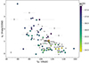 |
Fig. 12. Position of SN 2018is on the V band slope (s2) vs. tPT plot, alongside other SNe II. The points are colour-coded with MV50 d values. SNe for which MV50 d is not available are shown in grey. SN 2018is is colour-coded with MV50 d based on the high reddening scenario. |
6.2. Comparison based on spectroscopic features
Figure 13 shows the comparison of the early spectra of SN 2018is with similar epoch spectra of other LLSNe II. All the spectra exhibit a blue continuum with superimposed P Cygni profiles of H Balmer lines, featuring weak absorption components. The emission components of the H Balmer lines in SN 2018is are narrower than those in the spectra of the comparison sample, indicating a lower expansion velocity of the ejecta compared to the others.
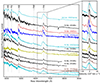 |
Fig. 13. Early spectra of SN 2018is are compared to spectra of other LLSNe II at similar epochs. The right panel shows the Hα region in velocity space, with the shaded area representing twice the FWHM of the Hα line for SN 2018is. |
The velocities of various elements in the ejecta, such as Hα, Hβ, Fe IIλ5169, and Sc IIλ6246 lines, are estimated from the position of their absorption minima and are compared to a subset of SNe from the comparison sample as shown in Figure 14. Before 30 days, the H Balmer line velocities of SN 2018is are the lowest among the comparison SNe. After 30 days, the H Balmer line velocities settle at around 3000 km s−1 with little evolution thereafter. In contrast, the velocities of the H Balmer lines in SNe 1999br, 2003Z and 2005cs, which are higher in the early phases, drop below those of SN 2018is at later phases.
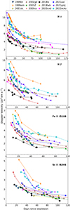 |
Fig. 14. Velocity evolution of the H Balmer and metal lines are compared with a sample of low and standard luminosity SNe IIP. |
Meanwhile, SNe 2002gd, 2020cxd (Valerin et al. 2022), 2021gmj and 2022acko also exhibit a flattening in velocity evolution after an initial rapid decline, similar to SN 2018is. This flattening could occur if the inner layers of the SN ejecta are relatively H-poor, causing the H Balmer absorption to originate from the H-rich outer (and therefore higher-velocity) ejecta layers even during the later phases (Faran et al. 2014). This scenario is typical when the pre-SN star has a low H-envelope mass, as proposed for fast-declining SNe II. However, in the case of LLSNe II, the formation of Ba IIλ6497 is the probable cause for the flattening, which complicates the estimation of the true absorption minimum of Hα. Compared to the sample of LLSNe II, the expansion velocity of Fe IIλ5169 in SN 2018is is consistently lower at all epochs. Similarly, the Sc IIλ6246 velocities are on the lower end of the comparison sample. The photospheric velocity, inferred from the Sc IIλ6246 minimum, rapidly decreases from ∼2500 km s−1 at about two weeks to less than 800 km s−1 at ∼100 days.
Cut-outs of the main features in the nebular phase spectrum of SN 2018is, along with a subset of the comparison sample, are shown in Figure 15. Most of the features in the nebular spectrum of SN 2018is are weaker compared to other LLSNe II. [O I] λλ6300, 6364, and Hα are similar in strength to those in SN 2005cs, while SNe 1997D and 2018lab exhibit much stronger features. However, features such as [Fe I], [C I] and Ca II NIR triplet, which are present in the spectrum of SN 2005cs, are not discernible in the spectrum of SN 2018is, which could be due to low signal-to-noise ratio in the NIR.
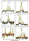 |
Fig. 15. Comparison of the nebular spectra of SN 2018is with other LLSNe II at similar epochs. The panels show the key spectral features [O I] λλ6300, 6364, Hα, [Fe II], [Ca II], [Ni II], [Fe I], and Ca II lines. |
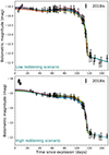 |
Fig. 16. Bolometric magnitude evolution of SN 2018is considering both the low extinction and high extinction estimates are shown in the top and bottom panels, respectively, and the corresponding 50 best-fitted light curves are over-plotted. |
7. Bolometric light curve modelling
7.1. Semi-analytical modelling
In order to derive estimates of the explosion and progenitor parameters from the bolometric light curve, we employed the semi-analytical modelling of Nagy et al. (2014). The bolometric light curve of SN 2018is is constructed using SuperBol (Nicholl 2018), by using uvw1 and UBgVri magnitudes up to 9.4 days, followed by UBgVri magnitudes up to 34.8 days and thereafter BgVri magnitudes. This is done to ensure that the UV contribution is taken care of in the early part of the light curve. The de-reddened magnitudes supplied to the routine are interpolated to a common set of epochs and converted to fluxes. The fluxes are used to construct the SED at all the epochs. The routine then fits a blackbody function to the SED, extrapolating to the UV and IR regimes to estimate the true bolometric luminosity.
We use the Markov Chain Monte Carlo (MCMC) version of the semi-analytic light curve code of Nagy et al. (2014), developed in Jäger et al. (2020), for fitting the output model to the observed light curves. The semi-analytic code of Nagy et al. (2014) is based on the original model of Arnett & Fu (1989). The model assumes a homologously expanding, spherically symmetric SN ejecta and uses the diffusion approximation for the radiation transport. However, the simple diffusion-recombination model that assumes constant opacity in the ejecta limits the accuracy of the derived physical parameters. For example, the constant opacity approximation results in a negative correlation between Thomson opacity (κ) and ejecta mass (Mej), which has a significant effect on the estimated Mej. The correlation between the various explosion parameters makes it important to explore the parameter space with the MCMC approach. Jäger et al. (2020) applied this approach to obtain the best estimates and uncertainties for the core parameters.
In our case, the parameters are the initial radius (R0), the ejected mass (Mej), and the energies (total explosion energy: E0 = Ekin + Eth, kinetic: Ekin, thermal: Eth), ejecta velocity (vexp) and 56Ni mass. We searched for the best-fit parameters in the parameter space: R0: (2–10) × 1013 cm, Mej: 4–20 M⊙, Ekin: 0.1–2 foe (1 foe = 1051 erg), Eth: 0.001–1 foe, κ: 0.05–0.4 cm2 g−1. The recombination temperature is fixed to 5500 K. The initial expansion velocity is set to 2500 km s−1 with an uncertainty of 250 km s−1, which is basically the velocity obtained from the minima of the Sc IIλ6246 absorption profile at 18 day as the starting day of the fitting is set to 20 day after the explosion. The parameter estimates obtained from the MCMC routine for both the low and high reddening scenarios are listed in Table 4.
Best-fit core parameters for the true bolometric light curve of SN 2018is using Nagy et al. (2014) and Jäger et al. (2020) for the low reddening (LR) and high reddening (HR) scenarios.
The reported parameter values are the mean of the joint posterior, corresponding to the best-fitting solution. The uncertainty limits are derived from taking the 95th percentile of the marginalised posterior probability density function and subtracting the 50th percentile for the upper error. The lower error is estimated by subtracting the 5th percentile from the 50th percentile. The top and bottom panel of Figure 16 shows the observed bolometric magnitude evolution of SN 2018is corrected for low and high extinction estimate, respectively, and the corresponding best fifty model light curves from the 3 × 10⁵ iterations in the MCMC, while the posterior distribution of the parameters and their correlations are shown in Figures A.1 and A.2 of the online supplementary material6. The parameter estimates and their uncertainties are also provided in Table 4. There are known parameter correlations (Arnett & Fu 1989; Nagy et al. 2014) between R0 and Eth, ejected mass and opacity; kinetic energy and opacity, which can also be seen in the corner plot. Since the parameter pairs: Eth–R0 are significantly correlated, separate determination of the quantities in the pair is not possible. Rather, the product of the pair should be used as an independent parameter. Assuming a remnant neutron star mass of 1.5–2 M⊙, the lower limit of the progenitor mass would be ∼8–10 M⊙, which indicates that SN 2018is is most likely arising from the collapse of a progenitor close to the lower mass limit for core collapse.
Pre-supernova structure summary and CSM parameters from SNEC models.
7.2. 1D hydrodynamical modelling
We use the open-source 1D radiation hydrodynamics code, Supernova Explosion Code (SNEC, Morozova et al. 2015), for multi-band light curve modelling to infer the progenitor parameters and explosion properties of SN 2018is. SNEC is a local thermodynamic equilibrium (LTE) code that employs grey opacities without spectral calculations. The code takes progenitor model, explosion energy, 56Ni mass, and 56Ni mixing as inputs and simulates a range of outputs, including multi-band and bolometric light curves, photospheric velocity, and temperature evolution.
For the progenitor, we adopt a set of non-rotating solar metallicity RSG models from Sukhbold et al. (2016), which are computed using the stellar evolution code KEPLER (Weaver et al. 1978). The lowest mass limit of progenitor models for Fe core collapse, as generated in Sukhbold et al. (2016), is 9 M⊙. The length of the plateau phase in the simulated light curves is observed to increase with higher ZAMS mass, whereas it decreased with an increase in explosion energy. We generate a grid of SNEC models encompassing ZAMS masses between 9 and 11 M⊙ in steps of 0.5 M⊙, explosion energy within 0.1–0.5 foe in steps of 0.01 foe, while maintaining a constant 56Ni mass of 0.0049 M⊙. The 56Ni mixing parameter, representing the mass-coordinate until which 56Ni is mixed outwards, is fixed to 2 M⊙.
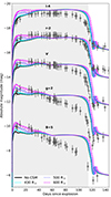 |
Fig. 17. Multi-band model light curves for scenarios with ‘No CSM’ and CSM extents of 430, 500 and 600 R⊙, with KCSM values of 2, 3, 4, and 5 × 10¹⁸ g cm−1, are shown alongside the observed light curves. The shaded region marks the area below tPT, after which non-LTE conditions dominate, making SNEC models invalid. |
The best-fitting progenitor model is determined by finding the minimal χ2, computed as
 (3)
(3)
where mλobs(t) and Δmλobs(t) are the magnitudes and their corresponding errors at time t, mλmodel(t) are the model magnitudes at time t, λ denotes the Vri filters, N is the number of filters, Nλ is the total number of observed data points in filter λ, Nvel is the number of observed photospheric velocity data points, and vobs(t) and Δvobs(t) are the observed photospheric velocity and their error at time t. The model photospheric velocity at time t is denoted by vmodel(t). We compute mλcalc by reddening the model magnitudes to compare with the observed magnitudes (without extinction correction). We vary AV between the Galactic extinction value (0.22 mag) and the high extinction value considered in this work (1.34 mag). For the fitting, we also allow the distance to vary between 19.6 Mpc and 23 Mpc based on the mean value and the error in the distance (21.3 ± 1.7 Mpc). We did not include the bluer band light curves, such as the UBg bands, for estimating the minimum chi-square, as these light curves are more susceptible to being affected by line blanketing at later phases. We identify the best-fit solution as corresponding to a 9.0 M⊙ ZAMS star, with a pre-SN mass of 8.75 M⊙, and a pre-SN stellar radius of 403 R⊙, and an explosion energy of 0.19 foe.
To improve the fit to the early light curve (< 30 days), we add a wind-like circumstellar medium (CSM) profile to the best-fit progenitor model, as in Dastidar et al. (2024) and Reguitti et al. (2024). The density profile follows ρ = KCSMr−2, where KCSM is the mass-loading parameter. We generate models with KCSM values from 2 to 5 × 10¹⁸ g cm−1 and CSM extents (RCSM) of 430, 500, and 600 R⊙.
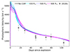 |
Fig. 18. Model photospheric velocities for scenarios with ‘No CSM’ and CSM extents of 430, 500 and 600 R⊙, and KCSM values of 2, 3, 4, 5 × 10¹⁸ g cm−1 are shown, alongside the line velocity of Sc IIλ6246 for SN 2018is. |
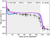 |
Fig. 19. Model bolometric luminosities for scenarios with ‘No CSM’ and CSM extents of 430, 500 and 600 R⊙, and KCSM values of 2, 3, 4, 5 × 10¹⁸ g cm−1 are shown, alongside the observed bolometric luminosity of SN 2018is. The shaded region marks the area below tPT, after which non-LTE conditions dominate, making SNEC models invalid. |
Fig. 17 shows the absolute model magnitudes alongside the observed light curves. The distance and extinction correction (AV) applied to the observed light curves are 23 Mpc and 1.18 mag, respectively. Thus, these models suggest a total E(B − V) value of 0.38 mag, close to the high reddening estimate. Fig. 18 compares model photospheric velocities with the Sc II line velocities, while the model bolometric luminosity alongside the observed bolometric luminosity for SN 2018is is shown in Fig. 19. The early bolometric luminosity is better reproduced with KCSM values of (2–5) × 1018 g cm−1 and RCSM = 600 R⊙, which we will consider as the best-match models. The progenitor, explosion and CSM parameters for the best-match model are tabulated in Table 5. The CSM mass is estimated to be 0.17–0.43 M⊙, using

where R⋆ = 403 R⊙ is the pre-supernova radius.
We note that these models overestimated the plateau length by ∼3 days, while the model photospheric velocity mostly corresponds to the upper limit of the observed Sc II line velocities. The explosion energy, which influences both luminosity and expansion velocity, also plays a crucial role in determining the plateau length, with higher energies generally leading to shorter plateaus. Therefore, the plateau length of SN 2018is could theoretically be modelled with an increased explosion energy, though this would result in velocities exceeding those observed. Kozyreva et al. (2022) showed that plateau length might depend on the viewing angle in asymmetric explosions, offering a possible explanation for the plateau-length discrepancy in SN 2018is. Overall, light curve modelling indicates that SN 2018is is consistent with a low-energy explosion (1050 erg) of a low-mass star (9 M⊙), with the shorter observed plateau potentially due to an asymmetric explosion.
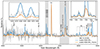 |
Fig. 20. 386.7 day nebular spectrum of SN 2018is compared to the 9 M⊙ model and hydrogen-zone model of Jerkstrand et al. (2018). Narrow emission lines (probably) from the host galaxy in the observed spectrum have been removed. |
8. Discussion
8.1. Nebular constraints on the progenitor mass
8.1.1. Comparison with spectral models
During the nebular phase, the ejecta becomes optically thin, revealing the SN core. Analysing nebular spectra, therefore, provides insight into the core properties, including its mass (Jerkstrand et al. 2012; Dessart et al. 2021). The mass of the stellar core, in turn, serves as an indicator of the star’s initial mass. We constrain the ZAMS mass of the progenitor by comparing the nebular spectra to the nebular spectral models of Jerkstrand et al. (2018). In their study, they observed that the luminosity of the [O I] line is primarily influenced by the progenitor’s ZAMS mass (Jerkstrand et al. 2012). Progenitors with higher masses tend to display more pronounced [O I] features in their nebular spectra.
To allow a consistent comparison, we scale the model spectrum to match the 56Ni mass of 0.0049 M⊙, distance and epoch of the SN 2018is nebular spectrum. Additionally, owing to uncertainties in extinction, all spectra are normalised to their respective Hα peak flux. Figure 20 shows the comparison of the 390 day nebular spectrum of SN 2018is with the scaled nebular spectral models for a 9 M⊙ RSG progenitor. The 9 M⊙ progenitor model of Sukhbold et al. (2016), evolved with KEPLER, is used in Jerkstrand et al. (2018). Additionally, we plot the 9 M⊙ ‘pure hydrogen-zone’ model in Figure 20. In this model, the progenitor is composed entirely of material from the hydrogen envelope. It is anticipated that this model would resemble the nebular spectra of ECSNe, characterised by faint features such as Mg I], Fe I, [O I], He I, [C I] λ8727, and O Iλ7774, along with a prominent O Iλ8446 line. The two insets in Figure 20 zoom in on the [O I] and [Ca II] regions. The [O I] emission of SN 2018is lies between the two models, whereas [Ca II] is better matched by the H-zone model.
Although Fe I lines between 7900–8400 Å and [C I] λ8727, which are present in the 9 M⊙ RSG progenitor model, are absent in SN 2018is, features such as [Fe II], [Ni II], and (weak) He I are discernible. The O Iλ8446 line, which is an important diagnostic in the nebular spectra of ECSNe and is present in the H-zone model, is also absent in the observed spectrum. The presence of He, Fe, and Ni lines in the observed spectrum may imply the presence of He shell in the ejecta. The 9 M⊙ model also predicts strong [O I] λλ6300, 6364 doublet and Mg I], both of which arise from the O zone. In SN 2018is, while the [O I] λλ6300, 6364 doublet is discernible, Mg I] cannot be identified due to the low SNR of the nebular spectrum. From this comparison, it is evident that the progenitor mass of SN 2018is is 9 M⊙ or lower. The possible presence of a He-shell suggests that it likely underwent Fe-core collapse before exploding as a SN.
8.1.2. Constraints from forbidden lines
The nebular spectrum at 386.7 day shows several forbidden transitions, which can aid in constraining the stable Ni to Fe abundance ratio. Theoretical model predicts that the ZAMS mass of the progenitor decreases with increasing Ni/Fe abundance ratio, and hence, this ratio can be used to put constraints on the progenitor mass. The 386.7 days spectrum is calibrated to extrapolated gVri bands photometry. Using Gaussian components, we fit the seven dominant line transitions in the 7100–7500 Å region, which are [Ca II] λλ7291, 7323, [Fe II] λ7155, [Fe II] λ7172, [Fe II] λ7388, [Fe II] λ7453, [Ni II] λ7378, and [Ni II] λ7412. The relative luminosities of lines from a given element are taken from Jerkstrand et al. (2015). So, the iron lines are constrained by L7453 = 0.31 L7155, L7172 = 0.24 L7155, L7388 = 0.19 L7155, and the nickel lines are constrained by L7412 = 0.31 L7378. A single line width for all lines, the full width at half-maximum (FWHM) velocity V, is used. The free parameters are then L7291, 7323, L7155, L7378, and V. As shown in Figure 21, a good fit is obtained for L7291, 7323 = 1.2 × 1037 erg s−1, L7155 = (2.7 ± 0.4) × 1036 erg s−1, L7378 = (1.8 ± 0.3) × 1036 erg s−1, and V = 1400 km s−1. From this we determine a ratio L7378 /L7155 = 0.67. The iron-zone temperature is estimated to lie in the range 2550–2650 K, using the ratio of L7155 and M56Ni (in the high reddening scenario) to be (8.9 ± 1.7) × 1038 erg s−1 M . Using the above temperature, the Ni to Fe abundance ratio is found to be 0.04, which is 0.7 times the solar value (0.056, Lodders 2003). However, as noted by Jerkstrand et al. (2015), primordial Fe and Ni may contaminate the observed ratio, potentially leading to an underestimation by a factor of three. Consequently, the estimated Ni/Fe ratio derived from the 386.7 day spectrum should be regarded as a lower limit and could be as high as 0.12. Theoretical studies indicate that CCSNe originating from moderate-mass progenitors (9–11 M⊙) exhibit higher Ni/Fe abundance ratios (Woosley & Weaver 1995). For example, the models of Woosley & Heger (2007) predict a Ni/Fe ratio of 0.04 for a 15 M⊙ ZAMS mass star. Based on these predictions, the upper limit of the progenitor’s ZAMS mass for SN 2018is can be constrained to 15 M⊙. Finally, it is important to note that recent theoretical models present conflicting perspectives on the dependence of the Ni/Fe abundance ratio on the progenitor’s ZAMS mass. While 1D explosion nucleosynthesis models by Sukhbold et al. (2016) do not show a significant Ni/Fe enhancement for moderate-mass progenitors, 3D models of Fe-core CCSNe (Burrows et al. 2024; Wang & Burrows 2024) suggest that initial velocity perturbations can significantly affect the Ni/Fe ratio, yielding values from sub-solar to as high as 50 times the solar value. Thus, using the Ni/Fe abundance ratio to constrain the progenitor’s ZAMS mass remains highly uncertain.
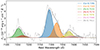 |
Fig. 21. Spectrum cut-out of the 386.7 day spectrum showing the Gaussian fits to determine the [Ni II] λ7378/[Fe II] λ7155 in SN 2018is. |
We estimate the [O I] λλ6300, 6364 luminosity by Gaussian fit to be 2.9 × 1036 erg s−1, assuming a ratio [O I] λ6300/[O I] λ6364 = 3. The luminosity ratio of [Ca II]/[O I] is considered a good diagnostic for the He core mass, and consequently the progenitor mass (Fransson & Chevalier 1987, 1989), with higher ratios corresponding to lower ZAMS masses. For SN 2005cs, this ratio was estimated to be ∼4.2 ± 0.6 (Pastorello et al. 2009). The [Ca II]/[O I] luminosity ratio is 4.1 for SN 2018is, which indicates a low-mass progenitor for SN 2018is. However, the line ratio is only a rough diagnostic of the core mass due to the contribution to the emission from primordial O in the hydrogen zone (Jerkstrand et al. 2012; Maguire et al. 2012) and the effects of mixing, which can complicate the determination of relative abundances based on line strengths, as noted by Fransson & Chevalier (1989).
8.2. Investigating the electron-capture nature of SN 2018is
The progenitor mass of SN 2018is, as estimated from the analysis of nebular spectra and from semi-analytical and hydrodynamical modelling of the bolometric light curve, suggests that the ZAMS progenitor mass is below 9 M⊙. The explosion energy inferred from hydrodynamical modelling is also low, below 0.20 foe, along with a low mass of synthesised 56Ni. These factors raise the possibility that SN 2018is could be an ECSN, resulting from the core-collapse of an oxygen-magnesium-neon (OMgNe) core in a SAGB star.
In SAGB stars, the helium-rich layer is almost destroyed during the second dredge up. As a result, ECSNe from single-star progenitors are not expected to have O-rich or He-rich shells. Additionally, progenitor evolution models predict that the H/He layer becomes diluted during the SAGB stage. Consequently, features associated with He burning, such as, Fe I, He Iλ7065, and [C I] λ8727, are expected to be absent in such cases.
In contrast, layers of Si, O and He would not be entirely burnt to Fe group elements in Fe-core collapse SN and may provide additional lines of S, Ca, O, C and He to spectra. The presence of He-core material, as in Fe-core SNe, is characterised by signatures of He Iλ7065, [C I] λ8727, [C I] λ9850, O Iλ7774, Fe Iλ5950 and Fe I lines between 7900–8500 Å, with the Fe I and [C I] lines being particularly prominent. The absence of these lines would be the distinctive marker for ECSNe.
Certain properties of SN 2018is, such as its low 56Ni mass, a low-mass progenitor (below 9 M⊙), and the absence of Fe I, He Iλ7065 and [C I] λ8727 lines in the nebular spectrum, are consistent with an ECSN. However, the lack of the O Iλ8446 line, which originates from the H-zone, contradicts this scenario. Additionally, the Ni/Fe abundance ratio upper limit for SN 2018is is 0.12, which is significantly lower than the expected range of 1–2 for ECSNe (Wanajo et al. 2009). Therefore, the nebular spectrum of SN 2018is does not align clearly with either the ECSN or Fe-core SNe scenario.
Further evidence against SN 2018is being an ECSN comes from light curve modelling of ECSNe, which predicts an explosion as bright as typical SNe IIP (Tominaga et al. 2013; Moriya et al. 2014), with a plateau luminosity around L ∼ 1042 erg s−1, a duration of 60–100 days, and a subsequent luminosity drop of approximately 4 magnitudes. Additionally, ejecta velocities during the plateau phase are expected to exceed 2000 km s−1. These predictions do not match the observed properties of SN 2018is.
Recently, Sato et al. (2024) proposed a new diagnostic to differentiate between ECSNe and Fe-core SNe, based on the B − V and g − r colour indices during the plateau phase. Their models suggest that ECSNe are bluer during the plateau phase compared to Fe-core SNe. For both reddening scenarios, the B − V colour of SN 2018is at half plateau duration (tPT/2) exceeds 1 mag, which does not satisfy the criteria outlined in equation C1 required for ECSNe. Therefore, the ECSN scenario for SN 2018is can be clearly dismissed.
9. Summary
We present an analysis of SN 2018is, a low-luminosity Type IIP supernova, based on comprehensive optical photometry and spectroscopy. Through a concerted community effort, we are able to achieve good cadence photometry in the photospheric phase, during the transition to the radioactive tail, and in the radioactive tail phase, which is rare for a LLSN II. SN 2018is exhibits a V band light curve decline rate of 1.04 mag (100 d)−1, with a plateau phase lasting approximately 110 days, which is shorter and steeper than most other low-luminosity SNe IIP. The optical and near-infrared spectra display hydrogen emission lines that are strikingly narrow, even for this class. The velocity derived from Fe IIλ5169 and Sc IIλ6246 lines are notably low compared to other SNe in this category.
The nebular spectrum lacks lines such as He Iλ7065 and [C I] λ8727, which are expected in low-mass progenitors exploding but absent in SN 2018is. According to models, such as those proposed by Dessart et al. (2013b), Jerkstrand et al. (2018), these lines are expected in SNe II with low-mass progenitors, as more massive stars tend to have extended oxygen shells that shield the He shell from gamma-ray deposition. Nevertheless, some LLSNe II, like SN 2005cs, also lack these lines in their spectra. In accordance with the discussion in Jerkstrand et al. (2018), these observations are more consistent with ECSN rather than Fe-CCSN, as ECSN typically lack lines produced in the He layer. However, the substantially low Ni/Fe abundance ratio, redder colours, and absence of O Iλ8446 are strong evidences against EC nature of SN 2018is.
Semi-analytical modelling of the bolometric light curve suggests an ejecta mass of approximately 8 M⊙, implying a pre-supernova mass of about 9.5 M⊙, and an explosion energy of 0.40 foe (considering the high reddening scenario). Hydrodynamical modelling further supports a progenitor with a ZAMS mass of 9 M⊙ and a low explosion energy of 0.19 × 1051 erg. Additionally, the models suggest the presence of a dense CSM with a mass of at least 0.17 M⊙ close to the progenitor (within 200 R⊙) which is necessary to reproduce the early light curve. The shorter plateau duration observed in SN 2018is could be explained by explosion asymmetries in low-mass progenitors, as suggested by existing models in the literature. In summary, the rapid V band decline, relatively shorter plateau, and remarkably narrow emission lines make SN 2018is stand out among the population of low-luminosity Type II SNe.
Data availability
All the photometry tables are publicly available on Zenodo7. All spectra are publicly available8 on the WISeREP interface (Yaron & Gal-Yam 2012).
IRAF refers to the Image Reduction and Analysis Facility distributed by the National Optical Astronomy Observatories, which was operated by the Association of Universities for Research in Astronomy, Inc., under a cooperative agreement with the National Science Foundation.
The tPT of SNe 2018lab and 2022acko are approximate values obtained from Pearson et al. (2023) and Bostroem et al. (2023) as estimations using fitting are not possible in these cases due to absence of tail phase V band data.
Acknowledgments
We thank the anonymous referee for their insightful comments and suggestions, which helped to improve the paper. R.D. acknowledges funds by ANID grant FONDECYT Post-doctorado No 3220449. K.M. acknowledges the support from the Department of Science and Technology (DST), Govt. of India and Indo-US Science and Technology Forum (IUSSTF) for the WISTEMM fellowship (October 2018 to March 2019) and the Department of Physics, UC Davis, where a significant part of this work was carried out. K.M. acknowledges the support from the BRICS grant DST/ICD/BRICS/Call-5/CoNMuTraMO/2023 (G) funded by the DST, India. This work makes use of observations from the Las Cumbres Observatory network. The LCO team is supported by NSF grants AST-1911225 and AST-1911151. Research by S.V. is supported by NSF grant AST-2008108. Time-domain research by the University of Arizona team and D.J.S. is supported by National Science Foundation (NSF) grants 2108032, 2308181, 2407566, and 2432036 and the Heising-Simons Foundation under grant #2020-1864. A.P., A. R., N. E. R., L. T., S. B. acknowledge support from the PRIN-INAF 2022, “Shedding light on the nature of gap transients: from the observations to the models’. G.P. acknowledges support from the National Agency for Research and Development (ANID) through the Millennium Science Initiative Program – ICN12_009. MS acknowledges the financial support provided under the National Post Doctoral Fellowship (N-PDF; File Number: PDF/2023/002244) by the Science & Engineering Research Board (SERB), Anusandhan National Research Foundation (ANRF), Government of India. J.S. acknowledges support from the Packard Foundation. A. R. acknowledges financial support from the GRAWITA Large Program Grant (PI P. D’Avanzo). L.C. is grateful for support from NSF programs AST-2107070 and AST-2205628. This research uses data obtained through the Telescope Access Program (TAP), which has been funded by the TAP member institutes. Observations reported here are in part obtained at the MMT Observatory, a joint facility of the University of Arizona and the Smithsonian Institution. This research is based on observations made with the Nordic Optical Telescope, operated by the Nordic Optical Telescope Scientific Association at the Observatorio del Roque de los Muchachos, La Palma, Spain, of the Instituto de Astrofisica de Canarias; the Gran Telescopio Canarias, installed at the Spanish Observatorio del Roque de los Muchachos of the Instituto de Astrofísica de Canarias, in the island of La Palma; the Liverpool Telescope operated on the island of La Palma by Liverpool John Moores University at the Spanish Observatorio del Roque de los Muchachos of the Instituto de Astrofísica de Canarias with financial support from the UK Science and Technology Facilities Council; the 1.82 m Copernico Telescope of INAF-Osservatorio Astronomico di Padova at Mt. Ekar. Based on observations obtained at the Southern Astrophysical Research (SOAR) telescope, which is a joint project of the Ministério da Ciência, Tecnologia e Inovações (MCTI/LNA) do Brasil, the US National Science Foundation’s NOIRLab, the University of North Carolina at Chapel Hill (UNC), and Michigan State University (MSU). We acknowledge Weizmann Interactive Supernova data REPository http://wiserep.weizmann.ac.il (WISeREP, Yaron & Gal-Yam 2012). This research has made use of the NASA/IPAC Extragalactic Database (NED) which is operated by the Jet Propulsion Laboratory, California Institute of Technology, under contract with the National Aeronautics and Space Administration. We acknowledge the usage of the HyperLeda database (http://leda.univ-lyon1.fr).
References
- Anderson, J. P. 2019, A&A, 628, A7 [NASA ADS] [CrossRef] [EDP Sciences] [Google Scholar]
- Anderson, J. P., González-Gaitán, S., Hamuy, M., et al. 2014, ApJ, 786, 67 [Google Scholar]
- Arnett, W. D., & Fu, A. 1989, ApJ, 340, 396 [NASA ADS] [CrossRef] [Google Scholar]
- Barnsley, R. M., Jermak, H. E., Steele, I. A., et al. 2016, J. Astron. Telesc. Instrum. Syst., 2, 015002 [Google Scholar]
- Benetti, S., Turatto, M., Balberg, S., et al. 2001, MNRAS, 322, 361 [NASA ADS] [CrossRef] [Google Scholar]
- Blondin, S., & Tonry, J. L. 2007, ApJ, 666, 1024 [NASA ADS] [CrossRef] [Google Scholar]
- Bostroem, K. A., Dessart, L., Hillier, D. J., et al. 2023, ApJ, 953, L18 [NASA ADS] [CrossRef] [Google Scholar]
- Breeveld, A. A., Landsman, W., Holland, S. T., et al. 2011, in Gamma Ray Bursts 2010, eds. J. E. McEnery, J. L. Racusin, & N. Gehrels, American Institute of Physics Conference Series, 1358, 373 [Google Scholar]
- Brown, P. J., Holland, S. T., Immler, S., et al. 2009, AJ, 137, 4517 [NASA ADS] [CrossRef] [Google Scholar]
- Brown, T. M., Baliber, N., Bianco, F. B., et al. 2013, PASP, 125, 1031 [Google Scholar]
- Brown, P. J., Breeveld, A. A., Holland, S., Kuin, P., & Pritchard, T. 2014, Ap&SS, 354, 89 [Google Scholar]
- Buckley, D. A. H., Swart, G. P., & Meiring, J. G. 2006, in Ground-based and Airborne Telescopes, ed. L. M. Stepp, Society of Photo-Optical Instrumentation Engineers (SPIE) Conference Series, 6267, 62670Z [NASA ADS] [CrossRef] [Google Scholar]
- Burgh, E. B., Nordsieck, K. H., Kobulnicky, H. A., et al. 2003, in Instrument Design and Performance for Optical/Infrared Ground-based Telescopes, eds. M. Iye, & A. F. M. Moorwood, Society of Photo-Optical Instrumentation Engineers (SPIE) Conference Series, 4841, 1463 [Google Scholar]
- Burrows, A., Wang, T., & Vartanyan, D. 2024, ApJ, 964, L16 [NASA ADS] [CrossRef] [Google Scholar]
- Callis, E., Fraser, M., Pastorello, A., et al. 2021, arXiv e-prints [arXiv:2109.12943] [Google Scholar]
- Clemens, J. C., Crain, J. A., & Anderson, R. 2004, in Ground-based Instrumentation for Astronomy, eds. A. F. M. Moorwood, & M. Iye, Society of Photo-Optical Instrumentation Engineers (SPIE) Conference Series, 5492, 331 [NASA ADS] [CrossRef] [Google Scholar]
- Dastidar, R., Misra, K., Hosseinzadeh, G., et al. 2018, MNRAS, 479, 2421 [NASA ADS] [CrossRef] [Google Scholar]
- Dastidar, R., Pignata, G., Dukiya, N., et al. 2024, A&A, 685, A44 [NASA ADS] [CrossRef] [EDP Sciences] [Google Scholar]
- Davis, S., Hsiao, E. Y., Ashall, C., et al. 2019, ApJ, 887, 4 [NASA ADS] [CrossRef] [Google Scholar]
- de Mello, D., Benetti, S., & Massone, G. 1997, IAU Circ., 6537, 1 [NASA ADS] [Google Scholar]
- Decleir, M., Gordon, K. D., Andrews, J. E., et al. 2022, ApJ, 930, 15 [NASA ADS] [CrossRef] [Google Scholar]
- Dessart, L., & Hillier, D. J. 2005, A&A, 439, 671 [NASA ADS] [CrossRef] [EDP Sciences] [Google Scholar]
- Dessart, L., Hillier, D. J., Waldman, R., & Livne, E. 2013a. MNRAS, 433, 1745 [NASA ADS] [CrossRef] [Google Scholar]
- Dessart, L., Waldman, R., Livne, E., Hillier, D. J., & Blondin, S. 2013b. MNRAS, 428, 3227 [NASA ADS] [CrossRef] [Google Scholar]
- Dessart, L., Hillier, D. J., Sukhbold, T., Woosley, S. E., & Janka, H. T. 2021, A&A, 652, A64 [NASA ADS] [CrossRef] [EDP Sciences] [Google Scholar]
- Djupvik, A. A., & Andersen, J. 2010, in Highlights of Spanish Astrophysics V, Astrophysics and Space Science Proceedings, 14, 211 [NASA ADS] [CrossRef] [Google Scholar]
- Faran, T., Poznanski, D., Filippenko, A. V., et al. 2014, MNRAS, 442, 844 [NASA ADS] [CrossRef] [Google Scholar]
- Fitzpatrick, E. L., Massa, D., Gordon, K. D., Bohlin, R., & Clayton, G. C. 2019, ApJ, 886, 108 [Google Scholar]
- Foreman-Mackey, D., Hogg, D. W., Lang, D., & Goodman, J. 2013, PASP, 125, 306 [Google Scholar]
- Fransson, C., & Chevalier, R. A. 1987, ApJ, 322, L15 [NASA ADS] [CrossRef] [Google Scholar]
- Fransson, C., & Chevalier, R. A. 1989, ApJ, 343, 323 [NASA ADS] [CrossRef] [Google Scholar]
- Galbany, L., Hamuy, M., Phillips, M. M., et al. 2016, AJ, 151, 33 [NASA ADS] [CrossRef] [Google Scholar]
- Gal-Yam, A., Kasliwal, M. M., Arcavi, I., et al. 2011, ApJ, 736, 159 [NASA ADS] [CrossRef] [Google Scholar]
- Gandhi, P., Yamanaka, M., Tanaka, M., et al. 2013, ApJ, 767, 166 [NASA ADS] [CrossRef] [Google Scholar]
- Gehrels, N., Chincarini, G., Giommi, P., et al. 2004, ApJ, 611, 1005 [Google Scholar]
- Gordon, K. 2024, J. Open Source Softw., 9, 7023 [NASA ADS] [CrossRef] [Google Scholar]
- Gordon, K. D., Cartledge, S., & Clayton, G. C. 2009, ApJ, 705, 1320 [NASA ADS] [CrossRef] [Google Scholar]
- Gordon, K. D., Misselt, K. A., Bouwman, J., et al. 2021, ApJ, 916, 33 [NASA ADS] [CrossRef] [Google Scholar]
- Gordon, K. D., Clayton, G. C., Decleir, M., et al. 2023, ApJ, 950, 86 [CrossRef] [Google Scholar]
- Graham, J. R. 1988, ApJ, 335, L53 [NASA ADS] [CrossRef] [Google Scholar]
- Graur, O., Bianco, F. B., Modjaz, M., et al. 2017, ApJ, 837, 121 [CrossRef] [Google Scholar]
- Gutiérrez, C. P., Anderson, J. P., Hamuy, M., et al. 2017, ApJ, 850, 89 [CrossRef] [Google Scholar]
- Hamuy, M. 2003, ApJ, 582, 905 [NASA ADS] [CrossRef] [Google Scholar]
- Hamuy, M., Pinto, P. A., Maza, J., et al. 2001, ApJ, 558, 615 [NASA ADS] [CrossRef] [Google Scholar]
- Henden, A. A., Welch, D. L., Terrell, D., & Levine, S. E. 2009, Am. Astron. Soc. Meet. Abstr., 214, 669 [Google Scholar]
- Hiramatsu, D., Howell, D. A., Van Dyk, S. D., et al. 2021, Nat. Astron., 5, 903 [NASA ADS] [CrossRef] [Google Scholar]
- Hosseinzadeh, G., Valenti, S., McCully, C., et al. 2018, ApJ, 861, 63 [NASA ADS] [CrossRef] [Google Scholar]
- Jäger, Z., Jr., Vinkó, J., Bíró, B. I., et al. 2020, MNRAS, 496, 3725 [CrossRef] [Google Scholar]
- Jerkstrand, A., Fransson, C., Maguire, K., et al. 2012, A&A, 546, A28 [NASA ADS] [CrossRef] [EDP Sciences] [Google Scholar]
- Jerkstrand, A., Timmes, F. X., Magkotsios, G., et al. 2015, ApJ, 807, 110 [NASA ADS] [CrossRef] [Google Scholar]
- Jerkstrand, A., Ertl, T., Janka, H. T., et al. 2018, MNRAS, 475, 277 [Google Scholar]
- Kasen, D., & Woosley, S. E. 2009, ApJ, 703, 2205 [NASA ADS] [CrossRef] [Google Scholar]
- Kirshner, R. P., & Kwan, J. 1974, ApJ, 193, 27 [NASA ADS] [CrossRef] [Google Scholar]
- Kitaura, F. S., Janka, H. T., & Hillebrandt, W. 2006, A&A, 450, 345 [NASA ADS] [CrossRef] [EDP Sciences] [Google Scholar]
- Kozyreva, A., Nakar, E., & Waldman, R. 2019, MNRAS, 483, 1211 [NASA ADS] [CrossRef] [Google Scholar]
- Kozyreva, A., Janka, H.-T., Kresse, D., Taubenberger, S., & Baklanov, P. 2022, MNRAS, 514, 4173 [CrossRef] [Google Scholar]
- Li, W., Leaman, J., Chornock, R., et al. 2011, MNRAS, 412, 1441 [NASA ADS] [CrossRef] [Google Scholar]
- Lodders, K. 2003, ApJ, 591, 1220 [Google Scholar]
- Lupton, R. H., Jurić, M., Ivezić, Z., et al. 2005, Am. Astron. Soc. Meet. Abstr., 207, 133.08 [NASA ADS] [Google Scholar]
- Maguire, K., Jerkstrand, A., Smartt, S. J., et al. 2012, MNRAS, 420, 3451 [Google Scholar]
- Makarov, D., Prugniel, P., Terekhova, N., Courtois, H., & Vauglin, I. 2014, A&A, 570, A13 [NASA ADS] [CrossRef] [EDP Sciences] [Google Scholar]
- Martinez, L., Bersten, M. C., Anderson, J. P., et al. 2020, A&A, 642, A143 [NASA ADS] [CrossRef] [EDP Sciences] [Google Scholar]
- Martinez, L., Bersten, M. C., Anderson, J. P., et al. 2022, A&A, 660, A41 [NASA ADS] [CrossRef] [EDP Sciences] [Google Scholar]
- Mattila, S., Smartt, S. J., Eldridge, J. J., et al. 2008, ApJ, 688, L91 [NASA ADS] [CrossRef] [Google Scholar]
- Maund, J. R., & Smartt, S. J. 2009, Science, 324, 486 [NASA ADS] [PubMed] [Google Scholar]
- Maund, J. R., Smartt, S. J., & Danziger, I. J. 2005, MNRAS, 364, L33 [NASA ADS] [CrossRef] [Google Scholar]
- Maund, J. R., Mattila, S., Ramirez-Ruiz, E., & Eldridge, J. J. 2014, MNRAS, 438, 1577 [NASA ADS] [CrossRef] [Google Scholar]
- McCully, C., Volgenau, N. H., Harbeck, D. R., et al. 2018, in Software and Cyberinfrastructure for Astronomy V, eds. J. C. Guzman, & J. Ibsen, Society of Photo-Optical Instrumentation Engineers (SPIE) Conference Series, 10707, 107070K [NASA ADS] [Google Scholar]
- Meza-Retamal, N., Dong, Y., Bostroem, K. A., et al. 2024, ApJ, 971, 141 [NASA ADS] [CrossRef] [Google Scholar]
- Moriya, T. J., Tominaga, N., Langer, N., et al. 2014, A&A, 569, A57 [NASA ADS] [CrossRef] [EDP Sciences] [Google Scholar]
- Morozova, V., Piro, A. L., Renzo, M., et al. 2015, ApJ, 814, 63 [Google Scholar]
- Morozova, V., Piro, A. L., & Valenti, S. 2018, ApJ, 858, 15 [Google Scholar]
- Müller-Bravo, T. E., Gutiérrez, C. P., Sullivan, M., et al. 2020, MNRAS, 497, 361 [Google Scholar]
- Munari, U., & Zwitter, T. 1997, A&A, 318, 269 [NASA ADS] [Google Scholar]
- Murai, Y., Tanaka, M., Kawabata, M., et al. 2024, MNRAS, 528, 4209 [CrossRef] [Google Scholar]
- Nagy, A. P., Ordasi, A., Vinkó, J., & Wheeler, J. C. 2014, A&A, 571, A77 [NASA ADS] [CrossRef] [EDP Sciences] [Google Scholar]
- Nakaoka, T., Kawabata, K. S., Maeda, K., et al. 2018, ApJ, 859, 78 [NASA ADS] [CrossRef] [Google Scholar]
- Nicholl, M. 2018, Res. Notes Am. Astron. Soc., 2, 230 [NASA ADS] [Google Scholar]
- Nomoto, K. 1984, ApJ, 277, 791 [NASA ADS] [CrossRef] [Google Scholar]
- Nomoto, K. 1987, ApJ, 322, 206 [NASA ADS] [CrossRef] [Google Scholar]
- Oke, J. B., & Gunn, J. E. 1982, PASP, 94, 586 [Google Scholar]
- Oke, J. B., Cohen, J. G., Carr, M., et al. 1995, PASP, 107, 375 [Google Scholar]
- Olivares, E. F., Hamuy, M., Pignata, G., et al. 2010, ApJ, 715, 833 [NASA ADS] [CrossRef] [Google Scholar]
- Pastorello, A., Zampieri, L., Turatto, M., et al. 2004, MNRAS, 347, 74 [Google Scholar]
- Pastorello, A., Sauer, D., Taubenberger, S., et al. 2006, MNRAS, 370, 1752 [NASA ADS] [CrossRef] [Google Scholar]
- Pastorello, A., Valenti, S., Zampieri, L., et al. 2009, MNRAS, 394, 2266 [Google Scholar]
- Pearson, J., Hosseinzadeh, G., Sand, D. J., et al. 2023, ApJ, 945, 107 [NASA ADS] [CrossRef] [Google Scholar]
- Phillips, M. M., Simon, J. D., Morrell, N., et al. 2013, ApJ, 779, 38 [NASA ADS] [CrossRef] [Google Scholar]
- Pisano, D. J., Barnes, D. G., Staveley-Smith, L., et al. 2011, ApJS, 197, 28 [Google Scholar]
- Planck Collaboration VI. 2020, A&A, 641, A6 [NASA ADS] [CrossRef] [EDP Sciences] [Google Scholar]
- Poznanski, D., Ganeshalingam, M., Silverman, J. M., & Filippenko, A. V. 2011, MNRAS, 415, L81 [NASA ADS] [CrossRef] [Google Scholar]
- Poznanski, D., Prochaska, J. X., & Bloom, J. S. 2012, MNRAS, 426, 1465 [Google Scholar]
- Reguitti, A., Pumo, M. L., Mazzali, P. A., et al. 2021, MNRAS, 504, 1162 [NASA ADS] [CrossRef] [Google Scholar]
- Reguitti, A., Dastidar, R., Pignata, G., et al. 2024, A&A, 692, A26 [NASA ADS] [CrossRef] [EDP Sciences] [Google Scholar]
- Rodríguez, Ó., Pignata, G., Hamuy, M., et al. 2019, MNRAS, 483, 5459 [CrossRef] [Google Scholar]
- Rodríguez, Ó., Meza, N., Pineda-García, J., & Ramirez, M. 2021, MNRAS, 505, 1742 [CrossRef] [Google Scholar]
- Roming, P. W. A., Kennedy, T. E., Mason, K. O., et al. 2005, Space Sci. Rev., 120, 95 [Google Scholar]
- Roy, R., Kumar, B., Benetti, S., et al. 2011, ApJ, 736, 76 [NASA ADS] [CrossRef] [Google Scholar]
- Sand, D., Valenti, S., Andrews, J., et al. 2018, ATel, 11210 [Google Scholar]
- Sato, M., Tominaga, N., Blinnikov, S. I., et al. 2024, ApJ, 970, 163 [NASA ADS] [CrossRef] [Google Scholar]
- Schlafly, E. F., & Finkbeiner, D. P. 2011, ApJ, 737, 103 [Google Scholar]
- Schlegel, D. J., Finkbeiner, D. P., & Davis, M. 1998, ApJ, 500, 525 [Google Scholar]
- Smith, K. W., Smartt, S. J., Young, D. R., et al. 2020, PASP, 132, 085002 [Google Scholar]
- Spiro, S., Pastorello, A., Pumo, M. L., et al. 2014, MNRAS, 439, 2873 [Google Scholar]
- Steele, I. A., Smith, R. J., Rees, P. C., et al. 2004, in Ground-based Telescopes, ed. J. M. Oschmann, Jr., Society of Photo-Optical Instrumentation Engineers (SPIE) Conference Series, 5489, 679 [NASA ADS] [CrossRef] [Google Scholar]
- Stetson, P. B. 1987, PASP, 99, 191 [Google Scholar]
- Stetson, P. B. 2000, PASP, 112, 925 [Google Scholar]
- Sukhbold, T., Ertl, T., Woosley, S. E., Brown, J. M., & Janka, H.-T. 2016, ApJ, 821, 38 [Google Scholar]
- Takáts, K., Pumo, M. L., Elias-Rosa, N., et al. 2014, MNRAS, 438, 368 [CrossRef] [Google Scholar]
- Takáts, K., Pignata, G., Pumo, M. L., et al. 2015, MNRAS, 450, 3137 [CrossRef] [Google Scholar]
- Tartaglia, L., Sand, D. J., Valenti, S., et al. 2018, ApJ, 853, 62 [Google Scholar]
- Tody, D. 1986, in Instrumentation in astronomy VI, ed. D. L. Crawford, Society of Photo-Optical Instrumentation Engineers (SPIE) Conference Series, 627, 733 [Google Scholar]
- Tody, D. 1993, in Astronomical Data Analysis Software and Systems II, eds. R. J. Hanisch, R. J. V. Brissenden, & J. Barnes, Astronomical Society of the Pacific Conference Series, 52, 173 [Google Scholar]
- Tomasella, L., Cappellaro, E., Fraser, M., et al. 2013, MNRAS, 434, 1636 [NASA ADS] [CrossRef] [Google Scholar]
- Tomasella, L., Cappellaro, E., Pumo, M. L., et al. 2018, MNRAS, 475, 1937 [NASA ADS] [CrossRef] [Google Scholar]
- Tominaga, N., Blinnikov, S. I., & Nomoto, K. 2013, ApJ, 771, L12 [NASA ADS] [CrossRef] [Google Scholar]
- Tonry, J. L., Denneau, L., Heinze, A. N., et al. 2018, PASP, 130, 064505 [Google Scholar]
- Tsvetkov, D. Y., Baklanov, P. V., Potashov, M. S., et al. 2019, MNRAS, 487, 3001 [NASA ADS] [CrossRef] [Google Scholar]
- Tsvetkov, D. Y., Pavlyuk, N. N., Vozyakova, O. V., et al. 2021, Astron. Lett., 47, 291 [NASA ADS] [CrossRef] [Google Scholar]
- Tully, R. B., Courtois, H. M., & Sorce, J. G. 2016, AJ, 152, 50 [Google Scholar]
- Turatto, M., Mazzali, P. A., Young, T. R., et al. 1998, ApJ, 498, L129 [NASA ADS] [CrossRef] [Google Scholar]
- Utrobin, V. P. 2007, A&A, 461, 233 [NASA ADS] [CrossRef] [EDP Sciences] [Google Scholar]
- Utrobin, V. P., & Chugai, N. N. 2019, MNRAS, 490, 2042 [NASA ADS] [CrossRef] [Google Scholar]
- Valenti, S., Howell, D. A., Stritzinger, M. D., et al. 2016, MNRAS, 459, 3939 [NASA ADS] [CrossRef] [Google Scholar]
- Valerin, G., Pumo, M. L., Pastorello, A., et al. 2022, MNRAS, 513, 4983 [NASA ADS] [CrossRef] [Google Scholar]
- Van Dyk, S. D., Li, W., & Filippenko, A. V. 2003, PASP, 115, 1289 [NASA ADS] [CrossRef] [Google Scholar]
- Wanajo, S., Nomoto, K., Janka, H. T., Kitaura, F. S., & Müller, B. 2009, ApJ, 695, 208 [NASA ADS] [CrossRef] [Google Scholar]
- Wang, T., & Burrows, A. 2024, ApJ, 962, 71 [NASA ADS] [CrossRef] [Google Scholar]
- Weaver, T. A., Zimmerman, G. B., & Woosley, S. E. 1978, ApJ, 225, 1021 [NASA ADS] [CrossRef] [Google Scholar]
- Woosley, S. E., & Heger, A. 2007, Phys. Rep., 442, 269 [Google Scholar]
- Woosley, S. E., & Weaver, T. A. 1995, ApJS, 101, 181 [Google Scholar]
- Wyatt, S., Sand, D., Valenti, S., & Bostroem, K. A. 2018, ATel, 11207 [Google Scholar]
- Yaron, O., & Gal-Yam, A. 2012, PASP, 124, 668 [Google Scholar]
- Zampieri, L., Pastorello, A., Turatto, M., et al. 2003, MNRAS, 338, 711 [NASA ADS] [CrossRef] [Google Scholar]
- Zhang, J., Wang, X., Mazzali, P. A., et al. 2014, ApJ, 797, 5 [NASA ADS] [CrossRef] [Google Scholar]
All Tables
Derived parameters of SN 2018is for the EPM distance estimate: the angular size (θ), photospheric temperature (T), and the interpolated photospheric velocity (vph).
Best-fit core parameters for the true bolometric light curve of SN 2018is using Nagy et al. (2014) and Jäger et al. (2020) for the low reddening (LR) and high reddening (HR) scenarios.
All Figures
|
Fig. 1. 300s Sloan-r band image obtained with the 1.82 m Ekar Telescope on 2018 April 19. The location of the SN in the host galaxy NGC 5054 is marked. |
| In the text | |
|
Fig. 2. Linear fit to t vs θ/vph to determine the explosion epoch and distance. Top panel shows the fit for the three filter combinations {BV}, {BVI} and {VI}. Bottom panel shows the one and two dimensional projections of the posterior probability distributions of D and t0 for the three filter sets in the corner plot. |
| In the text | |
|
Fig. 3. Cut-out of the SALT spectrum showing the blended NaID lines (shaded in the plot). The continuum considered for the estimation of the equivalent width is marked with a red dashed line. |
| In the text | |
|
Fig. 5. (B − V) colour evolution of SN 2018is, corrected for the high (AV = 1.34 mag) and low (AV = 0.59 mag) extinction scenarios, are compared with other SNe II. |
| In the text | |
|
Fig. 4. Absolute (corrected for AV = 1.34 mag) and apparent magnitude UV and optical light curves of SN 2018is, shifted arbitrarily for clarity. Vertical grey lines mark the epochs of spectroscopic observations. Parameterized fit to the V band light curve Valenti et al. (2016) is also shown. |
| In the text | |
|
Fig. 6. Temperature and radius evolution of SN 2018is, obtained by fitting a blackbody to the SED constructed from the observed photometric fluxes. Estimates are shown for both low-reddening (LR) and high-reddening (HR) corrected fluxes, as well as for SN 2005cs for comparison. |
| In the text | |
|
Fig. 7. Comparison of absolute V band light curves of SN 2018is with other SNe II. The magnitudes are corrected for distance and reddening. |
| In the text | |
|
Fig. 8. Spectral evolution of SN 2018is from 6.2 to 106.1 day is shown and the prominent features are marked. |
| In the text | |
|
Fig. 9. Nebular phase spectra at 168.2 and 386.7 day of SN 2018is are shown and the prominent features are marked. |
| In the text | |
|
Fig. 10. NIR spectrum of SN 2018is obtained at 16.3 day is compared to intermediate luminosity Type II SNe 2009N, 2012A as well as a LLSN ASASSN-14jb. |
| In the text | |
|
Fig. 11. Position of SN 2018is on the absolute magnitude at 50 day (based on the low reddening (LR) and high reddening (HR) scenarios) vs. tPT, V band slope (s2) and 56Ni mass plot are shown alongside other SNe II. The sample from Anderson et al. (2014) and Valenti et al. (2016) are marked with a ‘+’, from Dastidar et al. (2024) with an ‘x’, and from this work with a ‘⋆’. |
| In the text | |
|
Fig. 12. Position of SN 2018is on the V band slope (s2) vs. tPT plot, alongside other SNe II. The points are colour-coded with MV50 d values. SNe for which MV50 d is not available are shown in grey. SN 2018is is colour-coded with MV50 d based on the high reddening scenario. |
| In the text | |
|
Fig. 13. Early spectra of SN 2018is are compared to spectra of other LLSNe II at similar epochs. The right panel shows the Hα region in velocity space, with the shaded area representing twice the FWHM of the Hα line for SN 2018is. |
| In the text | |
|
Fig. 14. Velocity evolution of the H Balmer and metal lines are compared with a sample of low and standard luminosity SNe IIP. |
| In the text | |
|
Fig. 15. Comparison of the nebular spectra of SN 2018is with other LLSNe II at similar epochs. The panels show the key spectral features [O I] λλ6300, 6364, Hα, [Fe II], [Ca II], [Ni II], [Fe I], and Ca II lines. |
| In the text | |
|
Fig. 16. Bolometric magnitude evolution of SN 2018is considering both the low extinction and high extinction estimates are shown in the top and bottom panels, respectively, and the corresponding 50 best-fitted light curves are over-plotted. |
| In the text | |
|
Fig. 17. Multi-band model light curves for scenarios with ‘No CSM’ and CSM extents of 430, 500 and 600 R⊙, with KCSM values of 2, 3, 4, and 5 × 10¹⁸ g cm−1, are shown alongside the observed light curves. The shaded region marks the area below tPT, after which non-LTE conditions dominate, making SNEC models invalid. |
| In the text | |
|
Fig. 18. Model photospheric velocities for scenarios with ‘No CSM’ and CSM extents of 430, 500 and 600 R⊙, and KCSM values of 2, 3, 4, 5 × 10¹⁸ g cm−1 are shown, alongside the line velocity of Sc IIλ6246 for SN 2018is. |
| In the text | |
|
Fig. 19. Model bolometric luminosities for scenarios with ‘No CSM’ and CSM extents of 430, 500 and 600 R⊙, and KCSM values of 2, 3, 4, 5 × 10¹⁸ g cm−1 are shown, alongside the observed bolometric luminosity of SN 2018is. The shaded region marks the area below tPT, after which non-LTE conditions dominate, making SNEC models invalid. |
| In the text | |
|
Fig. 20. 386.7 day nebular spectrum of SN 2018is compared to the 9 M⊙ model and hydrogen-zone model of Jerkstrand et al. (2018). Narrow emission lines (probably) from the host galaxy in the observed spectrum have been removed. |
| In the text | |
|
Fig. 21. Spectrum cut-out of the 386.7 day spectrum showing the Gaussian fits to determine the [Ni II] λ7378/[Fe II] λ7155 in SN 2018is. |
| In the text | |
Current usage metrics show cumulative count of Article Views (full-text article views including HTML views, PDF and ePub downloads, according to the available data) and Abstracts Views on Vision4Press platform.
Data correspond to usage on the plateform after 2015. The current usage metrics is available 48-96 hours after online publication and is updated daily on week days.
Initial download of the metrics may take a while.