| Issue |
A&A
Volume 645, January 2021
|
|
|---|---|---|
| Article Number | A5 | |
| Number of page(s) | 25 | |
| Section | Stellar structure and evolution | |
| DOI | https://doi.org/10.1051/0004-6361/202039219 | |
| Published online | 21 December 2020 | |
Pre-supernova evolution, compact-object masses, and explosion properties of stripped binary stars
1
Astronomisches Rechen-Institut, Zentrum für Astronomie der Universität Heidelberg, Mönchhofstr. 12-14, 69120 Heidelberg, Germany
e-mail: This email address is being protected from spambots. You need JavaScript enabled to view it.
2
Heidelberger Institut für Theoretische Studien, Schloss-Wolfsbrunnenweg 35, 69118 Heidelberg, Germany
3
Department of Physics, University of Oxford, Denys Wilkinson Building, Keble Road, Oxford OX1 3RH, UK
4
School of Physics and Astronomy, Monash University, Clayton, Victoria 3800, Australia
Received:
19
August
2020
Accepted:
20
October
2020
Abstract
The era of large transient surveys, gravitational-wave observatories, and multi-messenger astronomy has opened up new possibilities for our understanding of the evolution and final fate of massive stars. Most massive stars are born in binary or higher-order multiple systems and exchange mass with a companion star during their lives. In particular, the progenitors of a large fraction of compact-object mergers, and Galactic neutron stars (NSs) and black holes (BHs) have been stripped of their envelopes by a binary companion. Here, we study the evolution of single and stripped binary stars up to core collapse with the stellar evolution code MESA and their final fates with a parametric supernova (SN) model. We find that stripped binary stars can have systematically different pre-SN structures compared to genuine single stars and thus also different SN outcomes. These differences are already established by the end of core helium burning and are preserved up to core collapse. Consequently, we find that Case A and B stripped stars and single and Case C stripped stars develop qualitatively similar pre-SN core structures. We find a non-monotonic pattern of NS and BH formation as a function of CO core mass that is different in single and stripped binary stars. In terms of initial mass, single stars of ≳35 M⊙ all form BHs, while this transition is only at about 70 M⊙ in stripped stars. On average, stripped stars give rise to lower NS and BH masses, higher explosion energies, higher kick velocities, and higher nickel yields. Within a simplified population-synthesis model, we show that our results lead to a significant reduction in the rates of BH–NS and BH–BH mergers with respect to typical assumptions made on NS and BH formation. Therefore, our models predict lower detection rates of such merger events with for example the advanced Laser Interferometer Gravitational-Wave Observatory (LIGO) than is often considered. Further, we show how certain features in the NS–BH mass distribution of single and stripped stars relate to the chirp-mass distribution of compact object mergers. Further implications of our findings are discussed with respect to the missing red-supergiant problem, a possible mass gap between NSs and BHs, X-ray binaries, and observationally inferred nickel masses from Type Ib/c and IIP SNe.
Key words: gravitational waves / binaries: general / stars: black holes / stars: massive / stars: neutron / supernovae: general
© ESO 2020
1. Introduction
The majority of massive stars (≳10 M⊙) are born in binary or higher-order multiple systems (e.g. Kobulnicky & Fryer 2007; Mason et al. 2009; Sana et al. 2012, 2013; Chini et al. 2012; Kobulnicky et al. 2014) and a significant fraction of them exchange mass with a companion during their lives (≳70%; see e.g. Sana et al. 2012; Moe & Di Stefano 2017). This immediately implies that a similar fraction of all supernovae (SNe) are from stars that experienced a past binary mass-exchange episode. Mass exchange can proceed stably, but it may also lead to unstable situations such that stars merge or evolve through a so-called common-envelope phase (see, e.g. reviews by Langer 2012; De Marco & Izzard 2017). In all cases, mass transfer episodes can drastically change the further evolution of stars.
All known masses of Galactic neutron stars (NSs) and black holes (BHs) are measured in close binary stars; for example in X-ray binaries, double pulsar systems, and pulsar and white dwarf binaries. These systems share a commonality in that the first-born compact object went through a binary mass-transfer phase where the progenitor star was stripped of its hydrogen-rich envelope; that is, they do not originate from genuine single stars (e.g. Podsiadlowski et al. 2003; Tauris et al. 2006, 2017; Postnov & Yungelson 2014; Langer et al. 2020). In some cases, the second-born compact object also formed from a stripped star. How envelope stripping has influenced the masses of these NSs and BHs remains unclear.
The situation is similar in compact-object mergers, which are now routinely observed by gravitational-wave detectors: if the merging compact objects originate from stars formed in the same binary system, they are also the remnants of stars that lost their envelopes in a past binary mass-exchange episode (e.g. Bethe & Brown 1998; Portegies Zwart & Yungelson 1998; Belczynski et al. 2002; Voss & Tauris 2003; Mennekens & Vanbeveren 2014; Eldridge & Stanway 2016; Stevenson et al. 2017; Giacobbo & Mapelli 2018; Kruckow et al. 2018). Even for compact-object mergers induced by dynamical encounters in dense stellar systems (e.g. star clusters), the likelihood that the progenitor stars of the individual compact objects had a binary mass-exchange history is non-negligible, as close binaries are also common in such environments.
These aspects become increasingly relevant in an era of gravitational-wave astronomy and large transient surveys that deliver new insights into for example the NS–BH mass distribution, supernova explosion physics, and massive star evolution. To this end, here we study the evolution of single and stripped binary stars up to the pre-SN stage and through core collapse to address two key questions: first, how does envelope stripping by binary mass transfer affect the pre-SN structures of stars and, secondly, what are the consequences of this for the ensuing core collapse and the outcomes of possible SN explosions? Stripped stars lead to SNe of Type Ib/c, while stars with a hydrogen-rich envelope at core collapse produce Type II SNe. But how do the masses and the explosion energies of NSs and BHs for example differ in such cases? Initial steps have been taken to try to shed light on such questions (e.g. Timmes et al. 1996; Wellstein & Langer 1999; Brown et al. 2001; Podsiadlowski et al. 2004; Woosley 2019; Ertl et al. 2020), but gaps remain in our understanding. Here, we try to fill some of these gaps.
This paper is structured as follows. We describe our stellar evolution models and how we model the core collapse and SN phase in Sect. 2. Key properties of the pre-SN structures of single and stripped stars are discussed and compared in Sect. 3. We then present our findings on the consequences of the different pre-SN structures for the explodability of stars, the compact-object remnant masses, explosion energies, kick velocities, and nickel yields in Sect. 4. In Sect. 5, we use our findings to study populations of compact objects originating from stripped stars. This includes comparisons to Galactic compact objects, compact-object merger rates, and chirp-mass distributions accessible thanks to gravitational-wave astronomy. We discuss our results in Sect. 6 and conclude in Sect. 7.
2. Methods
We evolve massive, non-rotating stars with the Modules-for-Experiments-in-Stellar-Astrophysics (MESA) software package (Paxton et al. 2011, 2013, 2015, 2018, 2019) in revision 10398. All stars are evolved up to core collapse (defined as the point when the iron-core infall velocity exceeds 950 km s−1), and the pre-SN structures are analysed with an extended version of the parametric SN code of Müller et al. (2016).
Two sets of stars are studied: stars ending their lives unperturbed as genuine single stars and stars that lose their hydrogen-rich envelope at certain phases in their evolution because of mass exchange with a binary companion. In Sect. 2.1, we describe the models of the single stars and in Sect. 2.2 those that are stripped of their envelopes. We consider single stars of initial masses of 11 − 75 M⊙ (in total 32 models) and stripped binary stars of 15 − 100 M⊙ (in total 102 models). Details on the parametric SN model are presented in Sect. 2.3.
2.1. Single-star models
We consider non-rotating stars of solar metallicity (Z = 0.0142) with a chemical composition according to Asplund et al. (2009) and an initial helium mass fraction of Y = 0.2703. This chemical composition may be somewhat too metal-poor to properly represent our Sun as indicated by the solar modelling and composition problem (e.g. Serenelli et al. 2009). In our models, a higher metallicity would primarily increase stellar wind mass loss and hence reduce the final masses of stars at core collapse. Opacities are mainly from Rogers & Iglesias (1992) and Iglesias & Rogers (1996), supplemented by low-temperature opacities of Ferguson et al. (2005; see also the MESA instrument papers for more details). An approximate nuclear network consisting of 21 base isotopes plus 56Co and 60Cr (MESA’s approx21_cr60_plus_co56.net network) is applied that covers all the major burning phases of stars up to core collapse. Reaction rates are taken from the JINA REACLIB database V2.2 (Cyburt et al. 2010). For example, the 12C(α, γ)16O reaction rate is from the NACRE II compilation (Xu et al. 2013). We use mixing-length theory (Henyey et al. 1965) with a mixing-length parameter of αmlt = 1.8.
To help numerically with the evolution of massive stars and their envelopes, we enable MLT++ in MESA, which enhances convective-energy transport in low-density envelopes of some stars and thereby suppresses envelope inflation. The Ledoux criterion for convection is used, and we assume step convective-core overshooting of 0.2 pressure-scale heights for core hydrogen and helium burning (cf. Stancliffe et al. 2015). In all later nuclear burning phases and for all convective shells, we switch off convective boundary mixing. Semi-convection is applied with an efficiency factor of αsc = 0.1 (e.g. Choi et al. 2016). The latter efficiency is on the low side with respect to the inferred interior mixing of stars in the Small Magellanic Cloud (Schootemeijer et al. 2019). However, because of the overshooting in our models, there are almost no semi-convective regions (cf. Sect. 3.1) such that its exact mixing efficiency is expected to be less relevant.
For the stellar winds, we follow the “Dutch” wind scheme in MESA, but modify the metallicity dependence (see also Eldridge & Vink 2006). For cool stars with effective temperatures Teff < 10 000 K, we apply the wind mass-loss rates, Ṁ, of Nieuwenhuijzen & de Jager (1990) with a metallicity scaling of Ṁ ∝ Z0.5 as suggested by Mauron & Josselin (2011) for red supergiants (RSGs). For stars with effective temperatures Teff > 11 000 K, we use the Vink et al. (2000, 2001) mass-loss prescription if the surface hydrogen mass fraction Xsurf > 0.5 and switch to Wolf–Rayet (WR) wind mass loss if Xsurf < 0.4. The WR wind mass-loss rates are those of Nugis & Lamers (2000), but with a metallicity scaling as suggested by Vink & de Koter (2005). These scalings depend on the surface chemical composition of nitrogen, carbon, and oxygen, and are thought to correspond to WN, WC, and WO Wolf–Rayet stars. For surface hydrogen mass fractions in the range 0.4 − 0.5 and for effective temperatures in the range 10 000 − 11 000 K, we linearly interpolate between the corresponding mass-loss rates. No extra mass loss is assumed for luminous-blue variables (LBV) and other stars that might lose mass eruptively or pulsationally.
2.2. Binary star models
Stars in a binary system can exchange mass once one star, the mass donor, has grown to such a large radius that it overfills its Roche lobe. Depending on the initial orbital separation of the two stars, mass exchange is initiated in different evolutionary phases of the mass donor. In the initially closest binaries, mass transfer starts when the donor star is still burning hydrogen in its core (usually referred to as Case A mass transfer, Fig. 1). In initially wider systems, this only occurs while the donor star crosses the Hertzsprung–Russell (HR) diagram after finishing core hydrogen burning, or climbs the giant branch (usually referred to as Case B mass transfer). In initially even wider systems, mass transfer only starts after the donor star has finished core helium burning (Case C). The ensuing mass-transfer episode can be stable or unstable depending on the mass of the donor, the orbital separation, and the mass ratio of the binary star (see, e.g. Figs. 1–3 and 17–22 in Schneider et al. 2015). Unstable mass transfer leads to so-called common-envelope evolution or directly to a stellar merger. In a successful common-envelope phase, most of the hydrogen-rich envelope of the donor star is ejected while unsuccessful envelope ejections are thought to lead to a merger of the two stars. In both stable mass transfer and successful common-envelope phases, the donor star loses almost its entire hydrogen envelope (how much hydrogen is left depends e.g. on the metallicity of the star and the yet uncertain wind mass-loss rates of stripped binary stars; see e.g. Yoon et al. 2017; Götberg et al. 2017; Vink 2017; Gilkis et al. 2019; Laplace et al. 2020).
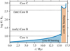 |
Fig. 1. Radius evolution of a 13 M⊙ star and definition of Case A, B, and C mass transfer. In this work, we also distinguish between early and late Case B, i.e. mass transfer starting immediately after a star finishes its main-sequence evolution and just before core helium burning, respectively. |
Here, we do not want to follow the complex binary mass-exchange phases, but focus on the effective outcome, namely the removal of the hydrogen-rich envelope and the consequence of this for the further evolution of stars up to core collapse. We remove the envelopes of stars in four evolutionary phases: towards the end of the main sequence when the central hydrogen mass fraction falls below 0.05 (Case A); shortly after the star leaves the main sequence and starts to cross the HR diagram (early Case B, often corresponding to stable mass transfer); shortly before the star ignites helium in its core (late Case B, often leading to unstable mass transfer, which is thought to result in a common-envelope phase); and after finishing core helium burning (Case C; often leading to unstable mass transfer that results in a common-envelope phase). Here we use the usual definition of early and late Case B mass transfer from donor stars with a radiative and convective envelope, respectively. However, we do not find systematic differences in early and late Case B binaries and therefore discuss them together as Case B stripped stars in the rest of the paper. In Fig. 1, we indicate these four cases for a 13 M⊙ star.
In our models, stars initially more massive than ≈20 M⊙ reach their maximum radius before the onset of core helium burning and therefore do not experience Case C mass transfer. Below, we nevertheless consider Case C envelope removal of such stars for completeness and clearly mark these stars in the rest of this work. However, massive RSGs are known to have extended atmospheres (e.g. Betelgeuse, O’Gorman et al. 2017) and so-called wind Roche-lobe overflow may increase the effective parameter space of Case C mass transfer (e.g. Podsiadlowski & Mohamed 2007; Mohamed et al. 2007; Abate et al. 2013; Saladino et al. 2018).
In practical terms, we remove the envelopes on a timescale of 10% of the thermal timescales of stars. This is a good assumption for Case B and C mass transfer given that Case B mass transfer is driven by the thermal-timescale expansion of the donor star and Case C mass transfer via common-envelope evolution is thought to be near adiabatic, that is, even faster than what we assume. Importantly, the chosen timescale for envelope removal is much faster than the nuclear evolution of stars, which means that their cores do not evolve chemically during envelope stripping. Applying an even faster timescale for envelope removal therefore results in almost the same pre-SN core structure (as is also exemplified by the almost indistinguishable pre-SN core structures of stars stripped in early- and late Case B mass transfer).
For Case A mass transfer, our assumption is less accurate and a robust relationship between the final stage after envelope removal and initial mass is not possible within our simplified modelling. Case A mass transfer proceeds via a fast, thermal-timescale mass-transfer phase followed by a slow, nuclear-timescale mass-transfer episode. During the latter episode, and possibly also during the subsequent Case AB mass transfer, a significant fraction of the envelope may be removed (e.g. Kippenhahn & Weigert 1967; Paczyński 1967; Wellstein et al. 2001). This sequence of envelope-removal episodes means that the core of the mass-losing donor can further evolve while its envelope is continuously being stripped off, and our simplified envelope-stripping model cannot properly reproduce this evolution. We try to avoid part of these complications by restricting our models to late Case A mass transfer. We stop the envelope removal once the surface hydrogen mass fraction falls below 1% for Case B and C mass transfer, and once the surface hydrogen mass fraction is less than 10% of that in the core for late Case A mass transfer.
2.3. Parametric supernova code
We compute explosion energies, compact remnant masses, nickel yields, and mean kick velocities for our single and binary star models using the parametric supernova model of Müller et al. (2016). Prior to shock revival, this model estimates the neutrino heating conditions based on semi-empirical scaling laws for the proto-NS radius, shock radius, the neutrino emission, and the neutrino heating efficiency. If the model indicates that shock revival occurs at some initial mass cut Mi before the gravitational neutron star mass exceeds the stability limit (here assumed to be  , i.e. a baryonic NS mass of about
 ![Mathematical equation: $ M_\mathrm{NS,by}^\mathrm{max}/{M}_{\odot}\approx M_\mathrm{NS,grav}^\mathrm{max}/{M}_{\odot} + 0.084 \cdot \left[M_\mathrm{NS,grav}^\mathrm{max}/{M}_{\odot}\right]^2 \approx2.336 $](/articles/aa/full_html/2021/01/aa39219-20/aa39219-20-eq2.gif) cf. Lattimer & Yahil 1989; Lattimer & Prakash 2001), the propagation of the shock and the growth of the explosion energy are followed through a phase of concurrent mass ejection and accretion. We account for energy input into the explosion by neutrino heating and explosive burning, and for the binding energy of matter swept up by the shock. Accretion and neutrino heating are assumed to stop once the post-shock velocity reaches escape velocity at some mass coordinate Mf. If the explosion energy drops to zero at some point after shock revival, or if accretion does not stop before the NS exceeds the maximum mass of 2.0 M⊙, we assume BH formation by fallback. The original model of Müller et al. (2016) does not predict the amount of fallback, and we therefore explore this parametrically.
cf. Lattimer & Yahil 1989; Lattimer & Prakash 2001), the propagation of the shock and the growth of the explosion energy are followed through a phase of concurrent mass ejection and accretion. We account for energy input into the explosion by neutrino heating and explosive burning, and for the binding energy of matter swept up by the shock. Accretion and neutrino heating are assumed to stop once the post-shock velocity reaches escape velocity at some mass coordinate Mf. If the explosion energy drops to zero at some point after shock revival, or if accretion does not stop before the NS exceeds the maximum mass of 2.0 M⊙, we assume BH formation by fallback. The original model of Müller et al. (2016) does not predict the amount of fallback, and we therefore explore this parametrically.
The mass ΔM = Mf − Mi and kinetic energy Ekin (which is approximately equal to the explosion energy Eexpl) of the post-shock matter at the “freeze-out” of accretion determine the NS momentum  , where the parameter α characterises the asymmetry of the neutrino-heated ejecta (Janka 2017; Vigna-Gómez et al. 2018). Although the degree of asymmetry is not universal (Janka 2017), a case can be made for a modest scatter in α due to the dominance of unipolar explosions (Katsuda et al. 2018; Müller et al. 2019), perhaps with a tail towards low α from explosions with bipolar geometry (Scheck et al. 2008; Müller et al. 2019). For simplicity, we assume a constant asymmetry parameter as in Vigna-Gómez et al. (2018) and compute the mean NS kick velocity vkick as
 (1)
(1)
where Mrm, grav is the gravitational mass of the compact remnant (either a NS or BH). The factor of 0.195 is a calibration factor chosen to match the best-fit σ of Hobbs et al. (2005) of σ ≈ 265 km s−1 (see Sect. 4.4). We note that the kick mechanism will result in kick velocities around the above computed mean value (Eq. (1)) with some dispersion. Here, we only consider the mean value and distributions thereof. In Appendix A, we show how Mi and ΔM are closely related to the two structural parameters of pre-SN models introduced by Ertl et al. (2016) to classify the explodability of stars.
We use a different calibration of the SN engine from that used in the original work of Müller et al. (2016). This is to obtain an average explosion energy of Type IIP SNe in the range 0.5 − 1.0 B (e.g. Kasen & Woosley 2009 suggest 0.9 B). The average explosion energy of Type IIP SNe is 0.69 ± 0.17 B (Sect. 4.3) for our chosen calibration parameters of the shock compression ratio, β = 3.3, and the shock expansion due to turbulent stresses, αturb = 1.22, (original values are β = 4.0 and αturb = 1.18; Müller et al. 2016).
3. Pre-SN evolution and structure
3.1. Single versus stripped binary stars towards core collapse
In massive single stars after core helium burning, the evolution of the envelope and the core decouple after the core has contracted and heated up sufficiently: there is a steep drop in pressure at the hydrogen–helium interface, where the hydrogen-burning shell is also located. The core no longer “feels” much of the hydrogen-rich envelope (e.g. in our initially 17 M⊙ single star at core helium exhaustion, the pressure drops from a mass coordinate of ≈6 M⊙ by more than ten orders of magnitude over 1 − 2 M⊙). The further core evolution and advanced nuclear-burning phases of (non-rotating) massive stars therefore essentially depend on the helium core mass MHe, the CO core mass MCO, and the amount of carbon left by helium burning XC. Here, XC and MCO are thought to be most relevant, to the extent that the evolution beyond helium burning is sometimes considered bi-parametric (e.g. Chieffi & Limongi 2020; Patton & Sukhbold 2020). Single stars populate a well-defined sequence in this MCO–XC plane (Fig. 2) as well as in the Mini–XC plane because of the one-to-one relation of MCO and Mini (Fig. 3).
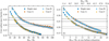 |
Fig. 2. Core carbon mass fraction XC as a function of (a) initial mass Mini and (b) CO core mass MCO at the end of core helium burning. The initial masses Mini of single stars corresponding to MCO are provided at the top of panel b (cf. Fig. 3). The light-grey shading indicates radiative core carbon burning and the darkish-grey shading indicates radiative core neon burning. The dashed (dotted) lines show the core carbon mass fractions at the end of core helium burning below which our models burn carbon (neon) in their cores radiatively. In panel b, we zoom in on the two branches and the ranges in XC and MCO do not correspond directly to those in panel a. |
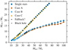 |
Fig. 3. CO core masses MCO at the core-helium exhaustion as a function of initial mass Mini of our single stars and the Case A, B, and C stripped stars. Models leading to BHs and likely experiencing significant fallback are indicated (see Sects. 4.1 and 4.2 for more details). |
The carbon abundance determines the strength of the ensuing carbon and later burning stages (e.g. Brown et al. 1996, 2001; Podsiadlowski et al. 2004; Chieffi & Limongi 2020; Sukhbold & Adams 2020). For example in our single stars, core carbon burning turns radiative for a carbon mass fraction XC ≲ 0.25 at core helium exhaustion and also neon burning turns radiative for XC ≲ 0.19. With a lower mass fraction of carbon and neon, the energy generated by carbon and neon burning can be mostly transported away by neutrinos such that no core convection develops1. We see below that radiative carbon and neon burning are indicators of the strength of advanced nuclear burning in general and hence the compactness of cores at core collapse.
Stars that lost their hydrogen-rich envelopes in Case A and B mass transfer reach conditions in terms of XC and MCO at the end of core helium burning that are genuinely different from those of single stars (Fig. 2). Consequently, their core evolution towards SN is also inherently different from that of single stars (see e.g. Timmes et al. 1996; Brown et al. 1996, 2001; Wellstein & Langer 1999; Podsiadlowski et al. 2004; Woosley 2019). By definition, Case C mass transfer leads to the same core conditions as in single stars at the end of core helium burning. However, this does not also automatically imply that the interior structure at core collapse is the same (see below). Also, the mapping from MCO to initial mass differs greatly in Case A and B stripped stars compared to single and Case C stripped stars (Fig. 3). This is particularly important when considering populations of stars, as we do below (cf. Fig. 2a).
We find that the early and late Case B models populate the same branches in the MCO–XC plane (Fig. 2) and also their pre-SN structures are almost indistinguishable. As outlined in Sect. 2.2, nuclear burning from our early to late Case B systems does not advance significantly during thermal-timescale evolution of the star. Analogously, our Case A and Case B models are also quite similar (e.g. in the MCO–XC plane), because we only consider late Case A mass transfer where the interior of the donor star is not too dissimilar to that of early Case B donor stars. However, we note that our Case A models are not capable of properly representing the distinct mass transfer episodes usually expected in Case A mass transfer (Sect. 2.2). Properly treating Case A mass transfer and considering earlier Case A systems than studied here is required to establish whether or not such stripped stars can populate another region in the MCO–XC plane and thus give rise to other pre-SN structures.
In our models, the two branches in the MCO–XC plane clearly persist up to core neon exhaustion and are still distinguishable by their different chemical compositions after core silicon burning. Because of this, stripped stars are expected to produce chemical yields that are systematically different from those of single stars, as we will show in a forthcoming publication.
The two branches in Fig. 2 can be understood as follows (see also Brown et al. 1996, 2001). During core helium burning, helium nuclei are first burnt into carbon and only at a later time is carbon converted into oxygen via the 12C(α, γ)16O reaction. In single stars, the convective, helium-burning core grows over time thanks to a hydrogen-burning shell that adds mass to the helium core (Fig. 4a). In contrast, the mass of the convective, helium-burning core of stars that have lost their hydrogen-rich envelope (and hence do not have a hydrogen-burning shell) stays roughly the same or even decreases2 during core helium burning (Fig. 4b). Consequently, there are fewer α-particles available to convert carbon into oxygen such that these stars have larger carbon abundances at the end of core helium burning.
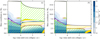 |
Fig. 4. Kippenhahn diagrams of core hydrogen and core helium burning of stars with an initial mass of 17 M⊙. The evolution of a genuine single star (panel a) is contrasted with that of a star that underwent (late) Case B mass transfer (panel b). The blue colour-coding shows energy production by nuclear burning, and the green, yellow, purple, and red hatched regions denote convection, thermohaline mixing, convective overshooting, and semi-convection, respectively. The blue and red dotted lines indicate approximate helium and carbon cores, here defined as the mass coordinate where the helium and carbon mass fractions first exceed 0.5. |
There are two further aspects that contribute to the two branches in Fig. 2 and to differences between stripped and single stars at core collapse. First, stars that have lost their hydrogen-rich envelopes are compact WR stars that lose mass at different rates compared to extended (super)giants. In particular, the winds directly decrease the mass of the helium cores. For example, this increases the carbon abundance at the end of core helium burning3 and may affect the central temperature and density. Moreover, this also applies to Case C stripped stars such that these models tend to have smaller helium core masses at core collapse than their single-star counterparts, which can induce differences in the pre-SN structure despite both models falling onto the same branch in Fig. 2 at the end of core helium burning. Secondly, the missing weight of hydrogen-rich envelopes reduces the pressure near the surface of stripped stars, and so their cores tend to evolve similarly to those of single stars with a slightly less massive helium core.
Because of these differences, the conditions for which carbon and neon burning turn radiative also change in Case A and B stripped stars (in Case C models we could not find differences with respect to single stars). Carbon burning proceeds under radiative conditions for XC ≲ 0.270 and neon burning for XC ≲ 0.205 at the end of core helium burning, while these limits are XC ≲ 0.250 and XC ≲ 0.190 in our single and Case C stripped stars. It is also evident from our models that the carbon abundance alone does not determine whether the ensuing carbon- and neon-burning phases are convective or radiative, but it is a combination of XC and MCO (see also Sukhbold & Adams 2020).
3.2. Pre-SN compactness, central entropy, and iron core mass
The different starting points for the advanced-burning stages of single and stripped stars shown in Fig. 2 persist up to the pre-SN phase. We highlight these differences by considering the compactness ξ2.5 ≡ ξM = 2.5 M⊙ (O’Connor & Ott 2011),
 (2)
(2)
the dimensionless central specific entropy sc, and the iron core mass MFe at core collapse (Figs. 5 and 6c). In Eq. (2), M is the mass coordinate at radius R(M) at which the compactness is measured. All three quantities are thought to be proxies for how likely it is that a star explodes successfully in a supernova. Stars with a small compactness parameter, low central entropy, and small iron core mass tend to be more explodable and form a NS.
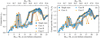 |
Fig. 5. Compactness ξ2.5 (panel a) and dimensionless central specific entropy sc (panel b) at core collapse as a function of CO core mass MCO. As in Fig. 2, initial masses Mini corresponding to the CO core masses of single stars are shown at the top (cf. Fig. 3), and the light-grey and darker-grey shadings are for radiative core carbon and core neon burning, respectively. |
The compactness ξ2.5, entropy sc, and iron core mass MFe are non-monotonic functions of MCO (Figs. 5 and 6c). We consider them as a function of MCO for easy comparison with the results in Sect. 3.1 and because MCO is a quantity that is relatively easily accessible and that is also often used for example in population-synthesis studies. They are mainly related to each other via the pre-SN (iron) core mass. The compactness is directly connected to the mass–radius relation of the “core”, as is the central entropy. The pre-SN iron cores have adiabatic profiles (i.e. sc = const.) such that they can be described by n = 3/2 polytropes. In such polytropes, the polytropic constant K scales as K ∝ M3R (P = Kρ(n + 1)/n) such that the entropy is s ∝ ln K ∝ 3ln M + ln R with the mass M and the radius R of the core. This implies that all three quantities qualitatively trace the same shape as a function of MCO, as can indeed be observed in Figs. 5 and 6c.
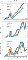 |
Fig. 6. Carbon-free (panel a), neon-free (panel b), and iron core mass (panel c) at core collapse as a function of CO core mass MCO. The carbon- and neon-free core masses are defined as those mass coordinates where the carbon and neon mass fraction falls below 10−5, i.e. these core masses (mass coordinates) indicate the bottom of the carbon- and neon-burning layers at core collapse. |
In our single stars and Case C mass-transfer systems, the compactness ξ2.5, entropy sc, and iron core mass MFe reach local maxima at MCO ≈ 7 M⊙ (Figs. 5 and 6c). All three quantities increase again for MCO ≳ 11 M⊙. The Case A and B stripped stars follow a similar, albeit shifted trend: the local maximum is now reached at MCO ≈ 8 M⊙ and only increases again for MCO ≳ 15 M⊙. Both, the local maximum, referred to as the “compactness peak” hereafter, and the increase in compactness for large MCO coincide with the transitions from convective to radiative carbon and neon burning, respectively.
Regardless of the exact explosion mechanism, these results show that there is an island of models around the compactness peaks of both the single and stripped stars where a successful supernova explosion is less likely. Similarly for large MCO (≳11 M⊙ for single and Case C stars, and ≳15 M⊙ for Case A and B stripped stars), it will become less likely that stars can explode. In the range MCO = 11 − 15 M⊙, Case A and B stripped stars at core collapse have significantly smaller compactness parameters and iron core masses than single stars, implying that they are more likely to explode. Consequently, stripped stars in this MCO range may lead to successful explosions and NS formation whereas single stars might not explode and produce BHs.
To further understand this non-monotonic behaviour, we consider the iron core masses as a function of MCO (Fig. 6). The total mass of the pre-SN iron cores is set by how fast the previous nuclear burning fronts move out in mass coordinate. Only those core regions that completed carbon, neon, oxygen, and silicon burning will constitute the iron core. The carbon- and neon-burning fronts in particular limit the growth of the iron cores as is illustrated in Fig. 6 by the carbon-free and neon-free core masses at core collapse (carbon- and neon-free being defined as those regions where the respective mass fractions are < 10−5; see also Fryer et al. 2002). Changes in the speed with which carbon and neon burning move out in mass coordinate lead to the iron-core-mass/compactness/central-entropy peak and the increase in MFe, ξ2.5 and sc at MCO ≳ 11 − 15 M⊙.
Interestingly, Patton & Sukhbold (2020) evolved bare CO cores of 2.5 − 10 M⊙ with initial carbon mass fractions of XC = 0.05 − 0.50 to core collapse and find a compactness landscape as a function of MCO and XC that qualitatively resembles our findings. The two branches of Case A and B stripped stars, and single and Case C stripped stars in Fig. 2, cross the compactness landscape of Patton & Sukhbold (2020) in different locations, just as the single and helium star models in their Fig. 6.
In conclusion, the cores of Case A and B stripped stars, and those of single and Case C stripped stars, evolve qualitatively similar up to core collapse. The SN outcome of single and Case C stripped stars will of course differ despite the similar core structures (e.g. SN type, the hydrogen-rich envelope that may affect the SN dynamics, etc.; see following section).
4. Core collapse and outcome
4.1. Compact-remnant masses
While the compactness parameter, the central entropy, and the iron core mass may be viewed as proxies of the explodability of stars, they cannot fully capture the outcome of the complex core collapse of stars (see e.g. Pejcha & Thompson 2015; Ertl et al. 2016; Müller et al. 2016; Burrows et al. 2020). Using the parametric SN code of Müller et al. (2016), we predict the likely outcome of core collapse of our models and show the resulting NS and BH masses as functions of initial mass Mini and CO core mass MCO in Fig. 7. We again use MCO as measured at the end of core helium burning to allow for direct comparisons with Figs. 2, 3, 5, and 6. The CO core masses at core collapse are slightly larger than MCO because of helium shell burning (on average 0.3%–1.4% and at most 7%).
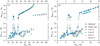 |
Fig. 7. Gravitational NS mass MNS, grav and BH mass MBH, grav as a function of the initial mass Mini of stars (panel a) and the CO core mass MCO (panel b). The large grey boxes indicate models with potential (here unaccounted for) fallback that may result in weak or failed SNe. The light yellow triangles are for models that have reached their maximum radius before core helium burning and thus cannot undergo Case C mass transfer. They are shown here mainly for completeness. |
In Fig. 7, we indicate those Case C systems that within our assumptions would not occur in isolated binary-star evolution because the donor stars reach their maximum radius before core helium burning (Sect. 2.2). We also mark models that may be able to launch an explosion by delayed neutrino heating, but where the energy input by neutrinos is not sufficient to expel the entire stellar envelope according to the semi-analytic SN model. A failed or weak supernova may result in significant fallback of envelope material onto the formed compact remnant. Such cases are found in both single and stripped stars beyond the respective compactness peaks.
The predicted NS and BH masses from stripped stars are on average less massive than those of single stars4 (when not considering the complications due to fallback). Most importantly, this is also true for single and stripped stars, even if they have the same CO core masses (Fig. 7).
In NS formation, stripped stars, on average, encounter SN shock revival in our models at smaller mass cuts Mi than single stars (Fig. 8a), which can be partly understood from their (on average) smaller iron cores (Fig. 6c). The initial mass cuts Mi are closely related to the final NS mass (cf. Figs. 7b and 8a), and this explains why stripped stars, on average, form lower NS masses. Also, the amount of mass involved in the accretion onto the proto-NS, namely ΔM = Mf − Mi, ultimately determines the overall neutrino luminosity and hence explosion energy (Fig. 8c). This mass ΔM is again larger, on average, in stripped stars than in single stars (Fig. 8b, excluding the fallback cases), so stripped stars will generally give rise to more energetic SN explosions than single stars. We come back to this and further consequences for the kicks and nickel yields in Sects. 4.3 and 4.4.
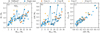 |
Fig. 8. Initial mass cut Mi of SN shock revival (panel a) and mass ΔM = Mf − Mi involved in accretion onto the proto-NS star (see Sect. 2.3) as a function of MCO (panel b), and the resulting SN explosion energy Eexpl as a function of ΔM (panel c). The final NS mass correlates strongly with Mi (cf. Fig. 7b). The vertical dotted line in panel a is the assumed maximum (baryonic) NS mass. |
We also note that Mi and ΔM are closely related to the mass coordinate of the base of the O shell, M4, and the spatial mass derivative at this point, μ4, respectively (Appendix A), that is, to the two structural parameters of pre-SN models that Ertl et al. (2016) found to be good predictors of the explodability of stars. In conclusion, stripped stars tend to be “easier” to explode than single stars.
In BHs, the lower masses from stripped stars compared to single stars (Fig. 7) are rather straightforward to understand as the BH mass is given by the total final mass of stars. This mass is lower in stripped stars that lost their hydrogen-rich envelopes than in single stars (Case A stripped stars produce the lowest final masses, followed by Case B and Case C systems; for the possibility of a partial ejection of the hydrogen envelope; see Sect. 6.3).
The compactness peaks described in Sect. 3.2 (Fig. 5a) result in islands of BH formation (Fig. 7). These islands are at different masses for single stars and Case A and B stripped stars, analogously to the shifted compactness peaks. While single stars of initially ≈22 − 24 M⊙ produce BHs of ≈13 M⊙ because of the compactness peak, Case A and B stripped stars do so for initial masses of ≈32 − 35, M⊙ and give rise to BHs of ≈9 M⊙ (see also Table 1). Therefore, single stars in the compactness peak produce BHs whereas stripped stars with the same CO core mass would produce NSs and vice versa.
Initial mass ranges for NS formation in our single and stripped binary star models.
Single stars of initially ≳35 M⊙ produce BHs of ≳17 M⊙ in our models (Fig. 7 and Table 1). Because envelope stripping tends to make stars more likely to explode, our Case A and B stripped stars may produce BHs only for initial masses of ≳70 M⊙ (MCO ≳ 15 M⊙). This is connected to the relatively moderate compactness parameters of Case A and B stripped stars up to MCO ≈ 15 M⊙ as shown in Fig. 5a. However, our analysis indicates that fallback may occur in some of the stripped stars in the CO core mass range 9 − 15 M⊙ such that these stars may then produce BHs. The same is true for single stars beyond the compactness peak, and on average 20%–40% of our models beyond the compactness peak experience fallback and a weak/failed SN. In conclusion, stripped stars produce NSs over a larger range of initial masses and, even more importantly, over a larger range of CO-core masses than single stars (Table 1).
There is a mass gap between NSs and BHs at about 2 − 9 M⊙ (Fig. 7). This gap exists because the applied SN mechanism only has two outcomes: successful explosion or formation of a BH. With partial fallback of envelope material, the gap could be narrowed or even filled completely. We come back to this in the following section (see also discussion in Sect. 6.4).
4.2. NS–BH mass distribution
We next construct NS and BH mass distributions for stellar populations born in a single starburst at solar metallicity (Fig. 9). These distributions cannot be directly compared to compact-object mass distributions from gravitational-wave observations for example, because the latter will be a mixture of stars of different metallicities formed according to the cosmic star-formation history.
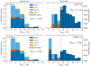 |
Fig. 9. Mass functions of NSs and BHs in our default model (top panel) and a model accounting for fallback (bottom panel). The vertical lines show the median masses of the NS and BH mass distributions, and the corresponding values are provided in the figure. Possible LBV phases are only indicated for the single stars. |
To set up the population, we assume that the initial masses of stars (in binaries, the more massive primary star M1) are distributed according to a power-law initial-mass function with a high-mass slope of γ = −2.3 (Salpeter 1955; Kroupa 2001; Chabrier 2003). The primordial binary fraction is set to 70%, and uniform distributions of mass ratio q = M2/M1 and logarithmic orbital separation log a are used (M2 is the initial mass of the secondary star). Orbital separations are limited to log a/R⊙ ≤ 3.3 (a ≲ 2000 R⊙). For Case A, B, and C mass transfer, we assume that binaries merge and thus do not result in a stripped star if q < 0.5, q < 0.2, and q < 0.2, respectively (cf. Schneider et al. 2015). We only consider genuine Case C systems. Accounting for all binary interactions (mass losers, mass gainers, mergers, and CE systems), about 70% of all stars in our population interact by mass exchange in a binary and 30% evolve as effective single stars, similarly to what is expected in Galactic O stars (Sana et al. 2012).
In our sample, there are no stars that may explode in electron-capture supernovae (ECSNe). Such SNe have been suggested to produce rather small NS masses of ≈1.25 M⊙ (e.g. Podsiadlowski et al. 2004; van den Heuvel 2004; Schwab et al. 2010), but these are missing in our distributions. Also, we only consider one binary-mass stripping episode, where additional such episodes can occur and may lead to ultra-stripped stars that could then again give rise to low-mass NSs (maybe as low as 1.1 M⊙; see Tauris et al. 2015). The lowest baryonic iron core mass in our sample is 1.49 M⊙ and the lowest gravitational NS mass is 1.32 M⊙. In Sect. 4.2.1, we first discuss the compact-object mass distributions of our default stellar-remnant masses (Fig. 7), and in Sect. 4.2.2 we then also consider partial fallback.
4.2.1. Default model
First, we describe the results of the genuine single stars (Fig. 9 top panel). Their NS masses follow a unimodal distribution with a tail up to 1.9 M⊙ (the largest NS mass in the single-star sample is 1.87 M⊙). The maximum allowed NS mass in this study is 2.0 M⊙, but this is not reached by stars in our grid of models. A finer grid is probably required to sample the NS mass distribution up to the highest masses. In any case, some NSs are born massive in our models, in agreement with pulsar observations (e.g. Demorest et al. 2010; Lin et al. 2011; Tauris et al. 2011). High individual NS masses are also inferred in the compact-object merger GW190425 with a total mass of ≈3.4 M⊙ (Abbott et al. 2020a).
The NS-mass distribution has a gap or dearth at 1.6 − 1.7 M⊙ (Fig. 9a), which is caused by stars in the compactness peak for which we predict BH formation (see the “BH island” at MCO ≈ 7 M⊙ in Fig. 7 and the corresponding compactness peak in Fig. 5a). Whether the NS mass distribution shows a gap, dearth, or other feature because of the compactness peak also depends on the NS masses of other stars (see Appendix C): for example, there is no gap or dearth if stars beyond the compactness peak give rise to NS masses that are lower than those of stars before the compactness peak.
The BH-mass distribution of single stars is bimodal (Fig. 9b). The first peak at ≈12.5 M⊙ is from stars in the compactness peak that failed to explode. The second, major contribution to the BH-mass distribution starts at a BH mass of ≈17 M⊙. This mass is set by the final mass of the lowest-mass single star beyond the compactness peak that fails to explode. This mass is mainly set by the total (wind) mass loss of a star, which implicitly depends on the exact evolutionary history of the star and parameters such as convective-boundary mixing (e.g. convective overshooting). The most massive BH in our sample (≈50 M⊙; not visible in Figs. 7 and 9) is given by the final mass of the most massive single star that we evolved up to core collapse (here 75 M⊙). It is possible for this to be larger than what we have in our current sample, but our models do not include mass loss during LBV phases or other forms of pulsational and eruptive mass loss from massive stars (see e.g. Smith 2014), which likely limits BH masses from single stars.
We indicate stars that potentially experience LBV-like mass loss by the black hatching in Fig. 9 and their compact remnant masses should rather be considered as upper limits. Stars are indicated to undergo enhanced mass loss if they cross the hot side of the S Doradus instability strip (e.g. Smith et al. 2004) or a luminosity of log L/L⊙ = 5.5 (Davies et al. 2018) for effective temperatures Teff < 14, 350 K, such as for example RSGs.
The NS and BH mass distributions of stripped stars show qualitatively similar features to those of genuine single stars. However, there are important quantitative differences. First, the compactness peak is at larger CO core masses and does not result in a very pronounced dearth in the NS mass distribution (Fig. 9a). The gap in the NS mass distribution produced by the compactness peak in single stars is now filled with NS from stripped binary stars.
Secondly, the NS masses of stripped stars are on average smaller than those of single stars (see also Fig. 7b). The average NS mass of our stripped binary models is ≈1.42 M⊙, while it is ≈1.46 M⊙ in the single star models. This systematic difference is further exemplified by the NS mass distribution of stripped binary stars that peaks at ≈1.35 M⊙ while that of single stars peaks at ≈1.45 M⊙. From our models, it also seems that the NS mass distribution of stripped stars is effectively truncated at about 1.6 M⊙, whereas that of single stars extends up to 1.9 M⊙. The NSs born with masses ≳1.6 − 1.7 M⊙ in the single and stripped stars are from stars close to the transitions from NS to BH formation. Because these transitions are at lower initial masses for single stars, there are relatively more such massive NSs because of the IMF and a more pronounced tail is formed towards large NS masses.
Thirdly, the maximum BH mass of stripped stars in our sample is ≈20 M⊙ compared to ≈50 M⊙ in single stars (Fig. 9b). This maximum mass could be slightly larger when considering stripped binary models from initially > 100 M⊙ stars. Also, the contributions of BHs from stars in and beyond the compactness peak, that is, BH masses of ≈9 M⊙ and ≳15 M⊙, respectively, are lower in stripped stars in comparison to single stars with ≈12.5 M⊙ and ≳17 M⊙, respectively. The main difference in the masses is of course due to the stripped envelope in the binary models.
There are no BHs in the mass range ≈2.0 − 8.7 M⊙ in our default model of stripped binary stars (Fig. 9 top panel). As mentioned above, this is because in our SN model, we assume either a complete explosion without any fallback or no explosion with total fallback of the whole final stellar mass. We relax this assumption in the following section.
4.2.2. Fallback model
Within the applied SN model, we encounter cases where an explosion is triggered, but it is then not energetic enough to explode the whole star (the fallback cases in Fig. 7). We now assume that 50% of the presumed ejecta mass falls back and is added to the compact remnant mass. Black holes are produced instead of NSs.
The fallback narrows down the mass gap between NSs and BHs from ≈2.0 − 8.7 M⊙ to ≈2.0 − 5.4 M⊙ (Fig. 9 bottom panel). A smaller fallback fraction leads to lower compact-object masses (i.e. BHs) and therefore leads to a narrowing of the gap. Viceversa, a larger fallback fraction would widen the gap. In principle, the gap could disappear altogether, in particular if various fallback fractions are realised in nature.
The main characteristics of the NS and BH mass distributions (cf. Sect. 4.2.1) remain intact otherwise; for example, stars in the compactness peak still make a distinct contribution to the BH distribution and may lead to a dearth in the NS distribution. Because the fallback BHs stem from on average lower initial masses than other BHs, they add a significant contribution to the BH mass distribution at ≈5.0 − 8.0 M⊙, that is, they are the least massive BHs in our models. This contribution is larger than that from BHs formed from stars in the compactness peak. While not immediately visible in Fig. 9d, the lowest-mass fallback BHs are still from stripped stars, but this may no longer be true when considering that different stars may experience varying levels of fallback.
4.3. Explosion energy and nickel mass
As described in Sect. 2.3, we re-calibrated the parametric SN code of Müller et al. (2016) such that the average explosion energy of SN IIP is 0.69 ± 0.17 B (stripped binary models do not contribute to this calibration). Using the same population model as in Sect. 4.2, we show the distribution of explosion energies of our single and stripped binary stars in Fig. 10a. The average explosion energy of SN Ib/c is 0.88 ± 0.31 B (almost exclusively stripped binary stars) and is systematically larger by 28% than that of SN IIP.
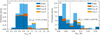 |
Fig. 10. Distribution of (a) explosion energies and (b) nickel masses of single and stripped binary stars. |
The more energetic explosions of stripped stars in our models are a consequence of the larger mass ΔM that is accreted onto the NS and powers the neutrino luminosity (Fig. 8c), as discussed in Sect. 4.1. Another often-used proxy for the explosion energy is the compactness parameter ξ2.5 (Fig. 11a; see also Nakamura et al. 2015; Müller et al. 2016), but it appears to be of limited use in our models. We find that models with ξ2.5 ≲ 0.15 have a similar explosion energy of about 0.75 B and that there is an approximately linear trend of explosion energy with compactness for ξ2.5 ≳ 0.15. However, the scatter around this general trend is large and precludes the use of the compactness as a predictive quantity for explosion energy. For ξ2.5 ≲ 0.40, we exclusively find SN explosions, while both successful and failed SNe are possible for more compact stars.
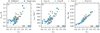 |
Fig. 11. Explosion energy (a), kick velocity (b), and nickel mass (c) as a function of compactness. |
More energetic explosions also result in larger nickel yields (Fig. 10b) and SN kicks (Sect. 4.4) as is also evident from the general correlations of compactness with nickel yield and SN kick velocity (Fig. 11). The correlation of nickel yield and compactness shows the least scatter. This suggests that the nickel yields from observations could shed light on the compactness of an exploding star, although further investigation with more detailed SN models is warranted.
Because of the more energetic explosions of stripped stars, we find that SN Ib/c produce on average 0.059 M⊙ of nickel, while SN IIP produce on average 0.039 M⊙. Taken together, we find an average nickel yield of 0.049 M⊙ (Fig. 10b). Higher nickel masses in more energetic explosions can be understood as follows. The higher explosion energies lead to higher shock temperatures over a larger range in the stellar interior, which enables more nuclear burning, producing more nickel.
4.4. NS and BH kicks
As in Sect. 4.2 and 4.3, we compute the distribution of the mean SN kick velocities from our population of single and stripped binary models. We consider the default and fallback cases separately (Fig. 12). In the fallback case, we assume that the NS of mass MNS has received a kick of vkick before it accretes fallback material. The new kick of the compact object (most likely a BH) then follows from linear momentum conservation,
 (3)
(3)
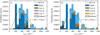 |
Fig. 12. Supernova-kick distribution of all stars without (panel a) and with (panel b) fallback. Maxwellian distributions are fitted to the data, and their best-fit σ values are provided. |
where Mfallback is the amount of fallback mass. As detailed in Sect. 4.2.2, we here assume that the fallback material is 50% of the original ejecta mass.
We note that all our kick velocities are mean values and do not take the stochastic nature of SN kicks into account (see Sect. 2.3). Also, the kick velocities in Fig. 12a are calibrated to match the observed distribution of Hobbs et al. (2005), which is a Maxwellian distribution with σ = 265 km s−1. In our models, the kick velocity scales directly with explosion energy, the matter involved in the accretion onto the proto-NS, and the mass of the NS itself, (Eq. (1)),  . Our previous findings of on average higher Eexpl, larger ΔM, and smaller MNS, grav in stripped stars compared to single stars immediately imply that also the kicks within our SN model are on average larger in stripped stars, as shown in Fig. 12.
Quantitatively, mean kick velocities are in the range 180 − 1500 km s−1 (50 − 1500 km s−1) without (with) fallback. The best-fitting Maxwellian distributions are for σ = 222 ± 23 km s−1 and σ = 315 ± 24 km s−1 in single and stripped stars, respectively5.
When plotting the kick velocity against the compactness of pre-SN stars, we see the same qualitative trend as found in the explosion energy (Fig. 11b): successful explosions from stars with a higher compactness lead to larger explosion energies and hence kick velocities. Analogously to the explosion energies, the largest kicks are found in stripped binary stars and almost all kicks larger than 600 km s−1 are from stripped binary models.
Models likely experiencing fallback are marked in Fig. 12 and all of the BHs formed by fallback in our models receive (mean) kick velocities in the range ≈50 − 150 km s−1, which is significantly slower than most of the kick velocities of NSs. As shown in Sect. 4.2.2, the fallback BHs populate the mass gap between NSs and non-fallback BHs. In our models, fallback BHs would always receive a kick, which might not be the case for more massive BHs that may form by direct collapse. If the fallback fraction is less than 50% of the ejecta mass, the final mass of the compact remnant will decrease and the kick velocity will increase (and vice versa). For a distribution of fallback fractions as might be expected in reality, this implies that the average kick velocity would decrease with increasing BH mass.
5. Compact-object populations and merger statistics
Using a toy population-synthesis model, we now study how binary-mass stripping may affect compact-object populations and particularly merger rates. The toy model is meant to be simple and to offer guidance on the expected order-of-magnitude changes in NS–NS, BH–NS, and BH–BH merger rates caused by envelope stripping in binary stars; it will not be able to properly catch all of the complex intricacies of a full population-synthesis computation, which is left for future work. For example, we only consider a single starburst population of stars of solar metallicity without accounting for the cosmic star-formation history. Metallicity-dependent stellar winds directly affect the final masses of stars and possibly also the SN outcome, and the masses of compact objects are important for the detection rates of merger events. We describe the population setup and assumptions in Sect. 5.1, compare a few population predictions to Galactic compact objects in Sect. 5.2, and present our findings on compact-object merger rates in Sect. 5.3 and chirp-mass distributions in Sect. 5.4.
5.1. Toy population model
A typical binary system leading to a double compact-object merger within a Hubble time undergoes the following key steps, which we try to capture in our population model: The first mass transfer episode (e.g. Case B) from the primary to the secondary star is stable. The primary star is stripped of its envelope, directly modifying its core evolution and hence compact-object remnant as shown in this work. The secondary star accretes mass and rejuvenates. If the binary survives the first SN kick, it may undergo a second mass-transfer phase that may now be unstable and lead to a common-envelope phase. During this phase (and possibly thereafter in another mass-transfer episode), the initial secondary star is also stripped of its envelope with consequences for its final fate and compact remnant. During the common-envelope phase, the orbit greatly shrinks and the binary star has a greater chance of surviving the kick from the second SN. Ultimately, the two compact objects merge in a Hubble time thanks to gravitational-wave emission. Such a channel makes up about 70% of NS–NS mergers in the models of Vigna-Gómez et al. (2018).
As in Sect. 4.2, primary-star masses M1 are sampled from a power-law IMF with γ = −2.3 and secondary-star masses from a uniform mass-ratio distribution (the minimum companion mass is 1 M⊙). Initial masses are limited to Mmax = 70 M⊙ to account for the fact that wind mass loss and enhanced mass loss from LBV-like eruptions and pulsations widen orbits such that binary systems no longer experience mass exchange (e.g. Vanbeveren 1991; Schneider et al. 2015). For the same reason, we limit BH masses for our solar metallicity models to 25 M⊙. Orbital separations are limited to log amax = 3.3 as before and are sampled from a uniform distribution in log a. We assume that binary stars undergoing Case A mass transfer do not contribute to compact-object mergers and thus only consider Case B and C systems. This is because the orbital periods after Case A mass transfer are rather short and the subsequent common-envelope phase likely leads to a merger (e.g. Terman et al. 1995). After the first mass-transfer episode from the primary to the secondary star, we assume that the secondary accretes 40% of the mass of the primary star and that it rejuvenates in the sense that its evolution after mass accretion can be well described by its new total mass. We do not follow the exact orbital evolution of binary stars, also not through common-envelope phases.
The initial mass ranges for white dwarf (WD) and NS formation are different in single and binary-stripped stars, and are closely connected to the occurrence of ECSNe6. In single (stripped) stars, we assume WD formation for Mini < 9.5 M⊙ (Mini < 10.5 M⊙). Also, the initial mass range of ECSNe is expected to be different in stripped binary stars compared to single stars (e.g. Podsiadlowski et al. 2004; Tauris et al. 2017; Poelarends et al. 2017). We assume that single stars give rise to ECSNe for initial masses in the range 9.5 − 10.0 M⊙, while this mass range is 10.5 − 12.0 M⊙ in stripped binary stars. The exact mass ranges are currently uncertain, which we find to be important in particular for the NS–NS merger rate. Here, we want to capture the general expectation that stripped binary stars likely produce ECSNe over a larger initial mass range than single stars and that higher initial masses are required because of envelope stripping.
Supernova kicks are a key (yet considerably uncertain) ingredient in predicting compact-object-merger rates (e.g. Giacobbo & Mapelli 2018). Within our toy model, we reduce the number of binaries that can lead to compact-object mergers for each kick and apply different reduction factors depending on whether NSs or BHs are formed. For NSs formed in ECSNe, we assume that binaries are not disrupted. For NSs formed in CCSNe, the first and second SNe are assumed to break up 90% and 20% of binaries, respectively. The latter two fractions are average values reported by Vigna-Gómez et al. (2018) in their more detailed population-synthesis work. Renzo et al. (2019) report a similar break-up fraction of  for the first SN in a binary system. For BHs, we assume that 20% break up at the first SN and that none break up at the second. If the BH formed by fallback, we increase the break-up fraction to 40% for the first SN.
In our models we find that 20%–40% of stars beyond the compactness peak may experience fallback and thereby BH formation. We therefore assume that one-third of models beyond the compactness peak that may form NSs will experience fallback of 50% of the ejecta mass (as assumed in Sect. 4.2.2).
Initial masses are related to CO core masses and hence NS and BH masses through fitting formulae to our single-star, and Case A, B, and C stripped binary-star models (Fig. 3 and Appendix B). Neutron stars from ECSNe are all assumed to have a mass of 1.25 M⊙ (Schwab et al. 2010). Below, we also consider the rapid and delayed supernova model of Fryer et al. (2012) for comparison, because it is regularly employed in state-of-the-art population-synthesis computations of gravitational-wave sources (e.g. in StarTrack, Belczynski et al. 2020, Compas, Stevenson et al. 2017, and MOBSE, Giacobbo & Mapelli 2020), but there are also other population-synthesis models that use different prescriptions (e.g. COMBINE, Kruckow et al. 2018).
In our population model, we make the implicit assumption that compact-object mergers form similarly from binaries with different primary star masses (i.e. the progenitors of NS–NS and BH–BH mergers follow the same evolutionary paths). Qualitatively, this may be a valid assumption, but it may not necessarily hold quantitatively. For example, the fraction of binary systems experiencing an unstable first mass-transfer episode likely decreases with primary mass, implying that the fraction of binary systems undergoing CE evolution is lower in more massive primary stars (see e.g. Schneider et al. 2015). Our toy model captures part of this, because the available parameter space for Case B and C mass transfer is smaller in more massive primary stars. Furthermore, we do not include the close binary channel invoking chemically homogenous evolution for the formation of massive BH–BH mergers (Mandel & de Mink 2016; Marchant et al. 2016) in our toy model, and also not dynamical formation channels (e.g. Rodriguez et al. 2015; Mapelli 2016; Banerjee 2017).
In the following, we make a differential analysis and only consider relative quantities. In particular, we consider the following models that mainly differ in their mapping from initial to compact-remnant masses:
Single. The final fate (i.e. ECSN, CCSN, and NS or BH formation) and the compact remnant mass of the primary and secondary stars in binaries are defined by our single star models (see Figs. 3 and B.1a). This assumption is known to be particularly invalid and is considered here only for reference.
Default. This is our default model. We map the initial masses of stars to CO core masses and then to compact-object masses using our Case B models (see Figs. 3 and B.1c).
CPS. This and the following two models are our attempt to mimic what is done in current population-synthesis (CPS) models. As in our default model, we map the initial masses of the primary and secondary stars to CO core masses using our Case B stripped binary star models, but we map the evolution from CO core mass to final fate (e.g. NS or BH formation) according to our single-star models. If a NS is formed, we use the NS mass predicted by the single-star mapping, and BH masses are equal to the final mass of the Case B stripped model.
F12 rapid. This model resembles the CPS model, but the mapping from pre-SN CO core mass to compact remnant mass resembles that of the rapid explosion model described in Fryer et al. (2012).
F12 delayed. This model resembles the F12 rapid model, but uses the delayed explosion model of Fryer et al. (2012).
5.2. Comparison to Galactic compact objects
In Table 2, we summarise a few key quantities of the models described in Sect. 5.1. The NS-to-BH ratio is computed for stars initially up to 100 M⊙. The NS-to-BH ratio in our stripped-binary models is significantly higher than in the single-star models and the two F12 models. This is because the envelope stripping in our binary models greatly extends the initial-mass range over which NS (and not BH) formation is found (Table 1). While the differences in the NS to BH ratios are large, they appear less so when considering the fraction of NSs among all NSs and BHs (NNS and NBH being the number of NSs and BHs, respectively):
 (4)
(4)
Fractions of NSs to BHs (fNS/BH), single NSs ( ), single BHs (
 ), single radio pulsars (
 ), single recycled pulsars (
 ), double-neutron-star (DNS) systems with at least one NS formed in an ECSN (
 ), and NSs in binaries after the first SN (
 ) in the considered toy population models.
for fNS/BH = 3 − 15 (Table 2). In particular, the NS fraction is only 3% higher in our default stripped binary model (94%) than in the CPS model (91%), despite the relatively large difference in the NS-to-BH ratio and the fact that about one-third of the BHs in the CPS model are NSs in the default model.
In all models, NSs are mostly single (≳80% of all NSs) because of the SN kicks, while about half of all BHs are single and the other half is in binary systems with another compact object (Table 2). In particular, we consider the fraction of single radio pulsars to be a key benchmark for SN kick prescriptions in population-synthesis models. We define NSs as radio pulsars if they are not expected to have accreted mass (e.g. all second-born NSs). Analogously, we define NSs as recycled if they likely accreted mass during their lifetime (e.g. the first-born NSs in binaries that are not broken up by kicks). In all models, about 90% of radio pulsars are single, which appears to be in broad agreement with observations (J. Antoniadis & M. Kramer, priv. comm.). About 15%–20% of all recycled pulsars are single given our SN kick assumptions, which is an interesting prediction that could be tested against future observations.
The NS–NS merger rate relates directly to double NS systems. In about 70% of these, at least one NS formed in an ECSN in our toy population (or more generally in a low-kick SN; Table 2). This is because we assume that binaries are not broken up by ECSNe. Tauris et al. (2017) compile a list of 13 double NS systems of which six systems have known component masses. Four of these systems have one NS with a mass of < 1.3 M⊙ and a rather moderate eccentricity (e < 0.1 − 0.2). From this information, we infer that roughly two-thirds (67%) of known double-NS systems have at least one NS that formed in a low-kick SN (e.g. an ECSN or from a low-mass iron core progenitor, hence the low NS mass and moderate eccentricity). These statements are based on low-number statistics and should not be over-interpreted, but provide credibility to our assumed kick prescriptions and mass range for ECSNe from stripped binary stars.
A direct consequence of these assumptions is that many if not most NS–NS mergers in stripped binary populations are related to low-kick SNe and the mass range over which they form. Binary break-up fractions and the size of the parameter space from which low-kick SNe may be expected (e.g. ECSNe; Podsiadlowski et al. 2004; Poelarends et al. 2017) are therefore probably a significant source of uncertainty in the NS–NS merger rates of more elaborate population-synthesis models and warrant further investigation.
5.3. Compact-object merger rates
Here, we consider the intrinsic merger rates of compact objects in our toy population model and also estimate detection rates. For the latter, we consider the signal-to-noise ratio (S/N) of a merger event in a single gravitational-wave detector; it is higher for a larger redshifted chirp mass, Mchirp(1 + z) (where z is the redshift), and a closer (luminosity) distance to the source, dL, (e.g. Finn & Chernoff 1993; Finn 1996),
![Mathematical equation: $$ \begin{aligned} S/N \propto \frac{1}{d_\mathrm{L} }\left[ M_\mathrm{chirp} (1+z) \right]^{5/6}. \end{aligned} $$](/articles/aa/full_html/2021/01/aa39219-20/aa39219-20-eq22.gif) (5)
(5)
The chirp mass Mchirp = (m1m2)3/5/(m1+m2)1/5 is directly measured from the frequency evolution of the gravitational-wave signal and is larger for more massive component masses m1 and m2. Merger events with a larger chirp mass (e.g. BH–BH mergers) therefore result in a higher S/N and are observable over a larger volume or fraction of the Universe. For a fixed S/N, dL ∝ (Mchirp)5/6 such that the observable volume Vobs ∝ (dL)3 ∝ (Mchirp)5/2. To first order, we therefore expect that the rates of compact-object mergers R ∝ (Mchirp)5/2 (see also Finn & Chernoff 1993; Finn 1996). Below, we use this scaling of the merger rates with chirp mass to estimate the detection rates of gravitational-wave merger events (this does not take into account the frequency dependence of the sensitivity curve of the detector).
Changes in the intrinsic merger rates of NS–NS, BH–NS, and BH–BH with respect to our default population model are shown in Fig. 13a (ΔRx = [Rdefault − Rx]/Rx, i.e. positive [negative] differences are for higher [lower] merger rates in the default model with respect to a comparison model x). As expected from the NS-to-BH ratio (Table 2), the NS–NS merger rate is intrinsically the highest in our default model. When considering the detected NS–NS merger rate, the CPS model has a higher NS–NS merger rate than the default model, because the NS masses and hence the chirp masses are on average smaller in the stripped binary models than in the single star models employed in the CPS model.
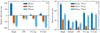 |
Fig. 13. Expected changes of intrinsic gravitational-wave merger rates ΔR of our default model with respect to the single, CPS, F12 rapid, and F12 delayed models (panel a), and ratios of detection rates (panel b). The rate differences ΔR are defined such that positive (negative) values imply a higher (lower) rate in our default model compared to the other models. |
It is not only the bare NS-to-BH ratio that sets the formation rate of NS–NS mergers, but also the number of NSs that receive such kicks that binaries are not broken up. Hence, low-kick SNe such as ECSNe can make a big difference: for example, restricting the initial mass range for the occurrence of ECSNe in our default model (10.5 − 12.0 M⊙) to the same as that used in the single-star population model (9.5 − 10.0 M⊙) would reduce the NS–NS merger rate by about 60% despite the now lower initial mass threshold for the formation of NSs. This also explains a large part of the difference in the NS–NS merger rate between our single and default population models. Also, the larger intrinsic NS–NS merger rate of our default model in comparison to the CPS (2%), the F12 rapid (6%), and the F12 delayed models (15%) is due to the larger NS-to-BH ratio (Table 2), as we apply the same assumptions on ECSNe in these models.
The intrinsic and detected7 BH–NS and BH–BH merger rates are the lowest in our default model (Fig. 13a). In particular, the BH–BH merger rate can be lower by even an order of magnitude (ΔR ≈ −90% with respect to the F12 rapid and delayed models) when considering that our stripped binary stars produce NSs rather than BHs over a large initial-mass range (Sect. 4.1). Even the seemingly small difference in the mapping from CO core masses to NS or BH formation between our default and the CPS model (i.e. shifted compactness peak and BH formation at smaller compactness in the single star models with respect to the stripped envelope models) leads to a decrease in the intrinsic BH–NS and BH–BH merger rates by about one-quarter. We note again that our toy population lacks a potential contribution from BH–BH mergers from stars evolving chemically homogenously in close binaries and in dense stellar systems such as star clusters.
Within a differential analysis, we next consider the merger-rate ratios RBHBH/RNSNS, RBHNS/RNSNS, and RBHBH/RBHNS. These ratios are a promising way to compare models to gravitational-wave observations because the individual ratios are influenced in different ways by certain physical mechanisms. Here, we focus on the question of how the pre-SN structures relate to NS and BH formation. The single-star model clearly stands out with the highest rate ratios. The merger rate ratios are so high because of the relatively low NS-to-BH ratio (Table 2), the limited initial-mass range of NS formation in low-kick SNe (here ECSNe), and the larger average BH masses of the single-star models compared to the stripped-binary models. The latter leads to larger chirp masses and therefore higher detection rates.
In the F12 rapid and delayed models, the individual BH masses are smaller than those in the single-star models because of envelope stripping. Therefore, the chirp masses of mergers involving BHs are also smaller and thereby the detected BH–BH and BH–NS merger rate. At the same time, the NS–NS rate is increased due to the larger contribution of NSs from low-kick SNe (here ECSNe). Together this drastically reduces the RBHBH/RNSNS and RBHNS/RNSNS merger-rate ratios (Fig. 13b). The ratio RBHBH/RBHNS stays about the same because the NS-to-BH ratios are quite similar in the three models (Table 2).
Comparing the F12 rapid and delayed models to our default and CPS models, the initial-mass range for NS formation is larger in the latter models such that fewer BHs are formed. As shown in Fig. 13a, this decreases the intrinsic BH–BH and BH–NS merger rates and increases the NS–NS merger rate. Consequently, RBHBH/RNSNS and RBHBH/RBHNS decrease and RBHNS/RNSNS remains about the same in our toy population model (Fig. 13b). To fully understand this picture, we note that the F12 rapid and delayed models predict more lower-mass BHs than our default and CPS models such that they contribute relatively less in the detected merger rates involving BHs. For example, this explains why the intrinsic BH–BH merger rate is almost a factor of ten higher in the F12 models than in our default model but the detected RBHBH/RNSNS ratio is only a factor of approximately six larger.
5.4. Chirp-mass distribution
In the following, we compute chirp-mass distributions of NS–NS, BH–NS, and BH–BH mergers from their detection rates8. In particular, we highlight characteristic features that can be directly linked to our models of stripped binary stars.
The chirp-mass distribution of the default, CPS, and the F12 models are shown in Fig. 14a. In Fig. 14b, we only show results for the default model with switched-off fallback to highlight the most important features. The chirp-mass distribution is multi-modal and there are three main components from NS–NS, BH–NS, and BH–BH mergers at logMchirp ≈ 0.1, ≈0.5 and ≈1.0 that are further split into sub-components (Fig. 14b). To help understand these features, we recall that the compact-object masses from our stripped binary models without fallback (stripped star contribution in top panel of Fig. 9) are split into three main groups: NSs (≈1.4 M⊙), lower-mass BHs (BHL; ≈9 M⊙) from stars in the compactness peak, and higher-mass BHs (BHH; ≈17 M⊙). Mergers of compact objects from these three groups then explain the six components observed in Fig. 14b:
-
The NS–NS contribution at logMchirp ≈ 0.09;
-
The two BH–NS contributions at logMchirp ≈ 0.46 (BHL + NS) and logMchirp ≈ 0.57 (BHH + NS) and;
-
The three BH–BH contributions at logMchirp ≈ 0.89 (BHL + BHL), logMchirp ≈ 1.03 (BHL + BHH), and logMchirp ≈ 1.17 (BHH + BHH).
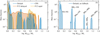 |
Fig. 14. Chirp-mass distributions of NS–NS, BH–NS, and BH–BH mergers for our default, the CPS, and the two F12 models (panel a), and for the default model without fallback (panel b). |
Also, the contribution from low-mass NSs from ECSNe of 1.25 M⊙ is visible by the double peak in the chirp-mass distribution of the NS–NS mergers and the shoulders towards lower chirp masses of the two BH + NS contributions. Accounting for fallback in the default model (Fig. 14a), we see that further components are added to the chirp-mass distribution. Assuming an average fallback BH mass of about 6 M⊙ (BHF) adds four components at logMchirp ≈ 0.38 (BHF + NS), logMchirp ≈ 0.70 (BHF + BHF), logMchirp ≈ 0.80 (BHF + BHL), and logMchirp ≈ 0.93 (BHF + BHH). Overall this leads to a smearing out of the main features.
Comparing the CPS model to the default model, we see that some features are shifted to lower chirp masses. For example, this is because the compactness peak is at lower CO core masses in single stars, and so the BH masses from stars in the compactness peak of the CPS model are lower than the corresponding masses in the default model (cf. Fig. B.1). All components in the chirp-mass distribution that involve BHL are thus slightly shifted to lower masses. The F12 rapid model also shows clearly separated contributions, but with more weight on BH–BH mergers compared to the other models, in particular the default and CPS models. The BH masses span a larger mass range in the F12 rapid model than in the default and CPS models, which leads to less substructured and broader BH–NS and BH–BH components in the chirp mass distribution. The most dramatic difference in the chirp-mass distribution is found in the F12 delayed model. In this model, there is no mass gap between NSs and BHs, and so there are no longer individual components in the NS–BH mass distribution and therefore none in the chirp-mass distribution either.
Our toy populations are only for stars of one metallicity and we have not incorporated the cosmic star-formation history. The chirp-mass distribution that will be available from gravitational-wave observations is going to be a convolution of various populations of different metallicities. As discussed in Sect. 4.1, the BH masses in particular depend for example on the total (wind) mass loss of stars. Stronger (weaker) winds at higher (lower) metallicities tend to shift BH masses to lower (higher) values. This way, we expect the components in the chirp-mass distribution to be effectively further smeared out in real observations.
6. Discussion
6.1. General remarks and uncertainties
Wind mass-loss rates of massive stars are uncertain (e.g. Smith 2014). This is true for winds of main sequence, (red) supergiant, and WR stars, and such uncertainties directly translate to various stellar properties up to core collapse (e.g. Renzo et al. 2017). The latter mass-loss rates are of particular relevance for stripped stars that become WR stars (e.g. Fryer et al. 2002), and extrapolating wind mass-loss rates from classical WR stars to lower mass helium stars after binary envelope stripping is problematic (Vink 2017; Gilkis et al. 2019). Stronger winds have the tendency to not only reduce the overall stellar masses but also core masses. Similarly to the most extreme form of mass loss, namely binary envelope stripping, the more mass lost by winds, the larger the core carbon mass fraction at core helium depletion, with similar consequences as discussed in this work for Case A and B stripped stars. Enhanced wind mass loss after core helium burning will most likely not drastically affect the pre-SN structure, analogously to what is found in Case C envelope stripping. While the final fate (e.g. explodability, compact remnant mass, explosion energy, etc.) is a non-monotonic function of the CO core mass, the general expectation is that stronger winds make it easier for stars to explode, enhance the NS formation rate, and lead to more energetic explosions, faster kicks, and higher nickel yields, and vice versa for weaker winds. Stellar winds scale with metallicity (cf. Sect. 2.1), such that stars at higher metallicity than those studied here experience more mass loss with the above-described consequences (and vice versa for stars at lower metallicity, hence weaker winds).
LBV-like mass loss via steady winds and eruptive episodes is not considered here, but will contribute to the total mass loss of stars. As discussed in Sect. 4.2.1 and shown in Fig. 7, this is most relevant for single stars that may produce BHs. Stripped binary stars only cross the LBV instability strip in the HR diagram before envelope removal and usually do not reach this regime thereafter. The enhanced mass loss through LBV-like winds will reduce the final total mass of stars and hence the BH mass. The BH masses from single stars reported in this work are therefore rather upper limits (cf. Fig. 7).
In this study, we have assumed that BHs form by direct collapse, that is, without neutrino emission. However, if BH-forming progenitors first form a proto-NS that then subsequently collapses to a BH, neutrinos can radiate away a non-negligible amount of energy and hence mass (≈0.3 M⊙) such that the outer layers of a star might get unbound and power a weak transient (Nadezhin 1980; Lovegrove & Woosley 2013; Coughlin et al. 2018). This in turn effectively reduces the BH mass. Because of this, it is often assumed that the resulting BH mass is 90% of the final baryonic mass of a star (e.g. Fryer et al. 2012). If most BHs do not form by direct collapse, our BH masses may be overestimated by about 10%. This most likely applies to the BHs formed by fallback in our models.
Convective (core) overshooting, or, more generally speaking, convective boundary mixing, greatly affects stars and remains an active field of research (e.g. Kippenhahn et al. 2012; Stancliffe et al. 2015). Convective core overshooting driven by the major burning cycles enlarges core masses and prolongs the respective burning cycle. For example, on the main sequence and during core helium burning, this implies that overshooting sets the relation between initial and CO/iron core mass, and therefore for example the relative numbers of NSs and BHs formed by a stellar population. More directly, a larger core overshooting on the main sequence allows stars to evolve to cooler temperatures, which has further implicit consequences: cooler stars lose more mass via winds and the total mass loss then affects the core evolution and hence final fate. We include moderate “step overshooting” of 0.2 pressure scale heights for core hydrogen and helium burning. A similar amount of overshooting is applied in some state-of-the-art stellar grids (e.g. Ekström et al. 2012; Chen et al. 2015), whereas in others an even larger overshooting is applied to match the wide main sequence at masses ≳10 − 15 M⊙ (e.g. Brott et al. 2011; Castro et al. 2014; Choi et al. 2016). Also, during the late burning stages, convective boundary mixing in shell-burning regions may trigger shell mergers, which could result in enhanced nuclear burning with consequences for the stellar structure. We do not consider convective boundary mixing beyond core helium burning.
The 12C(α, γ)16O reaction is key to several stellar astrophysical applications, but remains uncertain (e.g. deBoer et al. 2017). In Sect. 3.2, we stress the importance of the central carbon abundance after core helium burning for the evolution of stars towards core collapse. The 12C(α, γ)16O is key as it sets the rate at which carbon is converted into oxygen during the later phases of helium burning and thus sets the carbon abundance after this burning episode. Moreover, depending on the strength of this rate, the energy release and hence size of the convective core during helium burning could even be larger or smaller. As shown by Imbriani et al. (2001) for example, the exact 12C(α, γ)16O rate may influence whether core carbon burning proceeds convectively or radiatively with all the consequences for the pre-SN structure and SN as also discussed here. For example, the CO core mass range corresponding to the compactness peak and hence a possible island of BH formation is intimately connected to this reaction rate (see also Sukhbold & Adams 2020). However, regardless of the value of this rate, Case A and B stripped binary stars will always give rise to stars with a systematically larger carbon abundance after core helium burning than single and Case C stripped stars (Fig. 2).
Our models employ the approximate approx21_cr60_plus_co56.net nuclear reaction network in MESA. Such approximate networks are limited in their ability to accurately obtain the electron fraction Ye after oxygen burning. Larger networks are therefore required to more accurately follow the neutronisation and subsequent core collapse upon approaching the finite-temperature, effective Chandrasekhar mass (e.g. Weaver et al. 1978; Sukhbold et al. 2016; Farmer et al. 2016; Sukhbold et al. 2018). For example, Sukhbold et al. (2018) find variations in the central electron fraction at core collapse of Ye = 0.433 − 0.438 and Ye = 0.438 − 0.444 in an intially 15 M⊙ and 25 M⊙ star when switching from the “workhorse” network of 19 isotopes to a large network with about 300 isotopes that is fully coupled to the solver of the stellar structure equations. For the same initial masses, Farmer et al. (2016) report variations of Ye ≈ 0.415 − 0.425 and Ye ≈ 0.438 − 0.440, respectively, in their Fig. 21. In the Sukhbold et al. models, these variations correspond to final compactness values of ξ2.5 = 0.139 − 0.187 and ξ2.5 = 0.240 − 0.311 for the 15 M⊙ and 25 M⊙ stars, respectively. While such variations are non-negligible and add to the overall uncertainty on the final pre-SN structures of massive stars, here we are more interested in the systematic differences between genuine single and stripped binary stars.
As studied extensively by Farmer et al. (2016), the numerical meshing also affects pre-SN structures, and time-stepping and other numerical solver choices will do so too (e.g. we use varcontrol_target = 1d-4). For physical convergence, Farmer et al. (2016) recommend the use of zones no bigger than 0.01 M⊙ in MESA. While the absolute zoning is clearly important, adaptive mesh refinement and relative zoning are also crucial. To this end, the spatial zoning in our models is limited to relative cell masses of at most 10−3 (max_dq = 1d-3) and cells can be smaller (e.g. mesh_delta_coeff = 0.6 in our models).
6.2. Comparison to other stellar-evolution models
Several groups have computed pre-SN stellar models (e.g. to mention Woosley et al. 2002; Hirschi et al. 2004; Woosley & Heger 2007; Chieffi & Limongi 2013; Sukhbold & Woosley 2014; Sukhbold et al. 2016; Farmer et al. 2016; Sukhbold et al. 2018; Chieffi & Limongi 2020, a few more recent publications). All of these models have a shared commonality in that they predict a steep increase in the core compactness at the transition from convective to radiative core carbon burning. This transition and compactness peak is at different masses in the models because of different physics assumptions. For example, convective core overshooting, the still uncertain 12C(α, γ)16O nuclear reaction rate, and wind mass loss all affect the location of the compactness peak (see also Brown et al. 2001; Sukhbold & Adams 2020).
Furthermore, the compactness is observed to increase again beyond the compactness peak in many models, but this increase is closely connected to the adopted wind mass-loss routines, in particular the WR mass-loss rates (e.g. Woosley et al. 1993; Fryer et al. 2002). Larger wind mass loss (and in the most extreme case envelope stripping in binaries) are seen to reduce the compactness (see also Sukhbold et al. 2018), just as is found in this work. A systematic study looking into the evolution of pure CO cores with different initial carbon abundances towards core collapse (Patton & Sukhbold 2020) recovers this general landscape of compactness (or alternatively central entropy or iron core mass; cf. Sect. 3.2), and therefore this appears to be robust across different codes and assumptions on key physical processes.
Binary envelope stripping is often mimicked by considering helium star evolution (e.g. Woosley et al. 1995; McClelland & Eldridge 2016; Woosley 2019), but full binary evolution models up to core collapse are also available (e.g. Wellstein & Langer 1999; Fryer et al. 2002). From the evolution of stars without a hydrogen-rich envelope, Timmes et al. (1996) and Brown et al. (2001) found that stripped stars have a different pre-SN core structure and that this is related to the higher carbon mass fraction in stripped stars compared to single stars (see also Podsiadlowski et al. 2004, and Sect. 3.2). As we show in this work, these genuinely different core structures of stripped stars lead to a compactness peak shifted to higher CO core masses and a compactness that increases only at higher CO core masses in stripped stars compared to single stars (Fig. 5). This is in line with for example the findings of Woosley (2019) from helium star models (see also Ertl et al. 2020).
Our results further suggest that Case C envelope removal, that is, envelope stripping after core helium burning (Fig. 1), leads to similar compactness values as in single stars (e.g. the compactness peak is at the same CO core mass; Fig. 5). This is because the core structure in terms of CO core mass and core carbon mass fraction is already set at the end of core helium burning. However, we find that the explosion energies, kick velocities, and also compact remnant masses of Case C binary models are not necessarily the same as in single stars. For example, the binding energy of the envelope will be different as is the helium core mass. Helium star models are thus less suitable to describing Case C envelope removal.
6.3. Formation of NSs and BHs
The transition from NS to BH formation is sometimes thought to occur at a critical initial mass (see e.g. the well-known schematic picture in Heger et al. 2003). Such a simple picture is not supported by more recent studies, and a more complex, non-monotonic pattern of NS and BH formation has emerged (e.g. Sukhbold et al. 2016; Ertl et al. 2016). Whether or not these patterns are stochastic in nature has been discussed (Clausen et al. 2015).
Here, we find a somewhat less random landscape of NS and BH formation that closely follows the final compactness (or alternatively iron core mass or central entropy; see Sect. 3.2). Regardless of whether the pre-SN star is a genuine single star or has been stripped of its envelope by binary mass exchange, all models give rise to a compactness peak related to the transition from convective to radiative core carbon burning for which BH formation is found in our models. Beyond the compactness peak, NS formation is possible again, but we also find failed SN explosions and BH formation by fallback in cases where an explosion is triggered initially but stalls later on. In even more massive stars, a SN explosion is not found and BHs are formed (Fig. 7).
Observationally, BH rather than NS formation may manifest itself in the highly debated missing RSG problem, that is, in possibly missing high-luminosity stars (log L/L⊙ ≳ 5.1) among observed progenitors of Type IIP SNe (e.g. Smartt 2009, 2015). This luminosity threshold contrasts with the inferred maximum luminosity of RSGs of log L/L⊙ ≈ 5.5 in the Milky Way, and Small and Large Magellanic Clouds (Davies et al. 2018). Therefore, RSGs with log L/L⊙ ≈ 5.1 − 5.5 may not explode, but rather collapse to a BH. It should be noted that obtaining robust bolometric luminosities from pre-explosion photometry is challenging (e.g. Davies & Beasor 2018) and the maximum luminosity of SN IIP progenitors may be higher by 0.1 − 0.2 dex (e.g. Davies & Beasor 2020). Still, the missing RSG problem appears to persist at the 1 − 2σ significance level (Davies & Beasor 2020).
By monitoring a million supergiants for failed SNe (Kochanek et al. 2008), a first RSG of log L/L⊙ ≈ 5.3 − 5.5 was found to disappear without a SN IIP explosion (N6946-BH1; Gerke et al. 2015; Adams et al. 2017; Basinger et al. 2020). Instead, the star gave rise to a weak transient similar to the failed SN models of a star collapsing to a BH by Lovegrove & Woosley (2013).
Taken together, it seems that some RSGs collapse to a BH. Our single-star models in the compactness peak (Mini ≈ 21.5 − 23.5 M⊙) reach luminosities of log L/L⊙ ≈ 5.3 − 5.5 at core collapse and are predicted to form BHs (our stripped envelope models will give rise to SN Ib/c). This association of BH formation and the high compactness in RSGs that burn carbon radiatively in their core has also been made by Sukhbold & Adams (2020). These latter authors also find that the 12C(α, γ)16O reaction rate leads to significant uncertainty regarding the question of which RSG collapse to a BH (see discussion above).
Our single-star models predict NS formation for stars beyond the compactness peak such that it is conceivable that somewhat more luminous RSGs (log L/L⊙ ≳ 5.4 − 5.5 in our single-star models) explode again in Type IIP SNe and produce NSs. However, stellar winds in these stars are strong (see also Sect. 6.1) and the associated SN explosion might transition to Type II-L, II-b, or even I-b, depending on the remaining hydrogen-rich envelope.
The initial mass range for NS formation is considerably larger in our stripped binary models than in the single stars (Table 1). This has important ramifications for the occurrence of NSs and BHs in young star clusters and in massive binaries for example. Understanding the existence of the X-ray pulsar CXO J164710.2-455216 in the young star cluster Westerlund 1 with a turnoff mass of about 40 M⊙ is difficult if not impossible from a single-star point of view (Muno et al. 2006), because single stars of initially > 40 M⊙ are expected to form BHs. This implies that the progenitor star of CXO J164710.2-455216 experienced strong mass loss, for example via binary envelope stripping or an LBV-like (giant) eruption (see also Belczynski & Taam 2008, for a binary-stripping interpretation).
Similarly, the high present-day masses of companions to NSs in some X-ray binaries may only be understood when accounting for the binary-mass stripping history of the NS progenitors. However, this depends on how conservative mass transfer was in the evolution leading to the X-ray binary. For example, in the X-ray binary Wray 977/GX 301-2 (4U 1223-62), the B hypergiant companion Wray 977 has a current day inferred mass of 39 − 53 M⊙ (Kaper et al. 2006), that is, the total initial mass of the binary must have been larger than that. Within a non-conservative mass-transfer scenario, Ergma & van den Heuvel (1998) suggest an initial progenitor mass of > 50 M⊙ for the X-ray pulsar GX 301-2, while Wellstein & Langer (1999) show that within a more conservative mass-transfer scenario an initial progenitor mass of 26 M⊙ is sufficient to explain the present-day configuration of Wray 977. In both scenarios, our stripped binary models indeed predict NS formation.
6.4. NS–BH mass gap and X-ray binaries
Depending on the amount of fallback, our models do or do not show a mass gap between NSs and BHs (Sect. 4.2 and Fig. 9). Without fallback, the gap is at ≈2 − 9 M⊙ in the stripped binary stars and it narrows down to ≈2 − 5 M⊙ in the 50% fallback models. For smaller fallback fractions, the gap narrows down further. Therefore, the extent and existence of the gap is set by the SN physics. Only for sufficiently higher total mass loss than assumed here would models predict pre-SN stellar masses that could lead to a rather smooth transition from NSs to BHs without a gap (see also Fryer et al. 2002). This could be realised in stars at a metallicity significantly higher than solar.
Models of neutrino-driven explosions coupled to stellar models are in agreement with our conclusions on a possible NS–BH mass gap (Ugliano et al. 2012; Pejcha & Thompson 2015; Sukhbold et al. 2016, 2018; Müller et al. 2016). Other explosion models do not predict such a gap (e.g. Fryer & Kalogera 2001; Zhang et al. 2008; Fryer et al. 2012), but this depends on the assumption of whether an explosion is triggered rapidly or delayed. In the latter case (cf. F12 delayed model in Fig. 14), accretion of fallback material on the central compact remnant closes the NS–BH mass gap that is predicted in the rapid explosion model. As before, we therefore conclude that fallback or accretion onto a central compact object in delayed SN explosions is the main mechanism that governs the existence and width of a possible NS–BH mass gap (see also Belczynski et al. 2012; Kochanek 2014; Chan et al. 2020).
From observations of Galactic X-ray binaries, Özel et al. (2010) and Farr et al. (2011) infer BH masses of ≳5 M⊙ (see also Casares et al. 2017). Together with a maximum NS mass of about 2 M⊙ (e.g. Demorest et al. 2010; Antoniadis et al. 2013), this suggested a NS–BH mass gap in the range 2 − 5 M⊙. Kreidberg et al. (2012) caution that systematic errors could have lead to overestimated BH masses from some X-ray binaries, which may reduce the determined BH masses to a value inside the mass gap.
The existence of this gap is challenged. First, Thompson et al. (2019) report the discovery of a ≈83 d binary containing a rapidly rotating giant star and a  dark object, most likely a BH. Secondly, there are claims with potentially large systematic uncertainties of pulsars with masses above 2 M⊙, such as for example the ≈2.7 M⊙ millisecond pulsar in the globular cluster NGC 6440 (Freire et al. 2008). Thirdly, in gravitational microlensing events, compact objects in the NS–BH mass gap may have been found (Wyrzykowski & Mandel 2020). The individual mass measurements of these objects are consistent with masses ≲2 M⊙ and ≳5 M⊙ within their uncertainties. However, interpreting all individual observations simultaneously within a certain model for the compact-object mass distribution, Wyrzykowski & Mandel (2020) strongly disfavour the existence of a NS–BH mass gap at 2 − 5 M⊙. Finally, from gravitational-wave emission of merging compact objects, Abbott et al. (2020b) report the merger of a 22.2 − 24.3 M⊙ BH with a 2.50 − 2.67 M⊙ compact companion (GW190814; 90% credibility intervals). Previously, only BHs of masses of ≳7 M⊙ had been observed in gravitational-wave merger events (e.g. Abbott et al. 2019). The previous BH–BH mergers did not invoke BHs of such unequal masses, which may point to a rarer formation channel. It therefore seems that the previous suggestion of the existence of a NS–BH mass gap may no longer hold true.
In principle, compact objects in X-ray binaries can trace intrinsically different compact-object populations, and may have different evolutionary paths and even different origins from compact objects observed in wide binaries without detectable X-ray emission, found in microlensing surveys, and detected as gravitational-wave merger events. For example, microlensing can find the remnants of NS–NS mergers (e.g. the 2.7 M⊙ remnant of GW170817; Abbott et al. 2017), primordial BHs (e.g. Zel’dovich & Novikov 1967; Hawking 1971; Carr et al. 2016), and also BHs ejected from binary systems by SN kicks (e.g. Willems et al. 2005; Fragos et al. 2009). Similarly, the unusually large mass ratio of GW190814 may point to a rare formation channel (Abbott et al. 2020b).
If BHs form via direct collapse, they might not receive a kick. In our fallback cases, as discussed in Sect. 4.4, BHs receive a kick and the kick velocity is larger for smaller amounts of fallback material. This means that the least massive BHs that formed via fallback receive the largest kicks and the most massive BHs receive the smallest kicks. In our models, BHs ≲9 M⊙ in stripped binary stars (and ≲12 M⊙ in single stars) receive kicks whereas more massive BHs might not. From our toy population model we see that about 50–60% of BHs are single and no longer in binaries. Within our models, the formation of BHs with the least fallback is most likely to break up binaries by SN kicks and this population of low-mass BHs may explain some of the NS–BH mass gap objects found by Wyrzykowski & Mandel (2020). This idea does not exclude the existence of BHs of 2 − 5 M⊙ in X-ray binaries, but it would make it less likely and could help to reduce some of the apparent tension.
From observations of X-ray binaries, it is clear that some BHs formed in a SN and received a kick, because the companion stars show chemical signatures of a SN event and the binary has a high space velocity (see e.g. GRO J1655-40, also known as Nova Sco 1994; Brandt et al. 1995; Israelian et al. 1999; Podsiadlowski et al. 2002; Willems et al. 2005). Also, the large distance to the plane of the Milky Way of BH X-ray binaries suggests that they have received a kick (e.g. Jonker & Nelemans 2004; Repetto & Nelemans 2015). As noted by Casares et al. (2017), it is interesting that Cygnus X-1 and GRS 1915+105, X-ray binaries with BHs of ≈15 M⊙ and ≈12 M⊙, respectively, likely received no or only a small kick (e.g. Mirabel & Rodrigues 2003; Reid et al. 2014), whereas XTE J1118+480 (e.g. Mirabel et al. 2001; Fragos et al. 2009), the aforementioned GRO J1655-40, and likely also V404 Cygni (e.g. Miller-Jones et al. 2009a,b) with BH masses of ≈7 − 8 M⊙, ≈5.4 M⊙, and ≈9 M⊙, respectively, probably formed with a natal kick. This could indeed be a hint that less massive BHs are formed with a higher kick than their more massive counterparts.
The most massive BH in our stripped binary models is ≈20 M⊙, which is somewhat larger than one of the most massive BHs observed in an X-ray binary in the Milky Way (i.e. Cyg X-1 with ≈15 M⊙, Orosz et al. 2011). As discussed in Sect. 6.1, if BHs do not form by direct collapse, but if a proto-NS is formed first that can emit neutrinos, our BH masses are somewhat overestimated. In general, the most massive BH in stripped stars is closely linked to the WR wind mass loss after the loss of the hydrogen-rich envelope (see also Fryer et al. 2002). Therefore, while the difference between our maximum BH mass and that of Cyg X-1 is not large, it may suggest that the WR wind mass loss applied in our models is too low.
Starting from the observed WR + OB binary stars in the Galaxy, Vanbeveren et al. (2020) predict the expected population of wind-fed BH high-mass X-ray binaries. Under the assumption that the WR stars collapse to BHs with kicks insufficient to break up the WR + OB binaries, these latter authors expect to find more than 100 such BH X-ray binaries whereas only one (Cyg X-1) is observed. Given this stark discrepancy, Vanbeveren et al. (2020) conclude that the WR stars either formed BHs that received a significant kick or that they collapsed to NSs. Most of the Galactic WR + OB binaries considered in Vanbeveren et al. (2020) have such short orbital periods that they must have undergone a past mass-transfer episode in which the current WR star lost its envelope to its companion star. From our models, we therefore expect that most of these stripped WR stars will form a NS at the end of their life, thereby offering a natural solution to this discrepancy.
6.5. Explosion energies, nickel yields, and kicks
Observations of SN light curves suggest that, on average, stripped-envelope SNe produce more 56 Ni and are more energetic than SN IIP (e.g. Anderson 2019; Meza & Anderson 2020; Sharon & Kushnir 2020; Afsariardchi et al. 2020), exactly as predicted by our models (Sect. 4.3). At first glance, the observed differences are quite dramatic; for example, the recent meta-analysis of Anderson (2019) gives median values of 0.032 M⊙ for the nickel mass MNi for Type II SNe and 0.16 M⊙ for Type Ib/c SNe (excluding broad-lined Type Ic events). Closer inspection suggests less dramatic differences, that is, when taking into account selection effects and systematic uncertainties in determining MNi.
For Type IIP SNe, Müller et al. (2017) recently determined the distribution of nickel masses quite reliably from the tail phase based on a sample whose representative character was established by comparison with the LOSS survey (Li et al. 2011), finding a median of 0.031 M⊙ and a mean of 0.046 M⊙. For stripped-envelope SNe, the distribution of explosion properties is less securely established. Although a number of studies have investigated light-curve parameters and/or explosion properties for larger samples of stripped-envelope SNe (e.g. Drout et al. 2011; Bianco et al. 2014; Lyman et al. 2016; Prentice et al. 2016, 2019; Taddia et al. 2018), these are usually not based on volume-limited surveys (for an exception, see Li et al. 2011), and nickel masses are often inferred from the peak luminosity using Arnett’s rule (Arnett 1982).
Although the precise impact of selection biases for transients is not straightforward to determine, the classical formula for the Malmquist bias provides a rough estimate. Based on a standard deviation of 0.71 − 0.78 mag in peak luminosity in the SN Ib/c sample of Prentice et al. (2016), the average peak luminosity may be overestimated by about 0.7 − 0.8 mag in samples that are not volume limited, which translates into a factor of two in nickel mass. The differences between the volume-limited sample of Li et al. (2011) and other population studies of stripped-envelope explosions are indeed of similar magnitude. Arnett’s rule also tends to systematically overestimate nickel masses in Ib/c SNe by about 50% (Dessart et al. 2015). It is therefore likely that the average nickel mass in stripped-envelope explosions (excluding broad-lined Ic SNe) is only ∼70% higher than for Type IIP and not by a factor of five as suggested by Anderson (2019).
Our models indicate that modestly higher nickel masses (about 50%) in stripped-envelope explosions might be explained naturally as a consequence of binary mass transfer and its impact on the subsequent stages of stellar evolution. After accounting for biases in observationally inferred nickel masses, there may be no pressing need to invoke magnetar powering for a substantial fraction of stripped-envelope SNe as advocated by Ertl et al. (2020). Observed outliers among Ib/c SNe with high peak luminosity and nickel masses ≳0.20 − 0.25 (Fig. 11c) still cannot be directly explained by our sample of stripped-envelope progenitors. However, viewing angle effects could partly account for such events; moderate asymmetries in the nickel distribution may well increase the peak luminosity and the “apparent” nickel mass by about 0.5 mag or 60% (Sim et al. 2007).
The calibration of our kick velocities includes single and stripped stars and is made with respect to the observed space velocities of pulsars as found by Hobbs et al. (2005), that is, to a Maxwellian distribution with σ = 265 km s−1. Here, we find that stripped stars receive an intrinsically larger kick (σ = 315 ± 24 km s−1) than single stars (σ = 222 ± 23 km s−1). While these σ values are not dramatically different from the Hobbs et al. (2005) distribution (about ±15 − 20%), they are relevant for example for interpretation of the observed space velocities of X-ray and other compact-object binaries; they would also reduce rate predictions of compact-object mergers from isolated binaries and slightly increase expectations for space velocities of runaway and walkaway stars (see e.g. Renzo et al. 2019).
As stressed in Sect. 2.3, we only consider mean kick velocities and not also the dispersions that are inherent to stochastic kick formation. While the diversity of our pre-SN models gives rise to a distribution of mean kick velocities that appears to be generally compatible with observations of for example Hobbs et al. (2005), the stochastic nature of kicks will further affect the shape of the distribution such that a more in-depth comparison to observations cannot be made at this point.
7. Conclusions
Most massive stars reside in binary systems such that they will exchange mass with their companions at some point during their lives. Here, we study how Case A, B, and C envelope stripping affects the further evolution of stars up to core collapse and thereby their explosion properties. The stars were modelled using the MESA stellar evolution code and the SN stage were analysed with the parametric SN model of Müller et al. (2016). Our main results can be summarised as follows.
-
Because of the removal of the hydrogen-rich envelope, Case A and B stripped stars have larger core carbon abundances XC after core helium burning than single and Case C stripped stars for the same CO core masses MCO; the Case A and B stripped stars form a distinct branch in the MCO–XC plane (Fig. 2).
-
The two key quantities MCO and XC largely determine the core evolution through the advanced nuclear burning phases up to core collapse. Because of the distinct differences of stripped and single stars, we find different pre-SN structures in these stars. For example, the Case A and B stripped stars have on average lower iron core masses for the same MCO compared to single and Case C stripped stars, and the compactness parameter ξ2.5 is also different. Both single and stripped stars show a compactness peak at certain MCO values related to the transition from convective to radiative core carbon burning. In both cases, there is also a steep increase in ξ2.5 beyond some MCO. Importantly, the compactness peak and steep increase in compactness are at higher MCO in Case A and B stripped stars than in single and Case C stripped stars.
-
The structural differences translate into differences in the SN properties. Compared to single stars, Case A and B stripped stars result in lower NS and BH masses (ΔMNS ≈ 0.05 M⊙), higher explosion energies (ΔEexpl ≈ 0.2 B), larger kicks (Δvkick ≈ 100 km s−1), and larger nickel yields (ΔMNi ≈ 0.02 M⊙) on average. Kick velocities of ≳600 km s−1 are almost exclusively found in stripped stars. Setting BHs from stars in the compactness peak aside, single and Case C stripped stars give rise to BHs for initial masses Mini ≳ 35 M⊙ while this limit shifts to Mini ≳ 70 M⊙ in Case A and B stripped stars.
-
Some models beyond the compactness peak likely experience significant fallback and probably a weak or failed SN. The BHs formed from envelope material falling back onto the NS receive a kick that is substantially lower than that of the original NS (depending on the amount of fallback).
-
The NS mass distribution is unimodal with a tail extending up to the maximum allowed NS mass of 2.0 M⊙; that is, some NSs are born massive (we do not consider the contributions from ECSNe and ultra-stripped stars). The BH mass distribution is multimodal: stars falling into the compactness peak give rise to an island of BH formation, and the lowest mass BHs are always from stripped stars. The maximum BH mass from our stripped envelope models is about 20 M⊙ (that of single stars is larger and depends on the amount of mass loss during LBV phases). There is a gap between NSs and BHs in our models if we discard fallback. The gap may (partly) disappear depending on the amount of fallback (low fallback fractions reduce the gap and high fallback fractions maximise it). The features in the compact remnant mass distributions give rise to distinct peaks in the chirp-mass distribution of NS–NS, BH–NS, and BH–BH mergers.
-
At least one star (if not both stars) in compact-object mergers from isolated binary evolution will have evolved through envelope stripping. Because the initial mass range for NS formation is largely enhanced in stripped stars, we find a significant reduction of BHs in stellar populations. For example, the NS-to-BH ratio is ≈15 in our Case B stripped models whereas it is only 2–3 for our stellar models when applying the delayed and rapid SN models of Fryer et al. (2012), which are frequently applied in state-of-the-art population-synthesis models. Consequently, the expected BH–NS and BH–BH merger rates are reduced, and from a simplified population-synthesis model we find reductions of 25–50% and 90%, respectively.
-
Relative to the Fryer et al. (2012) SN model, the NS–NS merger rate in our default population model increases only marginally (6–15%). This is because a large fraction of NS–NS mergers forms from low-kick SNe (e.g. ECSNe and stars with low iron cores) that are not affected by the increase in the initial-mass parameter space for NS formation from stripped stars.
We conclude that the removal of the hydrogen-rich envelope not only naturally affects the SN type (II vs. Ib/c), but has severe implications for the interior structure and evolution of stars, and thus the SN explosion itself. This will in turn help to further our understanding of NS and BH formation, the explosion properties of SNe, compact-object binaries, and gravitational-wave merger events.
Oxygen burning and beyond proceed under convective conditions.
Whether the convective-core size stays constant or decreases depends on the mass loss of a star during core helium burning. In massive stars with strong winds, the mass of the convective core decreases.
Switching-off WR winds would reduce the separation between the two branches in Fig. 2, and turning up these wind mass-loss rates would increase it.
This is less clear for NSs from Case C mass transfer, which rather scatter around the NS masses of single stars.
The best-fitting Maxwellian distributions are for σ = 218 ± 24 km s−1 and σ = 321 ± 27 km s−1 in the 50% fallback model.
More precisely, we do not necessarily only have ECSNe in mind, but also collapsing stars with very small iron cores that are not expected to produce large SN kicks (Podsiadlowski et al. 2004). Such stars are commonly produced in Case BB mass transfer and are referred to as ultra-stripped stars (Tauris et al. 2015). With this definition in mind, the initial mass range over which low SN kicks are found could even be larger than what we assume here.
Not shown in Fig. 13a.
This means that the intrinsic chirp-mass distribution can be obtained by dividing the shown distribution by  (see Sect. 5.3).
Acknowledgments
BM was supported by ARC Future Fellowship FT160100035. We thank the referee for carefully reading our manuscript and the useful comments that helped to improve it. Moreover, we thank Danny Vanbeveren for pointing out that NS formation for stripped stars of initially up to 70 M⊙ can explain why most of the observed WR + OB binaries may not produce wind-fed (BH) high-mass X-ray binaries and thereby helps to understand a discrepancy they reported in Vanbeveren et al. (2020). This research made use of NumPy (Oliphant 2006), SciPy (Virtanen et al. 2020), Matplotlib (Hunter 2007) and Jupyter Notebooks (Kluyver et al. 2016).
References
- Abate, C., Pols, O. R., Izzard, R. G., Mohamed, S. S., & de Mink, S. E. 2013, A&A, 552, A26 [NASA ADS] [CrossRef] [EDP Sciences] [Google Scholar]
- Abbott, B. P., Abbott, R., Abbott, T. D., et al. 2017, Phys. Rev. Lett., 119, 161101 [NASA ADS] [CrossRef] [PubMed] [Google Scholar]
- Abbott, B. P., Abbott, R., Abbott, T. D., et al. 2019, Phys. Rev. X, 9, 031040 [Google Scholar]
- Abbott, B. P., Abbott, R., Abbott, T. D., et al. 2020a, ApJ, 892, L3 [Google Scholar]
- Abbott, R., Abbott, T. D., Abraham, S., et al. 2020b, ApJ, 896, L44 [Google Scholar]
- Adams, S. M., Kochanek, C. S., Gerke, J. R., Stanek, K. Z., & Dai, X. 2017, MNRAS, 468, 4968 [NASA ADS] [CrossRef] [Google Scholar]
- Afsariardchi, N., Drout, M. R., Khatami, D., et al. 2020, ApJ, submitted [Google Scholar]
- Anderson, J. P. 2019, A&A, 628, A7 [NASA ADS] [CrossRef] [EDP Sciences] [Google Scholar]
- Antoniadis, J., Freire, P. C. C., Wex, N., et al. 2013, Science, 340, 448 [Google Scholar]
- Arnett, W. D. 1982, ApJ, 253, 785 [NASA ADS] [CrossRef] [Google Scholar]
- Asplund, M., Grevesse, N., Sauval, A. J., & Scott, P. 2009, ARA&A, 47, 481 [NASA ADS] [CrossRef] [Google Scholar]
- Banerjee, S. 2017, MNRAS, 467, 524 [NASA ADS] [Google Scholar]
- Basinger, C. M., Kochanek, C. S., Adams, S. M., Dai, X., & Stanek, K. Z. 2020, ArXiv e-prints [arXiv:2007.15658] [Google Scholar]
- Belczynski, K., & Taam, R. E. 2008, ApJ, 685, 400 [NASA ADS] [CrossRef] [Google Scholar]
- Belczynski, K., Kalogera, V., & Bulik, T. 2002, ApJ, 572, 407 [NASA ADS] [CrossRef] [Google Scholar]
- Belczynski, K., Wiktorowicz, G., Fryer, C. L., Holz, D. E., & Kalogera, V. 2012, ApJ, 757, 91 [NASA ADS] [CrossRef] [Google Scholar]
- Belczynski, K., Klencki, J., Fields, C. E., et al. 2020, A&A, 636, A104 [CrossRef] [EDP Sciences] [Google Scholar]
- Bethe, H. A., & Brown, G. E. 1998, ApJ, 506, 780 [NASA ADS] [CrossRef] [Google Scholar]
- Bianco, F. B., Modjaz, M., Hicken, M., et al. 2014, ApJS, 213, 19 [NASA ADS] [CrossRef] [Google Scholar]
- Brandt, W. N., Podsiadlowski, P., & Sigurdsson, S. 1995, MNRAS, 277, L35 [NASA ADS] [Google Scholar]
- Brott, I., de Mink, S. E., Cantiello, M., et al. 2011, A&A, 530, A115 [NASA ADS] [CrossRef] [EDP Sciences] [Google Scholar]
- Brown, G. E., Weingartner, J. C., & Wijers, R. A. M. J. 1996, ApJ, 463, 297 [NASA ADS] [CrossRef] [Google Scholar]
- Brown, G. E., Heger, A., Langer, N., et al. 2001, New Astron., 6, 457 [NASA ADS] [CrossRef] [Google Scholar]
- Burrows, A., Radice, D., Vartanyan, D., et al. 2020, MNRAS, 491, 2715 [CrossRef] [Google Scholar]
- Carr, B., Kühnel, F., & Sandstad, M. 2016, Phys. Rev. D, 94, 083504 [CrossRef] [Google Scholar]
- Casares, J., Jonker, P. G., & Israelian, G. 2017, in X-Ray Binaries, eds. A. W. Alsabti, & P. Murdin, 1499 [Google Scholar]
- Castro, N., Fossati, L., Langer, N., et al. 2014, A&A, 570, L13 [NASA ADS] [CrossRef] [EDP Sciences] [Google Scholar]
- Chabrier, G. 2003, PASP, 115, 763 [Google Scholar]
- Chan, C., Müller, B., & Heger, A. 2020, MNRAS, 495, 3751 [CrossRef] [Google Scholar]
- Chen, Y., Bressan, A., Girardi, L., et al. 2015, MNRAS, 452, 1068 [NASA ADS] [CrossRef] [Google Scholar]
- Chieffi, A., & Limongi, M. 2013, ApJ, 764, 21 [NASA ADS] [CrossRef] [Google Scholar]
- Chieffi, A., & Limongi, M. 2020, ApJ, 890, 43 [CrossRef] [Google Scholar]
- Chini, R., Hoffmeister, V. H., Nasseri, A., Stahl, O., & Zinnecker, H. 2012, MNRAS, 424, 1925 [Google Scholar]
- Choi, J., Dotter, A., Conroy, C., et al. 2016, ApJ, 823, 102 [Google Scholar]
- Clausen, D., Piro, A. L., & Ott, C. D. 2015, ApJ, 799, 190 [NASA ADS] [CrossRef] [Google Scholar]
- Coughlin, E. R., Quataert, E., Fernández, R., & Kasen, D. 2018, MNRAS, 477, 1225 [CrossRef] [Google Scholar]
- Cyburt, R. H., Amthor, A. M., Ferguson, R., et al. 2010, ApJS, 189, 240 [NASA ADS] [CrossRef] [Google Scholar]
- Davies, B., & Beasor, E. R. 2018, MNRAS, 474, 2116 [Google Scholar]
- Davies, B., & Beasor, E. R. 2020, MNRAS, 493, 468 [NASA ADS] [CrossRef] [Google Scholar]
- Davies, B., Crowther, P. A., & Beasor, E. R. 2018, MNRAS, 478, 3138 [NASA ADS] [CrossRef] [Google Scholar]
- De Marco, O., & Izzard, R. G. 2017, PASA, 34, e001 [NASA ADS] [CrossRef] [Google Scholar]
- deBoer, R. J., Görres, J., Wiescher, M., et al. 2017, Rev. Mod. Phys., 89, 035007 [NASA ADS] [CrossRef] [Google Scholar]
- Demorest, P. B., Pennucci, T., Ransom, S. M., Roberts, M. S. E., & Hessels, J. W. T. 2010, Nature, 467, 1081 [Google Scholar]
- Dessart, L., Hillier, D. J., Woosley, S., et al. 2015, MNRAS, 453, 2189 [NASA ADS] [CrossRef] [Google Scholar]
- Drout, M. R., Soderberg, A. M., Gal-Yam, A., et al. 2011, ApJ, 741, 97 [NASA ADS] [CrossRef] [Google Scholar]
- Ekström, S., Georgy, C., Eggenberger, P., et al. 2012, A&A, 537, A146 [NASA ADS] [CrossRef] [EDP Sciences] [Google Scholar]
- Eldridge, J. J., & Vink, J. S. 2006, A&A, 452, 295 [NASA ADS] [CrossRef] [EDP Sciences] [Google Scholar]
- Eldridge, J. J., & Stanway, E. R. 2016, MNRAS, 462, 3302 [NASA ADS] [CrossRef] [Google Scholar]
- Ergma, E., & van den Heuvel, E. P. J. 1998, A&A, 331, L29 [Google Scholar]
- Ertl, T., Janka, H.-T., Woosley, S. E., Sukhbold, T., & Ugliano, M. 2016, ApJ, 818, 124 [NASA ADS] [CrossRef] [Google Scholar]
- Ertl, T., Woosley, S. E., Sukhbold, T., & Janka, H. T. 2020, ApJ, 890, 51 [CrossRef] [Google Scholar]
- Farmer, R., Fields, C. E., Petermann, I., et al. 2016, ApJS, 227, 22 [NASA ADS] [CrossRef] [Google Scholar]
- Farr, W. M., Sravan, N., Cantrell, A., et al. 2011, ApJ, 741, 103 [NASA ADS] [CrossRef] [Google Scholar]
- Ferguson, J. W., Alexander, D. R., Allard, F., et al. 2005, ApJ, 623, 585 [NASA ADS] [CrossRef] [Google Scholar]
- Finn, L. S. 1996, Phys. Rev. D, 53, 2878 [NASA ADS] [CrossRef] [Google Scholar]
- Finn, L. S., & Chernoff, D. F. 1993, Phys. Rev. D, 47, 2198 [NASA ADS] [CrossRef] [Google Scholar]
- Fragos, T., Willems, B., Kalogera, V., et al. 2009, ApJ, 697, 1057 [NASA ADS] [CrossRef] [Google Scholar]
- Freire, P. C. C., Ransom, S. M., Bégin, S., et al. 2008, ApJ, 675, 670 [NASA ADS] [CrossRef] [Google Scholar]
- Fryer, C. L., & Kalogera, V. 2001, ApJ, 554, 548 [NASA ADS] [CrossRef] [Google Scholar]
- Fryer, C. L., Heger, A., Langer, N., & Wellstein, S. 2002, ApJ, 578, 335 [NASA ADS] [CrossRef] [Google Scholar]
- Fryer, C. L., Belczynski, K., Wiktorowicz, G., et al. 2012, ApJ, 749, 91 [NASA ADS] [CrossRef] [Google Scholar]
- Gerke, J. R., Kochanek, C. S., & Stanek, K. Z. 2015, MNRAS, 450, 3289 [NASA ADS] [CrossRef] [Google Scholar]
- Giacobbo, N., & Mapelli, M. 2018, MNRAS, 480, 2011 [NASA ADS] [CrossRef] [Google Scholar]
- Giacobbo, N., & Mapelli, M. 2020, ApJ, 891, 141 [CrossRef] [Google Scholar]
- Gilkis, A., Vink, J. S., Eldridge, J. J., & Tout, C. A. 2019, MNRAS, 486, 4451 [NASA ADS] [CrossRef] [Google Scholar]
- Götberg, Y., de Mink, S. E., & Groh, J. H. 2017, A&A, 608, A11 [NASA ADS] [CrossRef] [EDP Sciences] [Google Scholar]
- Hawking, S. 1971, MNRAS, 152, 75 [NASA ADS] [CrossRef] [Google Scholar]
- Heger, A., Fryer, C. L., Woosley, S. E., Langer, N., & Hartmann, D. H. 2003, ApJ, 591, 288 [NASA ADS] [CrossRef] [Google Scholar]
- Henyey, L., Vardya, M. S., & Bodenheimer, P. 1965, ApJ, 142, 841 [NASA ADS] [CrossRef] [Google Scholar]
- Hirschi, R., Meynet, G., & Maeder, A. 2004, A&A, 425, 649 [NASA ADS] [CrossRef] [EDP Sciences] [Google Scholar]
- Hobbs, G., Lorimer, D. R., Lyne, A. G., & Kramer, M. 2005, MNRAS, 360, 974 [NASA ADS] [CrossRef] [Google Scholar]
- Hunter, J. D. 2007, Comput. Sci. Eng., 9, 90 [NASA ADS] [CrossRef] [Google Scholar]
- Iglesias, C. A., & Rogers, F. J. 1996, ApJ, 464, 943 [NASA ADS] [CrossRef] [Google Scholar]
- Imbriani, G., Limongi, M., Gialanella, L., et al. 2001, ApJ, 558, 903 [NASA ADS] [CrossRef] [Google Scholar]
- Israelian, G., Rebolo, R., Basri, G., Casares, J., & Martín, E. L. 1999, Nature, 401, 142 [NASA ADS] [CrossRef] [Google Scholar]
- Janka, H.-T. 2017, ApJ, 837, 84 [NASA ADS] [CrossRef] [Google Scholar]
- Jonker, P. G., & Nelemans, G. 2004, MNRAS, 354, 355 [NASA ADS] [CrossRef] [Google Scholar]
- Kaper, L., van der Meer, A., & Najarro, F. 2006, A&A, 457, 595 [NASA ADS] [CrossRef] [EDP Sciences] [Google Scholar]
- Kasen, D., & Woosley, S. E. 2009, ApJ, 703, 2205 [NASA ADS] [CrossRef] [Google Scholar]
- Katsuda, S., Morii, M., Janka, H.-T., et al. 2018, ApJ, 856, 18 [NASA ADS] [CrossRef] [Google Scholar]
- Kippenhahn, R., & Weigert, A. 1967, ZAp, 65, 251 [Google Scholar]
- Kippenhahn, R., Weigert, A., & Weiss, A. 2012, Stellar Structure and Evolution [Google Scholar]
- Kluyver, T., Ragan-Kelley, B., Pérez, F., et al. 2016, in Positioning and Power in Academic Publishing: Players, Agents and Agendas, eds. F. Loizides, B. Schmidt, et al. (IOS Press), 87 [Google Scholar]
- Kobulnicky, H. A., & Fryer, C. L. 2007, ApJ, 670, 747 [NASA ADS] [CrossRef] [Google Scholar]
- Kobulnicky, H. A., Kiminki, D. C., Lundquist, M. J., et al. 2014, ApJS, 213, 34 [NASA ADS] [CrossRef] [Google Scholar]
- Kochanek, C. S. 2014, ApJ, 785, 28 [NASA ADS] [CrossRef] [Google Scholar]
- Kochanek, C. S., Beacom, J. F., Kistler, M. D., et al. 2008, ApJ, 684, 1336 [NASA ADS] [CrossRef] [Google Scholar]
- Kreidberg, L., Bailyn, C. D., Farr, W. M., & Kalogera, V. 2012, ApJ, 757, 36 [NASA ADS] [CrossRef] [Google Scholar]
- Kroupa, P. 2001, MNRAS, 322, 231 [NASA ADS] [CrossRef] [Google Scholar]
- Kruckow, M. U., Tauris, T. M., Langer, N., Kramer, M., & Izzard, R. G. 2018, MNRAS, 481, 1908 [NASA ADS] [CrossRef] [Google Scholar]
- Langer, N. 2012, ARA&A, 50, 107 [NASA ADS] [CrossRef] [Google Scholar]
- Langer, N., Schürmann, C., Stoll, K., et al. 2020, A&A, 638, A39 [CrossRef] [EDP Sciences] [Google Scholar]
- Laplace, E., Götberg, Y., de Mink, S. E., Justham, S., & Farmer, R. 2020, A&A, 637, A6 [CrossRef] [EDP Sciences] [Google Scholar]
- Lattimer, J. M., & Yahil, A. 1989, ApJ, 340, 426 [NASA ADS] [CrossRef] [Google Scholar]
- Lattimer, J. M., & Prakash, M. 2001, ApJ, 550, 426 [NASA ADS] [CrossRef] [Google Scholar]
- Li, W., Leaman, J., Chornock, R., et al. 2011, MNRAS, 412, 1441 [NASA ADS] [CrossRef] [Google Scholar]
- Lin, J., Rappaport, S., Podsiadlowski, P., et al. 2011, ApJ, 732, 70 [NASA ADS] [CrossRef] [Google Scholar]
- Lovegrove, E., & Woosley, S. E. 2013, ApJ, 769, 109 [NASA ADS] [CrossRef] [Google Scholar]
- Lyman, J. D., Bersier, D., James, P. A., et al. 2016, MNRAS, 457, 328 [NASA ADS] [CrossRef] [Google Scholar]
- Mandel, I., & de Mink, S. E. 2016, MNRAS, 458, 2634 [NASA ADS] [CrossRef] [Google Scholar]
- Mapelli, M. 2016, MNRAS, 459, 3432 [NASA ADS] [CrossRef] [Google Scholar]
- Marchant, P., Langer, N., Podsiadlowski, P., Tauris, T. M., & Moriya, T. J. 2016, A&A, 588, A50 [NASA ADS] [CrossRef] [EDP Sciences] [Google Scholar]
- Mason, B. D., Hartkopf, W. I., Gies, D. R., Henry, T. J., & Helsel, J. W. 2009, AJ, 137, 3358 [NASA ADS] [CrossRef] [EDP Sciences] [Google Scholar]
- Mauron, N., & Josselin, E. 2011, A&A, 526, A156 [NASA ADS] [CrossRef] [EDP Sciences] [Google Scholar]
- McClelland, L. A. S., & Eldridge, J. J. 2016, MNRAS, 459, 1505 [NASA ADS] [CrossRef] [Google Scholar]
- Mennekens, N., & Vanbeveren, D. 2014, A&A, 564, A134 [NASA ADS] [CrossRef] [EDP Sciences] [Google Scholar]
- Meza, N., & Anderson, J. P. 2020, A&A, 641, A177 [CrossRef] [EDP Sciences] [Google Scholar]
- Miller-Jones, J. C. A., Jonker, P. G., Dhawan, V., et al. 2009a, ApJ, 706, L230 [NASA ADS] [CrossRef] [Google Scholar]
- Miller-Jones, J. C. A., Jonker, P. G., Nelemans, G., et al. 2009b, MNRAS, 394, 1440 [NASA ADS] [CrossRef] [Google Scholar]
- Mirabel, I. F., & Rodrigues, I. 2003, Science, 300, 1119 [NASA ADS] [CrossRef] [PubMed] [Google Scholar]
- Mirabel, I. F., Dhawan, V., Mignani, R. P., Rodrigues, I., & Guglielmetti, F. 2001, Nature, 413, 139 [NASA ADS] [CrossRef] [PubMed] [Google Scholar]
- Moe, M., & Di Stefano, R. 2017, ApJS, 230, 15 [Google Scholar]
- Mohamed, S., & Podsiadlowski, P. 2007, in 15th European Workshop on White Dwarfs, eds. R. Napiwotzki, & M. R. Burleigh, ASP Conf. Ser., 372, 397 [Google Scholar]
- Müller, B., Heger, A., Liptai, D., & Cameron, J. B. 2016, MNRAS, 460, 742 [NASA ADS] [CrossRef] [Google Scholar]
- Müller, T., Prieto, J. L., Pejcha, O., & Clocchiatti, A. 2017, ApJ, 841, 127 [NASA ADS] [CrossRef] [Google Scholar]
- Müller, B., Tauris, T. M., Heger, A., et al. 2019, MNRAS, 484, 3307 [CrossRef] [Google Scholar]
- Muno, M. P., Clark, J. S., Crowther, P. A., et al. 2006, ApJ, 636, L41 [NASA ADS] [CrossRef] [Google Scholar]
- Nadezhin, D. K. 1980, Ap&SS, 69, 115 [NASA ADS] [CrossRef] [Google Scholar]
- Nakamura, K., Takiwaki, T., Kuroda, T., & Kotake, K. 2015, PASJ, 67, 107 [NASA ADS] [CrossRef] [Google Scholar]
- Nieuwenhuijzen, H., & de Jager, C. 1990, A&A, 231, 134 [NASA ADS] [Google Scholar]
- Nugis, T., & Lamers, H. J. G. L. M. 2000, A&A, 360, 227 [NASA ADS] [Google Scholar]
- O’Connor, E., & Ott, C. D. 2011, ApJ, 730, 70 [NASA ADS] [CrossRef] [Google Scholar]
- O’Gorman, E., Kervella, P., Harper, G. M., et al. 2017, A&A, 602, L10 [NASA ADS] [CrossRef] [EDP Sciences] [Google Scholar]
- Oliphant, T. E. 2006, A Guide to NumPy (USA: Trelgol Publishing), 1 [Google Scholar]
- Orosz, J. A., McClintock, J. E., Aufdenberg, J. P., et al. 2011, ApJ, 742, 84 [NASA ADS] [CrossRef] [Google Scholar]
- Özel, F., Psaltis, D., Narayan, R., & McClintock, J. E. 2010, ApJ, 725, 1918 [NASA ADS] [CrossRef] [Google Scholar]
- Paczyński, B. 1967, Acta Astron., 17, 355 [NASA ADS] [Google Scholar]
- Patton, R. A., & Sukhbold, T. 2020, MNRAS, 499, 2803 [CrossRef] [Google Scholar]
- Paxton, B., Bildsten, L., Dotter, A., et al. 2011, ApJS, 192, 3 [Google Scholar]
- Paxton, B., Cantiello, M., Arras, P., et al. 2013, ApJS, 208, 4 [NASA ADS] [CrossRef] [Google Scholar]
- Paxton, B., Marchant, P., Schwab, J., et al. 2015, ApJS, 220, 15 [Google Scholar]
- Paxton, B., Schwab, J., Bauer, E. B., et al. 2018, ApJS, 234, 34 [NASA ADS] [CrossRef] [EDP Sciences] [Google Scholar]
- Paxton, B., Smolec, R., Schwab, J., et al. 2019, ApJS, 243, 10 [NASA ADS] [CrossRef] [PubMed] [Google Scholar]
- Pejcha, O., & Thompson, T. A. 2015, ApJ, 801, 90 [NASA ADS] [CrossRef] [Google Scholar]
- Podsiadlowski, P., & Mohamed, S. 2007, Balt. Astron., 16, 26 [NASA ADS] [Google Scholar]
- Podsiadlowski, P., Nomoto, K., Maeda, K., et al. 2002, ApJ, 567, 491 [NASA ADS] [CrossRef] [Google Scholar]
- Podsiadlowski, P., Rappaport, S., & Han, Z. 2003, MNRAS, 341, 385 [NASA ADS] [CrossRef] [Google Scholar]
- Podsiadlowski, P., Langer, N., Poelarends, A. J. T., et al. 2004, ApJ, 612, 1044 [NASA ADS] [CrossRef] [Google Scholar]
- Poelarends, A. J. T., Wurtz, S., Tarka, J., Cole Adams, L., & Hills, S. T. 2017, ApJ, 850, 197 [NASA ADS] [CrossRef] [Google Scholar]
- Portegies Zwart, S. F., & Yungelson, L. R. 1998, A&A, 332, 173 [NASA ADS] [Google Scholar]
- Postnov, K. A., & Yungelson, L. R. 2014, Liv. Rev. Rel., 17, 3 [NASA ADS] [CrossRef] [PubMed] [Google Scholar]
- Prentice, S. J., Mazzali, P. A., Pian, E., et al. 2016, MNRAS, 458, 2973 [NASA ADS] [CrossRef] [Google Scholar]
- Prentice, S. J., Ashall, C., James, P. A., et al. 2019, MNRAS, 485, 1559 [NASA ADS] [CrossRef] [Google Scholar]
- Reid, M. J., McClintock, J. E., Steiner, J. F., et al. 2014, ApJ, 796, 2 [NASA ADS] [CrossRef] [Google Scholar]
- Renzo, M., Ott, C. D., Shore, S. N., & de Mink, S. E. 2017, A&A, 603, A118 [NASA ADS] [CrossRef] [EDP Sciences] [Google Scholar]
- Renzo, M., Zapartas, E., de Mink, S. E., et al. 2019, A&A, 624, A66 [NASA ADS] [CrossRef] [EDP Sciences] [Google Scholar]
- Repetto, S., & Nelemans, G. 2015, MNRAS, 453, 3341 [NASA ADS] [CrossRef] [Google Scholar]
- Rodriguez, C. L., Morscher, M., Pattabiraman, B., et al. 2015, Phys. Rev. Lett., 115, 051101 [NASA ADS] [CrossRef] [Google Scholar]
- Rogers, F. J., & Iglesias, C. A. 1992, ApJ, 401, 361 [NASA ADS] [CrossRef] [Google Scholar]
- Saladino, M. I., Pols, O. R., van der Helm, E., Pelupessy, I., & Portegies Zwart, S. 2018, A&A, 618, A50 [NASA ADS] [CrossRef] [EDP Sciences] [Google Scholar]
- Salpeter, E. E. 1955, ApJ, 121, 161 [Google Scholar]
- Sana, H., de Mink, S. E., de Koter, A., et al. 2012, Science, 337, 444 [Google Scholar]
- Sana, H., de Koter, A., de Mink, S. E., et al. 2013, A&A, 550, A107 [NASA ADS] [CrossRef] [EDP Sciences] [Google Scholar]
- Scheck, L., Janka, H. T., Foglizzo, T., & Kifonidis, K. 2008, A&A, 477, 931 [NASA ADS] [CrossRef] [EDP Sciences] [Google Scholar]
- Schneider, F. R. N., Izzard, R. G., Langer, N., & de Mink, S. E. 2015, ApJ, 805, 20 [Google Scholar]
- Schootemeijer, A., Langer, N., Grin, N. J., & Wang, C. 2019, A&A, 625, A132 [NASA ADS] [CrossRef] [EDP Sciences] [Google Scholar]
- Schwab, J., Podsiadlowski, P., & Rappaport, S. 2010, ApJ, 719, 722 [NASA ADS] [CrossRef] [Google Scholar]
- Serenelli, A. M., Basu, S., Ferguson, J. W., & Asplund, M. 2009, ApJ, 705, L123 [NASA ADS] [CrossRef] [Google Scholar]
- Sharon, A., & Kushnir, D. 2020, MNRAS, 496, 4517 [CrossRef] [Google Scholar]
- Sim, S. A., Sauer, D. N., Röpke, F. K., & Hillebrandt, W. 2007, MNRAS, 378, 2 [NASA ADS] [CrossRef] [Google Scholar]
- Smartt, S. J. 2009, ARA&A, 47, 63 [NASA ADS] [CrossRef] [Google Scholar]
- Smartt, S. J. 2015, PASA, 32, e016 [NASA ADS] [CrossRef] [Google Scholar]
- Smith, N. 2014, ARA&A, 52, 487 [NASA ADS] [CrossRef] [MathSciNet] [Google Scholar]
- Smith, N., Vink, J. S., & de Koter, A. 2004, ApJ, 615, 475 [NASA ADS] [CrossRef] [Google Scholar]
- Stancliffe, R. J., Fossati, L., Passy, J.-C., & Schneider, F. R. N. 2015, A&A, 575, A117 [NASA ADS] [CrossRef] [EDP Sciences] [Google Scholar]
- Stevenson, S., Vigna-Gómez, A., Mandel, I., et al. 2017, Nat. Commun., 8, 14906 [NASA ADS] [CrossRef] [Google Scholar]
- Sukhbold, T., & Woosley, S. E. 2014, ApJ, 783, 10 [NASA ADS] [CrossRef] [Google Scholar]
- Sukhbold, T., & Adams, S. 2020, MNRAS, 492, 2578 [CrossRef] [Google Scholar]
- Sukhbold, T., Ertl, T., Woosley, S. E., Brown, J. M., & Janka, H.-T. 2016, ApJ, 821, 38 [Google Scholar]
- Sukhbold, T., Woosley, S. E., & Heger, A. 2018, ApJ, 860, 93 [NASA ADS] [CrossRef] [Google Scholar]
- Taddia, F., Stritzinger, M. D., Bersten, M., et al. 2018, A&A, 609, A136 [NASA ADS] [CrossRef] [EDP Sciences] [Google Scholar]
- Tauris, T. M., & van den Heuvel, E. P. J. 2006, in Formation and Evolution of Compact Stellar X-ray Sources, eds. W. H. G. Lewin, & M. van der Klis, 623 [CrossRef] [Google Scholar]
- Tauris, T. M., Langer, N., & Kramer, M. 2011, MNRAS, 416, 2130 [NASA ADS] [CrossRef] [Google Scholar]
- Tauris, T. M., Langer, N., & Podsiadlowski, P. 2015, MNRAS, 451, 2123 [NASA ADS] [CrossRef] [Google Scholar]
- Tauris, T. M., Kramer, M., Freire, P. C. C., et al. 2017, ApJ, 846, 170 [NASA ADS] [CrossRef] [Google Scholar]
- Terman, J. L., Taam, R. E., & Hernquist, L. 1995, ApJ, 445, 367 [CrossRef] [Google Scholar]
- Thompson, T. A., Kochanek, C. S., Stanek, K. Z., et al. 2019, Science, 366, 637 [NASA ADS] [CrossRef] [Google Scholar]
- Timmes, F. X., Woosley, S. E., & Weaver, T. A. 1996, ApJ, 457, 834 [NASA ADS] [CrossRef] [Google Scholar]
- Ugliano, M., Janka, H.-T., Marek, A., & Arcones, A. 2012, ApJ, 757, 69 [NASA ADS] [CrossRef] [Google Scholar]
- van den Heuvel, E. P. J. 2004, in 5th INTEGRAL Workshop on the INTEGRAL Universe, eds. V. Schoenfelder, G. Lichti, & C. Winkler, ESA SP, 552, 185 [Google Scholar]
- Vanbeveren, D. 1991, A&A, 252, 159 [NASA ADS] [Google Scholar]
- Vanbeveren, D., Mennekens, N., van den Heuvel, E. P. J., & Van Bever, J. 2020, A&A, 636, A99 [CrossRef] [EDP Sciences] [Google Scholar]
- Vigna-Gómez, A., Neijssel, C. J., Stevenson, S., et al. 2018, MNRAS, 481, 4009 [NASA ADS] [CrossRef] [Google Scholar]
- Vink, J. S. 2017, A&A, 607, L8 [NASA ADS] [CrossRef] [EDP Sciences] [Google Scholar]
- Vink, J. S., & de Koter, A. 2005, A&A, 442, 587 [NASA ADS] [CrossRef] [EDP Sciences] [Google Scholar]
- Vink, J. S., de Koter, A., & Lamers, H. J. G. L. M. 2000, A&A, 362, 295 [Google Scholar]
- Vink, J. S., de Koter, A., & Lamers, H. J. G. L. M. 2001, A&A, 369, 574 [NASA ADS] [CrossRef] [EDP Sciences] [Google Scholar]
- Virtanen, P., Gommers, R., Oliphant, T. E., et al. 2020, Nat. Methods, 17, 261 [Google Scholar]
- Voss, R., & Tauris, T. M. 2003, MNRAS, 342, 1169 [NASA ADS] [CrossRef] [Google Scholar]
- Weaver, T. A., Zimmerman, G. B., & Woosley, S. E. 1978, ApJ, 225, 1021 [NASA ADS] [CrossRef] [Google Scholar]
- Wellstein, S., & Langer, N. 1999, A&A, 350, 148 [NASA ADS] [Google Scholar]
- Wellstein, S., Langer, N., & Braun, H. 2001, A&A, 369, 939 [NASA ADS] [CrossRef] [EDP Sciences] [Google Scholar]
- Willems, B., Henninger, M., Levin, T., et al. 2005, ApJ, 625, 324 [NASA ADS] [CrossRef] [Google Scholar]
- Woosley, S. E. 2019, ApJ, 878, 49 [NASA ADS] [CrossRef] [Google Scholar]
- Woosley, S. E., & Heger, A. 2007, Phys. Rep., 442, 269 [NASA ADS] [CrossRef] [Google Scholar]
- Woosley, S. E., Langer, N., & Weaver, T. A. 1993, ApJ, 411, 823 [NASA ADS] [CrossRef] [Google Scholar]
- Woosley, S. E., Langer, N., & Weaver, T. A. 1995, ApJ, 448, 315 [NASA ADS] [CrossRef] [Google Scholar]
- Woosley, S. E., Heger, A., & Weaver, T. A. 2002, Rev. Mod. Phys., 74, 1015 [NASA ADS] [CrossRef] [Google Scholar]
- Wyrzykowski, Ł., & Mandel, I. 2020, A&A, 636, A20 [NASA ADS] [CrossRef] [EDP Sciences] [Google Scholar]
- Xu, Y., Takahashi, K., Goriely, S., et al. 2013, Nucl. Phys. A, 918, 61 [NASA ADS] [CrossRef] [Google Scholar]
- Yoon, S.-C., Dessart, L., & Clocchiatti, A. 2017, ApJ, 840, 10 [NASA ADS] [CrossRef] [Google Scholar]
- Zel’dovich, Y. B., & Novikov, I. D. 1967, Sov. Astron., 10, 602 [Google Scholar]
- Zhang, W., Woosley, S. E., & Heger, A. 2008, ApJ, 679, 639 [NASA ADS] [CrossRef] [Google Scholar]
Appendix A: Relation of the parametric SN model to structural parameters of the pre-SN models
The mass coordinate at which shock revival occurs, Mi, and the mass accreted onto the proto-NS driving the neutrino luminosity, ΔM, in the applied parametric SN model (Müller et al. 2016) are closely related to structural parameters of the pre-SN models used by Ertl et al. (2016) to classify the explodability of stars. Ertl et al. (2016) define the mass coordinate at which the dimensionless entropy per nucleon s = 4,
 (A.1)
(A.1)
and the radial mass derivative at this mass coordinate,
 (A.2)
(A.2)
In physical terms, M4 indicates the base of the oxygen shell (located at s ≈ 4 − 6) and is used as a proxy of the mass of the proto-NS, MNS, similar to the meaning of Mi in the parametric SN model of Müller et al. (2016) (see also Sect. 2.3). The spatial mass derivative at the base of the O shell indicates the mass accretion rate Ṁ onto the proto-NS stars (Ertl et al. 2016) and the product μ4M4 ∝ MNS Ṁ is therefore a proxy of the neutrino luminosity, Lν ∝ GMNS Ṁ/RNS, where RNS is the radius of the proto-NS. Hence, the mass accreted onto the proto-NS in the parametric SN model ΔM is directly linked to μ4, ΔM ∝ Ṁτacc with τacc the timescale over which the proto-NS accretes mass and powers the SN explosion. Indeed, these correspondences are also found quantitatively in our models as shown in Fig. A.1. In particular, the mass coordinate of shock revival is found to be closely related to the base of the O shell at s = 4.
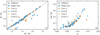 |
Fig. A.1. Comparison of Mi and ΔM of the parametric SN model used in this work (Müller et al. 2016) with the structural parameters M4 and μ4 of the pre-SN models (cf. Ertl et al. 2016). See text for details. |
Appendix B: Fitting formulae
Here we summarise fitting formulae to the compact-object masses of our single and stripped binary star models (Eqs. (B.1)–(B.5) below). Some of these fits are used in the toy population models described in Sect. 5. Below, we define x = MCO/M⊙, i.e. x is the CO core mass at the end of core helium burning. For the fitting functions, we neglect fallback. In order to relate MCO to initial masses, we use spline fits as shown in Fig. 3. The fits to the compact remnant masses are visualised in Fig. B.1 and the fitting functions are as follows.
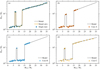 |
Fig. B.1. Piecewise fits to the compact-object masses of single, Case A, Case B, and Case C stripped stars (panels a-d, respectively). For the single stars in panel a, we also show an alternative model fit, “Model (alt.)”. |
Single stars:
 (B.1)
(B.1)
Single stars (alternative):
Employing a parabolic fit function to NS masses beyond the compactness peak instead of the linear fit function used above.
 (B.2)
(B.2)
Case A:
 (B.3)
(B.3)
Case B:
 (B.4)
(B.4)
Case C:
 (B.5)
(B.5)
Appendix C: Schematic mass distribution of compact objects
The NS-mass distribution of single stars in Fig. 9 shows a gap or dearth in the mass range 1.6 − 1.7 M⊙ that is caused by failed SNe from stars in the compactness peak. The existence of such a gap also depends on the exact NS masses of stars just around the compactness peak as we show here. We use two different, piecewise fitting functions to the compact-remnant masses of single stars (Fig. B.1). Model 1 assumes monotonically increasing NS masses with MCO, whereas we fit a parabolic function to the NS masses beyond the compactness peak in Model 2. Assuming a power-law initial mass function with high-mass slope γ = − 2.3 as in Sect. 4.2, we find the NS and BH mass distributions in Fig. C.1.
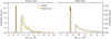 |
Fig. C.1. Mass distribution of NSs and BHs of the two models from Fig. B.1a. Despite the seemingly small difference between the NS masses of the two models, the NS-mass distribution can show distinctly different features around masses that correspond to stars in the compactness peak. A contribution from ECSNe at 1.25 M⊙ has been added, but such SN progenitors are not studied here. |
The NS-mass distributions of Model 1 and 2 show distinctly different features despite the seemingly small changes in the models. A gap is visible in Model 1 at 1.55 M⊙ and is absent in Model 2. Instead of the gap, a bump is observed at 1.50 M⊙, which corresponds to the local minimum in the NS-mass fit of Model 2 at MCO ≈ 10 M⊙. The shift at the lowest NS masses between both models is caused by a slightly different fit to the NS masses before the compactness peak that is hardly visible in Fig. B.1.
All Tables
Initial mass ranges for NS formation in our single and stripped binary star models.
Fractions of NSs to BHs (fNS/BH), single NSs (), single BHs (), single radio pulsars (), single recycled pulsars (), double-neutron-star (DNS) systems with at least one NS formed in an ECSN (), and NSs in binaries after the first SN () in the considered toy population models.
All Figures
|
Fig. 1. Radius evolution of a 13 M⊙ star and definition of Case A, B, and C mass transfer. In this work, we also distinguish between early and late Case B, i.e. mass transfer starting immediately after a star finishes its main-sequence evolution and just before core helium burning, respectively. |
| In the text | |
|
Fig. 2. Core carbon mass fraction XC as a function of (a) initial mass Mini and (b) CO core mass MCO at the end of core helium burning. The initial masses Mini of single stars corresponding to MCO are provided at the top of panel b (cf. Fig. 3). The light-grey shading indicates radiative core carbon burning and the darkish-grey shading indicates radiative core neon burning. The dashed (dotted) lines show the core carbon mass fractions at the end of core helium burning below which our models burn carbon (neon) in their cores radiatively. In panel b, we zoom in on the two branches and the ranges in XC and MCO do not correspond directly to those in panel a. |
| In the text | |
|
Fig. 3. CO core masses MCO at the core-helium exhaustion as a function of initial mass Mini of our single stars and the Case A, B, and C stripped stars. Models leading to BHs and likely experiencing significant fallback are indicated (see Sects. 4.1 and 4.2 for more details). |
| In the text | |
|
Fig. 4. Kippenhahn diagrams of core hydrogen and core helium burning of stars with an initial mass of 17 M⊙. The evolution of a genuine single star (panel a) is contrasted with that of a star that underwent (late) Case B mass transfer (panel b). The blue colour-coding shows energy production by nuclear burning, and the green, yellow, purple, and red hatched regions denote convection, thermohaline mixing, convective overshooting, and semi-convection, respectively. The blue and red dotted lines indicate approximate helium and carbon cores, here defined as the mass coordinate where the helium and carbon mass fractions first exceed 0.5. |
| In the text | |
|
Fig. 5. Compactness ξ2.5 (panel a) and dimensionless central specific entropy sc (panel b) at core collapse as a function of CO core mass MCO. As in Fig. 2, initial masses Mini corresponding to the CO core masses of single stars are shown at the top (cf. Fig. 3), and the light-grey and darker-grey shadings are for radiative core carbon and core neon burning, respectively. |
| In the text | |
|
Fig. 6. Carbon-free (panel a), neon-free (panel b), and iron core mass (panel c) at core collapse as a function of CO core mass MCO. The carbon- and neon-free core masses are defined as those mass coordinates where the carbon and neon mass fraction falls below 10−5, i.e. these core masses (mass coordinates) indicate the bottom of the carbon- and neon-burning layers at core collapse. |
| In the text | |
|
Fig. 7. Gravitational NS mass MNS, grav and BH mass MBH, grav as a function of the initial mass Mini of stars (panel a) and the CO core mass MCO (panel b). The large grey boxes indicate models with potential (here unaccounted for) fallback that may result in weak or failed SNe. The light yellow triangles are for models that have reached their maximum radius before core helium burning and thus cannot undergo Case C mass transfer. They are shown here mainly for completeness. |
| In the text | |
|
Fig. 8. Initial mass cut Mi of SN shock revival (panel a) and mass ΔM = Mf − Mi involved in accretion onto the proto-NS star (see Sect. 2.3) as a function of MCO (panel b), and the resulting SN explosion energy Eexpl as a function of ΔM (panel c). The final NS mass correlates strongly with Mi (cf. Fig. 7b). The vertical dotted line in panel a is the assumed maximum (baryonic) NS mass. |
| In the text | |
|
Fig. 9. Mass functions of NSs and BHs in our default model (top panel) and a model accounting for fallback (bottom panel). The vertical lines show the median masses of the NS and BH mass distributions, and the corresponding values are provided in the figure. Possible LBV phases are only indicated for the single stars. |
| In the text | |
|
Fig. 10. Distribution of (a) explosion energies and (b) nickel masses of single and stripped binary stars. |
| In the text | |
|
Fig. 11. Explosion energy (a), kick velocity (b), and nickel mass (c) as a function of compactness. |
| In the text | |
|
Fig. 12. Supernova-kick distribution of all stars without (panel a) and with (panel b) fallback. Maxwellian distributions are fitted to the data, and their best-fit σ values are provided. |
| In the text | |
|
Fig. 13. Expected changes of intrinsic gravitational-wave merger rates ΔR of our default model with respect to the single, CPS, F12 rapid, and F12 delayed models (panel a), and ratios of detection rates (panel b). The rate differences ΔR are defined such that positive (negative) values imply a higher (lower) rate in our default model compared to the other models. |
| In the text | |
|
Fig. 14. Chirp-mass distributions of NS–NS, BH–NS, and BH–BH mergers for our default, the CPS, and the two F12 models (panel a), and for the default model without fallback (panel b). |
| In the text | |
|
Fig. A.1. Comparison of Mi and ΔM of the parametric SN model used in this work (Müller et al. 2016) with the structural parameters M4 and μ4 of the pre-SN models (cf. Ertl et al. 2016). See text for details. |
| In the text | |
|
Fig. B.1. Piecewise fits to the compact-object masses of single, Case A, Case B, and Case C stripped stars (panels a-d, respectively). For the single stars in panel a, we also show an alternative model fit, “Model (alt.)”. |
| In the text | |
|
Fig. C.1. Mass distribution of NSs and BHs of the two models from Fig. B.1a. Despite the seemingly small difference between the NS masses of the two models, the NS-mass distribution can show distinctly different features around masses that correspond to stars in the compactness peak. A contribution from ECSNe at 1.25 M⊙ has been added, but such SN progenitors are not studied here. |
| In the text | |
Current usage metrics show cumulative count of Article Views (full-text article views including HTML views, PDF and ePub downloads, according to the available data) and Abstracts Views on Vision4Press platform.
Data correspond to usage on the plateform after 2015. The current usage metrics is available 48-96 hours after online publication and is updated daily on week days.
Initial download of the metrics may take a while.