| Issue |
A&A
Volume 682, February 2024
|
|
|---|---|---|
| Article Number | A123 | |
| Number of page(s) | 16 | |
| Section | Stellar structure and evolution | |
| DOI | https://doi.org/10.1051/0004-6361/202347434 | |
| Published online | 12 February 2024 | |
Convective-core overshooting and the final fate of massive stars⋆
1
Heidelberger Institut für Theoretische Studien, Schloss-Wolfsbrunnenweg 35, 69118 Heidelberg, Germany
e-mail: This email address is being protected from spambots. You need JavaScript enabled to view it.
2
Zentrum für Astronomie der Universität Heidelberg, Astronomisches Rechen-Institut, Mönchhofstr. 12-14, 69120 Heidelberg, Germany
3
University of Oxford, St Edmund Hall, Oxford OX1 4AR, UK
Received:
11
July
2023
Accepted:
27
October
2023
Abstract
A massive star can explode in powerful supernova (SN) and form a neutron star, but it may also collapse directly into a black hole. Understanding and predicting the final fate of such stars is increasingly important, for instance, in the context of gravitational-wave astronomy. The interior mixing of stars (in general) and convective boundary mixing (in particular) remain some of the largest uncertainties in their evolution. Here, we investigate the influence of convective boundary mixing on the pre-SN structure and explosion properties of massive stars. Using the 1D stellar evolution code MESA, we modeled single, non-rotating stars of solar metallicity, with initial masses of 5 − 70 M⊙ and convective core step-overshooting of 0.05 − 0.50 pressure scale heights. Stars were evolved until the onset of iron core collapse and the pre-SN models were exploded using a parametric, semi-analytic SN code. We used the compactness parameter to describe the interior structure of stars at core collapse and we found a pronounced peak in compactness at carbon-oxygen core masses of MCO ≈ 7 M⊙, along with generally high compactness at MCO ≳ 14 M⊙. Larger convective core overshooting will shift the location of the compactness peak by 1 − 2 M⊙ to higher MCO. These core masses correspond to initial masses of 24 M⊙ (19 M⊙) and ≳40 M⊙ (≳30 M⊙), respectively, in models with the lowest (highest) convective core overshooting parameter. In both high-compactness regimes, stars are found to collapse into black holes. As the luminosity of the pre-supernova progenitor is determined by MCO, we predict black hole formation for progenitors with luminosities of 5.35 ≤ log(L/L⊙)≤5.50 and log(L/L⊙)≥5.80. The luminosity range of black hole formation from stars in the compactness peak is in good agreement with the observed luminosity of the red supergiant star N6946 BH1, which disappeared without a bright supernova, indicating that it had likely collapsed into a black hole. While some of our models in the luminosity range of log(L/L⊙) = 5.1 − 5.5 do indeed collapse to form black holes, this does not fully explain the lack of observed SN IIP progenitors at these luminosities. This case specifically refers to the “missing red supergiant” problem. The amount of convective boundary mixing also affects the wind mass loss of stars, such that the lowest black hole masses are 15 M⊙ and 10 M⊙ in our models, with the lowest and highest convective core overshooting parameter, respectively. The compactness parameter, central specific entropy, and iron core mass describe a qualitatively similar landscape as a function of MCO, and we find that entropy is a particularly good predictor of the neutron-star masses in our models. We find no correlation between the explosion energy, kick velocity, and nickel mass production with the convective core overshooting value, but we do see a tight relation with the compactness parameter. Furthermore, we show how convective core overshooting affects the pre-supernova locations of stars in the Hertzsprung–Russell diagram (HRD) and the plateau luminosity and duration of SN IIP light curves.
Key words: stars: black holes / stars: general / stars: massive / stars: neutron / supernovae: general
Full Table A.1 is available at the CDS via anonymous ftp to cdsarc.cds.unistra.fr (130.79.128.5) or via https://cdsarc.cds.unistra.fr/viz-bin/cat/J/A+A/682/A123
© The Authors 2024
 Open Access article, published by EDP Sciences, under the terms of the Creative Commons Attribution License (https://creativecommons.org/licenses/by/4.0), which permits unrestricted use, distribution, and reproduction in any medium, provided the original work is properly cited.
This article is published in open access under the Subscribe to Open model. This email address is being protected from spambots. You need JavaScript enabled to view it. to support open access publication.
1. Introduction
The feedback of massive stars via their strong winds, enormous radiation, and powerful supernova (SN) explosions play an important role, for instance, in the evolution of galaxies and the chemical enrichment of the Universe (e.g., Burbidge et al. 1957; Ceverino & Klypin 2009; Langer 2012; Nomoto et al. 2013; Smith 2014). The question of which massive stars explode in SNe and which collapse into black holes (BHs) without bright SNe remains an open question. Many studies have addressed this question by evolving stellar models to their pre-SN stage and exploring their explodability with SN simulations and parameterized SN codes (e.g., Timmes et al. 1996; Woosley et al. 2002, 2020; Heger et al. 2003; Zhang et al. 2008; O’Connor & Ott 2011; Ugliano et al. 2012; Fryer et al. 2012; Pejcha & Thompson 2015; Müller et al. 2016; Ertl et al. 2016; Sukhbold et al. 2016, 2018; Schneider et al. 2021; Laplace et al. 2021; Patton et al. 2022; Aguilera-Dena et al. 2023). However, there are many uncertainties in massive star evolution that could affect the results of such studies (see e.g., Langer 2012; Maeder & Meynet 2012).
One of the most considerable uncertainties in stellar evolution is convective boundary mixing, which is required to explain, for instance, the width of the main sequence in the Hertzsprung–Russell diagram (HRD), as well as eclipsing binary stars and the core masses of stars measured via asteroseismology (e.g., Chiosi et al. 1992; Schroder et al. 1997; Langer 2012; Neiner et al. 2012; Stancliffe et al. 2015; Salaris & Cassisi 2017; Claret & Torres 2019; Pedersen et al. 2021; Jermyn et al. 2022; Burssens et al. 2023). Also, 3D simulations show an additional mixing above the Schwarzschild boundary into the convectively stable layers, which is broadly in agreement with observations (Meakin & Arnett 2007; Horst et al. 2021; Anders et al. 2022; Andrassy et al. 2022).
Convective boundary mixing plays an important role in the evolution of stars (e.g., Schroder et al. 1997; Langer 2012; Salaris & Cassisi 2017; Higgins & Vink 2019). Because of the additional mixing into the convective burning core, there is more fuel to burn and the main sequence lifetime is prolonged. The mixing increases the mean molecular weight in the star resulting in a higher luminosity and cooler effective temperature. More convective boundary mixing causes the core to grow in mass, hence, the star behaves as though it had a higher initial mass. While the effect of convective core overshooting has been extensively studied on the main sequence (e.g., Brott et al. 2011; Schootemeijer et al. 2019), the effects on the later evolutionary stages and, in particular, on the final fates of massive stars and the properties of possible SNe have not been explored in a systematic way.
Convective boundary mixing is essential in linking observations of SN progenitors to theoretical models. To date, tens of SN progenitors have been discovered and there is a tension between the number of observed and expected SN IIP progenitors, known as the “missing red supergiant” (RSG) problem (Smartt 2009). There are no observed SN IIP progenitors with luminosities higher than log(L/L⊙)≈5.1 (Smartt 2009, 2015), whereas RSGs are observed up to luminosities of log(L/L⊙)≈5.5 (Davies et al. 2018). The luminosity threshold of log(L/L⊙)≳5.1 at which no SN IIP progenitors are found is commonly translated to initial masses of ≳18 M⊙ (e.g., Smartt 2009, 2015), but this conversion depends crucially on the applied stellar models and their assumptions, in particular regarding convective boundary mixing (e.g., Farrell et al. 2020). One of the proposed solutions to the missing RSG problem is that RSGs more massive than ≈18 M⊙ collapse into BHs without a bright SN – thus explaining why they are not found in SN searches (Smartt 2009, 2015).
Here, we systematically explore how the extent of convective boundary mixing affects the pre-SN structure, explodability of stars, resulting SN explosion properties, and the masses of the forming neutron stars (NSs) and BHs. We further investigate whether our models may help resolve the missing RSG problem.
This paper is structured as follows. We describe our stellar evolution computations and the applied SN code in Sect. 2. The pre-SN stellar structures of our models with different convective core overshooting values are shown in Sect. 3 and their predicted final fates are described in Sect. 4. We present the compact remnant masses left behind in Sect. 5 and the explosion properties of our models in Sect. 6. In Sect. 7, we show the models at the pre-SN stage in HRD and compare them to observed SN progenitors. We discuss our findings in Sect. 8 and give our conclusions in Sect. 9.
2. Methods
We evolved our set of stellar models using the 1D stellar evolution code MESA (Modules for Experiments in Stellar Astrophysics, Paxton et al. 2011, 2013, 2015). Our grid contains a set of 250 models with initial masses in the range of 5 − 70 M⊙. The evolution is carried out from the zero-age main sequence until the onset of the iron-core collapse (defined as when the infall velocity of the iron core reaches 950 km s−1). Due to the numerical difficulties we encountered, some of the lower mass models (lower than ≈9 M⊙) in our grid could not be evolved this far in MESA. Instead, we used the Tauris et al. (2015) criterion to predict their final fate, namely: models with a final core-mass1 higher than 1.43 M⊙ produce iron core-collapse supernovae (Fe CCSNe), while those with a final core-mass between 1.37 − 1.43 M⊙ give rise to electron capture supernovae (ECSNe) and models with a final core-mass < 1.37 M⊙ form white dwarfs (WD).
Our physics assumptions for MESA models are given in Sect. 2.1 and we introduce our SN code in Sect. 2.2. All MESA details and the data from the analysis with the SN code are given in Appendix A.
2.1. Stellar evolution simulations with MESA
For the evolution of stellar models, we used MESA version 10398. We evolved single, massive, non-rotating stars at solar metallicity (Z = 0.0142, Asplund et al. 2009) with a helium mass fraction of Y = 0.2703. We followed the same setup as in Schneider et al. (2021), but we changed the convective core overshooting parameter αov = dov/HP, with dov being the distance to which the convective boundary mixing extends above the convective core, HP as the pressure-scale height, and αov as the scaling parameter. To simulate convective boundary mixing, we use the step convective core overshooting scheme in MESA with αov values of 0.05, 0.10, 0.15, 0.20, 0.25, 0.30, 0.35, 0.40, 0.45, and 0.50. We assumed convective boundary mixing above convective core-hydrogen and core-helium burning. Convection is treated using the mixing length theory following Henyey et al. (1965), with the mixing length parameter αMLT = 1.8. For stability against convection, we employed the Ledoux criterion. To avoid numerical difficulties for stars approaching the Eddington limit, we enabled MLT++. Semi-convection was applied with an efficiency parameter of αsc = 0.1 and a thermohaline mixing coefficient of 666 was adopted until core-oxygen exhaustion.
For stellar winds, we applied the custom Schneider et al. (2021) wind-mass-loss scheme, which is similar to the “Dutch” wind mass-loss scheme, but with modified metallicity scalings. For cool stars with effective temperatures of log (Teff/K) < 4, we applied the Nieuwenhuijzen & de Jager (1990) wind mass-loss rates. For hot stars with log (Teff/K) > 4, we applied the Vink et al. (2000, 2001) wind mass-loss rates. If the hydrogen mass fraction at the surface drops below 0.4, we applied the Wolf–Rayet (WR) wind mass-loss rates of Nugis & Lamers (2000). We enabled a nuclear burning network of 21 base isotopes, plus 56Co and 60Cr (APPROX21_CR60_PLUS_CO56.NET) in MESA, which covers all main burning stages. The reaction rates of 12C(α, γ)16O are those of Xu et al. (2013). The spatial and temporal evolution of these models is set with the MESA controls varcontrol_target = 10−5 and mesh_delta_coeff = 0.6. We also allowed for the maximum cell size of max_dq = 10−3 .
We computed the gravitational binding energy, Ebind, of the matter above the iron core2 for our models at the onset of iron core collapse. The gravitational binding energy is given as:
 (1)
(1)
the integration is from the iron core mass coordinate, MFe, to the surface of the star, Msurf, m is the mass coordinate and r is the radius at that given mass coordinate.
Models that are left with a hydrogen envelope mass of more than 1 M⊙ at the onset of core-collapse are assumed to produce type IIP SNe, while those with a hydrogen envelope mass of 0.01 − 1 M⊙ are expected to produce SN IIb (Sravan et al. 2019). Progenitor stars with a helium envelope mass of 0.06 − 0.14 M⊙ are assumed to give rise to SN Ib/c (Hachinger et al. 2012).
2.2. Semi-analytic SN code
We analyzed the pre-SN stellar structure of our models that reach iron core collapse (Fe CC) using the semi-analytic parametric supernova code of Müller et al. (2016). The explosion energy Eexpl is a combination of both the nuclear-burning energy and the neutrino-heating energy. We allowed for a maximum NS mass of 2 M⊙, and for models with a remnant mass of more than 2 M⊙, we assumed a direct collapse to a black hole (Müller et al. 2016). All material that is above a mass coordinate where the neutrino heating launches an explosion is then ejected in a supernova explosion (Müller et al. 2016). After the shock revival, if the explosion energy becomes negative at some mass coordinate, fallback material emerges, thereby reducing the ejected mass (Müller et al. 2016). As in Schneider et al. (2021), we assumed a fallback fraction of 50% of the ejected material Mej in such cases. If the accretion of the ejected material onto the proto-neutron star does not stop before it reaches a maximum NS mass of 2 M⊙, a black hole by fallback is formed. For models that launch a successful explosion, a constant asymmetry parameter is assumed and the kick velocity of the NS is calculated as in Schneider et al. (2021).
Following the scalings of Popov (1993), we estimate the plateau luminosity LSN and the duration of the plateau tSN of type IIP SN light curve as:
 (2)
(2)
 (3)
(3)
with R being the radius of the progenitor star at the onset of iron core collapse.
3. Pre-SN stellar structure
3.1. Interplay of convective core overshooting and wind mass loss in the evolution to core collapse
In Fig. 1, we show the HRD of the evolution of a 35 M⊙ star with different convective core overshooting values shown in different colors. The evolution starts at the zero-age main sequence and ends at the onset of iron core collapse (indicated by circles). Black crosses are separated by 105 yr and show that models spend most of their time on the main sequence where the Vink et al. (2000, 2001) mass-loss rates are applied. After the main sequence, the envelope expands, and the star evolves to lower effective temperatures. When the effective temperature of the star reaches log (Teff/K) < 4, we switched to the stronger wind mass-loss rates of Nieuwenhuijzen & de Jager (1990, as also described in Sect. 2). When the surface hydrogen mass fraction drops below Xsurf < 0.4, we applied the WR wind mass-loss rates of Nugis & Lamers (2000), indicated as thick lines.
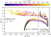 |
Fig. 1. Evolution of initially 35 M⊙ models from the zero-age main sequence until the onset of iron core collapse (filled circles). Colors show models of different convective core overshooting values. Black crosses indicate intervals of 105 yr. The black dotted line marks the transition from the hot to the cool wind mass loss regime at log(Teff/K) = 4. Thick lines show where Wolf-Rayet wind mass-loss rates are applied. |
At the end of the main sequence evolution, the 35 M⊙ model with the highest convective core overshooting value reaches log (L/L⊙)≈5.63 and log (Teff/K)≈4.1. It has a higher luminosity and cooler effective temperature compared to the model with the lowest convective core overshooting value, which at the end of the main sequence reaches values of log (L/L⊙)≈5.53 and log (Teff/K)≈4.5. This is because the model with the highest convective core overshooting has a more extended mixing region and more hydrogen is mixed into the convective burning core, which leads to an increase in the mean molecular weight of the star. Consequently, the star reaches a higher luminosity and builds a more massive He core, leading to a larger radius and lower effective temperature. The 35 M⊙ model with the lowest convective core overshooting value spends its post-main sequence lifetime in the cool wind mass loss regime and ends its life as a red supergiant. The models with a higher convective core overshooting value evolve to higher luminosities because they form more massive cores. The model with the highest convective core overshooting value ends its life with an effective temperature that is 30 times higher than the model with the lowest convective core overshooting. This can be explained by considering the mass loss in stellar winds during their evolution. Models with higher convective core overshooting form more massive cores and are left with a smaller envelope, thus the wind mass loss exposes the hot interiors of the stars and pushes them blueward in the HRD. In the 35 M⊙ model, the Nieuwenhuijzen & de Jager (1990) mass-loss rates are typically ten times stronger than those of Vink et al. (2000, 2001), and three times stronger than the WR rates.
In Fig. 2, we show the total mass lost by stars relative to their initial mass. We find that for initial masses up to 21 M⊙, models with the highest convective core overshooting lose the largest fraction of the mass, while this trend is reversed for initial masses greater than 30 M⊙. For a fixed convective core overshooting value we find a “sweet spot” where the fractional mass loss is the largest. This is found in initial mass models of 21 M⊙ and 35 M⊙ for the highest and lowest convective core overshooting value, respectively. The total mass loss of stars depends on the wind mass-loss rates and for how long stars are subject to which wind mass-loss regime.
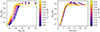 |
Fig. 2. Total mass lost, Mlost, during the evolution relative to the initial mass, Mini, of our entire set of models as a function of the initial mass (left) and CO core mass (right). Colors indicate different convective core overshooting values. |
Because the models with the highest convective core overshooting reach the highest luminosity, their mass-loss rates are the highest throughout all wind mass-loss regimes compared to the models with the lowest convective core overshooting value. During the post-main sequence evolution, models with initial masses ≤21 M⊙ evolve quickly to cool effective temperatures and experience strong wind mass-loss rates until the end of their life. For the 20 M⊙ model with the highest convective core overshooting, the RSG mass-loss rates reach up to 2 × 10⁻⁵ M⊙ yr−1; while for the same initial mass but with the lowest convective core overshooting, RSGs mass loss rates are 6 × 10⁻⁶ M⊙ yr−1. The 20 M⊙ model with the highest convective core overshooting loses up to ≈48% of its initial mass, while this is only 25% for the lowest convective core overshooting model.
Models with initial masses ≥30 M⊙ and the highest convective core overshooting value lose a smaller fraction of their mass compared to those with the lowest convective core overshooting. The 35 M⊙ model with the lowest convective core overshooting spends 0.51 Myr on the cool wind mass-loss regime, being subject to average wind mass-loss rates of ≈3.2 × 10⁻⁵ M⊙ yr−1. In total, it loses 16.1 M⊙ due to RSG winds. For the 35 M⊙ model with the highest convective core overshooting, mass-loss rates in the cool regime on average are ≈2.7 × 10⁻⁵ M⊙ yr−1. Because of its large core, this model has a smaller envelope mass and its hot interiors are exposed after being subject to cool wind mass-loss rates for only 0.32 Myr. The star evolves to higher effective temperatures and becomes a WR star whose wind mass-loss rates are smaller than RSGs winds. The 35 M⊙ model with the highest convective core overshooting is subject to WR winds for 0.1 Myr with average mass-loss rates of ≈2.7 × 10⁻⁶ M⊙ yr−1. Therefore, the total mass lost by the 35 M⊙ model with the highest convective core overshooting is smaller compared to the one with the lowest convective core overshooting.
In the right panel of Fig. 2, we show the total mass lost by stars relative to their initial mass as a function of the CO core mass. We find that up to MCO ≈ 10 M⊙ models with the same MCO lose the same fraction of the initial mass. For models with CO core masses ≥10 M⊙, they reach a plateau-like phase where all models lose ∼50% of their initial mass. Models with MCO > 10 M⊙ and the highest convective core overshooting value lose a smaller fraction of the initial mass because they rapidly evolve through the strongest mass-loss region and become subject to WR winds, as described previously. Based on this relation of the fractional mass loss with the CO core masses for our chosen RSG and WR mass-loss prescription, for a given CO core mass, we can predict rather well how much of the star’s initial mass is going to be lost to stellar winds.
3.2. Core properties
The ultimate fate of stars is determined by the conditions at the end of core helium burning (Chieffi & Limongi 2020; Patton & Sukhbold 2020; Schneider et al. 2021), namely, by the CO core mass and the carbon abundance in the core. During core-helium burning, two different nuclear burning processes take place: the triple-α process in which helium is converted to carbon, and α-captures in which carbon is fused into oxygen via the 12C(α, γ)16O nuclear reaction. Both reaction rates depend on the density, temperature, and amount of helium available in the core. The triple-α reaction rate scales with the third power of the α particle density, while 12C(α, γ)16O scales linearly (Burbidge et al. 1957).
In Fig. 3, we show the core carbon mass fraction of our models at the end of core helium burning as a function of the CO core mass, with colors showing different convective core overshooting values. High-mass models have a lower carbon abundance in the core because they have larger cores of lower (α-particle) density; therefore α-captures onto carbon are favored over triple-α and carbon is converted into oxygen more efficiently (Woosley & Weaver 1995; Brown et al. 1996, 2001).
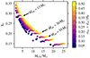 |
Fig. 3. Core carbon mass fraction at the end of core-helium burning as a function of the CO core mass. Colors indicate different convective core overshooting values. We mark the models with initial masses of 13 M⊙, 30 M⊙, and 35 M⊙. |
In models with Mini up to 13 M⊙, the carbon abundance slightly decreases when increasing the convective core overshooting value. That is because with increasing convective core overshooting value, the model behavior resembles that of more massive stars, in the sense that they have more massive CO cores of low density (see Fig. 3).
For models with initial masses 13 − 30 M⊙, wind mass loss becomes more relevant and there is no clear trend with the convective core overshooting value. For the same initial mass model but different convective core overshooting, we find almost the same carbon abundance in the core.
In the most massive stars (Mini > 30 M⊙), models with the highest convective core overshooting tend to have a higher carbon abundance in the CO core. The 35 M⊙ model with the lowest convective core overshooting forms a CO core mass of 11 M⊙ with a carbon abundance of 0.16. The same initial mass model but with the highest convective core overshooting forms a CO core mass of 17 M⊙ with a carbon abundance of 0.18. The high-mass models with the highest convective core overshooting lose most of the hydrogen-rich envelope in stellar winds; consequently, they do not have a hydrogen-burning shell. As a response to the mass loss, the convective core during helium burning decreases in mass, leaving fewer α-particles to be captured onto carbon and produce oxygen. Hence, the carbon abundance in the models with higher convective core overshooting is slightly higher. Similar results are reported by Schneider et al. (2021) and Laplace et al. (2021) for binary-stripped stars.
To describe the core structure and infer the explodability of stars, the compactness parameter is often used. The compactness parameter ξM is defined as:
 (4)
(4)
and is usually evaluated at a mass coordinate of M = 2.5 M⊙ (O’Connor & Ott 2011). Models with a low compactness parameter (ξM ≤ 0.45) tend to produce supernovae and leave behind NSs, while models with a high compactness parameter (ξM ≥ 0.45) are more likely to implode and form BHs (O’Connor & Ott 2011). The compactness parameter follows a pattern as a function of initial mass (Fig. 4) with the first peak at 19 − 24 M⊙, which we refer to as the first compactness peak and a second increase at initial masses of 30 − 40 M⊙, which we refer to as the second compactness peak (O’Connor & Ott 2011; Sukhbold & Woosley 2014; Sukhbold et al. 2018; Patton & Sukhbold 2020; Chieffi & Limongi 2020). For models with the highest convective core overshooting value αov = 0.50, the first increase in compactness is at 19 M⊙ (with a compactness value of 0.65). After the first drop, the second increase in compactness is at the 30 M⊙ model (with a compactness value of 0.59). In the models at the first compactness peak core carbon burning proceeds radiatively, and for the models at the second peak of compactness core neon burning also turns radiative (Schneider et al. 2021).
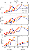 |
Fig. 4. Final compactness parameter, ξ2.5, central specific entropy, sc, iron core mass, MFe and the binding energy above the iron core, Ebind, as a function of initial masses. Colors indicate models for different convective core overshooting parameters. |
In Fig. 4, we show the final compactness parameter, ξ2.5, central specific entropy, sc, the iron core mass, MFe, and the binding energy above the iron core, Ebind, as a function of the initial mass for the models with three different convective core overshooting values (αov = 0.05, 0.30, and 0.50). The central entropy and the iron core masses follow the same trend as the compactness parameter as a function of the initial masses (Schneider et al. 2021; Takahashi et al. 2023). We find that the gravitational binding energy also follows the same non-monotonic trend as compactness as a function of initial mass with a first peak at 19 − 24 M⊙, after the first peak, there is an almost linear increase in the binding energy. By increasing the convective core overshooting parameter, the peaks are shifted to lower initial masses. For models with the lowest convective core overshooting value, the first and second peaks are at Mini ≈ 24 M⊙ and at Mini ≈ 40 M⊙. For the models with the highest convective core overshooting value, the peaks are shifted for 5 M⊙ and 10 M⊙ towards lower initial masses, and are at Mini ≈ 19 M⊙ and Mini ≈ 30 M⊙ for the first and second peak, respectively (see Fig. 4). Lower-mass models with a high convective core overshooting value exhibit a behavior that resembles that of the more massive stars with lower convective core overshooting; thus, they exhibit similar CO core masses.
The final compactness parameter, central specific entropy, the iron core mass, and the binding energy above the iron core are shown in Fig. 5 as a function of their CO core mass. Independently of the convective core overshooting value, we find the first compactness peak at the CO core masses of ∼7 M⊙, and the second peak at ∼14 M⊙; except for the binding energy after MCO ≥ 10 M⊙, there is no second peak but, instead, there is almost a linear increase with MCO (see Fig. 5). However, for the highest convective core overshooting value, there is a slight shift of the peaks toward higher CO core masses, because initially lower mass models with the highest convective core overshooting value form a slightly larger CO core mass than the higher mass models with the lowest convective core overshooting value. We find similar trend and binding energy values when we compute the binding energy of our models above the M4 (the mass coordinate at a specific entropy of s = 4) as our inner mass boundary. Similarly to the initial masses, the central entropy, and the iron core masses follow the same trend as the compactness parameter with the CO core mass (Schneider et al. 2021) as well as the gravitational binding energy. All these quantities hold information about the internal structure of the star and are often used as a proxy to infer the explodability of these stars. Models at MCO ∼ 7 M⊙ have a jump in the binding energy by a factor of three, which shows that these models not only have high compactness, high central specific entropy, and high iron core in addition to a high binding energy that makes it more difficult for these stars to explode. Therefore these models are expected to collapse and form BHs.
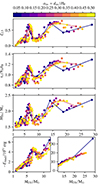 |
Fig. 5. Similar to Fig. 4, but as a function of the CO core mass at the end of core He burning for all models. Colors show models of different convective core overshooting values. The blue, pink, and yellow lines connect models with the same convective core overshooting value for αov = 0.05, 0.30, and 0.50. |
4. Final fates
For the models that do not reach Fe CC, we predicted their final fates based on their CO core mass at the end of core helium burning (see Sect. 2). In Fig. 6, we show the final fates in the MCO − Mini plane. The dark blue region shows models with CO core masses < 1.03 M⊙, which were not able to reach carbon ignition in MESA; therefore, we assume they form CO WD. With the sky-blue region, we show the CO core masses smaller than 1.37 M⊙ where ONeMg WDs are expected to form, the green region is for CO core masses between 1.37 − 1.43 M⊙, where models explode as ECSN, and the pink region for CO core masses > 1.43 M⊙, where models form Fe CCSNe (see Sect. 2 and Tauris et al. 2015).
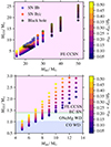 |
Fig. 6. Carbon-oxygen core mass as a function of the initial masses for all our models in initial mass ranges of 5 − 14 M⊙ (bottom), and 14 − 50 M⊙ (top). Colors show the convective core overshooting values. The pink, green, sky-blue, and dark-blue regions show the regions of MCO where iron core-collapse supernovae, electron capture supernovae, and ONeMg white dwarfs are expected, following Tauris et al. (2015). The blue-shaded region shows the CO core masses of models that could not reach carbon ignition thus CO white dwarfs are assumed to form. The blue and red-edged star symbols indicate the models that produce SN IIb and SN Ib/c. Black-edged hexagonal shapes show models that form BHs. |
Models with a high convective core overshooting value form larger CO core masses (see Sect. 3.2). By increasing the convective core overshooting value, models with lower initial mass form Fe CCSNe. The 7 M⊙ model with the lowest convective core overshooting forms a CO core mass of 0.9 M⊙ that becomes a CO WD; while the same initial mass model with the highest convective core overshooting forms a CO core mass of 1.5 M⊙, massive enough to form a Fe CCSN. For the lowest convective core overshooting value, only the models more massive than 10 M⊙ can form a Fe CCSN; while for the highest convective core overshooting value, the 7 M⊙ model produces a Fe CCSN.
Using the parametric supernova code of Müller et al. (2016, as also explained in Sect. 2) we used black-edged hexagons to mark the models that fail to explode and instead collapse into BHs. We find black-hole progenitors at CO core masses of ∼7 M⊙ and > 14 M⊙, which correspond to the first and second compactness peaks. For models with the lowest convective core overshooting value, the 24 M⊙ and the 40 M⊙ models collapse to form BHs. By increasing the convective core overshooting value the models with smaller initial masses form BHs because they have cores of the same compactness as more massive stars with low convective core overshooting. For models with the highest convective core overshooting value, the 19 M⊙ and the 30 M⊙ models collapse into BHs. These models correspond to the models with a high compactness parameter (see Sect. 3.2).
With blue and red star symbols, we show the models that are expected to produce SN IIb and SN Ib/c, respectively. Red supergiant stars by the end of their lives are left with a hydrogen-rich envelope, thus producing SN IIP. We find that by increasing the convective core overshooting value, the type of SN produced changes (Fig. 6). Our high-mass models with the highest convective core overshooting value produce SN IIb and even SN Ib/c. For example, the 27 M⊙ model with the highest convective core overshooting produces SN Ib/c, while the same initial mass model with an intermediate convective core overshooting (αov = 0.30) produce SN IIb and those with αov < 0.30 produce SN IIP. High-mass models with high convective core overshooting lose most of their hydrogen-rich envelope in stellar winds, thereby producing SN IIb or even SN Ib/c, depending on their envelope mass at the onset of Fe CC (Sect. 2).
5. Compact remnant masses
In the left and right panels of Fig. 7, we show the gravitational remnant masses of all models that reach Fe CC as a function of the initial mass and as a function of the CO core masses, respectively. The remnant mass distribution follows a non-monotonic trend as a function of initial masses and CO core masses similar to the compactness parameter, with the first BH formation peak at Mini ≈ 19 − 24 M⊙ and a second BH formation peak at Mini ≈ 30 − 40 M⊙.
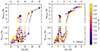 |
Fig. 7. Gravitational neutron-star MNS, grav and black-hole masses MBH, grav as a function of initial mass (left) and CO core mass (right) for our models up to Mini = 50 M⊙. Different convective core overshooting values are indicated by colors and gray boxes indicate models that are expected to experience fallback. |
We see that the 24 M⊙ model with the lowest convective core overshooting value forms a BH of 15 M⊙. With increasing the convective core overshooting value, the 19 M⊙ model forms a BH of 10.2 M⊙. For a higher convective core overshooting value, stars with lower initial masses collapse to form BHs. The same applies to the second peak of BH formation. For models with the lowest convective core overshooting, the 40 M⊙ model forms a BH of 19.2 M⊙, and for the highest convective core overshooting the 30 M⊙ model forms a BH of 15.9 M⊙.
For models that experience a direct collapse into a BH, the mass of the remnant depends on the final mass of the progenitor star. The BH remnant masses have a different order on the first and the second BH formation peaks, which is a consequence of the reversed fractional mass loss (see Fig. 2). For models in the first BH formation peak (Mini < 30 M⊙), the same initial mass model with a higher convective core overshooting value forms a lower mass BH because they have a smaller final mass. For models in the second BH formation peak (Mini > 30 M⊙), the same initial mass model with the highest convective core overshooting forms a more massive BH because they have a higher final mass compared to the same model with a lower convective core overshooting value (see also Fig. 2). The 40 M⊙ model with the lowest convective core overshooting forms a BH of 19.2 M⊙ while the same initial mass model with the highest convective core overshooting forms a BH of 20.9 M⊙ which correspond to the mass of the progenitor star at the onset of Fe CC.
From our models, we predict a minimum BH mass of 10.2 M⊙ if fallback is not taken into account. No LBV mass loss is applied in our models and we overpredict a maximum BH mass of 43.2 M⊙ from the model with Mini = 70 M⊙ model with αov = 0.25.
We find BH formation for the CO core masses ∼7 M⊙ and ≥14 M⊙, as shown on the right panel of Fig. 7, corresponding to the models with a high compactness parameter (see Fig. 5). For models with CO core masses of ∼7 M⊙ and the lowest convective core overshooting value, a BH of 14 M⊙ is formed, while for the same CO core mass but the highest convective core overshooting we form a BH of 10 M⊙. The models with the same CO core mass but higher convective core overshooting value produce BHs of lower masses because the progenitor star had a lower mass initially and has a lower final mass at the end of the evolution (see Fig. 2). For some of the models, the shock cannot propagate throughout the star to launch a successful explosion and hence they experience a partial fallback of the ejected material (see Sect. 2).
In Fig. 8, we show the iron core masses MFe at the end of evolution as a function of the NS masses formed for all the models that successfully explode. In colors, we show the final central entropy of the star. The NS masses scale linearly with the iron core masses. We find that we form NS masses in two distinct branches depending on the central entropy of the star. For the same MFe but lower sc, we will consistently form a NS of lower masses, compared to the same MFe with higher sc. The origin of the two branches remains unclear.
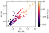 |
Fig. 8. Iron core-mass at the onset of core-collapse as a function of the neutron star mass formed. The colors show the final central specific entropy of the star. |
In Fig. 9, we show the NS masses as a function of their final central specific entropy with colors showing the iron core masses for all our models that launch an explosion. We find a tight relation between the final central specific entropy and the NS mass. Neutron star masses, MNS, follow an exponential function with the central specific entropy of the star sc of the form:
![Mathematical equation: $$ \begin{aligned} M_{\rm NS}=\mathrm{A} \cdot \exp [\mathrm{B}\cdot s_{\rm c}]+\mathrm{C}. \end{aligned} $$](/articles/aa/full_html/2024/02/aa47434-23/aa47434-23-eq5.gif) (5)
(5)
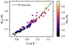 |
Fig. 9. Neutron star mass as a function of the final central specific entropy. The colors indicate the iron-core mass at the onset of Fe CC, and the blue line shows the fit function from Eq. (5). |
Fitting this function to our NS masses we obtain these fitting parameters A = 0.048 ± 0.02, B = 2.76 ± 0.46, and C = 0.88 ± 0.11 (uncertainties are 1σ). Knowing this relation, we can infer the central entropy for a given NS mass.
6. Supernova explosion properties
6.1. Correlation to the compactness parameter
The explosion energy (Eexpl), kick velocity (vkick), and nickel mass production (MNi) are calculated in our models using the parametric SN code of Müller et al. (2016) as described in Sect. 2.2. In Fig. 10, we show these as a function of the compactness parameter of our models. We find that regardless of the convective core overshooting value, these quantities correlate closely with the compactness parameter. These results are in agreement with the models presented by Schneider et al. (2021) for single and binary-stripped stars. These correlations are not surprising as they are built into Müller et al. (2016) formalism and are generally expected for neutrino-driven explosions. The explosion energy is mostly affected by the accreted mass onto the proto-neutron star, therefore we find a tight correlation with the compactness parameter (Schneider et al. 2021). The temperature after the shock explosion directly affects the Ni mass production and the kick velocity is directly computed from the explosion energy hence the correlation (Schneider et al. 2021, 2023). We find that the relation with the explosion energy, kick velocity, and Ni mass production is mainly dependent on the final internal structure of the star (compactness or entropy, see also Schneider et al. 2021, 2023) and Fig. 10. Any supernova will be affected by this internal structure, as it provides the initial condition for the explosion. Different SN models would result in different SN properties, and these correlations are only expected for neutrino-driven SNe. In a magnetically driven engine-like SN model, these correlations would be different.
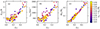 |
Fig. 10. SN explosion properties as a function of the compactness parameter. The explosion energy (a), kick velocity (b), and nickel mass produced (c). The colors indicate the different convective core overshooting values. |
The models with a low compactness value show similar values of explosion energy and for ξ2.5 > 0.2 the explosion energy increases almost linearly (left panel of our Fig. 10 and Fig. 11 in Schneider et al. 2021). Typically, the explosion energy of CCSNe is of the order of ∼1051 erg = 1 B (Kasen & Woosley 2009). Analyzing the explosion properties for a population of stars with a fixed convective core overshooting by applying a Salpeter (1955) IMF we find median values of Eexpl in the range 0.75 − 0.98 B and no trend of Eexpl with convective core overshooting.
After a successful supernova, the neutron star receives a kick due to asymmetries in the explosion. In the middle panel of Fig. 10, we show the kick velocity as a function of the compactness parameter. We find no dependence on the convective core overshooting value, but we see a linear trend with compactness because a higher explosion energy leads to a higher kick velocity (Schneider et al. 2021). By implying a Salpeter (1955) IMF, we find median values of vkick for a population of stars with fixed convective core overshooting in the range 420 − 548 km s−1 (no sigma of a Maxwellian distribution, corresponding approximately to σ = 265 km s−1, Hobbs et al. 2005).
The nickel mass produced in the SN explosion scales linearly with the compactness parameter (see the right panel of our Fig. 10 and Fig. 11 in Schneider et al. 2021). A higher explosion energy leads to a higher post-shock temperature which then directly affects the Ni mass-produced, hence the correlation.
For models producing SN IIP, we find a median value of nickel mass production of MNi ≈ 0.066 M⊙, and for models producing SN IIb, we find a median value of nickel mass production of MNi ≈ 0.101 M⊙. Most of our models explode as SN IIP, and only some of them produce SN IIb and SN Ib/c (see Fig. 6). For a population of stars with fixed convective core overshooting, we find median values of MNi in the range 0.054 − 0.077 M⊙ but no trend of MNi with convective core overshooting. The average inferred observed nickel mass production for SN IIP is ∼0.032 M⊙ and for SN IIb is ∼0.102 M⊙ (Anderson 2019).
6.2. SN ejecta mass and SN IIP light curves
In Fig. 11, we show the SN ejecta mass as a function of the luminosity at the onset of Fe CC for our models that are expected to successfully explode. The SN ejecta mass follows a pattern with initial masses and the luminosity at the onset of Fe CC for different values of convective core overshooting (see Fig. 11). This applies to the initial mass models < 20 M⊙ and log(L/L⊙) < 5.4. Models with the same initial mass but higher convective core overshooting reach a higher luminosity at the onset of Fe CC and have a smaller ejecta mass compared to the same initial mass model with lower convective core overshooting. This is because the low-mass models (Mini < 20 M⊙) with high convective core overshooting lose more mass during the evolution and are left with a smaller envelope that can be ejected during the SN explosion, as compared to the same initial mass models with a smaller convective core overshooting value (Fig. 2). In contrast, for models with higher initial Minit > 20 M⊙ and log(L/L⊙) > 5.4, there is no longer a clear trend seen in the ejecta mass. This is because these models correspond to the ones where the fractional mass loss reaches a turning point (see also Fig. 2). Almost all of these models lose a significant fraction of their initial mass due to winds, affecting the final ejected mass.
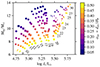 |
Fig. 11. Ejecta mass of our set of models expected to produce a SN explosion as a function of their luminosity at the onset of CC. Markers indicate models with the same initial mass, and numbers are initial masses in solar masses. Different colors show different convective core overshooting values. |
For all the models that are expected to produce SN IIP, we computed the plateau luminosity and the duration of the plateau of the SN light curve, as described in Sect. 2.2. We calibrated the scaling relations to Lp, 0 and tp, 0 for a typically assumed ejecta mass Mej = 10 M⊙, explosion energy Eexpl = 1051 erg, and progenitor radius R = 500 R⊙. The values are expressed in units of plateau luminosity Lp, 0 = 1042 erg s−1 and duration of plateau tp, 0 = 100 days which are typical values for SN IIP (Popov 1993). Models with a higher convective core overshooting value tend to have a shorter duration of the plateau luminosity (Fig. 12). Since the duration of the plateau is proportional to the square root of the ejecta mass (Eq. (3)), the models with high convective core overshooting and small ejecta material have the shortest plateau duration. The plateau luminosity is given by a combination of the explosion energy, the ejected mass, and the radius of the progenitor star (see Eq. (2)). For increasing convective core overshooting values, the ejecta mass generally decreases and the radius of the progenitor star is smaller, with each having the opposite effect on the plateau luminosity. However, the impact of the radius seems to dominate the ejecta mass of our models; thus, we see overall a lower plateau luminosity for models with the highest convective core overshooting (see Fig. 12).
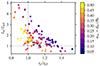 |
Fig. 12. Expected plateau luminosity of SN light-curve as a function of the duration of the plateau for our SN IIP progenitor models. Markers indicate models of the same initial mass, and colors indicate different convective core overshooting values. The black-dotted lines indicate typical values of Lp, 0 = 1042 erg s−1 and tp, 0 = 100 days that are calibrated for RSGs with an Mej = 10 M⊙, Eexpl = 1051 erg, and R = 500 R⊙. |
7. Explosion sites in HRD and missing RSG problem
In Fig. 13, we show the luminosity at the end of core carbon burning as a function of the initial mass (left panel) and as a function of the CO core mass (right panel) for all our models that are expected to produce Fe CCSNe. Models with a higher convective core overshooting value have higher CO core masses and higher luminosities (see Sect. 3). Stars of initial masses between 19 M⊙ to approximately 24 M⊙ and those of Mini ≥ 30 M⊙ collapse to form BHs (see Sect. 5). We find that BH progenitors have similar luminosities at the end of core carbon burning. The low-mass BH progenitor models have luminosities of 5.35 ≤ log(L/L⊙)≤5.47 (see the left panel of Fig. 13). The high-mass BH progenitors have luminosities of log(L/L⊙)≥5.8 corresponding to the second peak of BH formation (left panel of Fig. 13).
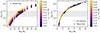 |
Fig. 13. Luminosity of pre-SN models at the end of core-carbon burning, as a function of initial mass (left) and CO core mass (right). The colors represent different values of convective core overshooting and the black circles indicate models that are expected to collapse into BHs. The gray-shaded region is the range of luminosity in which no SN IIP progenitors have been observed so far 5.1 ≤ log(L/L⊙)≤5.5 (Davies & Beasor 2020). The blue line in the right panel shows our fit function to the luminosity and CO core masses of our models (see text). |
As shown in the right panel of Fig. 13, the luminosity at the end of core carbon burning is essentially only a function of the CO core mass. The luminosity of red supergiants can be described by the core mass-luminosity relation. We fit a power law function of the form:
 (6)
(6)
with the fitting parameters A = 4.372 ± 0.005 and B = 1.268 ± 0.006 and 1σ uncertainties.
Using the fit function in Eq. (6), we can infer the CO core mass of the observed pre-SN luminosities of progenitor stars and even predict the final fate. In many studies (Smartt 2009, 2015; Davies & Beasor 2018, 2020) the luminosity of SN progenitors is used to infer their initial mass, but as we show in Fig. 13, there is no clear relation between log(L/L⊙) and Mini. For example, for the luminosity of log(L/L⊙) = 5.1 the progenitor star could be a 13 M⊙ star with the highest convective core overshooting or a 17 M⊙ star with the lowest convective core overshooting. Instead, we can infer their CO core mass more precisely. For example for the SN progenitor with a luminosity of log(L/L⊙) = 5.1 using the fit function we infer a CO core mass of 3.7 M⊙.
The gray-shaded area in Fig. 13 indicates the missing red supergiant region, namely, that there are no observed SN IIP progenitor stars for log(L/L⊙) > 5.1, which may be in tension with the upper luminosity of red supergiants of log(L/L⊙) = 5.5 (Davies et al. 2018). A suggested solution for the missing progenitors of SN IIP is that RSGs more luminous than log(L/L⊙) > 5.1 collapse into BHs (Smartt 2015). However, our simulations predict a successful explosion up to log(L/L⊙) = 5.35 and BH formation in a much narrower range of luminosities of 5.35 ≤ log(L/L⊙)≤5.47.
In Fig. 14, we show an HRD of the entire set of our models at the end of core-carbon burning. The black-edged markers show the models which do not produce a supernova but rather collapse into BHs based on the results from using the parametric SN code of Müller et al. (2016). We compare our models with the observed progenitors of SN IIP from Smartt (2015). The progenitors of SN 2009kr and SN 2009md are removed from the Smartt (2015) sample following Maund et al. (2015). For completeness, we also show the SN 1987A progenitor (Woosley 1988).
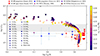 |
Fig. 14. HRD of all our calculated models at the end of core-carbon burning compared to observed supernova progenitors. Symbols show initial masses, and colors indicate different convective core overshooting values. Symbols with black edges are models that are expected to collapse into BHs. As in Fig. 13 the grey shaded region shows the missing RSG region. Red star symbols represent the observed SN IIP progenitor stars, with uncertainties in log(L/L⊙) and log(Teff/K) from Smartt (2015). The red triangles show the upper limits in the luminosity of the observed SN IIP progenitors from Smartt (2015) for which effective temperatures are not known. The red star symbol with blue and black edges shows the SN 2023ixf progenitor from Kilpatrick et al. (2023) and Jencson et al. (2023) respectively. The blue star symbols indicate the observed progenitor stars of type SN IIb as compiled in Yoon et al. (2017). The blue star symbol with red edges indicates the SN 1987A progenitor by Woosley (1988). |
We find a tension between our models and the observed SN IIP progenitors in both luminosity and effective temperature. However, it should be noted that our models are not calibrated to the effective temperatures of RSGs, and the uncertainties in observed SN IIP progenitors are quite large. For example, the uncertainty in the luminosity of the observed SN IIP progenitors extends up to a luminosity of log(L/L⊙)≈5.3. The upper limits in the luminosity of the SN IIP progenitors have values up to log(L/L⊙) = 5.2 which is in the region of the “missing RSG problem”. Our models cannot explain the two least luminous SN IIP progenitors because they are too faint. These are the progenitors of SN2003gd and SN2005cs with luminosities of log(L/L⊙) = 4.3 and log(L/L⊙) = 4.4, respectively. Using the luminosity-CO core mass relation from Eq. (6) we can infer their CO core mass, finding values of ∼0.88 M⊙ and ∼1.04 M⊙ for SN2003gd and SN2005cs, respectively. For such CO core masses, we would predict WD formation. This discrepancy could be resolved if the observed luminosity of SN IIP progenitors were underestimated (see also Sect. 8.4 for a more detailed discussion).
In addition to the already known progenitors of type IIP SNe from Smartt (2015), the progenitor star of SN 2023ixf3 has recently been observed and its progenitor star appears to be a red supergiant that exploded as a type II SN (Kilpatrick et al. 2023; Jencson et al. 2023). Different groups report different progenitor star properties (see Table 1). However, the SN 2023ixf progenitor star may be one of the most luminous progenitors ever detected (Jencson et al. 2023). We show the progenitor star of SN 2023ixf from Kilpatrick et al. (2023) and Jencson et al. (2023) in Fig. 14 by red star markers with blue and black edges respectively. According to Jencson et al. (2023) the progenitor’s luminosity is log(L/L⊙) = 5.1 ± 0.2 which falls in the missing red supergiant regime but it still lies in the region where we predict a successful SNe with luminosity up to log(L/L⊙)≈5.3.
Luminosity and effective temperature of SN 2023ixf progenitor star reported by two different groups.
SN IIb progenitors from Yoon et al. (2017) are indicated with blue star symbols in Fig. 14. Some of our models form SN IIb (see Fig. 6), and comparing them to the observed SN IIb progenitors and the SN 1987A progenitor we find an offset of ≥0.5 dex in luminosity. Our single-star models cannot explain these SN progenitors. This may be expected, given that the progenitor star of SN 1987A is likely a product of binary-star evolution, stellar merger (Podsiadlowski 1992). Similarly, as studied by Yoon et al. (2017), the progenitors of SN IIb most likely are the result of donor stars in binaries that transferred their outer envelope during case B binary mass transfer.
8. Discussion
8.1. Uncertainties in stellar winds
Wind mass-loss rates are not fully understood and it is difficult to model them analytically (Smith 2014). We know that winds influence the evolution of stars, change their internal structure, and affect their final fate (e.g. Chiosi & Maeder 1986; Renzo et al. 2017). For the same initial mass model, but different wind mass loss efficiency or mass loss algorithm, the compactness parameter can change significantly (Renzo et al. 2017). Stronger wind mass loss leads to stars losing more of their envelope and having a higher carbon abundance in the CO core at the end of core helium burning, similar to what we find for our high initial mass models with the highest convective core overshooting. In the most extreme cases, winds remove the entire hydrogen-rich envelope such that stars evolve like binary-stripped stars (cf. Schneider et al. 2021; Laplace et al. 2021). This also affects the compactness and, thus, the explodability of these stars (Patton & Sukhbold 2020; Schneider et al. 2021; Laplace et al. 2021). Enhanced wind mass-loss rates affect the final mass of the progenitor stars, thus affecting the remnant masses left behind. Higher wind mass-loss rates lead to reduced CO-core and thus iron core masses. Hence, the NSs formed will have smaller masses. Depending on how strong the mass-loss rates are, they can change the final outcome, hence changing the number of NSs produced. As shown in Sect. 5, the BH remnant masses are linked to the final mass of the progenitor star. The same initial mass models but with an increased mass-loss rate would form a smaller mass BH. For stronger mass-loss rates, the progenitor models will have a smaller envelope mass and BHs formed by fallback would also have smaller masses.
Models with enhanced wind mass-loss rates would lose more of their envelope mass, thereby producing hydrogen-poor SN explosions (Smith 2014; Renzo et al. 2017) with smaller ejecta masses. A smaller ejected mass for SN IIP shortens the duration of the plateau luminosity, similar to what we found for models with an increased convective core overshooting value in Sect. 6. An enhanced wind mass-loss rate after core-helium burning would not affect the internal structure of the star or the explodability, unless helium or carbon-rich material is lost in stellar winds; in such cases, our models would behave similarly to binary-stripped stars (Schneider et al. 2021; Laplace et al. 2021).
The opposite effect is expected for reduced mass-loss rates, namely: stars would have a larger envelope mass and, consequently, a smaller carbon abundance in the core after core-helium burning. Thus, we would expect them to be on average more difficult to explode. Since their progenitor models would have higher final masses, the BH remnants would be more massive. In the case of a successful SN explosion, for reduced mass-loss rates, models are more likely to produce SN IIP and have a larger ejecta mass.
Some massive stars may experience LBV-like mass loss and eruptions, leading to a sudden increase in luminosity and extended mass loss (Smith 2014). Our models do not take this into account. However, if these instabilities occur before helium depletion, they may change the internal structure of stars by removing the entire hydrogen-rich envelope. The internal structure of these models would be similar to case-B binary-stripped stars (cf. Schneider et al. 2021; Laplace et al. 2021), consistently having a larger carbon abundance in the core and the compactness peak shifted to higher CO core masses. Hence, these models explode more easily and form NSs (Schneider et al. 2021). As reported by Schneider et al. (2021) for the same CO core mass, the remnant masses of BHs are smaller for models that go through case B mass transfer, which also applies to our high mass models if we were to include the eruptive mass loss in our simulations.
8.2. Convective boundary mixing
In our stellar models, we have assumed step convective core overshooting above convective-core hydrogen and helium burning. By introducing the step convective core overshooting in our calculation, we assume an instantaneous mix of chemical elements to a distance, dov, above the convective boundary. The size of the convective core overshooting layer is uncertain and is not well constrained by observations (Schroder et al. 1997; Stancliffe et al. 2015; Salaris & Cassisi 2017). Previous studies have shown that the convective core overshooting parameter is mass-dependent and that higher-mass stars have a larger convective core overshooting parameter (cf. Schroder et al. 1997; Higl et al. 2021; Jermyn et al. 2022; Ahlborn et al. 2022). At present, the exact value of the convective core overshooting for different initial masses has not yet been parametrized. Knowing the mass dependence of the convective core overshooting parameter, we could perform population synthesis simulations to more accurately predict the luminosity of the SN and BH progenitors. Because the luminosity of the BH progenitors is not influenced by the initial mass of the models but only the CO core mass, it would not change the luminosity region where we predict BH formation (cf. Fig. 13).
Because of the steep gradient of the chemical composition above the convective helium-burning core, the convective boundary mixing may be smaller during this phase (Langer 2012; Jermyn et al. 2022). Less convective boundary mixing above the convective-helium burning core would lead to a smaller CO core and also to a higher carbon abundance in the core after helium burning. This would translate to the compactness peak shifting to lower CO core masses, affecting the explodability of stars. For a compactness peak at smaller CO core masses the BH progenitors would have a slightly lower luminosity. The convective-core overshooting on the later burning stages would have the same impact as assuming an increased convective core overshooting value, leading to higher final core masses. However, convective core overshooting on the later burning stages may induce shell mergers (cf. Mocák et al. 2018; Andrassy et al. 2020; Yadav et al. 2020), thereby influencing the explodability (O’Connor & Ott 2011; Sukhbold & Woosley 2014; Schneider et al. 2021), as well as changing the signatures of SN explosions (Andrassy et al. 2020).
8.3. Rotationally induced mixing
Convective core overshooting causes additional mixing of the fresh fuel into the convective burning core, increasing the mass of the core and the luminosity of the star. Similar results are found for rotating stars because of rotationally-induced mixing (cf. Heger et al. 2000; Maeder & Meynet 2000, 2012; Hirschi et al. 2004; Brott et al. 2011; Nguyen et al. 2022). Rotationally-induced mixing has a strong impact on the pre-SN structure and on the type of SN produced (Hirschi et al. 2004). They found that rotation changes the internal structure of stars with initial masses up to 30 M⊙. However, for models more massive than 30 M⊙ the rotation does not play a significant role, since their evolution is mostly dominated by the effects of stellar winds. They show that the rotation influences the carbon abundance in the core, in such a way that highly rotating models have a smaller carbon abundance in the core, but that changes for the most massive stars where the impact of winds dominates that of rotation, similarly to what we found for our models with an increased convective core overshooting value (cf. Fig. 3).
Studies from Fichtner et al. (2022) show that for non-rotating models with initial masses Mini ≤ 25 M⊙, the mass loss is dominated by RSG winds, and stars with Mini ≥ 25 M⊙ experience BSG/LBV and WR winds (see their Fig. A.1). For the non-rotating models, they find a maximum fractional mass loss at the Mini = 25 M⊙. In highly rotating models, this maximum is shifted to lower initial masses, because an increase in rotation makes models stay longer on the RSG branch and lose the highest fraction of their mass. More massive stars become blue supergiants and are subject to the WR winds (Fichtner et al. 2022). Similarly to what we find in our models, with increasing convective core overshooting value, models with the lower initial mass lost the highest fraction of their mass, while the more massive ones evolved to become WR stars where mass-loss rates are weaker.
8.4. Missing RSG problem
We compared observed SN IIP progenitors with our models and found that there is an offset in effective temperature between observations and our models. This is not so surprising given that: (a) the inferred effective temperature from observations of IIP SN progenitors is highly uncertain because of the lack of high-quality data, the effect of interstellar and circumstellar extinction, and the systematic uncertainties in the methods used to derive effective temperatures (e.g., Davies et al. 2013) and (b) our models are not calibrated to reproduce the observed effective temperature of RSGs.
The problem of missing SN IIP progenitors of luminosities of log(L/L⊙) = 5.1 − 5.5 has been investigated extensively. One interpretation is that the red supergiants above log(L/L⊙) = 5.1 collapse to form BHs (Smartt 2015). However, our models predict successful supernovae above this limit and black-hole formation for a much narrower range of luminosities 5.35 ≤ log(L/L⊙)≤5.47 as seen in Fig. 13. Our range of BH formation is in agreement with the one observed disappearing red supergiant star N6946 BH14. Its progenitor star had a luminosity of log(L/L⊙)≈5.3 − 5.5 (Gerke et al. 2015; Kochanek et al. 2008; Adams et al. 2017). This seems to confirm our prediction for the BH formation region. Even after changing one of the most uncertain parameters of stellar evolution, the convective core overshooting parameter, the missing red-supergiant problem remains but in a smaller range of luminosity.
Another possible explanation for the absence of RSGs of log(L/L⊙)≥5.1 could be that these stars lose a large amount of mass during their evolution, and are progenitors of SN IIb. Hydrodynamic instabilities of massive stars during the late burning stages may lead to eruptive mass loss (Yoon & Cantiello 2010; Smith & Arnett 2014). This means that SN progenitor stars may have dust surrounding them, which could make the star appear fainter. For example, the observed luminosities of SN2003gd and SN2005cs are so faint that we infer MCO of 0.88 M⊙ and 1.04 M⊙ from our fit in Eq. (6), respectively. Stars with such low MCO are not expected to lead to SNe but should form WDs instead. There seems to be a need for better constraining the luminosities of the observed SN progenitors (see also Davies & Beasor 2018).
We find that the pre-SN luminosities cannot be directly related to the Mini. For example, for the SN progenitors with a luminosity of log(L/L⊙) = 5.1, its progenitor star could be of the initial mass of range 13 − 17 M⊙ with different convective core overshooting value. Instead, as a function of the CO core mass, they form the same CO core mass ≈3.5 M⊙. Therefore, we urge the community to infer the CO core masses rather than the initial masses from the observed luminosity of SN progenitors.
9. Conclusions
We studied the impact of convective-core overshooting on the evolution and final fate of single massive stars. Using the 1D stellar evolution code MESA, we evolve stars in the mass range of 5 − 70 M⊙ for different step convective core overshooting values of 0.05 − 0.50 HP. The pre-supernova stellar models are analyzed using the parametric supernovae code of Müller et al. (2016).
We find that models with different convective core overshooting values have different evolutionary tracks and the changes persist until the end of their lives. In addition, the explodability, explosion properties, and BH and NS masses are affected by convective core overshooting. We compare our pre-SN models to the observed progenitors of type IIP and IIb SN. Our main findings can be summarized as follows.
-
We find that convective core overshooting affects the final masses of stars differently, depending on their initial masses and mass loss history. Models with initial masses of ≤20 M⊙ and the highest convective core overshooting have a higher fractional mass-loss compared to the same initial mass model with the lowest convective core overshooting. For initial masses of ≥30 M⊙, this trend is reversed and models with the highest convective core overshooting have a smaller fractional mass-loss. Moreover, the factional mass loss reaches a maximum of 50% in stars of initial masses of 20 − 35 M⊙, depending on the convective core overshooting value.
-
The “explodability” and final fates of stars are mostly dominated by the CO core mass, MCO, and the central carbon abundance, XC, at the end of core helium burning. Convective core overshooting mainly affects MCO and less so with respect to XC. Models up to 13 M⊙ with the highest convective core overshooting value have a slightly smaller XC value at the end of core-helium burning, compared to the same model with the lowest convective core overshooting. The most massive star (≥30 M⊙) models with the highest convective core overshooting value tend to have a higher XC in the core. Models with initial masses between 13 − 30 M⊙ show no clear trend of XC with the convective core overshooting parameter.
-
For models with the lowest convective core overshooting, we find a compactness peak at initial masses of ∼24 M⊙ and high compactness for Mini ≥ 40 M⊙. By increasing the convective core overshooting value, the compactness landscape is shifted towards lower initial masses by 5 M⊙ and 10 M⊙ for the first and second peaks, respectively. As a function of the CO core mass, we find the compactness peaks at CO core masses of ≈7 M⊙ and 14 M⊙. Increasing the convective core overshooting value shifts the first compactness peak toward higher CO core masses by 1.3 M⊙, while the second peak of compactness stays constant.
-
The compactness parameter, central specific entropy, iron core mass, and the binding energy above the iron core all follow the same trend with MCO. No matter which criterion for explodability is used, the models at MCO ≈ 7 M⊙ are more difficult to explode and so, they are expected to collapse into BHs.
-
The lowest BH mass is 15 M⊙ for the models with the lowest convective core overshooting value, whereas it is 10.2 M⊙ for models with the highest convective core overshooting value. In the first BH formation peak, models with larger convective core overshooting tend to form lower-mass BHs compared to those with smaller convective core overshooting. In the second BH formation region, this order is reversed and models with the same initial mass but a larger convective core overshooting tend to form higher-mass BHs. This is a direct consequence of the different wind mass loss regimes.
-
We find a close relation of the NS masses with the central specific entropy of the star at the core-collapse.
-
In our models, the explosion energy, Eexpl, kick velocity, vkick, and nickel mass production, MNi, follow almost linear trends with the compactness parameter. In addition, we find no correlation with the convective core overshooting value.
-
The luminosity and the duration of the plateau of SN IIP light curves depend on the radius and ejecta mass of SN progenitors and, thus, on convective core overshooting. Our highest convective core overshooting models tend to have a shorter plateau duration and less luminous light curves.
-
The luminosities log(L/L⊙) of our SN progenitors are solely determined by the CO core mass. We find that BH formation occurs for progenitors with luminosities of 5.35 ≤ log(L/L⊙)≤5.47 from stars with MCO ≈ 7 M⊙ and at log(L/L⊙)≥5.8 from stars with MCO ≥ 14 M⊙ independently of the convective core overshooting value. The former BH formation region is in agreement with the observation of the disappearing star N6946 BH1.
-
Because convective boundary mixing is still very uncertain, we show that relating the log(L/L⊙) of SN IIP progenitors to their initial mass is not straightforward. However, we can infer MCO quite robustly.
We find that convective core overshooting cannot solve the missing red supergiant problem, namely, the lack of detected SN IIP progenitors with log(L/L⊙) = 5.1 − 5.5. However, our models demonstrate that some stars in this luminosity range do indeed collapse into BHs.
Following Tauris et al. (2015), the final core mass is defined as where the helium mass fraction drops below 10%, which corresponds to the CO core mass in our models.
Iron core includes all species with a mass number more than 46. The definition of iron core boundary by MESA is when the 28Si mass-fraction is below 0.01 and the iron mass fraction is more than 0.1.
SN2023ixf occurred during the writing of this paper and the progenitor’s properties are not clear yet with different values on Teff and log(L/L⊙) being reported.
Beasor et al. (2023) claim that the BH candidate shows infrared luminosity, suggesting that the star may not have collapsed, but that it had shed some of its envelope and thus appears dark in bands that were available before JWST. This paper appeared during the refere stage and if the star had indeed not collapsed, this interpretation may need to be revisited.
Acknowledgments
The authors acknowledge support from the Klaus Tschira Foundation. This work has received funding from the European Research Council (ERC) under the European Union’s Horizon 2020 research and innovation program (Grant agreement No. 945806) and is supported by the Deutsche Forschungsgemeinschaft (DFG, German Research Foundation) under Germany’s Excellence Strategy EXC 2181/1-390900948 (the Heidelberg STRUCTURES Excellence Cluster).
References
- Adams, S. M., Kochanek, C. S., Gerke, J. R., Stanek, K. Z., & Dai, X. 2017, MNRAS, 468, 4968 [NASA ADS] [CrossRef] [Google Scholar]
- Aguilera-Dena, D. R., Müller, B., Antoniadis, J., et al. 2023, A&A, 671, A134 [NASA ADS] [CrossRef] [EDP Sciences] [Google Scholar]
- Ahlborn, F., Kupka, F., Weiss, A., & Flaskamp, M. 2022, A&A, 667, A97 [NASA ADS] [CrossRef] [EDP Sciences] [Google Scholar]
- Anders, E. H., Jermyn, A. S., Lecoanet, D., & Brown, B. P. 2022, ApJ, 926, 169 [NASA ADS] [CrossRef] [Google Scholar]
- Anderson, J. P. 2019, A&A, 628, A7 [NASA ADS] [CrossRef] [EDP Sciences] [Google Scholar]
- Andrassy, R., Herwig, F., Woodward, P., & Ritter, C. 2020, MNRAS, 491, 972 [NASA ADS] [CrossRef] [Google Scholar]
- Andrassy, R., Higl, J., Mao, H., et al. 2022, A&A, 659, A193 [NASA ADS] [CrossRef] [EDP Sciences] [Google Scholar]
- Asplund, M., Grevesse, N., Sauval, A. J., & Scott, P. 2009, ARA&A, 47, 481 [NASA ADS] [CrossRef] [Google Scholar]
- Beasor, E. R., Hosseinzadeh, G., Smith, N., et al. 2023, ApJ, submitted [arXiv:2309.16121] [Google Scholar]
- Brott, I., de Mink, S. E., Cantiello, M., et al. 2011, A&A, 530, A115 [NASA ADS] [CrossRef] [EDP Sciences] [Google Scholar]
- Brown, G. E., Weingartner, J. C., & Wijers, R. A. M. J. 1996, ApJ, 463, 297 [NASA ADS] [CrossRef] [Google Scholar]
- Brown, G. E., Heger, A., Langer, N., et al. 2001, New Astron., 6, 457 [NASA ADS] [CrossRef] [Google Scholar]
- Burbidge, E. M., Burbidge, G. R., Fowler, W. A., & Hoyle, F. 1957, Rev. Mod. Phys., 29, 547 [NASA ADS] [CrossRef] [Google Scholar]
- Burssens, S., Bowman, D. M., Michielsen, M., et al. 2023, Nat. Astron., 7, 913 [NASA ADS] [CrossRef] [Google Scholar]
- Ceverino, D., & Klypin, A. 2009, ApJ, 695, 292 [Google Scholar]
- Chieffi, A., & Limongi, M. 2020, ApJ, 890, 43 [NASA ADS] [CrossRef] [Google Scholar]
- Chiosi, C., & Maeder, A. 1986, ARA&A, 24, 329 [NASA ADS] [CrossRef] [Google Scholar]
- Chiosi, C., Bertelli, G., & Bressan, A. 1992, ARA&A, 30, 235 [NASA ADS] [CrossRef] [Google Scholar]
- Claret, A., & Torres, G. 2019, ApJ, 876, 134 [Google Scholar]
- Davies, B., & Beasor, E. R. 2018, MNRAS, 474, 2116 [NASA ADS] [CrossRef] [Google Scholar]
- Davies, B., & Beasor, E. R. 2020, MNRAS, 496, L142 [NASA ADS] [CrossRef] [Google Scholar]
- Davies, B., Kudritzki, R.-P., Plez, B., et al. 2013, ApJ, 767, 3 [Google Scholar]
- Davies, B., Crowther, P. A., & Beasor, E. R. 2018, MNRAS, 478, 3138 [NASA ADS] [CrossRef] [Google Scholar]
- Ertl, T., Janka, H. T., Woosley, S. E., Sukhbold, T., & Ugliano, M. 2016, ApJ, 818, 124 [NASA ADS] [CrossRef] [Google Scholar]
- Farrell, E. J., Groh, J. H., Meynet, G., & Eldridge, J. J. 2020, MNRAS, 494, L53 [NASA ADS] [CrossRef] [Google Scholar]
- Fichtner, Y. A., Grassitelli, L., Romano-Díaz, E., & Porciani, C. 2022, MNRAS, 512, 4573 [NASA ADS] [CrossRef] [Google Scholar]
- Fryer, C. L., Belczynski, K., Wiktorowicz, G., et al. 2012, ApJ, 749, 91 [Google Scholar]
- Gerke, J. R., Kochanek, C. S., & Stanek, K. Z. 2015, MNRAS, 450, 3289 [Google Scholar]
- Hachinger, S., Mazzali, P. A., Taubenberger, S., et al. 2012, MNRAS, 422, 70 [NASA ADS] [CrossRef] [Google Scholar]
- Heger, A., Langer, N., & Woosley, S. E. 2000, ApJ, 528, 368 [NASA ADS] [CrossRef] [Google Scholar]
- Heger, A., Fryer, C. L., Woosley, S. E., Langer, N., & Hartmann, D. H. 2003, ApJ, 591, 288 [CrossRef] [Google Scholar]
- Henyey, L., Vardya, M. S., & Bodenheimer, P. 1965, ApJ, 142, 841 [Google Scholar]
- Higgins, E. R., & Vink, J. S. 2019, A&A, 622, A50 [NASA ADS] [CrossRef] [EDP Sciences] [Google Scholar]
- Higl, J., Müller, E., & Weiss, A. 2021, A&A, 646, A133 [NASA ADS] [CrossRef] [EDP Sciences] [Google Scholar]
- Hirschi, R., Meynet, G., & Maeder, A. 2004, A&A, 425, 649 [NASA ADS] [CrossRef] [EDP Sciences] [Google Scholar]
- Hobbs, G., Lorimer, D. R., Lyne, A. G., & Kramer, M. 2005, MNRAS, 360, 974 [Google Scholar]
- Horst, L., Hirschi, R., Edelmann, P. V. F., Andrássy, R., & Röpke, F. K. 2021, A&A, 653, A55 [NASA ADS] [CrossRef] [EDP Sciences] [Google Scholar]
- Jencson, J. E., Pearson, J., Beasor, E. R., et al. 2023, ApJ, 952, L30 [NASA ADS] [CrossRef] [Google Scholar]
- Jermyn, A. S., Anders, E. H., Lecoanet, D., & Cantiello, M. 2022, ApJ, 929, 182 [NASA ADS] [CrossRef] [Google Scholar]
- Kasen, D., & Woosley, S. E. 2009, ApJ, 703, 2205 [NASA ADS] [CrossRef] [Google Scholar]
- Kilpatrick, C. D., Foley, R. J., Jacobson-Galán, W. V., et al. 2023, ApJ, 952, L23 [NASA ADS] [CrossRef] [Google Scholar]
- Kochanek, C. S., Beacom, J. F., Kistler, M. D., et al. 2008, ApJ, 684, 1336 [NASA ADS] [CrossRef] [Google Scholar]
- Langer, N. 2012, ARA&A, 50, 107 [CrossRef] [Google Scholar]
- Laplace, E., Justham, S., Renzo, M., et al. 2021, A&A, 656, A58 [NASA ADS] [CrossRef] [EDP Sciences] [Google Scholar]
- Maeder, A., & Meynet, G. 2000, ARA&A, 38, 143 [Google Scholar]
- Maeder, A., & Meynet, G. 2012, Rev. Mod. Phys., 84, 25 [Google Scholar]
- Maund, J. R., Fraser, M., Reilly, E., Ergon, M., & Mattila, S. 2015, MNRAS, 447, 3207 [CrossRef] [Google Scholar]
- Meakin, C. A., & Arnett, D. 2007, ApJ, 667, 448 [NASA ADS] [CrossRef] [Google Scholar]
- Müller, B., Heger, A., Liptai, D., & Cameron, J. B. 2016, MNRAS, 460, 742 [Google Scholar]
- Mocák, M., Meakin, C., Campbell, S. W., & Arnett, W. D. 2018, MNRAS, 481, 2918 [CrossRef] [Google Scholar]
- Neiner, C., Mathis, S., Saio, H., et al. 2012, A&A, 539, A90 [NASA ADS] [CrossRef] [EDP Sciences] [Google Scholar]
- Nguyen, C. T., Costa, G., Girardi, L., et al. 2022, A&A, 665, A126 [NASA ADS] [CrossRef] [EDP Sciences] [Google Scholar]
- Nieuwenhuijzen, H., & de Jager, C. 1990, A&A, 231, 134 [NASA ADS] [Google Scholar]
- Nomoto, K., Kobayashi, C., & Tominaga, N. 2013, ARA&A, 51, 457 [CrossRef] [Google Scholar]
- Nugis, T., & Lamers, H. J. G. L. M. 2000, A&A, 360, 227 [NASA ADS] [Google Scholar]
- O’Connor, E., & Ott, C. D. 2011, ApJ, 730, 70 [Google Scholar]
- Patton, R. A., & Sukhbold, T. 2020, MNRAS, 499, 2803 [NASA ADS] [CrossRef] [Google Scholar]
- Patton, R. A., Sukhbold, T., & Eldridge, J. J. 2022, MNRAS, 511, 903 [NASA ADS] [CrossRef] [Google Scholar]
- Paxton, B., Bildsten, L., Dotter, A., et al. 2011, ApJS, 192, 3 [Google Scholar]
- Paxton, B., Cantiello, M., Arras, P., et al. 2013, ApJS, 208, 4 [Google Scholar]
- Paxton, B., Marchant, P., Schwab, J., et al. 2015, ApJS, 220, 15 [Google Scholar]
- Pedersen, M. G., Aerts, C., Pápics, P. I., et al. 2021, Nat. Astron., 5, 715 [NASA ADS] [CrossRef] [Google Scholar]
- Pejcha, O., & Thompson, T. A. 2015, ApJ, 801, 90 [NASA ADS] [CrossRef] [Google Scholar]
- Podsiadlowski, P. 1992, PASP, 104, 717 [CrossRef] [Google Scholar]
- Popov, D. V. 1993, ApJ, 414, 712 [NASA ADS] [CrossRef] [Google Scholar]
- Renzo, M., Ott, C. D., Shore, S. N., & De Mink, S. E. 2017, A&A, 603, A118 [NASA ADS] [CrossRef] [EDP Sciences] [Google Scholar]
- Salaris, M., & Cassisi, S. 2017, R. Soc. Open Sci., 4, 170192 [Google Scholar]
- Salpeter, E. E. 1955, ApJ, 121, 161 [Google Scholar]
- Schneider, F. R. N., Podsiadlowski, P., & Müller, B. 2021, A&A, 645, A5 [NASA ADS] [CrossRef] [EDP Sciences] [Google Scholar]
- Schneider, F. R. N., Podsiadlowski, P., & Laplace, E. 2023, ApJ, 950, L9 [NASA ADS] [CrossRef] [Google Scholar]
- Schootemeijer, A., Langer, N., Grin, N. J., & Wang, C. 2019, A&A, 625, A132 [NASA ADS] [CrossRef] [EDP Sciences] [Google Scholar]
- Schroder, K.-P., Pols, O. R., & Eggleton, P. P. 1997, MNRAS, 285, 696 [NASA ADS] [CrossRef] [Google Scholar]
- Smartt, S. J. 2009, ARA&A, 47, 63 [NASA ADS] [CrossRef] [Google Scholar]
- Smartt, S. J. 2015, PASA, 32, e016 [NASA ADS] [CrossRef] [Google Scholar]
- Smith, N. 2014, ARA&A, 52, 487 [NASA ADS] [CrossRef] [Google Scholar]
- Smith, N., & Arnett, W. D. 2014, ApJ, 785, 82 [NASA ADS] [CrossRef] [Google Scholar]
- Sravan, N., Marchant, P., & Kalogera, V. 2019, ApJ, 885, 130 [NASA ADS] [CrossRef] [Google Scholar]
- Stancliffe, R. J., Fossati, L., Passy, J.-C., & Schneider, F. R. N. 2015, A&A, 575, A117 [NASA ADS] [CrossRef] [EDP Sciences] [Google Scholar]
- Sukhbold, T., & Woosley, S. E. 2014, ApJ, 783, 10 [NASA ADS] [CrossRef] [Google Scholar]
- Sukhbold, T., Ertl, T., Woosley, S. E., Brown, J. M., & Janka, H.-T. 2016, ApJ, 821, 38 [Google Scholar]
- Sukhbold, T., Woosley, S. E., & Heger, A. 2018, ApJ, 860, 93 [NASA ADS] [CrossRef] [Google Scholar]
- Takahashi, K., Takiwaki, T., & Yoshida, T. 2023, ApJ, 945, 19 [NASA ADS] [CrossRef] [Google Scholar]
- Tauris, T. M., Langer, N., & Podsiadlowski, P. 2015, MNRAS, 451, 2123 [NASA ADS] [CrossRef] [Google Scholar]
- Timmes, F. X., Woosley, S. E., & Weaver, T. A. 1996, ApJ, 457, 834 [NASA ADS] [CrossRef] [Google Scholar]
- Ugliano, M., Janka, H.-T., Marek, A., & Arcones, A. 2012, ApJ, 757, 69 [NASA ADS] [CrossRef] [Google Scholar]
- Vink, J. S., de Koter, A., & Lamers, H. J. G. L. M. 2000, A&A, 362, 295 [Google Scholar]
- Vink, J. S., de Koter, A., & Lamers, H. J. G. L. M. 2001, A&A, 369, 574 [NASA ADS] [CrossRef] [EDP Sciences] [Google Scholar]
- Woosley, S. E. 1988, ApJ, 330, 218 [Google Scholar]
- Woosley, S. E., & Weaver, T. A. 1995, ApJS, 101, 181 [Google Scholar]
- Woosley, S. E., Heger, A., & Weaver, T. A. 2002, Rev. Mod. Phys., 74, 1015 [NASA ADS] [CrossRef] [Google Scholar]
- Woosley, S. E., Sukhbold, T., & Janka, H. T. 2020, ApJ, 896, 56 [NASA ADS] [CrossRef] [Google Scholar]
- Xu, Y., Takahashi, K., Goriely, S., et al. 2013, Nucl. Phys. A, 918, 61 [Google Scholar]
- Yadav, N., Müller, B., Janka, H. T., Melson, T., & Heger, A. 2020, ApJ, 890, 94 [NASA ADS] [CrossRef] [Google Scholar]
- Yoon, S.-C., & Cantiello, M. 2010, ApJ, 717, L62 [NASA ADS] [CrossRef] [Google Scholar]
- Yoon, S.-C., Dessart, L., & Clocchiatti, A. 2017, ApJ, 840, 10 [NASA ADS] [CrossRef] [Google Scholar]
- Zhang, W., Woosley, S. E., & Heger, A. 2008, ApJ, 679, 639 [NASA ADS] [CrossRef] [Google Scholar]
Appendix A: Model properties
Properties of all our models used throughout the paper. Explosion properties of models that were not computed to core-collapse are empty.
All Tables
Luminosity and effective temperature of SN 2023ixf progenitor star reported by two different groups.
Properties of all our models used throughout the paper. Explosion properties of models that were not computed to core-collapse are empty.
All Figures
|
Fig. 1. Evolution of initially 35 M⊙ models from the zero-age main sequence until the onset of iron core collapse (filled circles). Colors show models of different convective core overshooting values. Black crosses indicate intervals of 105 yr. The black dotted line marks the transition from the hot to the cool wind mass loss regime at log(Teff/K) = 4. Thick lines show where Wolf-Rayet wind mass-loss rates are applied. |
| In the text | |
|
Fig. 2. Total mass lost, Mlost, during the evolution relative to the initial mass, Mini, of our entire set of models as a function of the initial mass (left) and CO core mass (right). Colors indicate different convective core overshooting values. |
| In the text | |
|
Fig. 3. Core carbon mass fraction at the end of core-helium burning as a function of the CO core mass. Colors indicate different convective core overshooting values. We mark the models with initial masses of 13 M⊙, 30 M⊙, and 35 M⊙. |
| In the text | |
|
Fig. 4. Final compactness parameter, ξ2.5, central specific entropy, sc, iron core mass, MFe and the binding energy above the iron core, Ebind, as a function of initial masses. Colors indicate models for different convective core overshooting parameters. |
| In the text | |
|
Fig. 5. Similar to Fig. 4, but as a function of the CO core mass at the end of core He burning for all models. Colors show models of different convective core overshooting values. The blue, pink, and yellow lines connect models with the same convective core overshooting value for αov = 0.05, 0.30, and 0.50. |
| In the text | |
|
Fig. 6. Carbon-oxygen core mass as a function of the initial masses for all our models in initial mass ranges of 5 − 14 M⊙ (bottom), and 14 − 50 M⊙ (top). Colors show the convective core overshooting values. The pink, green, sky-blue, and dark-blue regions show the regions of MCO where iron core-collapse supernovae, electron capture supernovae, and ONeMg white dwarfs are expected, following Tauris et al. (2015). The blue-shaded region shows the CO core masses of models that could not reach carbon ignition thus CO white dwarfs are assumed to form. The blue and red-edged star symbols indicate the models that produce SN IIb and SN Ib/c. Black-edged hexagonal shapes show models that form BHs. |
| In the text | |
|
Fig. 7. Gravitational neutron-star MNS, grav and black-hole masses MBH, grav as a function of initial mass (left) and CO core mass (right) for our models up to Mini = 50 M⊙. Different convective core overshooting values are indicated by colors and gray boxes indicate models that are expected to experience fallback. |
| In the text | |
|
Fig. 8. Iron core-mass at the onset of core-collapse as a function of the neutron star mass formed. The colors show the final central specific entropy of the star. |
| In the text | |
|
Fig. 9. Neutron star mass as a function of the final central specific entropy. The colors indicate the iron-core mass at the onset of Fe CC, and the blue line shows the fit function from Eq. (5). |
| In the text | |
|
Fig. 10. SN explosion properties as a function of the compactness parameter. The explosion energy (a), kick velocity (b), and nickel mass produced (c). The colors indicate the different convective core overshooting values. |
| In the text | |
|
Fig. 11. Ejecta mass of our set of models expected to produce a SN explosion as a function of their luminosity at the onset of CC. Markers indicate models with the same initial mass, and numbers are initial masses in solar masses. Different colors show different convective core overshooting values. |
| In the text | |
|
Fig. 12. Expected plateau luminosity of SN light-curve as a function of the duration of the plateau for our SN IIP progenitor models. Markers indicate models of the same initial mass, and colors indicate different convective core overshooting values. The black-dotted lines indicate typical values of Lp, 0 = 1042 erg s−1 and tp, 0 = 100 days that are calibrated for RSGs with an Mej = 10 M⊙, Eexpl = 1051 erg, and R = 500 R⊙. |
| In the text | |
|
Fig. 13. Luminosity of pre-SN models at the end of core-carbon burning, as a function of initial mass (left) and CO core mass (right). The colors represent different values of convective core overshooting and the black circles indicate models that are expected to collapse into BHs. The gray-shaded region is the range of luminosity in which no SN IIP progenitors have been observed so far 5.1 ≤ log(L/L⊙)≤5.5 (Davies & Beasor 2020). The blue line in the right panel shows our fit function to the luminosity and CO core masses of our models (see text). |
| In the text | |
|
Fig. 14. HRD of all our calculated models at the end of core-carbon burning compared to observed supernova progenitors. Symbols show initial masses, and colors indicate different convective core overshooting values. Symbols with black edges are models that are expected to collapse into BHs. As in Fig. 13 the grey shaded region shows the missing RSG region. Red star symbols represent the observed SN IIP progenitor stars, with uncertainties in log(L/L⊙) and log(Teff/K) from Smartt (2015). The red triangles show the upper limits in the luminosity of the observed SN IIP progenitors from Smartt (2015) for which effective temperatures are not known. The red star symbol with blue and black edges shows the SN 2023ixf progenitor from Kilpatrick et al. (2023) and Jencson et al. (2023) respectively. The blue star symbols indicate the observed progenitor stars of type SN IIb as compiled in Yoon et al. (2017). The blue star symbol with red edges indicates the SN 1987A progenitor by Woosley (1988). |
| In the text | |
Current usage metrics show cumulative count of Article Views (full-text article views including HTML views, PDF and ePub downloads, according to the available data) and Abstracts Views on Vision4Press platform.
Data correspond to usage on the plateform after 2015. The current usage metrics is available 48-96 hours after online publication and is updated daily on week days.
Initial download of the metrics may take a while.