| Issue |
A&A
Volume 645, January 2021
|
|
|---|---|---|
| Article Number | A90 | |
| Number of page(s) | 16 | |
| Section | Planets and planetary systems | |
| DOI | https://doi.org/10.1051/0004-6361/202039135 | |
| Published online | 19 January 2021 | |
Is TiO emission present in the ultra-hot Jupiter WASP-33b? A reassessment using the improved ExoMol TOTO line list
1
Leiden Observatory, Leiden University,
Postbus 9513,
2300, RA Leiden,
The Netherlands
e-mail: This email address is being protected from spambots. You need JavaScript enabled to view it.
2
Astrophysics Research Centre, School of Mathematics and Physics, Queen’s University Belfast, University Road, Belfast BT7 1NN,
UK
3
Max-Planck-Institut für Astronomie,
Königstuhl 17,
69117 Heidelberg,
Germany
4
School of Physics, Trinity College Dublin, The University of Dublin,
Dublin 2,
Ireland
Received:
10
August
2020
Accepted:
6
November
2020
Abstract
Context. Efficient absorption of stellar ultraviolet and visible radiation by TiO and VO is predicted to drive temperature inversions in the upper atmospheres of hot Jupiters. However, very few inversions or detections of TiO or VO have been reported, and results are often contradictory.
Aims. Using the improved ExoMol TOTO line list, we searched for TiO emission in the dayside spectrum of WASP-33b using the same data in which the molecule was previously detected with an older line list at 4.8σ. We intended to confirm the molecular detection and quantify the signal improvement offered by the ExoMol TOTO line list.
Methods. Data from the High Dispersion Spectrograph on the Subaru Telescope was extracted and reduced in an identical manner to the previous study. Stellar and telluric contamination were then removed. High-resolution TiO emission models of WASP-33b were created that spanned a range of molecular abundances using the radiative transfer code petitRADTRANS, and were subsequently cross-correlated with the data.
Results. We measure a 4.3σ TiO emission signature using the ExoMol TOTO models, corresponding to a WASP-33b orbital velocity semi-amplitude of Kp=252.9−5.3+5.0 km s-1 and a system velocity of vsys=−23.0−4.6+4.7 km s-1. Injection-recovery tests using models based on the new and earlier line lists indicate that if the new models provide a perfect match to the planet spectrum, the significance of the TiO detection should have increased by a factor of ~2.
Conclusions. Although the TiO signal we find is statistically significant, comparison with previous works makes our result too ambiguous to claim a clear-cut detection. Unexpectedly, the new ExoMol TOTO models provide a weaker signal than that found previously, which is offset in Kp-vsys space. This sheds some doubt on both detections, especially in light of a recently published TiO non-detection using a different dataset.
Key words: planets and satellites: atmospheres / planets and satellites: composition / planets and satellites: individual: WASP-33b / techniques: spectroscopic
© ESO 2021
1 Introduction
The first exoplanet discovered orbiting a main-sequence star was not only significant as a milestone in the search for such objects. As a gas-giant planet with a mass comparable to that of Jupiter but an orbital period of less than ten days, 51 Peg b represented a new class of planet with no analog in the Solar System (Mayor & Queloz 1995). The discovery of hundreds of these so-called hot Jupiters with such small orbital separations has naturally raised questions about the effects of intense stellar radiation on planetary atmospheres (Hubeny et al. 2003; Fortney et al. 2008). It is predicted that for sufficiently high levels of stellar irradiation, gaseous TiO and VO can persist in the upper atmospheres of hot Jupiters. Efficient absorption of ultraviolet and visible radiation by these molecules would lead to an inversion in the pressure-temperature profile – that is, an increase in temperature with decreasing pressure. The extent and prevalence of such inversions are important to understanding the various radiative, chemical, and dynamical processes at work in the atmospheres of hot Jupiters.
Evidence for thermal inversions and spectral signatures from TiO and VO are scarce in the literature, and results are often ambiguous and sometimes even contradictory. In particular, the relation between thermal inversions and the presence of TiO and VO is not evident. WASP-121b is an illustrative example. Evans et al. (2017) resolve near-infrared H2O emission in secondary eclipse spectra, resulting in an unambiguous detection of a thermal inversion. While the inversion in WASP-121b is supported by TESS phase curve and eclipse photometry (Daylan et al. 2019; Bourrier et al. 2020), no spectroscopic evidence for TiO has been found (Evans et al. 2018; Merritt et al. 2020). Evidence for VO is present in both eclipse (Evans et al. 2017; Mikal-Evans et al. 2019) and transit (Evans et al. 2018) spectra at low resolution, but not in high-resolution transmission spectra (Merritt et al. 2020). Gibson et al. (2020) detect Fe I in high-resolution transmission spectra and suggest the inversion in WASP-121b may instead be driven by neutral iron.
Similarly, CO emission in low-resolution eclipse observations of WASP-18b indicates the presence of an inversion layer, but no evidence for TiO or VO has been found (Sheppard et al. 2017). Arcangeli et al. (2018) confirm the inversion and suggest that H− opacity mayplay an important role in driving the inversion, instead of TiO or VO. Conversely, WASP-19b has a possible TiO detection but no evidence for a temperature inversion. Sedaghati et al. (2017) report a strong TiO signal in transmission at low resolution, while Espinoza et al. (2019) do not.
Currently, WASP-33b is the only exoplanet with a reported temperature inversion and TiO emission detection based on high-dispersion spectral observations. Orbiting its A5 host star in a 1.2-day period, the ultra-hot Jupiter WASP-33b (Teq ~ 2700 K) is one of the hottest known exoplanets. Haynes et al. (2015) find a temperature inversion necessary to interpret near-infrared Hubble Space Telescope eclipse spectra, attributing excess flux at shorter wavelengths to TiO emission. Using cross-correlation techniques on high-resolution optical spectra taken of the planet’s dayside with the Subaru Telescope, Nugroho et al. (2017) detect TiO in emission at the 4.8σ level, assuming the inverted pressure-temperature profile from Haynes et al. (2015). This is both the first high-resolution TiO or VO detection and the first high-resolution detection of a thermal inversion. However, Herman et al. (2020) analyzed similar quality high-resolution optical transmission and dayside spectra of WASP-33b taken with the Canada–France–Hawaii Telescope (CFHT) and do not detect a TiO signal. More recently, Nugroho et al. (2020) have detected Fe I emission from WASP-33b in the same Subaru data and suggest neutral iron may also contribute to driving the inversion.
In this paper, we used the new and more accurate ExoMol TOTO line list for TiO from McKemmish et al. (2019) to reanalyze the data of WASP-33b from the High Dispersion Spectrograph on Subaru, used by Nugroho et al. (2017) to find TiO emission in its dayside spectrum. We anticipated this improved line list would enable a significantly stronger TiO detection. In Sect. 2 we present this data of WASP-33b and discuss our methodology for detecting TiO in Sect. 3. We present and discuss our tentative detection in Sects. 4 and 5.
2 Subaru data of WASP-33
For our analysis, we used archival spectra1 of WASP-33 taken on 26 October 2015 using the High Dispersion Spectrograph (HDS) on the Subaru Telescope, first presented in Nugroho et al. (2017). A slit width of 0′′.2 provided a resolving power  (Δv = 1.8 km s-1), with a pixel sampling of 0.9 km s-1. Fifty-two observations with integration time 600 s were taken using both the blue and red HDS CCDs covering 6164–7396 and 7685–8810 Å, respectively. The observation midpoints span orbital phases ϕ = 0.207–0.539, with the final 15 exposures taken with the planet in occultation.
The extraction of the one-dimensional HDS spectra is identical to that described in Sects. 2.3 and 2.4 of Nugroho et al. (2017). Bias correction, bad-pixel masking, non-linearity correction, background subtraction, and flat fielding were performed on the blue and red CCD frames using IRAF. Subsequently, 18 blue and 12 red orders were extracted and continuum normalized, and a wavelength solution was determined by comparison with Th-Ar frames. A ~0.1-pixel drift in the wavelength solution was identified by comparing the positions of strong telluric lines over the observing night, and corrected by spline interpolation. A 5σ outlier clipping was then applied to each wavelength bin. A full description of these preliminary reduction steps is given in Nugroho et al. (2017).
While these previous steps are identical to those in the original analysis, Nugroho et al. (2017) performed all further analysis for each order separately. Instead, we combined all blue and red orders into a single spectrum and entirely removed the overlapping wavelength regions, which show poor agreement. These regions amount to 7.5% of the wavelength bins. Although this removes some flexibility in treating particular orders differently, it also simplifies the analysis. In addition to flagging the telluric O2 A and B bands at 7600 and 6900 Å, respectively, we flagged all wavelength bins with a telluric transmission value ≤ 0.98. These two steps result in a further flagging of 7.9 and 4.0% of the wavelength bins, respectively. After dividing each wavelength bin by its median value over all observations, we performed an additional 5σ clipping on each and set all outliers to the bin’s median value.
To further identify and remove tellurics and systematic noise, we performed singular value decomposition (SVD) to deconstruct our data matrix into its constituent components as described in de Kok et al. (2013). We created ten new data matrices in addition to the original, each with a successively weaker SVD component removed. After interpolating each matrix onto a wavelength grid with pixels of width 0.5 km s-1, we performed a single high-pass filter with full width 20.5 km s-1 (41 pixels ) on each observation. We then divided each wavelength bin by its standard deviation over all observations. These last two steps were performed separately on the matrices of each SVD “iteration”.
3 Search for TiO emission
3.1 ExoMol Toto opacities for TiO
Recently, McKemmish et al. (2019) published a new line list for TiO as part of the ExoMol project, which aims to calculate complete, accurate line lists for molecular species of interest to exoplanet spectroscopy (Tennyson & Yurchenko 2012). This ExoMol TOTO line list includes data for all the main TiO isotopologues2, computed using more accurate experimental energy levels. McKemmish et al. (2019) demonstrate the superior quality of their ExoMol TOTO line list for the primary isotopologue 48Ti16O compared tothe Plez (2012) line list (hereafter, Plez12), itself an improvement on the Plez (1998) line list (hereafter, Plez98) used by Nugroho et al. (2017) in their study of WASP-33b. Specifically, they note the improved completeness of the ExoMol TOTO line list, as well as improved positions and strengths of lines when compared to M-dwarf spectra. Pavlenko et al. (2020) show that the ExoMol TOTO line lists for the secondary isotopologues also provide an improvement over the Plez12 line list. We calculated TiO opacities using the ExoMol TOTO line list for each main isotopologue on a high-resolution grid (λ∕Δλ = 106) using the method presented in Appendix A of Mollière et al. (2015), which improves efficiency by computing the contributions of line cores and wing continua on a high- and low-resolution grid, respectively.
3.2 petitRADTRANS TiO emission models
The radiative transfer code petitRADTRANS3 (Mollière et al. 2019) was used to model the TiO emission spectrum of WASP-33b. As input for petitRADTRANS, we adopted the Haynes et al. (2015) pressure-temperature profile with inversion also used by Nugroho et al. (2017), and calculated a corresponding one-dimensional mean molecular weight profile for 46 atmospheric layers from 102 to 10−5 bar using the equilibrium chemistry code described in Appendix A2 of Mollière et al. (2017) assuming a solar metallicity. Both profiles are plotted in the left panel of Fig. 1. We included opacity contributions from all five main TiO isotopologues assuming solar abundances. We created a grid of such models, varying the total TiO volume mixing ratio  from −7.0 to −10.0 in steps of 0.2. The
  emission model, scaled by the stellar continuum, is shown as an example in the right panel of Fig. 1. To maximize any retrieved signal, we broadened these models to the HDS resolving power and performed a high-pass filter to mimic our treatment of the HDS data.
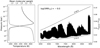 |
Fig. 1 Leftpanel: Haynes et al. (2015) pressure-temperature profile with inversion (solid line) and calculated mean molecular weight profile (dashed line) used to model the TiO emission spectrum of WASP-33b. Right panel: example TiO emission spectrum for WASP-33b assuming a constant
|

3.3 Cross-correlation search for TiO emission
To search for TiO emission in WASP-33b, we cross-correlated each model with the noise residuals of each observation over velocities ±600 km s-1 in steps of 0.5 km s-1 relative to the observatory rest frame. The cross-correlation function (CCF) of each observation was normalized such that values of 0 and 1 correspond to no and full match, respectively, and then median subtracted. This process was performed on the data matrix of each SVD iteration separately, resulting in 11 two-dimensional CCF matrices for each model.
To combine any TiO emission signal over time, we shifted the CCF for each observation to the rest frame of the exoplanet, summed the CCFs for each out-of-occultation observation, and performed another median subtraction. This resulted in a one-dimensional CCF for the entire night of observations. The exoplanet velocity relative to the observatory rest frame at orbital phase ϕ is given by vp (ϕ) = vbary(ϕ) + vsys + Kp sin(2πϕ), where vbary is the velocity of the observatory relative to the Solar System barycenter, vsys is the velocity of the WASP-33 barycenter relative to that of the Solar System, and Kp is the orbital velocity semi-amplitude of WASP-33b. While vbary and the orbital phase for each observation are known, we varied Kp and vsys to allow for deviations from those values reported by Nugroho et al. (2017) and to assess the noise properties of the CCF data. We stacked these one-dimensional CCFs into a Kp -vsys matrix, where each row is the aligned and summed CCF for a given Kp and each column corresponds to a different vsys. We converted the CCF values of each matrix to S∕N values by dividing each row (constant Kp) by its standard deviation. With 11 data matrices (one for each SVD iteration) and 16 model templates, we constructed 176 Kp -vsys matrices.
4 Results
We identified prospective TiO emission by searching for peaks in the Kp -vsys matrices that (1) have velocity values within a 3σ box of the  result from Nugroho et al. (2017), (2) have S∕N ≥ 4σ, and (3) arethe strongest peak on the entire matrix. In the 176 Kp -vsys matrices, we found four peaks that satisfy these criteria, all with
  : peaks with S∕N values of 4.05σ and 4.02σ for the SVD6 and SVD8 data matrices and
  model, and peaks with S∕N values of 4.08σ and 4.03σ for the SVD6 and SVD8 data matrices and
  model.
Although we could not constrain the TiO volume mixing ratio, based on the slightly stronger S∕N values, we adopted the  template as our fiducial model and examined how varying the number of removed SVD components affects theseprospective emission peaks. Figures A.1 and A.2 show the full Kp -vsys matrices for the fiducial model and the data matrix after each successive SVD iteration. The dashed cyan box in each panel denotes the aforementioned 3σ region within which we searched for potential TiO emission, based on the velocities reported by Nugroho et al. (2017). The S∕N and location of the strongest peak on each matrix is noted at the top of each panel and marked by a cyan ring on the matrix. Figures A.3 and A.4 show the same, but with the vsys axis restricted to ±100 km s-1 for clarity. For SVD iterations 6–8 the strongest peak of each matrix falls within the 3σ box around velocities
  . This same emission signal appears present in the Kp -vsys matrices for all SVD iterations and becomes relatively prominent after two iterations of SVD.
To better quantify this, we plotted the S∕N of this emission peak as a function of SVD iteration in Fig. 2. After two SVD iterations the peak exceeds 3σ, which explains its relative prominence in the Kp -vsys matrices for subsequent iterations. The solid markers for SVD iterations 6–8 indicate the peak has the highest S∕N on the Kp -vsys matrix for those iterations. That the strength of the peak falls below 4σ for the SVD7 case explains why it was not initially flagged in our search of all 176 Kp -vsys matrices.
The strongest S∕N value consistent with our search criteria is that at  for the SVD6 data matrix and the
  model. The corresponding Kp -vsys matrix, zoomed to a narrow vsys range for clarity, is shown in Fig. 3. The one-dimensional CCF for Kp = 252.9 km s-1 is shown in the top panel of Fig. 4, recomputed over velocities ±2775 km s-1 from the planet rest frame. We recalculated the noise as the standard deviation of the CCF across this wider velocity range while excluding the central ±25 km s-1 to derive a more robust S∕N = 4.3σ for the peak. The prominence of the central peak is clear over this extensive range of offset velocities.
In the bottom panel of Fig. 4, we sequentially summed the CCFs of all observations in bins, performed a median subtraction, and normalized to S∕N values using the standard deviation outside ±25 km s-1. The first three curves (solid blue, orange, and green) each consist of ten out-of-occultation observations and have peaks with S∕N ~ 2–3σ within 1.0 km s-1 (two pixels) of zero offset velocity. The fourth curve (solid red), consisting of seven out-of-occultation observations, has a S∕N ~ 3σ peak within 1.0 km s-1 of zero offset velocity. The final curve (dashed black) contains only ingress and fully occulted observations, and lacks a similarly distinct, coherent peak close to zero offset velocity. Thus, the presence or absence of the TiO signal seems consistent with the start of occultation.
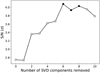 |
Fig. 2 S∕N of the emission peak around |

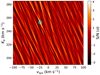 |
Fig. 3 Kp-vsys matrix of S∕N values for the SVD6 data matrix and the |

4.1 Welch’s t-test
To further investigate the significance of this emission signal, we performed a two-sided Welch’s t-test to compare the in- and out-of-trail values of the two-dimensional out-of-occultation CCF matrix for Kp = 252.9 km s-1 (Fig. 5, top panel). Cabot et al. (2019) note that the significance given by the Welch’s t-test is susceptible to overestimation from pixel oversampling. Therefore, we binned the two-dimensional CCF matrix along the velocity axis. Since the resolution element of the HDS data is 1.8 km s-1 and the pixel width is 0.5 km s-1, we averaged the CCF values in three-pixel-wide bins. We adopted in-trail bounds |v| ≤ 1.5 km s-1 and out-of-trail bounds 1.5 km s-1 < |v|≤ 2775 km s-1.
First, we verified that the out-of-trail values are Gaussian using the probability plot shown in the top panel of Fig. 6. Within ±4σ, the out-of-trail CCF values are tightly correlated to a Gaussian normal distribution sampling. The Welch’s t-test gives a two-sided p-value of 1.5 × 10⁻⁵, which corresponds to a 4.3σ rejection of the null hypothesis that the in- and out-of-trail CCF values are drawn from the same distribution. This matches the peak S∕N of the one-dimensional CCF reported in Sect. 4.
The bottom panel of Fig. 6 separately plots the in- and out-of-trail CCF values, clearly showing an overall positive shift of the in-trail values relative to the out-of-trail values. We emphasize that the result of the Welch’s t-test strongly depends on the adopted width of the in-trail region. Our treatment of the data matrices lowers the CCF values immediately surrounding the signal around ± 2–10 km s-1 (Fig. 4, middle panel), lowering the Welch’s t-test significance as more of this region is included.
4.2 Injection-recovery test
We also performed an injection-recovery test to check if we could successfully recover the planet signal. Using the emission peak velocities  determined above, we calculated the relative velocity of WASP-33b at the midpoint of each observation and Doppler shifted the
  model accordingly. We scaled each model emission spectrum to match our data’s normalization, accounting for the planet-to-star full-disk ratio and the mid-observation visible illumination fraction of the planet, which we modeled as a Lambertian sphere. After broadening each model planet spectrum to the resolving power of the data and performing an additional boxcar smoothing to simulate the relatively long 600-s integration time, we added our artificial signal to the pre-flagged HDS data. We thereby injected a TiO emission signal at 1× the expected level for WASP-33b. We subsequently performed the same procedure to reduce stellar, telluric, and systematic noise outlined in Sect. 2, removing six SVD components to mimic the treatment that gave our strongest signal. Using the
  template, broadened and filtered as described in Sect. 3.2, we calculated a Kp -vsys matrix as discussed in Sect. 3.3.
The location of the strongest peak on this matrix is  , matching very closely the injected values. The correspondingly aligned two-dimensional CCF matrix is shown in the bottom panel of Fig. 5, demonstrating how the injected planet signal increases toward occultation as a larger fraction of the dayside becomes visible along our line of sight. The middle panel of Fig. 4 plots the summed one-dimensional CCF on a restricted range for the injected and un-injected cases, which show minimal difference for velocity offsets outside ± 25 km s-1. Within ± 25 km s-1, the shape of thecentral peak and aliasing of the CCF of the injected case matches very closely that of the un-injected case.
As for the un-injected case, we adopted as noise the standard deviation of the one-dimensional CCF over velocities ± 2775 km s-1, excluding the central ± 25 km s-1. We then recover the 1×-injected TiO emission at the 11.2σ level, which is 2.6× as strong as the un-injected case (4.3σ). Assuming our injected model perfectly represents WASP-33b, we would expect a 1× injection at the same location as our tentative detection to result in a doubling of the retrieved S∕N . As our model is not perfect, however, an increase in S∕N of over 100% from a 1× injection-recovery test is to be expected.
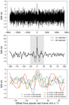 |
Fig. 4 Top panel: one-dimensional out-of-occultation CCF for the |


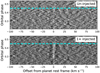 |
Fig. 5 Top panel: two-dimensional CCF matrix for the |


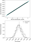 |
Fig. 6 Top panel: probability plot comparing the binned out-of-trail CCF values to a sampling of the normal distribution (black rings). The dashed cyan line is the calculated linear regression. That the correlation so closely follows a linear trend indicates the out-of-trail values are well described by a Gaussian out to ± 4σ . Bottom panel: histogram of the binned in- (dotted line) and out-of-trail (solid line) CCF values. Error bars were calculated as the square root of the individual bin count, normalized by the sample size. A two-sided Welch’s t-test gives a 4.3σ rejection of the null hypothesis that both populations are draw from the same distribution. |
5 Discussion and conclusions
Our detection of a tentative TiO signal in the dayside of WASP-33b is intriguing when compared to similar previous studies. Using the new and more accurate ExoMol TOTO line list for TiO, we find a potential signal at the 4.3σ level in the HDS spectra. Nugroho et al. (2017) used the older Plez98 TiO line list to recover a stronger 4.8σ TiO signal from the same data. Meanwhile, Herman et al. (2020) analyzed CFHT transit and dayside spectra using the Plez12 line list, butdo not detect TiO. There are four possible scenarios: (1) only our TiO detection with the ExoMol TOTO template is valid, (2) only the TiO detection by Nugroho et al. (2017) using the Plez98 line list is valid, (3) both detections are valid, and (4) both detections are false positives. We discuss each below.
5.1 Scenario I: only our detection with ExoMol Toto is valid
Taken in isolation, there are several aspects of our analysis that make our 4.3σ TiO signal compelling. In addition to the statistical significance of the one-dimensional CCF peak (Fig. 4, top panel), the Welch’s t-test presented inSect. 4.1 rejects the hypothesis that the in- and out-of-trail CCF samples are drawn from the same distribution.Furthermore, the injection-recovery test discussed in Sect. 4.2 and shown in the middle panel of Fig. 4 lends confidence to our result, in that the shape of the one-dimensional CCF around the signal peak for the 1×-injected case seems to be a scaled version of that for the un-injected case. Additionally, when the aligned two-dimensional CCF is summed in bins (Fig.4, bottom panel), the presence or absence of the TiO signal seems consistent with the start of occultation.
Nonetheless, we anticipated our analysis of the same HDS data of WASP-33b using the improved ExoMol TOTO line list would yield a stronger TiO detection than the 4.8σ result from Nugroho et al. (2017) using the older Plez98 line list. We initially suspected our weaker detection with a better line list may be partly due to our treatment of the spectral orders. Whereas Nugroho et al. (2017) separately reduced each order and subsequently optimized the number of SYSREM iterations performed on an order-by-order basis using injection-recovery tests, we combined all orders into a single spectrum prior to our comparable step of SVD. As a result, our approach has fewer parameters to optimize and may be inherently unable to maximize the S∕N to a similar degree.
To test whether combining all orders into a single spectrum leads to an inherent decrease in recoverable S∕N , we performed a data reduction similar to that of Nugroho et al. (2017) that treats each spectral order separately. After the extraction, wavelength drift correction, and initial 5σ clipping steps described in Sect. 2, we performed the SYSREM detrending algorithm (Tamuz et al. 2005) independently on each spectral order. After cross-correlation, the CCFs for each order were added with a uniform SYSREM iteration. We chose not to optimize the SYSREM iteration for each order based on injection-recovery tests so as to prevent biasing the signal recovery. However, running SYSREM on each spectral order separately should, in principle, still facilitate a better reduction, assuming the noise varies for different orders. Similarly, the fact that the SYSREM algorithm allows for weighting of individual pixels by their uncertainty during detrending should also enable a more optimized signal recovery. While we readily recover the Nugroho et al. (2017) signal with this methodology when the cross-correlation is performed with their Plez98 models, the results from cross-correlation with the  ExoMol TOTO model are ambiguous and we cannot claim a detection – much less an improvement in signal – using this better-optimized methodology.
Additionally, the Kp and vsys values of our TiO signal are offset compared to previous studies. In Fig. 7, we plot our reported velocity values (circular marker), as well as those from Nugroho et al. (2017) (cross marker), Nugroho et al. (2020) (star marker), and other studies of WASP-33b. In addition to a higher value for Kp , the value our TiO analysis derives for vsys is blue-shifted compared to values presented in previous works. Particularly intriguing is that the error contours indicate a velocity discrepancy between the TiO results of this work and Nugroho et al. (2017), but may indicate agreement between our TiO result and the Fe I detection of Nugroho et al. (2020). We emphasize that all three analyses used the same HDS data of WASP-33b. Also puzzling is the fact that we derive a vsys ~−3 to −5 km s-1 based solely on cross-correlating a rotationally broadened stellar model and the HDS data, which is comparable to previous studies.
5.2 Scenario II: only the Nugroho et al. (2017) detection with Plez98 is valid
In light of these issues, another possible scenario is that the Nugroho et al. (2017) result is valid. While the corresponding values of Kp and vsys that Nugroho et al. (2017) report are indeed in better agreement with previous works (Fig. 7), we were unable to reproduce the same unambiguous detection of TiO emission in WASP-33b using our data treatment with their Plez98 model templates. For reference, we include the corresponding Kp -vsys matrices in Figs. A.5–A.6 and A.7–A.8 for the  cases, whichare the fiducial volume mixing ratios from this work and Nugroho et al. (2017), respectively.
To estimate the recoverability of the TiO signal in WASP-33b with our methodology and the Nugroho et al. (2017) models based on the Plez98 line list, we performed the same ExoMol TOTO injection described in Sect. 4.2 except we cross-correlated with a Plez98 TiO emission template from Nugroho et al. (2017). This way, we could compare the signal lost due to differences in the models. For the recovery, we used the  contrast model presented in Nugroho et al. (2017), broadened and filtered in the same manner as our ExoMol TOTO models to match our treatment of the dataset.
The resulting global peak on the SVD6 Kp -vsys matrix for this Plez98 recovery of injected ExoMol TOTO signal is 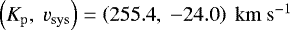 , which is very close to the injected values. This demonstrates that the aforementioned vsys discrepancy between this work and Nugroho et al. (2017) is not caused by differences in the model templates. Indeed, cross-correlating these
  models reveals a relative velocity offset of only 2.0 km s-1, while cross-correlating the
  ExoMol TOTO and
  Plez98 models indicates a relative velocity offset of just 1.5 km s-1. As before, we calculated the noise on the correspondingly aligned one-dimensional CCF between ± 2775 km s-1, excluding the inner ±25 km s-1, to get a 5.1σ detection with the Plez98 model from Nugroho et al. (2017). This represents a 54% loss compared to the 11.2σ signal recovered with our ExoMol TOTO model. Scaling our 4.3σ detection using the ExoMol TOTO models and un-injected data, we estimate the TiO emission present in WASP-33b to be recoverable only at the ≲2σ level using the Plez98 spectral models from Nugroho et al. (2017) with our methodology.
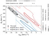 |
Fig. 7 Comparison of various reported values of Kp and vsys for theWASP-33 system. Our result is indicated by the circular marker, along with 1σ and 3σ contoursin black and gray, respectively. The corresponding results from Fig. 14 in Nugroho et al. (2017) for TiO are also plotted, with the location of their S∕N peak denoted by the cross marker and the 1σ and 3σ contours shown in dark and light red. The S∕N peak from the recent Nugroho et al. (2020) Fe I detection is indicated by the star marker, with the 1σ and 3σ contours from the S∕N matrix shown as solid dark blue and solid light blue lines. The vsys = −20 km s-1 lower limit in their analysis caused by stellar pulsations is denoted by the dashed blue line. Previously reported values for vsys (Gontcharov 2006; Collier Cameron et al. 2010) and Kp (Kovács et al. 2013; Smith et al. 2011; Collier Cameron et al. 2010) are shown above and to the right of the plot, with the strokes indicating the reported values, and the extended black and gray bars denoting the 1σ and 3σ errors, respectively. The negative errors for the Kp values are clipped for clarity. |
5.3 Scenario III: both detections are valid
A third possible, but unlikely, scenario is that our TiO emission signal found with the ExoMol TOTO spectral templates and the signature reported by Nugroho et al. (2017) using Plez98 models are both valid. In principle, the comparative completeness of the line lists may influence the retrieved signal. An increased quantity of weak TiO lines in our ExoMol TOTO model template may decrease the effective contrast of the TiO emission, thereby degrading the S∕N . Our fixation of the pressure-temperature profile may also be a contributing factor. Differences in line strengths, line positions, and overall completeness between the ExoMol TOTO and Plez98 line lists may lead to substantially different line profiles even for similar atmospheric models (pressure-temperature profile, mean molecular weight profile, TiO volume mixing ratio, etc.), potentially leading to a weaker detection with the ExoMol TOTO models. Indeed, the normalized cross-correlation of the filtered  Plez98 and ExoMol TOTO models peaks at a value of only 0.28, indicating substantial differences in the spectral models. Similar points are raised by Gandhi et al. (2020) when interpreting a discrepancy in detecting methane using two different line lists.
We attempted to recover our ExoMol TOTO TiO signal using models based on different pressure-temperature profiles to determine whether the signal strength substantially changes for different atmospheric structures. As limiting cases, we adopted fully inverted and non-inverted pressure-temperature profiles that span the same pressure (102 –10−5 bar) and temperature (2700–3700 K) ranges as the Haynes et al. (2015) profile, but vary monotonically with a constant lapse rate. These are the same fully and non-inverted profiles used by Nugroho et al. (2017). We followed the same procedure presented in Sect. 3 to create model spectra with petitRADTRANS for the two alternate atmospheric profiles, and subsequently cross-correlated these models with the processed data. In both the fully and non-inverted cases, varying the total TiO abundance does not lead to significant differences in the final filtered models compared to that for the fiducial abundance of  , so we investigated only with the latter abundance. The fully inverted and non-inverted models recover very similar TiO emission signals, with the former giving a 4.3σ correlation and the latter giving a − 4.4σ anti-correlation at Kp and vsys values consistent with the 4.3σ peak recovered using the Haynes et al. (2015) model. A more exhaustive investigation might determine an optimal inverted pressure-temperature profile that enables the recovery of a stronger TiO emission signal for models based on the ExoMol TOTO line list, butsuch a study is beyond the scope of this work.
Nonetheless, the various points previously raised in this section pose serious challenges to this interpretation that both detections are valid. A degradation in contrast by additional weak lines and our fixation of the pressure-temperature profile would not explain our inability to recover the Nugroho et al. (2017) detection using their Plez98 models. Furthermore, we were unable to find an explanation for the offset in reported vsys .
5.4 Scenario IV: both detections are false positives
The fourth possible scenario is that both TiO emission signals are in fact false positives. Herman et al. (2020) do not find evidence for TiO in either dayside or transmission spectra of WASP-33b. This interpretation has the advantage of explaining the noted discrepancies between this work and Nugroho et al. (2017). Such a scenario would raise questions regarding the current statistical techniques used to evaluate detection significance in high-resolution spectroscopy, as well as highlight the importance of reanalyzing detections using a diverse set of reduction methodologies and spectral models. In the end, further high-resolution spectra may be required to resolve the ambiguity surrounding the presence of TiO in WASP-33b.
Acknowledgements
D.B.S., P.M., and I.A.G.S. acknowledge support from the European Research Council under the European Union’s Horizon 2020 research and innovation program under grant agreement No. 694513. S.K.N. would like to acknowledge support from UK Science Technology and Facility Council grant ST/P000312/1. P.M. acknowledges support from the European Research Council under the European Union’s Horizon 2020 research and innovation program under grant agreement No. 832428. N.P.G. gratefully acknowledges support from Science Foundation Ireland and the Royal Society in the form of a University Research Fellowship.
Appendix A Kp-vsys matrices
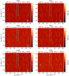 |
Fig. A.1 Kp-vsys matrices of S∕N values for the |

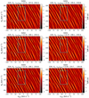 |
Fig. A.3 Same as Fig. A.1, but with the vsys-axis restricted to values within ±100 km s-1 for clarity. While the S∕N peak printedabove each panel refers to that for the full vsys range, the colorbar scaling is based on the S∕N values on this restricted vsys range. |
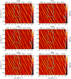 |
Fig. A.5 Kp-vsys matrices of S∕N values for the |

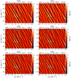 |
Fig. A.7 Kp-vsys matrices of S∕N values for the |

References
- Arcangeli, J., Désert, J.-M., Line, M. R., et al. 2018, ApJ, 855, L30 [NASA ADS] [CrossRef] [Google Scholar]
- Bourrier, V., Kitzmann, D., Kuntzer, T., et al. 2020, A&A, 637, A36 [CrossRef] [EDP Sciences] [Google Scholar]
- Cabot, S. H. C., Madhusudhan, N., Hawker, G. A., & Gandhi, S. 2019, MNRAS, 482, 4422 [NASA ADS] [CrossRef] [Google Scholar]
- Collier Cameron, A., Guenther, E., Smalley, B., et al. 2010, MNRAS, 407, 507 [NASA ADS] [CrossRef] [Google Scholar]
- Daylan, T., Günther, M. N., Mikal-Evans, T., et al. 2019, ArXiv e-prints [arXiv:1909.03000] [Google Scholar]
- de Kok, R. J., Brogi, M., Snellen, I. A. G., et al. 2013, A&A, 554, A82 [NASA ADS] [CrossRef] [EDP Sciences] [Google Scholar]
- Espinoza, N., Rackham, B. V., Jordán, A., et al. 2019, MNRAS, 482, 2065 [Google Scholar]
- Evans, T. M., Sing, D. K., Kataria, T., et al. 2017, Nature, 548, 58 [NASA ADS] [CrossRef] [Google Scholar]
- Evans, T. M., Sing, D. K., Goyal, J. M., et al. 2018, AJ, 156, 283 [NASA ADS] [CrossRef] [Google Scholar]
- Fortney, J. J., Lodders, K., Marley, M. S., & Freedman, R. S. 2008, ApJ, 678, 1419 [NASA ADS] [CrossRef] [Google Scholar]
- Gandhi, S., Brogi, M., Yurchenko, S. N., et al. 2020, MNRAS, 495, 224 [CrossRef] [Google Scholar]
- Gibson, N. P., Merritt, S., Nugroho, S. K., et al. 2020, MNRAS, 493, 2215 [Google Scholar]
- Gontcharov, G. A. 2006, Astron. Astrophys. Trans., 25, 145 [NASA ADS] [CrossRef] [Google Scholar]
- Haynes, K., Mandell, A. M., Madhusudhan, N., Deming, D., & Knutson, H. 2015, ApJ, 806, 146 [NASA ADS] [CrossRef] [Google Scholar]
- Herman, M. K., de Mooij, E. J. W., Jayawardhana, R., & Brogi, M. 2020, AJ, 160, 93 [CrossRef] [Google Scholar]
- Hubeny, I., Burrows, A., & Sudarsky, D. 2003, ApJ, 594, 1011 [NASA ADS] [CrossRef] [Google Scholar]
- Kovács, G., Kovács, T., Hartman, J. D., et al. 2013, A&A, 553, A44 [NASA ADS] [CrossRef] [EDP Sciences] [Google Scholar]
- Mayor, M., & Queloz, D. 1995, Nature, 378, 355 [Google Scholar]
- McKemmish, L. K., Masseron, T., Hoeijmakers, H. J., et al. 2019, MNRAS, 488, 2836 [Google Scholar]
- Merritt, S. R., Gibson, N. P., Nugroho, S. K., et al. 2020, A&A, 636, A117 [CrossRef] [EDP Sciences] [Google Scholar]
- Mikal-Evans, T., Sing, D. K., Goyal, J. M., et al. 2019, MNRAS, 488, 2222 [Google Scholar]
- Mollière, P., van Boekel, R., Dullemond, C., Henning, T., & Mordasini, C. 2015, ApJ, 813, 47 [NASA ADS] [CrossRef] [Google Scholar]
- Mollière, P., van Boekel, R., Bouwman, J., et al. 2017, A&A, 600, A10 [NASA ADS] [CrossRef] [EDP Sciences] [Google Scholar]
- Mollière, P., Wardenier, J. P., van Boekel, R., et al. 2019, A&A, 627, A67 [NASA ADS] [CrossRef] [EDP Sciences] [Google Scholar]
- Nugroho, S. K., Kawahara, H., Masuda, K., et al. 2017, AJ, 154, 221 [NASA ADS] [CrossRef] [Google Scholar]
- Nugroho, S. K., Gibson, N. P., de Mooij, E. J. W., et al. 2020, ApJ, 898, L31 [CrossRef] [Google Scholar]
- Pavlenko, Y. V., Yurchenko, S. N., McKemmish, L. K., & Tennyson, J. 2020, A&A 642, A77 [CrossRef] [EDP Sciences] [Google Scholar]
- Plez, B. 1998, A&A, 337, 495 [NASA ADS] [Google Scholar]
- Plez, B. 2012, Turbospectrum: Code for spectral synthesis [Google Scholar]
- Sedaghati, E., Boffin, H. M. J., MacDonald, R. J., et al. 2017, Nature, 549, 238 [Google Scholar]
- Sheppard, K. B., Mandell, A. M., Tamburo, P., et al. 2017, ApJ, 850, L32 [NASA ADS] [CrossRef] [Google Scholar]
- Smith, A. M. S., Anderson, D. R., Skillen, I., Collier Cameron, A., & Smalley, B. 2011, MNRAS, 416, 2096 [NASA ADS] [CrossRef] [Google Scholar]
- Tamuz, O., Mazeh, T., & Zucker, S. 2005, MNRAS, 356, 1466 [NASA ADS] [CrossRef] [Google Scholar]
- Tennyson, J., & Yurchenko, S. N. 2012, MNRAS, 425, 21 [Google Scholar]
Proposal ID: S15B-090; PI: H. Kawahara.
46Ti16O, 47Ti16O, 48Ti16O, 49Ti16O, 50Ti16O50.
All Figures
|
Fig. 1 Leftpanel: Haynes et al. (2015) pressure-temperature profile with inversion (solid line) and calculated mean molecular weight profile (dashed line) used to model the TiO emission spectrum of WASP-33b. Right panel: example TiO emission spectrum for WASP-33b assuming a constant
|
| In the text | |
|
Fig. 2 S∕N of the emission peak around |
| In the text | |
|
Fig. 3 Kp-vsys matrix of S∕N values for the SVD6 data matrix and the |
| In the text | |
|
Fig. 4 Top panel: one-dimensional out-of-occultation CCF for the |
| In the text | |
|
Fig. 5 Top panel: two-dimensional CCF matrix for the |
| In the text | |
|
Fig. 6 Top panel: probability plot comparing the binned out-of-trail CCF values to a sampling of the normal distribution (black rings). The dashed cyan line is the calculated linear regression. That the correlation so closely follows a linear trend indicates the out-of-trail values are well described by a Gaussian out to ± 4σ . Bottom panel: histogram of the binned in- (dotted line) and out-of-trail (solid line) CCF values. Error bars were calculated as the square root of the individual bin count, normalized by the sample size. A two-sided Welch’s t-test gives a 4.3σ rejection of the null hypothesis that both populations are draw from the same distribution. |
| In the text | |
|
Fig. 7 Comparison of various reported values of Kp and vsys for theWASP-33 system. Our result is indicated by the circular marker, along with 1σ and 3σ contoursin black and gray, respectively. The corresponding results from Fig. 14 in Nugroho et al. (2017) for TiO are also plotted, with the location of their S∕N peak denoted by the cross marker and the 1σ and 3σ contours shown in dark and light red. The S∕N peak from the recent Nugroho et al. (2020) Fe I detection is indicated by the star marker, with the 1σ and 3σ contours from the S∕N matrix shown as solid dark blue and solid light blue lines. The vsys = −20 km s-1 lower limit in their analysis caused by stellar pulsations is denoted by the dashed blue line. Previously reported values for vsys (Gontcharov 2006; Collier Cameron et al. 2010) and Kp (Kovács et al. 2013; Smith et al. 2011; Collier Cameron et al. 2010) are shown above and to the right of the plot, with the strokes indicating the reported values, and the extended black and gray bars denoting the 1σ and 3σ errors, respectively. The negative errors for the Kp values are clipped for clarity. |
| In the text | |
|
Fig. A.1 Kp-vsys matrices of S∕N values for the |
| In the text | |
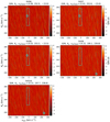 |
Fig. A.2 Same as Fig. A.1, but for SVD iterations 6–10. |
| In the text | |
|
Fig. A.3 Same as Fig. A.1, but with the vsys-axis restricted to values within ±100 km s-1 for clarity. While the S∕N peak printedabove each panel refers to that for the full vsys range, the colorbar scaling is based on the S∕N values on this restricted vsys range. |
| In the text | |
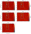 |
Fig. A.4 Same as Fig. A.3, but for SVD iterations 6–10. |
| In the text | |
|
Fig. A.5 Kp-vsys matrices of S∕N values for the |
| In the text | |
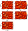 |
Fig. A.6 Same as Fig. A.5, but for SVD iterations 6–10. |
| In the text | |
|
Fig. A.7 Kp-vsys matrices of S∕N values for the |
| In the text | |
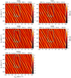 |
Fig. A.8 Same as Fig. A.7, but for SVD iterations 6–10. |
| In the text | |
Current usage metrics show cumulative count of Article Views (full-text article views including HTML views, PDF and ePub downloads, according to the available data) and Abstracts Views on Vision4Press platform.
Data correspond to usage on the plateform after 2015. The current usage metrics is available 48-96 hours after online publication and is updated daily on week days.
Initial download of the metrics may take a while.