| Issue |
A&A
Volume 645, January 2021
|
|
|---|---|---|
| Article Number | A77 | |
| Number of page(s) | 13 | |
| Section | Stellar atmospheres | |
| DOI | https://doi.org/10.1051/0004-6361/202039052 | |
| Published online | 14 January 2021 | |
Monitoring the radio emission of Proxima Centauri
1
CSIC,
Instituto de Astrofísica de Andalucía, Glorieta de la Astronomía S/N,
18008
Granada,
Spain
e-mail: This email address is being protected from spambots. You need JavaScript enabled to view it.
2
INAF, Osservatorio Astrofisico di Catania,
Via S. Sofia 78,
95123 Catania,
Italy
3
School of Physics and Astronomy, Queen Mary University of London,
327 Mile End Road,
London E1 4NS,
UK
4
Departamento de Astronomía, Universidad de Chile, Camino El Observatorio,
1515 Las Condes, Santiago,
Chile
5
Centre for Space Research, Potchefstroom campus, North-West University, Potchefstroom 2531,
South Africa
6
Department of Physics and Astronomy, Faculty of Physical Sciences, University of Nigeria, Carver Building, 1 University Road, Nsukka,
Nigeria
Received:
28
July
2020
Accepted:
2
December
2020
Abstract
We present results from the most comprehensive radio monitoring campaign towards the closest star to our Sun, Proxima Centauri. We report 1.1–3.1 GHz observations with the Australia Telescope Compact Array over 18 consecutive days in April 2017. We detected radio emission from Proxima Centauri for most of the observing sessions, which spanned ~1.6 orbital periods of the planet Proxima b. The radio emission is stronger at the low-frequency band, centered around 1.6 GHz, and is consistent with the expected electron-cyclotron frequency for the known star’s magnetic field intensity of ~600 gauss. The 1.6 GHz light curve shows an emission pattern that is consistent with the orbital period of the planet Proxima b around the star Proxima, with its maxima of emission happening near the quadratures. We also observed two short-duration flares (a few minutes) and a long-duration burst (about three days) whose peaks happened close to the quadratures. We find that the frequency, large degree of circular polarization, change in the sign of circular polarization, and intensity of the observed radio emission are all consistent with expectations from electron cyclotron-maser emission arising from sub-Alfvénic star–planet interaction. We interpret our radio observations as signatures of interaction between the planet Proxima b and its host star Proxima. We advocate for monitoring other dwarf stars with planets to eventually reveal periodic radio emission due to star–planet interaction, thus opening a new avenue for exoplanet hunting and the study of a new field of exoplanet–star plasma interaction.
Key words: instrumentation: interferometers / planet-star interactions / stars: flare / stars: individual: Proxima Centauri / stars: magnetic field
© ESO 2021
1 Introduction
Finding a planet in the habitable zone of the dwarf M star Proxima Centauri (hereafter Proxima) is a major breakthrough in exoplanetary science, especially because the mass and size of the planet are likely similar to those of Earth (Anglada-Escudé et al. 2016). This discovery has triggered a great deal of renewed interest in our close neighbor Proxima, which has been subject to many observational campaigns at different wavelengths of the electromagnetic spectrum, including the detection at millimeter wavelengths of thermal emission from the star itself, and possibly from circumstellar material (Anglada et al. 2017).
Lim et al. (1996) and Slee et al. (2003) reported the detection of radio emission towards Proxima at wavelengths of ~20 cm with the Australian Telescope Compact Array (ATCA). More recently, Bell et al. (2016) reported the non-detection of radio emission from Proxima at 154 MHz, using 12 observations with the Murchison Widefield Array spread between February 10, 2014, and April 30, 2016, placing a 3σ upper limit on the steady-state radio emission from the system in Stokes I of 42.3 mJy beam−1.
The emission detected by Lim et al. (1996) and Slee et al. (2003) presented a degree of circular polarization of nearly 100%, and the authors discussed several possible mechanisms, including the electron cyclotron-maser (ECM) mechanism, but did not provide any details on the origin of the observed emission. The ECM mechanism is also responsible for the highly polarized periodic radio pulses detected in different classes of stars, ranging from hot B-/A-type magnetic stars (Trigilio et al. 2000; Das et al. 2018, 2019a,b; Leto et al. 2019, 2020) to ultra-cool dwarfs and brown dwarfs (Hallinan et al. 2007; Berger et al. 2009; Route & Wolszczan 2012; Kao et al. 2016; Zic et al. 2019).
After the discovery of the exoplanet Proxima Centauri b (hereafter Proxima b) with an orbital period of 11.186 days (Anglada-Escudé et al. 2016), we considered the feasibility of carrying out a monitoring campaign to study Proxima and Proxima b in detail at radio wavelengths. The detection of direct radio emission from the planet Proxima b itself would be very difficult from ground-based radio telescopes because the known emission mechanisms would result in emission that was either with a very low frequency (below the low-frequency end of the radio window set by the Earth’s ionosphere) or very weak (see, e.g., Zarka 2007;Katarzyński et al. 2016). Nevertheless, the interaction of Proxima and its planet Proxima b could produce detectable radio emission at centimeter wavelengths. Zarka (2007) reviewed several possible plasma interactions of exoplanets with their parent stars, and their associated radio emission. In particular, a star–planet interaction can produce ECM emission in a way equivalent to the Jupiter–Io interaction, with the star playing the role of Jupiter and the exoplanet that of Io. The characteristic frequency of the ECM emission is given by the electron gyrofrequency, νg = 2.8 B* MHz, where B* is the stellar surface magnetic field, in gauss. For Jupiter, which has a weak magnetic field (~4.2 G at the equator; Zarka et al. 1996; Connerney et al. 2018), the gyrofrequency falls in the decametric range. In contrast, the magnetic field in the surface of Proxima is B* = 600 ± 150 G (Reiners & Basri 2008), so if the ECM mechanism is at place in the Proxima system as a result of star–planet interaction, emission at a frequency ofνg ≃ 1.7 ± 0.4 GHz should be expected.
2 Observations and data processing
We observedProxima with the Australia Telescope Compact Array (ATCA) in April 12–29, 2017, at a central frequency of 2.1 GHz (corresponding to a wavelength of 14.3 cm). Our observations consisted of 18 observing daily epochs between April 12–29, 2017, encompassing 1.5 orbital cycles (the orbital period of Proxima b is 11.2 days). Each observing session lasted for 3 hours, except on April 24, 2017, that lasted for 12 h, to obtain a full synthesis map of the whole field of view. For all observing sessions, the ATCA was in its 6A configuration, which yields maximum baselines of 5938.8 m. We recorded data using the Compact Array Broadband Backend in CFB_1M mode, which allowed us to observe over a bandwidth of 2 GHz centered at 2.1 GHz, and sampled over 2048 channels of 1 MHz width each; the basic integration time was 10 s. The system yielded auto- and complex cross-correlation products of two perpendicular, linearly polarized signals, from which we obtained full polarization products (all four Stokes parameters). We used the source PKS 1934-638 as bandpass and absolute flux calibrator in all sessions except on April 22, 2017, when it was not visible from ATCA, so we used PKS 0823-500 instead. For complex gain calibration we used the source PKS 1329-665 on April 12, 2017, and PMN J1355-6326 in the rest of sessions. The typical duty cycle for the observations lasted for ≃ 19 min, with 15 min on target (Proxima), 3 min on the complex gain calibrator, and the remaining time spent on antenna slewing. For all observations, we set the phase center at RA = 14h29m33.456s, Dec = −62°40′32.89″ (J2000.0).
We used the Miriad package (Sault et al. 1995) for data editing and calibration. After applying calibration, we exported the visibilities as a measurement set, and performed all imaging steps within the Common Astronomy Software Applications (CASA) package (McMullin et al. 2007). All images presented in this paper were obtained by using multifrequency synthesis and Brigg’s weighting (with robust parameter 0.5, as defined in CASA) on the visibility data, and were deconvolved with the CLEAN algorithm. The resulting synthesized beams of the images covering the whole 2 GHz band were 4.4″ × 3.8″ on April 24, 2017 (when we had a 12-h full observing track on Proxima), and ≃ 20″ × 4″ for the rest of the observing epochs. We obtained maps of total (Stokes I) and circularly polarized flux density (Stokes V = RCP − LCP, where RCP and LCP are right and left circular polarization, respectively) for each day, and in different frequency ranges. We determined the flux densities of Proxima from the peak intensity of each image within one beam of the source position, using the CASA task imfit, and considered the source as detected when that peak was above three times the rms of the map and its location was consistent with the expected position of Proxima. Positional uncertainties are estimated to be ≃ 1″− 4″, considering errors in the absolute astrometry of ATCA at the observed frequency band (Caswell 1998) and in the fit of the peak position (which are on the order of the half-width synthesized beam divided by the signal-to-noise ratio (S/N); Condon et al. 1998). Given the frequency dependence of the emission discussed below, we obtained images at two different frequency ranges: 400 MHz bandwidth, centered at 1.62 GHz (18.5 cm), and 1 GHz bandwidth, centered at 2.52 GHz (11.9 cm).
We searched for variability on short timescales by analyzing the interferometric visibilities, using both the task DFTPL of the AIPS package and the task uvmodelfit of the CASA software package. DFTPL plots the discrete Fourier transform (DFT) of the complex visibilities for any arbitrary point in the sky as a function of time. This task useful for studying the time variability of an unresolved source without the need of making a synthesis map for each time interval. To isolate the emission of Proxima, we made a map of the whole field of view for each observing epoch, and deconvolved it with the CLEAN algorithm, except a tight region around Proxima. Using the resulting CLEAN components as a model of the background sources, we ran the task uvsub of CASA to subtract the model from the visibilities of the corresponding day. Finally, we ran DFTPL on the resulting visibilities using different time intervals. As a trade-off between signal-to-noise ratio and temporal resolution, we examined the data over intervals of a few times 10 sec, which is the duration of a scan. As an independent test, we also ran the task uvmodelfit of CASA on the background-subtracted visibilities for analogous time intervals. This CASA task fits a point source to the visibilities. The results obtained with DFTPL and uvmodelfit are consistent within the uncertainties, and below we discuss only the former.
3 Results
3.1 Long-term radio variability and its correlation with the orbital phase of the planet
Radio emission from the Proxima system is detected in most observing epochs (Table 1). As an illustration, in Fig. 1 we show the maps of the radio continuum emission over the two frequency bands (centered at 1.62 and 2.52 GHz, corresponding to wavelengths of 18.5 and 11.9 cm, respectively) on April 24, 2017. The data taken that day had the best interferometric coverage of all our observational campaigns as this session lasted for 12 h. The location of the emission is consistent, within astrometric uncertainties, with the estimated position of Proxima at the epoch of the observations (Anglada et al. 2017). The total flux density (Stokes I) over the whole 2 GHz bandwidth, was 0.304 ± 0.017 mJy on April 24, which corresponds to a monochromatic radio luminosity of (6.14 ± 0.34) × 1011 erg s−1 Hz−1. Circularly polarized flux density (Stokes V) was also detected on that day, with Proxima being the only source in the field that showed circular polarization above the noise level. The maps in Fig. 1 exclude two short-duration flares, each of ~4 min (Figs. 2f–h), as the variable emission from these flares produces spurious features in the images, when included. The measured flux density, however, was very similar in images with and without the short-duration flares (see Sect. 3.2).
In Figs. 2a–d and Table 1 we show the evolution of the Stokes I and Stokes V data towards the Proxima system, averaged over each observing session and in the two frequency bands. The Stokes I flux density of the low-frequency band, centered at 1.62 GHz (Δν = 400 MHz), has an average value of ≃0.31 mJy over the whole observing period. This value corresponds to an in-band isotropic radio power Pr ≈2.51 × 10²⁰ erg s−1, for an assumed solid angle Ω = 4 π sr. The radio emission of Proxima shows significant variability over the observing campaign, especially at the low-frequency band. The 1.62 GHz Stokes I flux density clearly shows several increases over the quiescent state, each lasting 2–3 days, with an especially long burst during the last 3 days of the observations, which reached ≃5 mJy. This flux density corresponds to a brightness temperature ![Mathematical equation: $T_{\textrm{b}} \gtrsim 3.1\times10^{11}\,[\Delta l/ (0.1 R_{\ast})]^{-2}$](/articles/aa/full_html/2021/01/aa39052-20/aa39052-20-eq1.png) K, where R* = 0.145 R⊙ is the radius of the ProximaCen star, and Δl is the size of the emitting region, which we have normalized to the typical size of a stellar magnetic loop (López Fuentes et al. 2006). In Fig. 3 we show Stokes I images at 1.62 GHz on April 28 (the day with the highest flux density at this frequency), and for the combined data of April 16, 20, 22, 23, and 26. While the source is not detected above the 3σ threshold inany of the individual epochs of the combined image, it clearly shows emission at a level of 0.174 ± 0.038 mJy, indicating the presence of a relatively weak yet quiescent radio emission from Proxima.
K, where R* = 0.145 R⊙ is the radius of the ProximaCen star, and Δl is the size of the emitting region, which we have normalized to the typical size of a stellar magnetic loop (López Fuentes et al. 2006). In Fig. 3 we show Stokes I images at 1.62 GHz on April 28 (the day with the highest flux density at this frequency), and for the combined data of April 16, 20, 22, 23, and 26. While the source is not detected above the 3σ threshold inany of the individual epochs of the combined image, it clearly shows emission at a level of 0.174 ± 0.038 mJy, indicating the presence of a relatively weak yet quiescent radio emission from Proxima.
The low-frequency (1.62 GHz) data is strongly circularly polarized (typically 40–80%), reaching 80–90% during the long burst (Fig. 2 and Table 1). The radio emission also shows a remarkable inversion of its circular polarization, with the Stokes V > 0 for the first half of our observations (until around April 20) and V < 0 from April 24 onwards (panels b and d of Fig. 2). The high degree of circularly polarized emission indicates that the mechanism responsible for the observed emission is coherent.
The variability and degree of circular polarization are significantly lower at the higher frequency band (2.52 GHz; Fig. 2 and Table 1). This is also illustrated in Fig. 4, where we show the ATCA radio spectrum of Proxima over the observing bandwidth (from 1.3 up to 3.1 GHz) for three representative days: April 18, 24, and 28, 2017. We also show the stacked data for the five epochs where no individual detection could be obtained, which indicates the presence of some level of quiescent radio emission. The spectral behavior of the radio emission from Proxima shows evident changes with time. This is particularly conspicuous for the long burst (around April 28, 2017), whose strong total flux density and high fraction of circular polarization (|V |∕I ≳ 80%) are seen only at frequencies ≲2.0 GHz. A fit to a power law with frequency for the data on April 28, 2017, implies a very steep and negative spectral index at frequencies below ≃2.0 GHz (α ≲−7.0;Sν ∝ να). The behavior of this burst appears to be similar in timescale variability, spectral index (very steep, negative), and degree of circular polarization to the emission observed at 1.4 GHz in a previous two-day ATCA campaign (Slee et al. 2003) in May 2000.
We folded our results to the orbital period of Proxima b (Porb = 11.186 days, Anglada-Escudé et al. 2016) to investigate whether the long-term variability of the radio emission could be related to the orbital motion of the planet. We estimated the times that correspond to the conjunctions of the planet (i.e., when the phase is ϕ =0) to obtain the absolute orbital phase of Proxima b. We followed a Monte Carlo approach similar to that applied by Anglada-Escudé et al. (2016), which consists in obtaining a Markov chain of the distribution of orbital parameters derived from the radial velocity solutions, and then propagating the conjunction prediction for each Markov chain Monte Carlo step to a number of integer times the orbital period, Porb. We used all available radial velocities to date (from Anglada-Escudé et al. 2016), as well as 50 new HARPS observations obtained in 2017 within the Red Dots campaign, publicly available at the ESO archive. This procedure generated a distribution for the conjunctions that automatically incorporated the uncertainties on the estimated parameters. During our observing campaign, a conjunction happened on JD 2457864.46 (corresponding to 22:57 UTC on the April 20, 2017), where the uncertainty range of [+21.7, −26.1] h corresponds to the 90% confidence interval.
We show in Fig. 5 the values of Stokes I and V for the low-frequency band (1.62 GHz) data as a function of the orbital phase of Proxima b. The plots show two broad emission peaks in Stokes I and in Stokes V. As a metric for the peak of emission, we used the centroid of each broad emitting region, ϕC = ∑i ϕi Ii∕∑i Ii, where ϕi and Ii correspond to the phase and Stokes I, respectively, of each data point. The resulting centroids correspond to orbital phases ϕC1 = 0.36 ± 0.01 and ϕC2 = 0.81 ± 0.01, separated by about half an orbital period of Proxima b, when the planet was near the positions of the quadratures (i.e., when the planet presents the largest angular separation from the star as seen from Earth). Since we are interested in the analysis of the quiescent emission, we excluded the last three data points of the long-lasting burst in thecalculation of the centroids, which is analyzed separately (see Sect. 4.1.3). If we include the flux density measurements for the long-lasting burst, the second centroid would have a phase of ϕC2 = 0.73. As a metric for the uncertainty on the peak of emission, we used the rms width of each region, w = 2 s, where 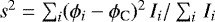 , which yielded values w1 = w2 = 0.18, and are shown as hatched areas in Fig. 5.
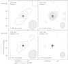 |
Fig. 1 Contour maps of radio continuum emission from the Proxima Centauri system on April 24, 2017. The maps correspond to total (Stokes I) and circularly polarized (Stokes V) flux density, for two bands: 400 MHz centered at 1.62 GHz, and 1 GHz centered at 2.52 GHz. Contour levels are drawn at −2, 2, 4, 6, 8, 10, 12, 14, and 16 times the rms of each map (denoted by σ in each panel). The sign of the Stokes V maps was inverted for better visualization, so solid contours in the two bottom panels actually represent negative values of the circularly polarized flux density. The hatched ellipse in the bottom right corner of each panel represents the half-power contour of the synthesized beams. The cross corresponds to the position of the star Proxima for the observing epoch, obtained from the 1.3 mm ALMA data reported in Anglada et al. (2017), taking into account the proper motion and parallax of the star. |
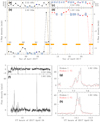 |
Fig. 2 Time evolution of flux density in Proxima. Variation of total (Stokes I; panels a and b) and circularly polarized (Stokes V; panels c and d) flux density as a function of time during our ATCA observing campaign. For each observing session the data is averaged over a bandwidth of 400 MHz and 1 GHz centered at 1.62 GHz [wavelength ≃ 18.5 cm; (b,d)] and 2.52 GHz [≃ 11.9 cm; (a,c)], respectively. Vertical lines indicate 1σ uncertainties for each data point, and blue shaded rectangles are 3σ upper limits for non-detections (in the case of Stokes V, they correspond to upper limits to the absolute value of the flux density). The duration of the observation on April 24, 2017 (12 h), is represented with a horizonal blue bar, while the observing time of the other days (~2 h) is smaller than the symbol size of data points. Dashed orange lines show the quadratures, Q1 and Q2, of Proxima b, with the horizontal orange bars indicating the statistical uncertainty on the determination of the epoch of the quadratures (see text fordetails). The horizontal dashed line in the plot of Stokes I at 1.62 GHz (b) corresponds to a flux density of 0.174 ± 0.038 mJy, obtained by averaging together the data over the five observing sessions where the source was not detected individuallyat that frequency. No map could be obtained at low frequency on April 15, 2017, due to an insufficient number of unflagged visibilities. Panels e and f: variation of Stokes I during April 24, 2017, for data averaged over 20 s intervals. Two short-duration flares are evident at 1.62 GHz (f). Panels g and h: temporal close-up of the two flares. The black and red lines correspond to Stokes I and V, respectively. The sign of Stokes V has been reversed for better visualization. |
Log from our ATCA observations.
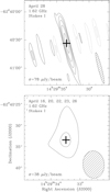 |
Fig. 3 Contour maps of Proxima at 1.62 GHz during maximum and minimum emission. Top panel: emission on April 28, 2017, when the flux density was at its maximum. Contour levels are drawn at −6, −3, 3, 6, 12, 24, and 48 × 78 μJy beam−1, the rms of the map. Bottom panel: map obtained by combining the uv data for the observing epochs when the emission was not detected in each of the individual images (April 16, 20, 22, 23, and 26, 2017). Contour levels are drawn at −2, 2, and 4 × 38 μJy beam−1, the rms of the map. In both maps the solid and dotted contours represent positive and negative levels, respectively. |
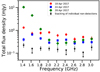 |
Fig. 4 Illustration of the day-to-day radio spectral evolution of Proxima. Data correspond to the total flux density (Stokes I) on April 18 (circles), April 24 (squares), and April 28 (diamonds) over the whole observing bandwidth, averaged every 200 MHz. For comparison, we also show the result of stacking the data corresponding to the five individual observing epochs where there was no detection (data of April 16, 20, 22, 23, and 26), drawn as stars. Arrows indicate 3σ upper limits. |
3.2 Short-term radio variability
The emission from the Proxima system also displayed intra-day variability, as shown in Figs. 2e–h, where we present the observations averaged over 20 s intervals. On April 24, 2017, there are two strong short-duration flares, detected only in the low-frequency band (1.62 GHz), with peaks at 07:45:10 UT (24.323 Apr) and 14:06:30 UT (24.5875 Apr). Their peak flux densities (~25 and ~45 mJy) correspond to about 100 and 200 times the average flux density value in the rest of the observing session. A possibly similar short-duration strongly polarized flare was detected at 1.4 GHz on 1991 August 31, 1991 (Lim et al. 1996), but apparently caught at its peak (~20 mJy) or in its decaying phase.
The duration of these flares (estimated as the time where the flux density exceeds ~2 mJy) is about 4 min in each event, showing a main and a secondary peak separated by about 2 min, and hints of substructure at shorter temporal scales of about 40 s. The two short-duration flares are also evident in the low-frequency V data (Fig. 2), and show a very high degree of circular polarization (|V |∕I = 80–100%). On the contrary, the high-frequency band centered on 2.52 GHz does not show any evidence of those short-duration flares.
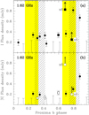 |
Fig. 5 Flux density light curve of Proxima (1.62 GHz) folded to the orbital period of the planet Proxima b, covering ~1.6 orbital periods. Variation of the total flux density (Stokes I) as a function of the orbital phase of Proxima b (Porb =11.186 days; Anglada-Escudé et al. 2016). The conjunction time, corresponding to the value 0.0 of the orbital phase, is determined to be April 20, 22:57 UTC, with a 90% confidence interval of [+21.7, −26.1] h. The last three days of observations (April 27, 28, and 29; square symbols) correspond to a significantly brighter emission burst, and have been analyzed separately. The 1.62 GHz flux density values are higher in two well-defined regions of the orbital cycle of Proxima b. The centroids of these regions correspond to orbital phases of 0.36 and 0.81 (excluding the data from the brighter burst), and the hatched regions represent the rms width of the maxima of emission. The yellow shaded areas correspond to the 90% confidence interval around the first and second quadratures. The filled and open symbols in panel b correspond to positive and negative values of Stokes V, respectively. The error bars correspond to 1σ uncertainties. |
4 Discussion
4.1 Nature of the observed centimetric radio emission from Proxima Cen
The observed high values of brightness temperature and degree of polarization of the emission for most of the observing epochs require a non-thermal origin for the radio emission, and that the mechanism powering the emission must be a coherent one. There are two types of coherent mechanisms that can possibly account for the observed radio emission: plasma emission, as observed in the corona of some dMe stars (e.g., Stepanov et al. 2001), and ECM emission, as observed in the case of the Jupiter–Io interaction, for example (Zarka 2007).
4.1.1 Coherent plasma emission from Proxima Cen
Coherent plasma emission is generated by the injection of impulsively heated plasma with kinetic temperature T1 ~ 108 K (hot component) into an ambient plasma with kinetic temperature T ~ 106 K (cold component), which causes electron density oscillations (Langmuir waves) that carry the free energy needed for plasma emission. For plasma emission to efficiently amplify the radiation, the plasma frequency must be larger than the gyrofrequency (νp > νg; Dulk 1985), where νp ≈ 9000 n1∕2 Hz, and n is the plasma density, in cm−3. In our case, νg ≈ 1.62 GHz, which implies densities n ≳ 3.3 × 1010 cm−3 for plasma emission to be efficient. Fuhrmeister et al. (2011) find plasma density values n ~ 5 × 1010 cm−3, which are marginally compatible with the plasma emission mechanism.
Coherent plasma emission can potentially result in very high brightness temperatures, Tb. We followed the prescriptions in Stepanov et al. (2001) to calculate the range of brightness temperatures arising from the coherent plasma emission mechanism. We find that these can be as high as Tb ≃ 1010 K and ≃ 2.4 × 10¹¹ K in the fundamental and the second harmonic, respectively (see Appendix A for details). Since the observed flux densities from Proxima are in the range from ~174 μJy to ~5.0 mJy, the corresponding brightness temperatures are ![Mathematical equation: $T_{\textrm{b}} \gtrsim (1.0{-}31)\times10^{10}\,[\Delta l/ (0.1\, R_{\ast})]^{-2}$](/articles/aa/full_html/2021/01/aa39052-20/aa39052-20-eq4.png) K. Fundamental plasma emission is unlikely to account for the flux density enhancements seen around 0.36 and 0.81 in phase during our observing campaign. We note, however, that Fuhrmeister et al. (2011) obtained a loop length
K. Fundamental plasma emission is unlikely to account for the flux density enhancements seen around 0.36 and 0.81 in phase during our observing campaign. We note, however, that Fuhrmeister et al. (2011) obtained a loop length 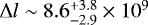 cm for a flare of Proxima in March 2009. In this case the brightness temperature estimates drop to Tb ~ 109 K, which would be compatible with fundamental plasma emission, or even an incoherent emission mechanism, such as (gyro)synchrotron. Thus, while the high circular polarization and sharp spectral cutoff of the flares are clear indicators of emission via the ECM mechanism, the estimates of Tb are highly uncertain and a contribution from (gyro)synchrotron to the non-flaring emission cannot be ruled out. Second harmonic plasma emission can reach higher temperatures, and can more easily account for the observed flux densities. However, the high degree of polarization observed through our observing campaign is hard to reconcile with second harmonic plasma emission. While we cannot rule out that plasma emission contributes to the relatively quiescent level of radio emission observed from Proxima, we have difficulties in using it to explain the observed characteristics at the times of enhanced emission. For example, while second harmonic plasma emission can account for the observed brightness temperatures, the high degree of polarization observed through our observing campaign does not favor this harmonic emission; for example, second harmonic emission in the Sun has shown polarization levels up to about 20%, much less than observed in Proxima.
4.1.2 Electron-cyclotron maser emission from star–planet interaction in Proxima Cen
The other coherent mechanism capable of producing significant radio emission is the electron-cyclotron maser emission (ECM) mechanism, which also yields amplified, highly polarized radiation. In the case of star–planet interaction (or planet–satellite, as in Jupiter–Io), the friction of the planet with the magnetic field of the star generates an unstable population of electrons that gives rise to significant coherent radio emission. This emission is constrained within an anisotropic thin hollow cone, whose axis coincides with the local magnetic field vector (Wu & Lee 1979; Melrose & Dulk 1982), and is visible only when the walls of this cone are aligned with the observer’s line of sight. The ECM mechanism mainly amplifies one of the two magneto-ionic modes (with opposite senses of circular polarization) of the electromagnetic wave propagating within the magnetized plasma (Sharma & Vlahos 1984; Melrose et al. 1984), which explains the high degree of circular polarization of the observed radio emission.
The physical conditions of the region where the ECM efficiently takes place, namely the ambient plasma density and the strength of the local magnetic field, define which dominant magneto-ionic mode is amplified. The helicity of the electrons moving within the stellar magnetosphere univocally define the circular polarization sign of each mode. Hence, regardless of the amplified magneto ionic mode, the ECM arising from the two opposite magnetic hemispheres will be detected as circularly polarized radiation having opposite senses of polarization. As an example, the circular polarization sense of the ECM arising from the early-type magnetic stars carries clear information regarding the stellar hemisphere where the ECM originates (Leto et al. 2016).
In the case of Proxima, the observed radio emission takes place at the expected ECM frequency for the stellar magnetic field intensity of ~600 gauss. The long-term radio emission from Proxima also displays brighter flux densities, stronger variations, and a higher fraction of circular polarization in the low-frequency band (centered at 1.62 GHz), compared to the radio emission in the high-frequency band (centered at 2.52 GHz), in agreement with expectations from ECM emission due to star–planet interaction. We note that our observed 1.62 GHz Stokes I flux density, which ranges from ~174 μJy to ~5.0 mJy during our monitoring campaign of Proxima Cen, broadly agrees with the theoretical flux densities calculated by Turnpenney et al. (2018) for Proxima Cen, who quote values from ~10 μJy up to the mJy level. We also show in Appendix B that theoretical estimates of the Poynting flux arising from star–planet interaction range from as little as 1.4 × 10²⁰ erg s−1 to as much as 4.4 × 10²³ erg s−1. These theoretical estimates are broadly consistent with the Poynting fluxes inferred from our observations (see Figs. B.1 and B.2).
4.1.3 Two maxima of emission per orbital period of Proxima b
Our data indicate the existence of two maxima of emission per orbital cycle (Fig. 5). Two broad emission peaks per orbital period is the expected behavior for the emission from star–planet magnetic interaction of the same sort as the Jupiter–Io interaction, which gives rise to double-peaked auroral radio emission from Jupiter per orbital cycle of Io. We note that any apparent periodicity in our data is unrelated to the rotation of the Proxima Centauri star, which has a rotational period Prot ≈ 83.5 days (Benedict et al. 1998).
The maxima of radio emission fall near the quadratures of the planet Proxima b, also in analogy with the Jupiter–Io interaction where the maxima of radio emission happen around the quadrature positions (Marques et al. 2017). However, since our radio observations span only 1.6 orbital periods, we need to assess the significance of these possible periodic enhancements. To this end, weestimate the likelihood that the observed pattern of radio emission from Proxima Cen has two emission peaks per orbital period, and that these peaks align well with the known physical periodicity by mere chance. The standard way of estimating this likelihood, if the pattern is sinusoidal with a well-defined amplitude, is by means of a Lomb-Scargle periodogram. However, the radio emission does not vary sinusoidally in our case, so we had to revert to a different method. Specifically, we used the minimum string length (MSL) method that, in contrast to other methods used to build periodograms, is suitable for all sorts of light curves (single-peaked or multi-peaked, sinusoidal or non-sinusoidal), and does not require choosing any parameters. The MSL method rests on the fact that the length of a line joining all the points sorted in phase will be small when a correct period is used to derive the phases. In this type of periodogram, potential periods appear as minima in string length plots. However, while the MSL method and other similar techniques are well suited to analyzing periodic signals with smooth behavior, they are not aimed at analyzing periodic signals that can have huge excursions in flux from one cycle to the next. Therefore, we excluded the data corresponding to the huge flare in the last three days of our observing campaign (square symbols in Fig. 5). In this way we smoothed out the large flux density variations observed during our campaign. Therefore, we used 14 of the 17 flux density measurements available.
We therefore computed the string length periodograms (Dworetsky 1983) of 1000 random simulated observing runs (by shuffling themeasured flux densities each time), and compared the simulated MSL of the light curves (folded at 11.2 ± 0.8 days) with the MSL of the observed flux densities within that interval of periods. The above quoted value of ± 0.8 around 11.2 days corresponds to a rough estimate of the uncertainty with which one might determine the value of the period, using a dataset with noise levels and time span such as ours. The MSL in the random tests was equal to or smaller than that of the observations in 51 out of the 1000 simulated runs. The false-alarm probability of the observed configuration of our radio data is thus at most p ≃ (51∕1000) = 0.051, since from avisual inspection of those 51 cases it turns out that about half of the randomly generated light curves had two emission peaks per orbital cycle. Hence, the false-alarm probability of the observed configuration of our radio data is of only p ≃ (26∕1000) = 0.026, and the probability that it did not happen by chance is 1 − p ≃ 0.97. This estimate is a very high value, indicating that it is highly unlikely that the observed data configuration happened by mere chance. If we use the Stokes V measurements instead of Stokes I, we obtain similar results. We also note that the polarized emission also peaks close to the quadratures, as also observed in the Jupiter–Io system.
In summary, the observed properties favor the ECM mechanism over plasma emission as the coherent mechanism responsible for the radio emission from Proxima. In particular, the peaked radio emission close to the quadratures is naturally expected by the ECM mechanism via star–planet interaction, but is hard to reconcile with the plasma emission mechanism. In addition, the two observed broad emission peaks per orbital period, which happen around the quadrature positions of Proxima b, are unlikely to have occurred by mere chance, and is in analogy with the radio behavior observed in the Jupiter–Io system. We therefore suggest that the ECM instability arising from star–planet interaction could be the main physical mechanism responsible for the observed radio emission from Proxima. In this case, the Proxima–Proxima b system would be an analog to the Jupiter–Io system, and a detailed geometrical modeling (Leto et al., in prep.) is able to explain the observed temporal pattern and the reversal of the circular polarization sign of the emission via this ECM mechanism. In the case of ECM triggered by star–planet interaction, the orientation of the magnetic field vector of the stellar magnetosphere univocally defines the sign of the circularly polarized ECM emission. Hence, in addition to the planet position, the stellar magnetosphere orientation also has a crucial role in the capability of detecting planet-induced ECM emission. Coherent ECM emission occurring close to the two quadrature positions of Proxima b might arise from opposite hemispheres of Proxima; the coherent emission corresponding to each of those two positions will be characterized by circular polarization of opposite signs. This is the case of the reversal in the polarization sign of the pulses of the coherent ECM emission observed in the ultra-cool dwarf TVLM513 (Hallinan et al. 2007), whose ECM emission behavior was suggested as an indirect hint of star–planet interaction (Leto et al. 2017).
4.2 Flaring activity of Proxima
The two short flares on April 24, 2017, happened 3.3705 ± 0.0001 days (flare F1) and 3.6313 ± 0.0001 days (flare F2) after JD 2457864.4563, the estimated time of the nearest conjunction of the planet Proxima b (Sect. 3.1), which we adopt as phase reference (ϕ0 = 0). Therefore, the orbital phases of the two short flares relative to this reference are ϕF1− ϕ0 = 0.30131 ± 0.00005 and ϕF2− ϕ0 = 0.32463 ± 0.00005, where uncertainties are calculated by error propagation of the uncertainty on the timing of the peaks of the flares (±10 s) and in the orbital period of the planet (±0.0002 d; Anglada-Escudé et al. 2016). Absolute phases, necessary for a proper comparison with distant events, are largely dominated by the uncertainty on the calculation of the time of the conjunction adopted to set the reference phase ϕ0. The 90% confidence interval of this calculation is [−1.09 d,+0.90 d]. Therefore, the absolute orbital phases of the short flares were 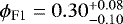 and
and  . Both short-duration flares are consistent with happening close to the first quadrature of the planet (ϕQ1 = 0.25), within the uncertainties. This, together with the high degree of circular polarization, suggests that the short-duration flares in Proxima Cen could be related to a given star–planet orbital position. Two flares were detected during the 10 h on-source of the April 24 session, which means that if these short-duration flares were randomly distributed in orbital phase we should have detected > 1.7 additional flares of similar intensity (90% confidence lower limit assuming small-number Poisson statistics; Gehrels 1986) during the 32 h of total on-source time of the remaining 16 sessions (excluding the April 15 epoch, for which we could not obtain an image in the low-frequency band.) However, we see no evidence in our data of any other flare of similar intensity. If, on the contrary, the occurrence of the short-duration flares were associated with some specific geometrical configuration (e.g., near a quadrature of the planet, such as on April 24) then the appropriate dates would be much more restricted, and the expected number of detected flares would consequently be much smaller, and consistent with the non-detection of additional short-duration flaring activity.
The long-lasting burst at the end of our campaign might suggest that the nature of its radio emission is different from the rest of our data. However, we note that the peak of the burst happens approximately on April 28.8 ± 0.5, 2017 (see Fig. 2 and Table 1), or 7.8 ± 0.5 d after the conjunction of reference where ϕ = 0 is assumed. Taking into account the uncertainties on the timing of the peak, on the orbital period, and on the reference phase, the absolute orbital phase obtained is  , which is close to the second quadrature (ϕQ2 = 0.75). We note that this long burst of emission shows brighter flux densities, stronger variations, and a higher fraction of circular polarization at frequencies ≤2.0 GHz, and takes place at the expected electron-cyclotron frequency for the stellar magnetic field intensity of ~600 gauss. In particular, the emission on April 28, 2017 (Fig. 4), shows a very steep spectral index (α ≲−7.0;Sν ∝ να) at frequencies below ≃2.0 GHz, indicative of non-thermal emission. This emission seems to switch off abruptly above a frequency of ~ 2.0 GHz. The degree of circular polarization is very high in the low-frequency band (|V |∕I ≳ 80%), implying a coherent process. Thus, the characteristics of the long burst are also consistent with the radio emission being due to the ECM mechanism.
4.3 Comparison with previous radio observations of Proxima b
Slee et al. (2003) observed Proxima Cen with ATCA from May 14.2 to May 15.9, 2000, and detected slowly declining radio emission in the 1.38 GHz (22 cm) band. This emission has a number of similarities with the long-lasting burst at the end of our observing campaign: it has a very steep and negative spectral index (α ≃−12) and a degree of circular polarization close to 100%, and it lasted for ~2 days or more. The values of the flux density reported by Slee et al. (2003) are on the order of a few mJy, similar to the peak flux density of the long-lasting burst in our observing campaign. However, these values correspond to a lower frequency and, given the steep and negative spectral index of the emission, they would translate into almost ten times smaller values at the frequency of 1.62 GHz of our observations, down to the level of what we call the quiescent emission (Sect. 3.1) that is present in our observations at epochs far from the quadratures. Therefore, the radio emission observed by Slee et al. (2003) seems instead to correspond to the decaying stage of a flare that could be similar to the burst observed at the end of our observing campaign. Since the flux density decreased as a function of time during the whole interval of the Slee et al. (2003) observations, it must have had a local maximum before the start of these observations, at an orbital phase  . Thus, the orbital phase of the peak of this possible flare is poorly constrained by their observations.
On August 31, 1991, Lim et al. (1996) detected a relatively short-duration flare (a few minutes to a few tens of minutes, peak of ~ 20 mJy) towards Proxima at 20 cm, with a degree of circular polarization close to 100%. The flare happened on August 31.12, 1991, corresponding to an orbital phase  , which is consistent with that flare happening at or around Q2. This flare could have been similar to the short-duration ones we detected on April 24, 2017 (Sect. 3.2).
Finally, at much shorter wavelengths, MacGregor et al. (2018) reported a short-duration (< 1 min) strong 1.3 mm flarepeaking on March 24, 2017, at 08:03 UTC, using ACA observations. In contrast to the centimeter flares, this flare occurred at an orbital phase of  (close to the planet opposition) which is, within the uncertainties, incompatible with a quadrature. Since this flare occurred within a few weeks of our ATCA observing campaign, the relative phasing uncertainty with respect to our flaresis very well constrained to within 0.0004 in phase. We note that while all of the flares observed at centimeter wavelengths can be explained as being powered by the ECM mechanism, the flare observed at 1.3 mm occurred at a wavelength where the ECM, or plasma, coherent mechanisms cannot be powering the observed emission.
In summary, so far five flares have been reported at ~20 cm towards Proxima Cen: three in our data (the two short flares and the long-lasting burst), and those reported by Slee et al. (2003) and Lim et al. (1996) (see Fig. 6). In four of them (excluding the Slee et al. flare) the orbital phase of their peak emission is fairly well constrained and agrees with a quadrature of the planet Proxima b within the uncertainties (90% confidence level) of the orbital parameters. With the current uncertainties, the agreement between the flare peak and a quadrature is constrained within a phase range of 0.18 [+0.08, −0.10] for each of the two short flares, 0.20 [+0.09, −0.11] for the long burst and 0.38 [+0.21, −0.17] for the Lim et al. (1996) flare. Since the probability of the random coincidence of a given flare with a quadrature (either Q1 or Q2) equals the fraction of the phase-space covered by the uncertainties of the two quadratures (twice the above values), the probability of a random coincidence of all four observed flares with a quadrature (either Q1 or Q2) is 0.36 × 0.36 × 0.40 × 0.76 = 0.04. This probability is quite small and suggests a possible relationship between centimeter radio emission and the orbital phase of planet Proxima b. Given the additional properties of the observed emission, this is suggestive of an ECM star–planet interaction, a possibility that deserves further investigation. Monitoring the stellar radial velocities and the radio emission will better characterize the occurrence of both quadratures and radio flares, and can improve our understanding of the Proxima Cen system and its magnetic environment.
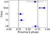 |
Fig. 6 Identified radio flares at centimeter wavelengths (data points) from the Proxima Centauri system against orbital phase of their emission peaks. The dashed vertical lines correspond to the quadrature positions. During our ATCA observationstwo short flares, F1 and F2 (Fig. 2 and Sect. 3.2), and a long-lasting burst, LB (Fig. 2), were observed. The flares labeled “Lim” and “Slee” correspond to the centimeter wavelength flares observed in 1991 and 2000 by Lim et al. (1996) and Slee et al. (2003) (see Sect. 4.3). The error bars indicate the total uncertainties on the phases of the flares, including the contributions due to the uncertainty on the time of the flare peak, on the orbital period, and on the absolute phase reference. The Slee flare peaked before the start of those observations, and only an upper limit to its phase is known. This is indicated by the blue arrow. |
5 Summary
We observed the Proxima system over 18 consecutive days in April 2017 using the Australia Telescope Compact Array (ATCA) at the frequency band of 1.1–3.1 GHz. Our main findings can be summarized as follows:
-
We detected radio emission from Proxima for most of the observing sessions of our radio monitoring campaign, which spanned ~1.6 orbital periods of the planet Proxima b and enclosed four quadrature positions. The emission is stronger at the lower frequency band, around 1.6 GHz, which coincides with the expected electron-cyclotron frequency for the star’s surface magnetic field intensity of ~600 gauss, and exhibits a large degree of circular polarization, which also reverses its sign in the second half of our monitoring campaign.
-
The observed radio emission shows long-term variability with a pattern that is consistent with the orbital period of the planet Proxima b around the star Proxima. Specifically, the 1.6 GHz radio emission presents two emission enhancements per orbital period of Proxima b, occurring at the orbital phase ranges of 0.36 ± 0.09 and 0.81 ± 0.09, i.e., closeto the quadratures. The probability that this observed configuration of the data happened by chance (the false alarm probability) is ~3%.
-
Our observations also show a long burst of radio emission that lasted for about three days, whose emission peak agrees within the uncertainties with the second quadrature of the planet Proxima b. We also detect two short-term flares, few minutes in duration, coincident with the first quadrature within the uncertainties. The observed characteristics of the radio emission in the long- and short-duration flares (frequency around 1.6 GHz, steep and negative spectral index, peak flux densities of a few to a few tens of mJy, degree of polarization close to 100%, and peak near a quadrature) are consistent with being caused by the electron-cyclotron mechanism.
-
There is a clustering of the observed centimeter flares around the quadrature positions, with all known centimeter flares whose peaks have been observed (four since 1991) peaking within uncertainties with a quadrature. While this does not necessarily imply a precise coincidence between flare peaks and quadratures, the probability of all these flares peaking close to the quadratures by mere chance is ~4%, which suggests a relationship between this kind of radio emission and the orbital phase of Proxima b.
-
The ECM emission mechanism accounts well for the observed characteristics of the radio emission, and naturally explains the two emission enhancements observed per orbital cycle of Proxima b, close to the quadrature positions of the planet. While coherent plasma emission may make some contribution to the overall observed radio emission, it shows characteristics that do not match several aspects of our observations, and are hard to reconcile with the observed two enhancements per orbital cycle. The observed radio flux densities are also in broad agreement with theoretical expectations for ECM emission arising from sub-Alfvénic interaction of Proxima Cen with its host planet Proxima b.
In summary, the observed 1.6 GHz radio light curve of Prox- ima Cen shows an emission pattern that is consistent with the orbital period of the planet Proxima b around the star Proxima and with its emission peaks happening near the quadratures. Furthermore, the properties of the observed radio emission (frequency, large degree of circular polarization, change of the sign of circular polarization, and observed level of radio emission) are all consistent with those expected from electron cyclotron-maser emission arising from sub-Alfvénic star–planet interaction. We therefore favor an interpretation of our radio observations in terms of interaction between the star Proxima and its planet Proxima b, which gives rise to the observed radio emission. Under this interpretation, the Proxima-Proxima b system may then represent a scaled-up analog of the observed phenomenology in the Jupiter–Io system or the Jupiter–Ganymede system, where the planet–moon magnetic interaction gives rise to electron-cyclotron radio emission in the decametric spectral region.
The Proxima Cen planetary system, because of its proximity to Earth, is a particularly valuable target to test the possibility of a detectable star–planet interaction. Signs of this possible interaction have been identified in our radio observations thanks to our relatively large monitoring campaign compared to other precedent observations, and to the knowledge of the planet orbital parameters obtained from optical radial velocity (RV) data. It is expected that both the radio and the RV data of Proxima Cen will be significantly improved in the near future, providing a more robust way to establish and characterize this star–planet interaction, if present.
Studying the magnetic interaction of other planets around M-dwarf stars (with intense enough magnetic fields as to emit at decimetric wavelengths), will be possible with future sensitive radio telescopes, such as the SKA (Zarka et al. 2015) or its precursors, and may represent a powerful way of detecting and characterizing exoplanets around stars in the solar neighborhood, and may open a new field of exoplanet–star plasma interaction studies, thus expanding magnetospheric and stellar physics.
Acknowledgements
We thank the anonymous referee for the many useful comments and suggestions, which improved our paper. The Australia Telescope Compact Array is part of the Australia Telescope National Facility which is funded by the Australian Government for operation as a National Facility managed by CSIRO. M.P.-T, J.F.G., J.L.O., G.A., J.L.G., E.R., A.A., P.A., M.O., M.J.L.-G., N.M. and C.R.-L. acknowledge financial support from the State Agency for Research of the Spanish MCIU through the “Center of Excellence Severo Ochoa” award to the Instituto de Astrofísica de Andalucía (SEV-2017-0709). We also acknowledge funding support through the following grants: M.P.-T. and A.A. to PGC2018-098915-B-C21 (FEDER/MCIU-AEI); J.F.G., G.A., M.O. to AYA2017-84390-C2-1-R (FEDER/MCIU-AEI); J.L.O. to AYA2017-89637-R (MINECO) and Junta de Andalucía 2012-FQM-1776; J.L.G. to AYA2016-80889-P (MINECO); E.R, to AYA2016-79425-C03-03-P (MINECO) and ESP2017-87676-C05-02-R; P.J.A. and C.R.L. to AYA2016-79425-C03-03-P; M.J.L.-G. to ESP2017-87143-R (MINECO); and Z.M.B. to CONICYT-FONDECYT/Chile Postdoctorado 3180405.
Appendix A Brightness temperature of the coherent plasma emission
We calculated the brightness temperature, Tb, for the fundamental and harmonic of the coherent plasma emission by following the prescriptions in Stepanov et al. (2001). Namely, we assumed a Langmuir wave spectrum between the wavenumbers kmin = 2πνp∕v1 and kmax = 2πνp∕(5 vth), which takes into account the damping of Langmuir waves at the thermal background, and implies T1 ≳ 25 T (Stepanov et al. 2001). Here, νp is the plasma frequency, which we take equal to 1.62 GHz, ![Mathematical equation: $v_1 = c\, [1 - (m_{\textrm{e}} c^2/(kT_1 + m_{\textrm{e}} c^2))^2]^{1/2}$](/articles/aa/full_html/2021/01/aa39052-20/aa39052-20-eq12.png) is the velocity of the hot electrons, and
is the velocity of the hot electrons, and  is the thermal velocity of the cold, ambient electrons. We used a conservative value of 10−5 for the fraction of kinetic energy density of the ambient plasma that goes into the energy density in Langmuir waves (Dulk 1985). We used a coronal temperature T = 2 × 10⁶ K, as in Appendix B, and estimated the scale height, Ln, by assuming a hydrostatic density structure for the star, so that Ln = k T∕(μ mH g), where μ is the mean atomic weight and g is the star’s gravity. Normalizing to solar values, we obtain
  cm. For the Proxima Cen star, we get Ln ≈ 1.0 × 109 cm ≈ 0.10 R* (R* = 0.145 R⊙ is the radius of the Proxima Cen star). We then varied T1 from 5 × 10⁷ K to 5 × 10⁸ K to calculate the range of brightness temperatures for the fundamental,
  , and the harmonic,
  (Eqs. (15) and (16) in Stepanov et al. 2001).
  varies from 6.4 × 10⁸ K up to 1.0 × 10¹⁰ K, and
  varies from 9.9 × 10¹⁰ K up to 2.4 × 10¹¹ K. Since our observed Stokes I flux densities, F, are in the range from F = 174 μJy to F = 5.0 mJy, the corresponding observed brightness temperatures are
 ![Mathematical equation: $T_{\textrm{b}} \gtrsim (1.0{-} 31)\times10^{10}\,[\Delta l/ (0.1\, R_{\ast})]^{-2}$](/articles/aa/full_html/2021/01/aa39052-20/aa39052-20-eq19.png) K. Therefore, fundamental plasma emission could marginally account for the quiescent level of radio emission detected during our observing campaign, but has difficulties in accounting for the flux density enhancements seen around the quadratures.
K. Therefore, fundamental plasma emission could marginally account for the quiescent level of radio emission detected during our observing campaign, but has difficulties in accounting for the flux density enhancements seen around the quadratures.
Appendix B Radio energetics from star–planet interaction
Here, we discuss the feasibility that the radio emission arising from star–planet interaction in Proxima Cen can be detected in our observations, and follow the formalism of Vedantham et al. (2020).
Theoretical estimates of the Poynting flux due to star–planet interaction in the sub-Alfvénic regime (i.e., when the relative velocity between the stellar wind flow and the planet, vrel, is smaller than the plasma Alfvén velocity, vA) at the location of the planet, are given in Zarka (2007), Lanza (2009), Saur et al. (2013), and Turnpenney et al. (2018), among others. These estimates indicate that the total Poynting flux is  , where Reff is the effective radius of the planetary obstacle, Bsw is the stellar wind magnetic field at the location of the planet, and ϵ ≤ 1 encapsulates efficiency and geometric factors related to the nature of the interaction. We can rewrite the theoretical total Poynting flux as
 (B.1)
(B.1)
where we have normalized the effective radius of the obstacle, Reff, to the radius of Proxima b, which is Rp ≈ 1.1 R⊕ (Bixel & Apai 2017).
The parameter  can be compared with the Poynting flux inferred from the observed radio emission,
  . The total emitted radio power is PR = F Ω D2 Δν, where F is the observed radio flux density, Ω is the solid angle into which the ECM radio emission is beamed, D is the distance to the star, and Δν is the total bandwidth of the ECM emission. We assume a typical bandwidth for the ECM emission of Δν = νg∕2, where νg ≈ 2.8 B* MHz is the cyclotron frequency and B* is the average surface magnetic field strength of the Proxima Cen star. The observationally inferred Poynting flux is thus
  , where the factor ϵrad corresponds to the efficiency in converting the Poynting flux into ECM emission. For D = 1.3 pc, and using an average flux density value at 1.62 GHz of F ≈ 0.31 mJy, the power emitted is PR ≈ 4.2 × 10¹⁹ (F∕300 μJy) (B*∕600G) (Ω∕1 sr) erg s−1, and
  can then be written as
 (B.2)
(B.2)
The efficiencies in the conversion of Poynting flux into ECM emission (the factor ϵrad) are estimated tobe in the range from about 1% (Aschwanden 1990) to values of 10% or even higher (Kuznetsov 2011). Equations (B.1) and (B.2) show that star–planet interactions can potentially result in Poynting fluxes large enough that detection of its centimeter radio emission from Earth is feasible.
We assume that the electrons responsible for the cyclotron emission have kinetic energies between Ek, min =10 keV and the rest-mass of the electron, Ek, max = me c2 = 511 keV. The speed of the electrons, β, depends on the Lorentz γ factor as  , where γ = 1 + Ek∕(me c2). Thus, the above range of kinetic energies corresponds to β in the range [0.20, 0.87]. We make the standard assumption that the electrons emit from within a cone with half-opening angle θ and angular width Δθ, which are related to β as cos θ ≈ Δθ ≈ β (Melrose & Dulk 1982). For our values of Ek, min and Ek, max, the beam solid angle subtended by the emission cone is in the range from 1.20 to 2.6 sr.
We discuss two cases of magnetic field geometry for the star–planet interaction: a close-field dipole geometry and an open-field Parker spiral geometry, also as in Vedantham et al. (2020). For each case we consider two models for the efficiency of the interaction. One model follows the prescriptions by Saur et al. (2013) and Turnpenney et al. (2018), where  . Here MA = vrel∕vA is the Alfvén number at the planet location, Θ is the angle between the stellar wind magnetic field at the planet and the stellar wind velocity in the frame of the planet (e.g., Saur et al. 2013; Turnpenney et al. 2018), and
  is the plasma flow–obstacle interaction strength factor, which for the case of Proxima b is closely approximated by
  (Turnpenney et al. 2018). We followed the prescriptions given in Appendix B of Turnpenney et al. (2018) to determine the speed of the stellar wind, vsw; the magnetic field of the wind, Bsw; and the angle Θ. As in Turnpenney et al. (2018), we used an isothermal stellar wind (Parker 1958), which is fully parameterized by the sound speed or, equivalently, by the coronal temperature T. We adopted T = 2 × 10⁶ K for the coronal temperature of Proxima Cen, which agrees well with the temperatures inferred from X-ray observations(e.g., Fuhrmeister et al. 2011). The other model follows Zarka (2007) and Lanza (2009), where ϵ = η∕2 and η is a geometric factor, which we assume to be η = 1∕2. Since sinΘ ≤ 1 and usually MA ≪ 1, we note that the Zarka-Lanza model predicts significantly larger Poynting fluxes than the Saur-Turnpenney model (see Figs. B.1 and B.2).
We adopted B* = 600 G for the stellar surface magnetic field (Reiners & Basri 2008), which decreases with radial distance as r−3 (closed dipole geometry) and as r−2 (open field geometry). We obtained the effective obstacle radius, Reff(≥ Rp), by balancing the pressure of the planet’s magnetosphere with that of the stellar wind flow. We followed Lanza (2009) and took Reff to be the distance from the planet at which the stellar and planetary magnetic fields are equal, i.e.,  , where Bsw is the magnetic field of the wind at the orbital distance of Proxima b, and Bp the planetary magnetic field. The value of Reff is further modified by a factor of order unity that depends on the angle ΘM between themagnetic moment of the planet and the stellar magnetic field (Saur et al. 2013), which we set equal to ΘM= 0 and ΘM= π∕2 for the closed- and open-field cases, respectively.
We show in Figs. B.1 and B.2 the theoretically expected and observationally inferred range of values for the Poynting flux for our adopted nominal model with ncorona = 107 cm−3, T = 2 × 10⁶ K and a planetary magnetic field of Bp = 1 G. We obtained the plasma density at the orbital distance of Proxima b by letting the value of density evolve at the base of the stellar corona, ncorona, with radial distance as r−2. Figure B.1 corresponds to a Parker spiral (open) geometry of the magnetic field, while Fig. B.2 is for a dipolar (closed) magnetic field geometry. The theoretical expectations for the Poynting flux are drawn as solid lines (blue: Saur/Turnpenney model; green: Zarka/Lanza model), while observationally inferred values are drawn as light orange shaded areas. The orange shaded areas in both figures correspond to the range of observationally inferred Poynting fluxes,  , for our observed Stokes I flux densities (from F = 174 μJy up to F = 5.0 mJy), taking into account the range of beam solid angles of the emission (see above), and the range of the efficiencies in converting Poynting flux into radio emission, ϵrad, which we took to be from 1% up to 10%. For the nominal values of B*, Bp, and ncorona, the theoretically expected Poynting fluxes in the open field case are of
  of 8.7 × 10²⁰ erg s−1 and 4.4 × 10²³ erg s−1 for the Saur/Turnpenney model and the Lanza/Zarka model, respectively (Fig. B.1). In the closed magnetic field case, the expected values of
  are 3.0 × 10²⁰ erg s−1 and 1.4 × 10²⁰ erg s−1 for the Saur/Turnpenney model and the Lanza/Zarka model, respectively (Fig. B.2).
Figure B.3 shows the dependence of the Poynting flux (computed at the orbital distance of Proxima b) on the magnetic field of the planet, Bp, for both magnetic field geometries. We note that, since the magnetic field of the wind at the position of Proxima b is significantly larger in the open-field case than in the closed-field case, the Poynting flux is correspondingly higher. In the open-field case,  is constant for planetary magnetic fields below ~40 mG because for smaller values of Bp, the effective radius of the obstacle, Reff, equals the planet radius Rp. We show in Figs. B.4 and B.5 the dependence of the Alfvén number and Poynting flux on the density at the orbital distance of Proxima b, np. Since rorb∕R* = 71.9, the plasma density at the orbital position of Proxima b is related to the density at the base of the corona as follows:
  . For high densities, the regime becomes supra-Alfvénic, and hence the Poynting fluxes do not apply. We also note that the Poynting flux predicted by the Saur/Turnpenney model increases with density as
  (all other parameters being fixed), while that predicted by the Zarka/Lanza model remains constant. This is because
  in the former (Saur et al. 2013), while
  constant in the latter.
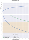 |
Fig. B.1 Comparison of theoretical expectations and observationally inferred values of the Poynting flux from sub-Alfvénic interaction in Proxima, for an open Parker spiral magnetic field geometry, as a function of the radial distance to the Proxima Cen star. Upper panel: Alfvén number, MA. The curves in the lower panel correspond to the theoretical Poynting flux, |


These figures illustrate that the star–planet interaction between the Proxima star and its planet Proxima b is capable of yielding Poynting fluxes that are broadly consistent with the observed radio flux densities.
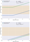 |
Fig. B.3 Comparison of theoretical expectations and observationally inferred values of the Poynting flux from sub-Alfvénic interaction in Proxima as a function of the magnetic field of the planet Proxima b. Top: open magnetic field; bottom: closed magnetic field. |
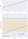 |
Fig. B.4 Comparison of theoretical expectations and observationally inferred values of the Poynting flux from sub-Alfvénic interaction in Proxima as a function of density at the base of the stellar corona, for an open magnetic field geometry. |
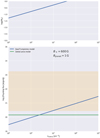 |
Fig. B.5 Same as in Fig. B.4, but for a closed magnetic field. The regime stops being sub-Alfvénic at the orbital distance of Proxima b for ncorona ≈ 3.8 × 107 cm−3, corresponding to a density of about 7000 cm−3 at the orbital position of Proxima b. |
References
- Anglada-Escudé, G., Amado, P. J., Barnes, J., et al. 2016, Nature, 536, 437 [NASA ADS] [CrossRef] [PubMed] [Google Scholar]
- Anglada, G., Amado, P. J., Ortiz, J. L., et al. 2017, ApJ, 850, L6 [NASA ADS] [CrossRef] [Google Scholar]
- Aschwanden, M. J. 1990, A&AS, 85, 1141 [NASA ADS] [Google Scholar]
- Bell, M. E., Lynch, C., Kaplan, D. L., et al. 2016, ATel, 9465 [Google Scholar]
- Benedict, G. F., McArthur, B., Nelan, E., et al. 1998, AJ, 116, 429 [NASA ADS] [CrossRef] [Google Scholar]
- Berger, E., Rutledge, R. E., Phan-Bao, N., et al. 2009, ApJ, 695, 310 [NASA ADS] [CrossRef] [Google Scholar]
- Bixel, A., & Apai, D. 2017, ApJ, 836, L31 [NASA ADS] [CrossRef] [Google Scholar]
- Caswell, J. L. 1998, MNRAS, 297, 215 [NASA ADS] [CrossRef] [Google Scholar]
- Condon, J. J., Cotton, W. D., Greisen, E. W., et al. 1998, AJ, 115, 1693 [NASA ADS] [CrossRef] [Google Scholar]
- Connerney, J. E. P., Kotsiaros, S., Oliversen, R. J., et al. 2018, Geophys. Res. Lett., 45, 2590 [NASA ADS] [CrossRef] [Google Scholar]
- Das, B., Chandra, P., & Wade, G. A. 2018, MNRAS, 474, L61 [NASA ADS] [CrossRef] [Google Scholar]
- Das, B., Chandra, P., Shultz, M. E., et al. 2019a, ApJ, 877, 123 [CrossRef] [Google Scholar]
- Das, B., Chandra, P., Shultz, M. E., et al. 2019b, MNRAS, 489, L102 [CrossRef] [Google Scholar]
- Dulk, G. A. 1985, ARA&A, 23, 169 [NASA ADS] [CrossRef] [Google Scholar]
- Dworetsky, M. M. 1983, MNRAS, 203, 917 [NASA ADS] [Google Scholar]
- Fuhrmeister, B., Lalitha, S., Poppenhaeger, K., et al. 2011, A&A, 534, A133 [NASA ADS] [CrossRef] [EDP Sciences] [Google Scholar]
- Gehrels, N. 1986, ApJ, 303, 336 [NASA ADS] [CrossRef] [Google Scholar]
- Hallinan, G., Bourke, S., Lane, C., et al. 2007, ApJ, 663, L25 [NASA ADS] [CrossRef] [Google Scholar]
- Kao, M. M., Hallinan, G., Pineda, J. S., et al. 2016, ApJ, 818, 24 [NASA ADS] [CrossRef] [Google Scholar]
- Katarzyński, K., Gawroński, M., & Goździewski, K. 2016, MNRAS, 461, 929 [CrossRef] [Google Scholar]
- Kuznetsov, A. A. 2011, A&A, 526, A161 [NASA ADS] [CrossRef] [EDP Sciences] [Google Scholar]
- Lanza, A. F. 2009, A&A, 505, 339 [NASA ADS] [CrossRef] [EDP Sciences] [Google Scholar]
- Leto, P., Trigilio, C., Buemi, C. S., et al. 2016, MNRAS, 459, 1159 [NASA ADS] [CrossRef] [Google Scholar]
- Leto, P., Trigilio, C., Buemi, C. S., et al. 2017, MNRAS, 469, 1949 [NASA ADS] [CrossRef] [Google Scholar]
- Leto, P., Trigilio, C., Oskinova, L. M., et al. 2019, MNRAS, 482, L4 [NASA ADS] [CrossRef] [Google Scholar]
- Leto, P., Trigilio, C., Leone, F., et al. 2020, MNRAS, 493, 4657 [CrossRef] [Google Scholar]
- Lim, J., White, S. M., & Slee, O. B. 1996, ApJ, 460, 976 [CrossRef] [Google Scholar]
- López Fuentes, M. C., Klimchuk, J. A., & Démoulin, P. 2006, ApJ, 639, 459 [NASA ADS] [CrossRef] [Google Scholar]
- MacGregor, M. A., Weinberger, A. J., Wilner, D. J., et al. 2018, ApJ, 855, L2 [NASA ADS] [CrossRef] [Google Scholar]
- Marques, M. S., Zarka, P., Echer, E., et al. 2017, A&A, 604, A17 [NASA ADS] [CrossRef] [EDP Sciences] [Google Scholar]
- McMullin, J. P., Waters, B., Schiebel, D., et al. 2007, Astronomical Data Analysis Software and Systems XVI (USA: ASP Books), 127 [Google Scholar]
- Melrose, D. B., & Dulk, G. A. 1982, ApJ, 259, 844 [NASA ADS] [CrossRef] [Google Scholar]
- Melrose, D. B., Hewitt, R. G., & Dulk, G. A. 1984, J. Geophys. Res., 89, 897 [NASA ADS] [CrossRef] [Google Scholar]
- Parker, E. N. 1958, ApJ, 128, 664 [Google Scholar]
- Peres, G., Orlando, S., & Reale, F. 2004, ApJ, 612, 472 [NASA ADS] [CrossRef] [Google Scholar]
- Reiners, A., & Basri, G. 2008, A&A, 489, L45 [NASA ADS] [CrossRef] [EDP Sciences] [Google Scholar]
- Route, M., & Wolszczan, A. 2012, ApJ, 747, L22 [NASA ADS] [CrossRef] [Google Scholar]
- Sault, R. J., Teuben, P. J., & Wright, M. C. H. 1995, Astronomical Data Analysis Software and Systems IV (USA: ASP Books), 433 [Google Scholar]
- Saur, J., Grambusch, T., Duling, S., et al. 2013, A&A, 552, A119 [NASA ADS] [CrossRef] [EDP Sciences] [Google Scholar]
- Sharma, R. R., & Vlahos, L. 1984, ApJ, 280, 405 [NASA ADS] [CrossRef] [Google Scholar]
- Slee, O. B., Willes, A. J., & Robinson, R. D. 2003, PASA, 20, 257 [NASA ADS] [CrossRef] [Google Scholar]
- Stepanov, A. V., Kliem, B., Zaitsev, V. V., et al. 2001, A&A, 374, 1072 [NASA ADS] [CrossRef] [EDP Sciences] [Google Scholar]
- Trigilio, C., Leto, P., Leone, F., et al. 2000, A&A, 362, 281 [Google Scholar]
- Turnpenney, S., Nichols, J. D., Wynn, G. A., et al. 2018, ApJ, 854, 72 [CrossRef] [Google Scholar]
- Vedantham, H. K., Callingham, J. R., Shimwell, T. W., et al. 2020, Nat. Astron., 4, 577 [CrossRef] [Google Scholar]
- Wu, C. S., & Lee, L. C. 1979, ApJ, 230, 621 [NASA ADS] [CrossRef] [Google Scholar]
- Zarka, P. 2007, Planet. Space Sci., 55, 598 [NASA ADS] [CrossRef] [Google Scholar]
- Zarka, P., Farges, T., Ryabov, B. P., et al. 1996, Geophys. Res. Lett., 23, 125 [NASA ADS] [CrossRef] [Google Scholar]
- Zarka, P., Lazio, J., & Hallinan, G. 2015, Advancing Astrophysics with the Square Kilometre Array (USA: SKA), 120 [CrossRef] [Google Scholar]
- Zic, A., Stewart, A., Lenc, E., et al. 2019, MNRAS, 488, 559 [NASA ADS] [CrossRef] [Google Scholar]
All Tables
All Figures
|
Fig. 1 Contour maps of radio continuum emission from the Proxima Centauri system on April 24, 2017. The maps correspond to total (Stokes I) and circularly polarized (Stokes V) flux density, for two bands: 400 MHz centered at 1.62 GHz, and 1 GHz centered at 2.52 GHz. Contour levels are drawn at −2, 2, 4, 6, 8, 10, 12, 14, and 16 times the rms of each map (denoted by σ in each panel). The sign of the Stokes V maps was inverted for better visualization, so solid contours in the two bottom panels actually represent negative values of the circularly polarized flux density. The hatched ellipse in the bottom right corner of each panel represents the half-power contour of the synthesized beams. The cross corresponds to the position of the star Proxima for the observing epoch, obtained from the 1.3 mm ALMA data reported in Anglada et al. (2017), taking into account the proper motion and parallax of the star. |
| In the text | |
|
Fig. 2 Time evolution of flux density in Proxima. Variation of total (Stokes I; panels a and b) and circularly polarized (Stokes V; panels c and d) flux density as a function of time during our ATCA observing campaign. For each observing session the data is averaged over a bandwidth of 400 MHz and 1 GHz centered at 1.62 GHz [wavelength ≃ 18.5 cm; (b,d)] and 2.52 GHz [≃ 11.9 cm; (a,c)], respectively. Vertical lines indicate 1σ uncertainties for each data point, and blue shaded rectangles are 3σ upper limits for non-detections (in the case of Stokes V, they correspond to upper limits to the absolute value of the flux density). The duration of the observation on April 24, 2017 (12 h), is represented with a horizonal blue bar, while the observing time of the other days (~2 h) is smaller than the symbol size of data points. Dashed orange lines show the quadratures, Q1 and Q2, of Proxima b, with the horizontal orange bars indicating the statistical uncertainty on the determination of the epoch of the quadratures (see text fordetails). The horizontal dashed line in the plot of Stokes I at 1.62 GHz (b) corresponds to a flux density of 0.174 ± 0.038 mJy, obtained by averaging together the data over the five observing sessions where the source was not detected individuallyat that frequency. No map could be obtained at low frequency on April 15, 2017, due to an insufficient number of unflagged visibilities. Panels e and f: variation of Stokes I during April 24, 2017, for data averaged over 20 s intervals. Two short-duration flares are evident at 1.62 GHz (f). Panels g and h: temporal close-up of the two flares. The black and red lines correspond to Stokes I and V, respectively. The sign of Stokes V has been reversed for better visualization. |
| In the text | |
|
Fig. 3 Contour maps of Proxima at 1.62 GHz during maximum and minimum emission. Top panel: emission on April 28, 2017, when the flux density was at its maximum. Contour levels are drawn at −6, −3, 3, 6, 12, 24, and 48 × 78 μJy beam−1, the rms of the map. Bottom panel: map obtained by combining the uv data for the observing epochs when the emission was not detected in each of the individual images (April 16, 20, 22, 23, and 26, 2017). Contour levels are drawn at −2, 2, and 4 × 38 μJy beam−1, the rms of the map. In both maps the solid and dotted contours represent positive and negative levels, respectively. |
| In the text | |
|
Fig. 4 Illustration of the day-to-day radio spectral evolution of Proxima. Data correspond to the total flux density (Stokes I) on April 18 (circles), April 24 (squares), and April 28 (diamonds) over the whole observing bandwidth, averaged every 200 MHz. For comparison, we also show the result of stacking the data corresponding to the five individual observing epochs where there was no detection (data of April 16, 20, 22, 23, and 26), drawn as stars. Arrows indicate 3σ upper limits. |
| In the text | |
|
Fig. 5 Flux density light curve of Proxima (1.62 GHz) folded to the orbital period of the planet Proxima b, covering ~1.6 orbital periods. Variation of the total flux density (Stokes I) as a function of the orbital phase of Proxima b (Porb =11.186 days; Anglada-Escudé et al. 2016). The conjunction time, corresponding to the value 0.0 of the orbital phase, is determined to be April 20, 22:57 UTC, with a 90% confidence interval of [+21.7, −26.1] h. The last three days of observations (April 27, 28, and 29; square symbols) correspond to a significantly brighter emission burst, and have been analyzed separately. The 1.62 GHz flux density values are higher in two well-defined regions of the orbital cycle of Proxima b. The centroids of these regions correspond to orbital phases of 0.36 and 0.81 (excluding the data from the brighter burst), and the hatched regions represent the rms width of the maxima of emission. The yellow shaded areas correspond to the 90% confidence interval around the first and second quadratures. The filled and open symbols in panel b correspond to positive and negative values of Stokes V, respectively. The error bars correspond to 1σ uncertainties. |
| In the text | |
|
Fig. 6 Identified radio flares at centimeter wavelengths (data points) from the Proxima Centauri system against orbital phase of their emission peaks. The dashed vertical lines correspond to the quadrature positions. During our ATCA observationstwo short flares, F1 and F2 (Fig. 2 and Sect. 3.2), and a long-lasting burst, LB (Fig. 2), were observed. The flares labeled “Lim” and “Slee” correspond to the centimeter wavelength flares observed in 1991 and 2000 by Lim et al. (1996) and Slee et al. (2003) (see Sect. 4.3). The error bars indicate the total uncertainties on the phases of the flares, including the contributions due to the uncertainty on the time of the flare peak, on the orbital period, and on the absolute phase reference. The Slee flare peaked before the start of those observations, and only an upper limit to its phase is known. This is indicated by the blue arrow. |
| In the text | |
|
Fig. B.1 Comparison of theoretical expectations and observationally inferred values of the Poynting flux from sub-Alfvénic interaction in Proxima, for an open Parker spiral magnetic field geometry, as a function of the radial distance to the Proxima Cen star. Upper panel: Alfvén number, MA. The curves in the lower panel correspond to the theoretical Poynting flux, |
| In the text | |
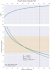 |
Fig. B.2 Same as in Fig. B.2, but for a closed dipolar geometry. |
| In the text | |
|
Fig. B.3 Comparison of theoretical expectations and observationally inferred values of the Poynting flux from sub-Alfvénic interaction in Proxima as a function of the magnetic field of the planet Proxima b. Top: open magnetic field; bottom: closed magnetic field. |
| In the text | |
|
Fig. B.4 Comparison of theoretical expectations and observationally inferred values of the Poynting flux from sub-Alfvénic interaction in Proxima as a function of density at the base of the stellar corona, for an open magnetic field geometry. |
| In the text | |
|
Fig. B.5 Same as in Fig. B.4, but for a closed magnetic field. The regime stops being sub-Alfvénic at the orbital distance of Proxima b for ncorona ≈ 3.8 × 107 cm−3, corresponding to a density of about 7000 cm−3 at the orbital position of Proxima b. |
| In the text | |
Current usage metrics show cumulative count of Article Views (full-text article views including HTML views, PDF and ePub downloads, according to the available data) and Abstracts Views on Vision4Press platform.
Data correspond to usage on the plateform after 2015. The current usage metrics is available 48-96 hours after online publication and is updated daily on week days.
Initial download of the metrics may take a while.