| Issue |
A&A
Volume 644, December 2020
|
|
|---|---|---|
| Article Number | A103 | |
| Number of page(s) | 10 | |
| Section | The Sun and the Heliosphere | |
| DOI | https://doi.org/10.1051/0004-6361/202039108 | |
| Published online | 08 December 2020 | |
Solar east-west flow correlations that persist for months at low latitudes are dominated by active region inflows
1
Center for Space Science, NYUAD Institute, New York University, Abu Dhabi, Abu Dhabi, UAE
e-mail: This email address is being protected from spambots. You need JavaScript enabled to view it.
2
Max-Planck-Institut für Sonnensystemforschung, Justus-von-Liebig-Weg 3, 37077 Göttingen, Germany
3
Institut für Astrophysik, Georg-August-Universität Göttingen, Friedrich-Hund-Platz 1, 37077 Göttingen, Germany
4
Department of Physics, Courant Institute of Mathematical Sciences, Tandon School of Engineering, New York University, New York, 10003 New York, USA
Received:
5
August
2020
Accepted:
22
October
2020
Abstract
Context. Giant-cell convection is believed to be an important component of solar dynamics. For example, it is expected to play a crucial role in maintaining the Sun’s differential rotation.
Aims. We reexamine early reports of giant convective cells detected using a correlation analysis of Dopplergrams. We extend this analysis using 19 years of space- and ground-based observations of near-surface horizontal flows.
Methods. Flow maps are derived through the local correlation tracking of granules and helioseismic ring-diagram analysis. We compute temporal auto-correlation functions of the east-west flows at fixed latitude.
Results. Correlations in the east-west velocity can be clearly seen up to five rotation periods. The signal consists of features with longitudinal wavenumbers up to m = 9 at low latitudes. Comparison with magnetic images indicates that these flow features are associated with magnetic activity. The signal is not seen above the noise level during solar minimum.
Conclusions. Our results show that the long-term correlations in east-west flows at low latitudes are predominantly due to inflows into active regions and not to giant convective cells.
Key words: Sun: helioseismology / Sun: oscillations / Sun: interior / Sun: activity / waves / convection
© ESO 2020
1. Introduction
The transport of heat from the solar interior to the surface is achieved through convective motions in the outer 30% of the Sun. From observations, we currently know of two well-defined scales of convection: granulation and supergranulation. Granulation cells have lifetimes of ∼10 min, have scales of 1–2 Mm (spherical harmonic degree ℓ ≥ 1000), and are well reproduced by numerical studies (see review by Nordlund et al. 2009). Supergranulation is a larger scale of convection at ∼30 Mm (ℓ∼120), with lifetimes of one to two days and a depth structure that is debated (see Rincon & Rieutord 2018, for a review). The nature of convective motions at larger scales (ℓ< 100) is not well understood, with a number of studies reporting different amplitudes (see review by Hanasoge et al. 2016) and different geometries (Beck et al. 1998; Hathaway et al. 2013). Here, we reexamine the earliest reported detection of giant convective cells by Beck et al. (1998), who used a 16-month time series of Dopplergrams from space, by utilizing the subsequent two decades of observations.
In examining surface Doppler images from the Mount Wilson Observatory, Labonte et al. (1981), and later Snodgrass & Howard (1984), concluded that there was no giant cell signal above 1–10 m s−1 per wavenumber. It was not until the availability of data from the Michelson Doppler Imager (MDI) on board the Solar and Heliospheric Observatory spacecraft that Beck et al. (1998) detected long-lived large-scale velocity features. These features were found to have an e-folding lifetime of 126 days and to be highly elongated in longitude (up to 44°), with an aspect ratio > 4 on the surface. Beck et al. (1998) attributed this signal to the presence of giant convective cells. This result has been in contradiction with many numerical studies, which suggest that large-scale convection should form “banana cells” that are elongated in latitude (e.g., Miesch et al. 2008). Ulrich (2001) disputed the convective nature of the observed east-west flow correlations and proposed that they are Rossby or inertial waves.
Recent studies based on granulation tracking, supergranulation tracking, or local helioseismology have identified several components of near-surface large-scale motions: (1) surface inflows into active regions (Gizon et al. 2001; Gizon 2004; Haber et al. 2004); (2) vortical motions due to equatorial Rossby waves below ∼30° latitude with longitudinal wavenumbers m < 15 (Löptien et al. 2018; Hanasoge & Mandal 2019; Liang et al. 2019; Proxauf et al. 2020; Hanson et al. 2020); and (3) east-west velocity features with m = 1 above 50° latitude (Hathaway et al. 2013; Bogart et al. 2015; Hathaway & Upton 2020).
While the aforementioned studies focused on imaging distinct patterns of motion, a number of other studies have focused on constraining the amplitude of the flows. Hanasoge et al. (2012) used local helioseismic techniques to measure the horizontal flow velocities at a depth of 0.96 R⊙, finding upper limits on the amplitudes on the order of 0.1 m s−1 per mode. This suppression of power at large scales compared to numerical simulations is puzzling (see Gizon & Birch 2012, for a commentary), considering that numerical studies had anticipated amplitudes two orders of magnitudes larger (Miesch et al. 2008). Further complicating the debate, Greer et al. (2015) used a different local helioseismic technique and reported amplitudes larger than numerical studies for large-scale features (ℓ < 30), but comparable amplitudes at smaller scales (ℓ > 30). A careful assessment of the issues involved in these studies is available in Proxauf (2020).
In this study, we will address the observations of Beck et al. (1998). With an additional 19 years of observations (spanning nearly two solar cycles, see Fig. 1), we sought to differentiate signals associated with magnetic activity from those associated with non-magnetic processes (Rossby waves and possibly thermal convection). We find that the signals identified by Beck et al. (1998) are very likely due to the active region inflows, even near solar minimum.
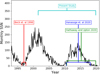 |
Fig. 1. Monthly sunspot number (SSN) for cycles 23 and 24. The observation period of the present study and references herein are highlighted for reference. |
2. Data analysis and results
We used the horizontal flow maps derived from observations of the ground-based Global Oscillation Network Group (GONG, Harvey et al. 1996) and the space-based Helioseismic and Magnetic Imager (HMI, Schou et al. 2012). From the former, we utilized 19 years of horizontal flows derived from the GONG++ ring-diagram analysis (RDA) pipeline from 2001–20201. From the latter instrument, we used eight years of RDA data from 2010–20182 and six years (2010–2016) of surface horizontal flow data derived from the local correlation tracking (LCT) of granules by Löptien et al. (2018)3. For both RDA data sets, we used the flows derived from 15° tiles. To remove small-scale features from the LCT maps, we smoothed them by convolving with a Gaussian of σ = 7.2°.
In total, we have three independent data sets. Corbard et al. (2003) details the GONG++ RDA pipeline, Bogart et al. (2011a,b) details the HMI RDA pipeline, and details of the LCT method are found in Welsch et al. (2004) and Fisher & Fisher & Welsch (2008). For each of these data sets, we have both of the horizontal flow components: in the direction of rotation ux and in the direction of the solar north pole uy. We corrected for center-to-limb effects through the method described by Liang et al. (2019). For clarity in terminology, we refer to ux or uy as the measured flow within a single tile, and east-west (EW) or north-south (NS) as the flow signals averaged over longitude or temporal windows.
2.1. Coordinate system
We examine the flows in the Stonyhurst coordinate system, whereby the frame is rotating at the Earth’s orbital frequency. In this system, the latitude λ and longitude ϕ are zero at the intersection of the equator and the central meridian on the visible disk. The latitude increases in the direction of the solar north pole, while the longitude increases in the direction of solar rotation. Accordingly, the longitudinal flows uϕ are positive if in the direction of rotation, and the latitudinal flows uλ are positive if in the direction of the north pole. The flow components are computed from small patches on the solar disk, assuming a Cartesian geometry (x, y). As such, the approximations ux = uϕ and uy = uλ are taken within each small patch. In this study, we also analyze the horizontal divergence ∇h ⋅ u in spherical geometry, where ∇h = (r cos λ)−1(∂λ cos λ, ∂ϕ) and u = (uλ, uϕ).
2.2. Auto-correlation functions
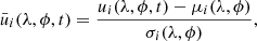
Following Beck et al. (1998), we computed the auto-correlation functions of the flow maps. For each time segment of duration Nt = 720 days, we considered the centered and normalized velocity components
 (1)
(1)
where μi(λ, ϕ) is mean value of ui over the 720-day window and σi(λ, ϕ) is standard deviation. The longitude-averaged auto-correlation of the time series  at fixed latitude at time lag τ is
 (2)
(2)
The auto-correlation of  is
is
 (3)
(3)
Long-lived features will appear as peaks in the auto-correlation at integer values of the local rotation period. The auto-correlations were computed using a temporal window of ∼720 days. Due to the different cadence of each of the data sets, this results in Nt = 633 for each window in the RDA data and Nt = 720 for the LCT data. For each consecutive sample, the window was shifted by Nt/2. In order to improve the signal-to-noise ratio, we then took the mean across longitude and temporal samples. When comparing LCT and RDA, we used the RDA auto-correlation for flows at a depth of ∼2 Mm, which is the shallowest depth from the GONG++ full disk flow map pipeline4. Comparison between HMI RDA and LCT is possible at the surface, though Proxauf et al. (2020) notes that HMI RDA surface measurements are unreliable. The HMI RDA flow inversions that target the surface appear to have excess power at low m, relative to inversions targeting 696 km deeper, and this results in large-scale artifacts in the surface flow maps (Bastian Proxauf, priv. comm.).
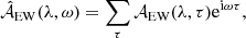
Figure 2 shows the auto-correlations of the EW flows as a function of time lag and latitude. These results are consistent with Beck et al. (1998), showing a long-lived EW flow signal that persists for at least five solar rotations and can be seen at latitudes up to 45°. Due to the latitudinal differential rotation, the peaks in 𝒜 are at greater time lags at higher latitudes. In each data set, the peak in 𝒜 is preceded and followed in time by negative correlation sidelobes.
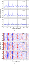 |
Fig. 2. Top: temporal auto-correlation function of the EW flows at the equator for HMI RDA, LCT, and GONG++ RDA. A signal is seen to persist for at least five solar rotations. Statistical error bars are comparable to line thickness and hence are not shown. Bottom: 2D map of the EW auto-correlation maps as a function of latitude and time lag. The deflection with latitude is qualitatively consistent with differential rotation. The dashed vertical lines in each image indicate multiples of the equatorial rotation period. |
Figure A.2 shows similar results for the NS flow signal. However, in order to obtain such clear results, the solar Rossby waves (Löptien et al. 2018) were filtered out (see Appendix A). While similar to the EW signal, the NS signal seems to become consistent with noise within four rotations.
2.3. Spectral analysis
Here, we examine the spectral components of the EW auto-correlation in a similar manner to Ulrich (2001). For this section, we present the results for HMI RDA. The results of the other data sets are similar.
We performed a temporal Fourier transform on the EW auto-correlation function (Eq. (2)),
 (4)
(4)
where the sum is taken over all time lags τ and ω is the angular frequency. In the Stoneyhurst frame, a flow pattern proportional to eimϕ, which is rotating at the rotation rate Ωλ, will have a frequency mΩλ, where Ωλ is the local rotation rate at latitude λ. We have corrected the data for the Earth’s orbital frequency, 31.7 nHz.
Figure 3 shows  as a function of frequency and latitude, at a depth of 2 Mm. These results show that 𝒜EW has components up to m = 9, after which the signal is consistent with noise. At higher latitudes (λ > 40°), modes on the order of m > 6 are not seen. The mode m = 2 at the equator has the greatest amplitude. In the frequency domain, the deflections with latitude seen in Fig. 2 are toward lower frequencies and are qualitatively consistent with differential rotation.
 |
Fig. 3. Plot of |

2.4. Mode parameters of the EW signal
In this section, we characterize the modes that contribute to the long-lived EW signal. We computed the power spectrum P(λ, ω) of the EW flow maps for the entire HMI observation time
 (5)
(5)
where the sum over ϕ is over the range −45° ≤ϕ ≤ 45° for each snapshot. The resulting spectra are similar to Fig. 3 but have an exponential probability distribution function. The azimuthal modes m at each latitude λ were fit assuming a Lorentzian line profile,
 (6)
(6)
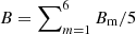
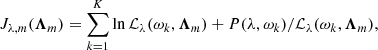
where Am is the mode amplitude, ωm is the mode frequency, Γm is the full width at half maximum, Bm is the background noise of the spectrum, and Λm = {Am, ωm, Γm, Bm}. We fit only up to m = 6 due to poor a signal-to-noise ratio for higher modes. Details of the fitting can be found in Appendix B. We opted to fit each individual mode m using a frequency window of width Δω/Ωλ = 1.
Having fit the power spectrum of the EW flows, we compared the rotational frequencies to those derived from Doppler and magnetic features (Snodgrass & Ulrich 1990). Snodgrass & Ulrich (1990) identified magnetic features from rebinned Mount Wilson magnetograms, with each bin covering approximately 6° in latitude. This coarse grid smooths out small-scale activity and should be dominated by strong magnetic features. As such, the derived rotation rates are consistent with sunspot rotation rates below 40° latitude (see review in Beck 2000). Figure 4 compares these rotation rates to the fit rotation frequencies of the HMI RDA EW power spectrum. These results show a mismatch between the frequencies of the EW signal and Doppler features (supergranules). However, when compared to the magnetic tracers, the EW frequencies are similar at all latitudes. This indicates that the EW flow rotation rate is consistent with the rotation rate of magnetic regions. These results are also in agreement with the HMI LCT and GONG++ RDA data sets.
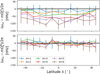 |
Fig. 4. Difference between the rotational frequencies of the long-lived EW signals in HMI RDA and the synodic frequencies of Doppler features ( |


Figure 5 shows the other fit parameters of the HMI RDA EW spectrum. The measured lifetimes (2/Γm) show that, within error estimates, the modes at all latitudes have a lifetime of 4–5 months. This is consistent with Beck et al. (1998). In the HMI RDA flow maps, the signal-to-noise ratio S/N (Am/Bm) is near or above parity (up to six) for modes from m = 2 up to m = 5. Finally, we compared the mean background power 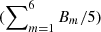 in the three data sets and find values of ∼1–1.2 m s−1, with the greatest power at the active latitudes. This gives a limit on the sensitivity of detecting giant flow cells.
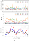 |
Fig. 5. Top: lifetime of the modes seen in the HMI RDA EW power spectrum. Middle: signal-to-noise ratio (Am/Bm). Bottom: background power |
2.5. Relation to activity
The results in the previous sections confirmed the presence of long-lived signals in the near-surface horizontal flows in three independent data sets. However, these results do not confirm the convective or magnetic nature of such flows. Rossby waves rotate retrogradely at fractional values of ω/Ωeq (in the Stoneyhurst frame) and hence can be filtered from the data (see Appendix A). At such large scales and long lifetimes, there remain a few potential causes for the origin of these signals: giant-cell convection, active region inflows, or a side effect of magnetic activity. With the long observation window of GONG++, we will exploit the data of two solar cycles to shed light on the nature of these flows.
To investigate this, we first performed further processing on the flow data sets and filtered out modes greater than ω/Ωλ = 8 and less than ω/Ωλ = 1. This was done with a filter that has a flat top from ω/Ωλ = 1 to ω/Ωλ = 8 and is tapered to zero by a cosine bell that goes from 1 to zero in a distance Δω/Ωλ = 1. This filter was applied to both negative and positive frequencies, and the flow maps were then reconstructed into the time domain. Applying such a filter to the data introduces some smoothing and removes frequencies lower than the equatorial rotation frequency.
For comparison with magnetic activity, we tracked MDI and HMI magnetograms, which overlap with the GONG++ data presented here. We utilized the tracking routine mTrack5, which is the same routine used to track Doppler images for the HMI RDA pipeline. The magnetograms were sampled at a cadence of 96 min. and tracked for 1/24th of a Carrington rotation (CR), which results in 17 magnetograms per data cube. Each magnetogram was projected onto a cylindrical equidistant map, tracked at the Snodgrass magnetic tracer rotation rate (Snodgrass & Ulrich 1990), and subsampled to a resolution of 0.6° per pixel.
The flow and magnetic maps were collected into data cubes spanning one year in time. We then identified converging flow features with amplitudes −∇h ⋅ u > 3 × 10⁻⁸ s−1, considering these signals to be above the background noise in the GONG++ divergence data. Here, we focused on the convergent features since the analysis of the resulting maps is intuitive when considering magnetic activity. We performed the same analysis on EW and divergent flows, finding similar results. At fixed time, among the converging flow features that are within 30° of one another, we selected the largest amplitude feature to avoid counting a large converging flow feature multiple times. Additionally, features outside of 40° from disk center were rejected to avoid the disk-edge. On average, we identified 850 features within each one-year window. For each identified feature, the flow and magnetic maps were shifted such that the feature is positioned at image center. A mean of the images was then computed. In order to determine the evolution of these flows, this procedure was repeated at integer (up to 3) CRs before and after the initial identification. Differential rotation  was accounted for in this averaging routine.
Figures 6 and 7 show these stacked maps for the solar maximum of cycle 23 and the minimum between cycles 23 and 24, respectively. For better visualization, we linearly interpolated the RDA flow maps to improve resolution by a factor of four. In both figures, large-scale flows can be observed at the initial identification time (CR = 0). During the maximum, the EW and NS flows extend 30° (from center) in the longitude direction and 15° in latitude. These flow patterns are seen at least 3 CR before and after initial identification. The computed spatial correlation coefficients show that the flows have a correlation of ∼0.45 with the initial identified features at +3 CR. The corresponding magnetic maps show that these flows are related to activity. We have not included the vorticity here as the Rossby waves and Rossby filters make it difficult to obtain a clean signal at higher latitudes (see Appendix A for a discussion).
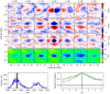 |
Fig. 6. Top panels: average flows around convergent features during the solar maximum of cycle 23. Each of the first three rows is a different component of the flow, from top to bottom: EW flows, NS flows, and divergence maps. The fourth row is the average unsigned magnetic field. Each column is the mean map at an integer rotation before and after the initial identification (0 CR, middle column). Bottom-left panel: monthly sunspot number as a function of year (blue), with the center of the one-year observation window overplotted (vertical black line) and window size shown (shaded gray region). Bottom-right panel: spatial correlation coefficient between the CR = 0 flow maps and the flow maps at time lag CR (EW: blue; NS: orange; ∇h ⋅ u: green). |
During the minimum, the identified flows extend approximately 15° from the center. The associated magnetic maps show very weak magnetic fields. Unlike the maximum, the identified flows in the minimum do not persist beyond a local rotation period. This is further evidenced in the correlation coefficients, which drop to near zero by ±1 CR. The maps of the flows at integer rotations share no visual correlations with the identified feature.
Figure 8 shows the spatial correlation of the flow maps as a function of CR and time. These results further demonstrate that these large-scale flows persist for a number of rotations during solar maximum. As the solar cycle begins its descending phase, the flows persist for shorter periods of time. At the solar minima, 2008 and 2019, the flows persist for no more than one rotation.
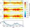 |
Fig. 8. Spatial correlation coefficient between flow maps at CR = 0 and those at time lag CR, as a function of time and CR. The coefficients for the EW, NS, and divergence are shown in the top three panels, with the monthly sunspot number shown for reference in the bottom panel. The large-scale flows persist for a number of rotations during periods of high solar activity. |
3. Discussion and conclusions
We have investigated the long-lived large-scale EW flow signal reported by Beck et al. (1998). Using nearly 20 years of flow maps derived from observations by both GONG and HMI, we confirm the presence of this signal in the near-surface horizontal flows. However, with careful comparisons with magnetic field maps, we find that these signals are consistent with magnetic active region inflows. Specifically, the rotation rate of these signals is consistent with the measured rotation rate of magnetic features (Snodgrass & Ulrich 1990). Furthermore, we find that there are no long-lived features, above the noise level, observed to persist beyond a rotation during the solar minimum.
Beck et al. (1998) observed giant long-lived velocity features and attributed these features to convection. This conclusion was based on the assumption that their data set, consisting of MDI Dopplergrams from 1996 to 1997, would not be significantly contaminated by magnetic activity during a minimum. While active region inflows were not discovered at this time, the authors were still aware that magnetic activity would affect the results. Nevertheless, during this observation window, cycle 23 was ascending and the monthly sunspot number was growing from 10 to 45 (see Fig. 1). We investigated a similar period in cycle 24 (2009, one year after Fig. 7) and found inflows into active regions that persisted for a number of months. These inflows are at a weaker level than in Fig. 6 and, after three rotations, have a spatial correlation coefficient of 0.25. The EW component of these inflows is what is observed in the correlation functions of Beck et al. (1998). We note that there is a very small window (one year centered at the minimum) in which inflows do not dominate the low-latitude flow field. Interestingly, the studies of Labonte et al. (1981) and Snodgrass & Howard (1984) did not report on these long-time correlations, despite the data covering cycles 20 and 21 and the supposed sensitivity of ∼1 m s−1 per wavenumber.
The reported observations from Beck et al. (1998) are consistent with ours, with the exception that they incorrectly identified the large velocity cells as convective in origin. Specifically, the EW correlations have an e-folding lifetime of approximately four months, and the extent of the flows is greater in the longitude direction. Beck et al. (1998) reported EW flows elongated in longitude with an aspect ratio greater than four. We also find EW flows elongated in longitudes, however with an aspect ratio around two (Fig. 6). We attribute this difference to the averaging scheme. We were careful to avoid selecting large converging flow features multiple times to avoid smearing, thus our aspect ratio is smaller. The elongation of the spatial correlation of EW flows in the longitudinal direction is not surprising given the geometry of active regions.
In an argument against the convective nature of these cells, Ulrich (2001) suggested that the long-lived signals in the EW flows might be due to Rossby or inertial waves. The solar equatorial Rossby waves, discovered and subsequently characterized, are not seen in the EW flow maps at low latitudes and thus cannot cause the signals originally observed by Beck et al. (1998) and Ulrich (2001). We find that the active region inflows generate a flow pattern with azimuthal modes up to m = 9, which is consistent with the spectral analysis of Ulrich (2001). Ulrich (2001) found that while the rotational frequencies of these modes were consistent with magnetic features, a couple modes were slower. However, in our study, we find that, at each latitude, all modes have frequencies consistent with the rotational frequency of magnetic features and that they are absent during the solar minimum, thus indicating a magnetic association for these signals. Aware of the potential affect in Doppler images, Ulrich (2001) defined quiet Sun as latitudes without magnetic activity. When studying solar dynamics, the definition of quiet Sun should be extended to exclude the latitudes that contain the inflows around active regions (Gizon et al. 2001). We have shown that the inflows extend 15° in latitude from the center of active regions.
Proxauf (2020, his Fig. 4.2) reported that during periods of high magnetic activity, the EW flow amplitude at the surface increases by ∼3 m s−1 for ℓ < 10. He attributed this change in the power spectrum to inflows into active regions, which is consistent with the present study.
Meanwhile, Hanasoge et al. (2020) examined toroidal flow power as a function of depth, latitude, and wave number and compared observations to simulations. These authors showed that the observed toroidal flow is higher in low-latitude regions than at high latitudes, which is in contrast to simulations. We note that the analysis of Hanasoge et al. (2020) was performed from 2010 to 2018, covering cycle 24 (see Fig. 1). Our analysis shows that large-scale active region inflows will contribute to the toroidal (EW) component of the flow field during this period.
In future work, we intend to extend this study beyond 50° latitudes in order to investigate the dependency of the high-latitude flows (Hathaway et al. 2013; Bogart et al. 2015; Hathaway & Upton 2020) with solar activity.
Data available upon request.
The depth grid is not consistent between GONG++ tiles. As such, the pipeline performs interpolation to obtain full disk flow maps at depths of 2, 4.5, 7, and 12.5 Mm. Flows at other depths require the user to interpolate into a chosen grid.
Acknowledgments
CSH thanks Jishnu Bhattacharya for insightful discussions. Funding: The Center for Space Science at NYU Abu Dhabi is funded by NYUAD Institute Grant G1502. This work was designed at a workshop supported by the TIFR-Max Planck partner group program. LG acknowledges partial support from ERC Synergy Grant WHOLE SUN 810218. Data: This work utilizes data obtained by the Global Oscillation Network Group (GONG) program, managed by the National Solar Observatory, which is operated by AURA, Inc. under a cooperative agreement with the NationalScience Foundation. The data were acquired by instruments operated by the Big Bear Solar Observatory, High Altitude Observatory, Learmonth Solar Observatory, Udaipur Solar Observatory, Instituto de Astrofìsica de Canarias, and Cerro Tololo Interamerican Observatory. The HMI data is courtesy of NASA/SDO and the HMI Science Team. The HMI LCT maps are courtesy of Björn Löptien. The results presented here may be obtained from the authors upon request. Software: In this study we used python 3.6.7 (www.python.org/downloads/release/python-367/), with the packages numpy 1.17.2 (https://numpy.org/devdocs/release/1.17.2-notes.html), scipy 1.3.1 (https://docs.scipy.org/doc/scipy/reference/release.1.3.1.html) and astropy 3.2.2 (www.astropy.org/). Processing of MDI and HMI data to produce data that is not available from the JSOC pipeline was performed using NetDRMS on the compute cluster at MPS and NYUAD.
References
- Beck, J. G. 2000, Sol. Phys., 191, 47 [NASA ADS] [CrossRef] [Google Scholar]
- Beck, J. G., Duvall, T. L., & Scherrer, P. H. 1998, Nature, 394, 653 [NASA ADS] [CrossRef] [Google Scholar]
- Bogart, R. S., Baldner, C., Basu, S., Haber, D. A., & Rabello-Soares, M. C. 2011a, J. Phys. Conf. Ser., 271, 012008 [Google Scholar]
- Bogart, R. S., Baldner, C., Basu, S., Haber, D. A., & Rabello-Soares, M. C. 2011b, J. Phys. Conf. Ser., 271, 012009 [Google Scholar]
- Bogart, R. S., Baldner, C. S., & Basu, S. 2015, ApJ, 807, 125 [NASA ADS] [CrossRef] [Google Scholar]
- Corbard, T., Toner, C., Hill, F., et al. 2003, in GONG+ 2002. Local and Global Helioseismology: the Present and Future, ed. H. Sawaya-Lacoste, et al., ESA SP, 517, 255 [NASA ADS] [Google Scholar]
- Fisher, G. H., & Welsch, B. T. 2008, in Subsurface and Atmospheric Influences on Solar Activity, eds. R. Howe, R. W. Komm, K. S. Balasubramaniam, & G. J. D. Petrie, ASP Conf. Ser., 383, 373 [Google Scholar]
- Foreman-Mackey, D., Hogg, D. W., Lang, D., & Goodman, J. 2013, PASP, 125, 306 [Google Scholar]
- Gizon, L. 2004, Sol. Phys., 224, 217 [Google Scholar]
- Gizon, L., & Birch, A. C. 2012, Proc. Nat. Acad. Sci., 109, 11896 [NASA ADS] [CrossRef] [Google Scholar]
- Gizon, L., Duvall, T. L. J., & Larsen, R. M. 2001, in Recent Insights into the Physics of the Sun and Heliosphere: Highlights from SOHO and Other Space Missions, eds. P. Brekke, B. Fleck, & J. B. Gurman, IAU Symp., 203, 189 [Google Scholar]
- Greer, B. J., Hindman, B. W., Featherstone, N. A., & Toomre, J. 2015, ApJ, 803, L17 [Google Scholar]
- Haber, D. A., Hindman, B. W., Toomre, J., & Thompson, M. J. 2004, Sol. Phys., 220, 371 [NASA ADS] [CrossRef] [Google Scholar]
- Hanasoge, S., & Mandal, K. 2019, ApJ, 871, L32 [Google Scholar]
- Hanasoge, S. M., Duvall, T. L., & Sreenivasan, K. R. 2012, Proc. Nat. Acad. Sci., 109, 11928 [NASA ADS] [CrossRef] [Google Scholar]
- Hanasoge, S., Gizon, L., & Sreenivasan, K. R. 2016, Ann. Rev. Fluid Mech., 48, 191 [NASA ADS] [CrossRef] [Google Scholar]
- Hanasoge, S. M., Hotta, H., & Sreenivasan, K. R. 2020, Sci. Adv., 6 [Google Scholar]
- Hanson, C. S., Gizon, L., & Liang, Z.-C. 2020, A&A, 635, A109 [EDP Sciences] [Google Scholar]
- Harvey, J. W., Hill, F., Hubbard, R. P., et al. 1996, Science, 272, 1284 [NASA ADS] [CrossRef] [PubMed] [Google Scholar]
- Hathaway, D. H., & Upton, L. A. 2020, ArXiv e-prints [arXiv:2006.06084] [Google Scholar]
- Hathaway, D. H., Upton, L., & Colegrove, O. 2013, Science, 342, 1217 [NASA ADS] [CrossRef] [Google Scholar]
- Hindman, B. W., Haber, D. A., & Toomre, J. 2009, ApJ, 698, 1749 [NASA ADS] [CrossRef] [Google Scholar]
- Labonte, B. J., Howard, R., & Gilman, P. A. 1981, ApJ, 250, 796 [NASA ADS] [CrossRef] [Google Scholar]
- Liang, Z.-C., Gizon, L., Birch, A. C., & Duvall, T. L. 2019, A&A, 626, A3 [NASA ADS] [CrossRef] [EDP Sciences] [Google Scholar]
- Löptien, B., Gizon, L., Birch, A. C., et al. 2018, Nat. Astron., 2, 568 [Google Scholar]
- Miesch, M. S., Brun, A. S., DeRosa, M. L., & Toomre, J. 2008, ApJ, 673, 557 [NASA ADS] [CrossRef] [Google Scholar]
- Nordlund, Å., Stein, R. F., & Asplund, M. 2009, Liv. Rev. Sol. Phys., 6, 2 [Google Scholar]
- Proxauf, B. 2020, Ph.D. Thesis [Google Scholar]
- Proxauf, B., Gizon, L., Löptien, B., et al. 2020, A&A, 634, A44 [NASA ADS] [CrossRef] [EDP Sciences] [Google Scholar]
- Rincon, F., & Rieutord, M. 2018, Liv. Rev. Sol. Phys., 15, 6 [NASA ADS] [CrossRef] [Google Scholar]
- Schou, J., Borrero, J. M., Norton, A. A., et al. 2012, Sol. Phys., 275, 327 [NASA ADS] [CrossRef] [Google Scholar]
- Snodgrass, H. B., & Howard, R. 1984, ApJ, 284, 848 [CrossRef] [Google Scholar]
- Snodgrass, H. B., & Ulrich, R. K. 1990, ApJ, 351, 309 [Google Scholar]
- Toutain, T., & Appourchaux, T. 1994, A&A, 289, 649 [NASA ADS] [Google Scholar]
- Ulrich, R. K. 2001, ApJ, 560, 466 [Google Scholar]
- Welsch, B. T., Fisher, G. H., Abbett, W. P., & Regnier, S. 2004, ApJ, 610, 1148 [NASA ADS] [CrossRef] [Google Scholar]
Appendix A: North-south auto-correlation maps
It is well established that Rossby modes are present within the HMI LCT (Löptien et al. 2018), HMI RDA (Proxauf et al. 2020), and GONG++ RDA (Hanson et al. 2020) data. In the Stoneyhurst frame, Rossby waves will have a frequency of ω = Ωeq(m − 2/(m + 1)). Without accounting for Rossby waves, the Rossby modes will contribute to the uy and radial vorticity maps. Figure A.1 shows how the Rossby waves and the long-lived modes of this paper are both present in the NS and vorticity spectra. In order to remove the Rossby components, we remapped the flows onto a longitude-latitude frame that rotates at the equatorial rotation rate (Ωeq/2π = 453.1 nHz). The flow maps within the equatorial rotation frame  were then Fourier transformed in longitude and time,
 (A.1)
(A.1)
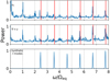 |
Fig. A.1. Power spectra of the GONG++ flow components and synthetic Rossby waves in the Stoneyhurst coordinate system at the equator. From the top to bottom panels are: the uy flows, radial vorticity, and uy component of synthetic Rossby waves (e.g., Hanson et al. 2020). Modes rotating at frequencies of multiples of Ωeq are indicated by the vertical gray lines. The vertical red lines show the rotational frequencies of the sectoral Rossby waves. We have considered only the m > 2 sectoral Rossby waves seen in the Sun. |
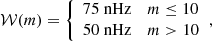
where T is the total observation time of the respective data set. A cosine bell filter was then applied to each m, centered on the theoretical dispersion ωr = −2Ωeq/(m + 1) with a tapering length of 35 nHz. The width 𝒲(m) of the filter follows,
 (A.2)
(A.2)
where the width narrows for m > 10 in order for the filter to not cross the zero frequency. We performed this filtering on ±3 aliases from the central ridge (which arise from the window function), as well as in the −m half-space.
With the solar equatorial Rossby modes removed, we reconstructed the flow maps by performing the inverse Fourier transform. The maps were then remapped onto the Stoneyhurst coordinate system. Figure A.2 shows the NS auto-correlation maps after the removal of the Rossby waves.
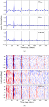 |
Fig. A.2. Top: temporal auto-correlation function of uy for HMI RDA, LCT, and GONG++ RDA. A signal can be seen to persist for at least four solar rotations. Statistical error bars are comparable to line thickness and hence are not shown. Bottom: 2D map of the uy auto-correlation maps, as a function of latitude and time lag. The deflection with latitude is consistent with differential rotation. The dashed vertical lines in each image indicate an integer equatorial rotation. |
While this filtering works near the equator, at higher latitudes the signal of the long-lived flows also becomes filtered. This is because the Rossby wave frequencies are independent of the differential rotation (latitude), while the advected flows are not. At higher m, the flow frequencies cross over into the Rossby mode filters at mid to high latitudes. This explains the lack of deflection in Fig. A.1. The vorticity of large-scale flows changes sign at the equator. The inflow vorticity is weaker than the divergence (factor 5, Hindman et al. 2009) and comparable to the Rossby waves. This means that, with or without filtering, obtaining a mean image of the inflow vorticity through our methodology (in the Northern or Southern Hemisphere) is difficult.
Appendix B: Mode fitting methodology
The estimates on the parameters Λm in Eq. (6) are determined by minimizing the negative of the log-likelihood function,
 (B.1)
(B.1)
where ωk is the kth frequency bin within the frequency window from (m − 1/2)Ωλ to (m + 1/2)Ωλ consisting of K frequencies.
The minimization of Jλ, m and the estimates on the error of the fits were computed from samples drawn by Markov chain Monte Carlo (MCMC) methods. The priors on the frequencies are ωm ∈ [mΩλ − Ωλ/2, mΩλ + Ωλ/2], where Ωλ is specified by the Snodgrass rotation rate (Snodgrass & Ulrich 1990). The priors on Am and Bm are such that the MCMC samples were drawn from the set [0, 5maxP(λ, ω)]. The prior on the line width are Γm ∈ [2(ωk + 1 − ωk),Ωλ/2]. We utilized the python library emcee (Foreman-Mackey et al. 2013) with 100 walkers and 1000 steps. The first 200 steps were taken as burn-in, and we computed the 16th, 50th, and 84th percentiles from the remaining 800 steps. We verified these results with the semi-analytical method in Toutain & Appourchaux (1994). The results obtained through MCMC are presented here since the error calculations are more numerically stable for fits at higher m and λ.
All Figures
|
Fig. 1. Monthly sunspot number (SSN) for cycles 23 and 24. The observation period of the present study and references herein are highlighted for reference. |
| In the text | |
|
Fig. 2. Top: temporal auto-correlation function of the EW flows at the equator for HMI RDA, LCT, and GONG++ RDA. A signal is seen to persist for at least five solar rotations. Statistical error bars are comparable to line thickness and hence are not shown. Bottom: 2D map of the EW auto-correlation maps as a function of latitude and time lag. The deflection with latitude is qualitatively consistent with differential rotation. The dashed vertical lines in each image indicate multiples of the equatorial rotation period. |
| In the text | |
|
Fig. 3. Plot of |
| In the text | |
|
Fig. 4. Difference between the rotational frequencies of the long-lived EW signals in HMI RDA and the synodic frequencies of Doppler features ( |
| In the text | |
|
Fig. 5. Top: lifetime of the modes seen in the HMI RDA EW power spectrum. Middle: signal-to-noise ratio (Am/Bm). Bottom: background power |
| In the text | |
|
Fig. 6. Top panels: average flows around convergent features during the solar maximum of cycle 23. Each of the first three rows is a different component of the flow, from top to bottom: EW flows, NS flows, and divergence maps. The fourth row is the average unsigned magnetic field. Each column is the mean map at an integer rotation before and after the initial identification (0 CR, middle column). Bottom-left panel: monthly sunspot number as a function of year (blue), with the center of the one-year observation window overplotted (vertical black line) and window size shown (shaded gray region). Bottom-right panel: spatial correlation coefficient between the CR = 0 flow maps and the flow maps at time lag CR (EW: blue; NS: orange; ∇h ⋅ u: green). |
| In the text | |
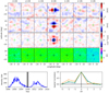 |
Fig. 7. Same as Fig. 6 except at the solar minimum between cycles 23 and 24. |
| In the text | |
|
Fig. 8. Spatial correlation coefficient between flow maps at CR = 0 and those at time lag CR, as a function of time and CR. The coefficients for the EW, NS, and divergence are shown in the top three panels, with the monthly sunspot number shown for reference in the bottom panel. The large-scale flows persist for a number of rotations during periods of high solar activity. |
| In the text | |
|
Fig. A.1. Power spectra of the GONG++ flow components and synthetic Rossby waves in the Stoneyhurst coordinate system at the equator. From the top to bottom panels are: the uy flows, radial vorticity, and uy component of synthetic Rossby waves (e.g., Hanson et al. 2020). Modes rotating at frequencies of multiples of Ωeq are indicated by the vertical gray lines. The vertical red lines show the rotational frequencies of the sectoral Rossby waves. We have considered only the m > 2 sectoral Rossby waves seen in the Sun. |
| In the text | |
|
Fig. A.2. Top: temporal auto-correlation function of uy for HMI RDA, LCT, and GONG++ RDA. A signal can be seen to persist for at least four solar rotations. Statistical error bars are comparable to line thickness and hence are not shown. Bottom: 2D map of the uy auto-correlation maps, as a function of latitude and time lag. The deflection with latitude is consistent with differential rotation. The dashed vertical lines in each image indicate an integer equatorial rotation. |
| In the text | |
Current usage metrics show cumulative count of Article Views (full-text article views including HTML views, PDF and ePub downloads, according to the available data) and Abstracts Views on Vision4Press platform.
Data correspond to usage on the plateform after 2015. The current usage metrics is available 48-96 hours after online publication and is updated daily on week days.
Initial download of the metrics may take a while.