| Issue |
A&A
Volume 643, November 2020
|
|
|---|---|---|
| Article Number | A101 | |
| Number of page(s) | 22 | |
| Section | Interstellar and circumstellar matter | |
| DOI | https://doi.org/10.1051/0004-6361/202038644 | |
| Published online | 10 November 2020 | |
Self-generated ultraviolet radiation in molecular shock waves
I. Effects of Lyman α, Lyman β, and two-photon continuum
1
Laboratoire de Physique de l’ENS, ENS, Université PSL, CNRS, Sorbonne Université, Université Paris-Diderot,
Paris,
France
e-mail: This email address is being protected from spambots. You need JavaScript enabled to view it.
2
LERMA, Observatoire de Paris, PSL Research Univ., CNRS, Sorbonne Univ.,
75014
Paris, France
3
Institut d’Astrophysique Spatiale, CNRS, Université Paris-Saclay,
Bât. 121,
91405
Orsay Cedex, France
Received:
12
June
2020
Accepted:
22
September
2020
Abstract
Context. Shocks are ubiquitous in the interstellar and intergalactic media, where their chemical and radiative signatures reveal the physical conditions in which they arise. Detailed astrochemical models of shocks at all velocities are necessary to understand the physics of many environments including protostellar outflows, supernova remnants, and galactic outflows.
Aims. We present an accurate treatment of the self-generated ultraviolet (UV) radiation in models of intermediate velocity (VS = 25–60 km s−1), stationary, weakly magnetised, J-type, molecular shocks. We show how these UV photons modify the structure and chemical properties of shocks and quantify how the initial mechanical energy is reprocessed into line emission.
Methods. We develop an iterative scheme to calculate the self-consistent UV radiation field produced by molecular shocks. The shock solutions computed with the Paris–Durham shock code are post-processed using a multi-level accelerated Λ-iteration radiative transfer algorithm to compute Lyman α, Lyman β, and two-photon continuum emission. The subsequent impacts of these photons on the ionisation and dissociation of key atomic and molecular species as well as on the heating by the photoelectric effect are calculated by taking the wavelength dependent interaction cross-sections and the fluid velocity profile into account. This leads to an accurate description of the propagation of photons and the thermochemical properties of the gas in both the postshock region and in the material ahead of the shock called the radiative precursor. With this new treatment, we analyse a grid of shock models with velocities in the range VS = 25–60 km s−1, propagating in dense (nH ≥ 104 cm−3) and shielded gas.
Results. Self-absorption traps Lyα photons in a small region in the shock, though a large fraction of this emission escapes by scattering into the line wings. We find a critical velocity VS ~ 30 km s−1 above which shocks generate Lyα emission with a photon flux exceeding the flux of the standard interstellar radiation field. The escaping photons generate a warm slab of gas (T ~ 100 K) ahead of the shock front as well as pre-ionising C and S. Intermediate velocity molecular shocks are traced by bright emission of many atomic fine structure (e.g. O and S) and metastable (e.g. O and C) lines, substantive molecular emission (e.g. H2, OH, and CO), enhanced column densities of several species including CH+ and HCO+, as well as a severe destruction of H2O. As much as 13–21% of the initial kinetic energy of the shock escapes in Lyα and Lyβ photons if the dust opacity in the radiative precursor allows it.
Conclusions. A rich molecular emission is produced by interstellar shocks regardless of the input mechanical energy. Atomic and molecular lines reprocess the quasi totality of the kinetic energy, allowing for the connection of observable emission to the driving source for that emission.
Key words: shock waves / radiative transfer / ISM: kinematics and dynamics / ISM: molecules / ISM: atoms / methods: numerical
© A. Lehmann et al. 2020
 Open Access article, published by EDP Sciences, under the terms of the Creative Commons Attribution License (https://creativecommons.org/licenses/by/4.0), which permits unrestricted use, distribution, and reproduction in any medium, provided the original work is properly cited.
1 Introduction
Shocks are the fingerprints of the dynamical state and evolution of the interstellar medium. From protostellar outflows and supernova explosions to galactic outflows, massive amounts of mechanical energy are injected at supersonic velocities into the entire range of galactic scales and interstellar phases (e.g. Raymond et al. 2020). Such flows inevitably form shocks which immediately alter the state of the gas via compression and viscous heating (Draine & McKee 1993), but they also give rise to a turbulent cascade and the generation of lower velocity shocks (e.g. Elmegreen & Scalo 2004). By reprocessing the initial kinetic energy into atomic and molecular lines, shocks produce invaluable tracers which carry information on the physical conditions of the shocked gas and on the source itself, including its energy budget, lifetime, and mass ejection rate (e.g. Reach et al. 2005; McDonald et al. 2012; Nisini et al. 2015). The comparison of detailed models with observations, therefore, allows one to address complex and unsolved issues such as the role of stellar and active galactic nuclei (AGN) feedback on the cycle of matter (Ostriker & Shetty 2011) and galaxy evolution (Schaye et al. 2015; Hopkins et al. 2018; Richings & Faucher-Giguère 2018) as well as the transfer of mass, momentum, and energy from the large scales to the viscous scale in turbulent multiphase media.
New examples of the ubiquity and modus operandi of interstellar shocks have emerged from recent observationsof extragalactic environments. In the Stefan’s Quintet collision, for instance, a large scale ~1000 km s−1 shock produces X-ray emission from the T > 106 K shock-heated gas. Warm molecular hydrogen, which should be destroyed at these temperatures, dominates the cooling in this region (Guillard et al. 2009), revealing the multiphase nature of the environment along with the necessary transfer of kinetic energy to lower velocity shocks. Interestingly, CO and [CII] lines have linewidths as large as 1000 km s−1, bearing the signature of the turbulent cascade driven in the post-shock gas by the large-scale shock (Appleton et al. 2017). Similarly, shocked, warm molecular hydrogen emission has also been observed in a sample of 22 radio galaxies in which star formation is quenched (Lanz et al. 2016). The authors suggest that shocks driven by the radio jets inject turbulence into the interstellar medium, which powers the luminous H2 line emission. Further opening occurred with the discovery of ubiquitous, powerful molecular outflows in local and high-redshift starburst galaxies (Veilleux et al. 2020; Hodge & da Cunha 2020). Molecular lines in galactic outflows are found with velocity dispersions in excess of 1000 km s−1, which can be seen as the signature of powerful turbulence generated by galactic winds (Falgarone et al. 2017). All of these examples reinforce the need for sophisticated and publicly accessible models capable of following the complex chemical and thermal evolution of shocks, down to the viscous scale, in a variety of physical conditions and for different input of mechanical energy.
Detailed shock models have long been developed for a variety of applications in the interstellar medium. Many works have been dedicated to modelling the heating, ionisation and radiative signatures of high velocity shocks (typically Vs >100 km s−1) propagating into the atomic environments (with ambient gas densities n < 1 cm−3) found in the intercloud medium (Pikel’Ner 1957), supernovae remnants (Cox 1972; Dopita 1976; Shull & McKee 1979) and Herbig–Haro objects (Raymond 1979). Particular attention has been given to accurately treating the radiative precursor, the region ahead of the shock affected by photons generated by the shock itself. Photoionisation in this region can alter the state of the gas before it enters the shock front and thus determines the shock initial conditions. Most recently, state of the art models draw from increasingly large atomic databases to accurately predict the spectra of radiative atomic shocks (Hartigan & Wright 2015; Sutherland & Dopita 2017; Dopita & Sutherland 2017).
There have also been extensive studies of shocks focusing on molecular environments. Early work by Field et al. (1968) and Aannestad (1973) considered molecular chemistry in low velocity shocks (Vs < 20 km s−1) in dense environments (n = 10–100 cm−3), with a focus on the survival of molecules through the shock-heated gas. These shocks are not hot enough to produce significant UV photons, and hence no treatment of a radiative precursor is required. In a series of works, Hollenbach & McKee (1979, 1980, 1989) treated the reformation of molecules in the cooling flow behind a fully dissociated shocked gas. By using the UV field calculated by a specialised atomic shock code, they were able to make an extensive study of shocks over both low and high velocities (Vs = 25–150 km s−1) and a broad range of densities (n = 10–109 cm−3). This work thoroughly detailed the key physical processes – such as photoionisation and dissociation, formation of H2 on dust, cooling from both atoms and molecules – which determine the structure and radiative characteristics of shocks in these environments. Further advancements were made by Neufeld & Dalgarno (1989) focusing on an accurate treatment of the UV radiative transfer, particularly Lyα and two-photon continuum, and its impact on molecular chemistry in intermediate velocity shocks (Vs = 60–100 km s−1) in dense media (n = 104–106 cm−3).
In the present paper, we revisit these pioneering and sophisticated developments by implementing the physics and chemistry of self-irradiated shocks in the Paris–Durham code1, a public and versatile state-of-the-art tool initially designed for the study of molecular shocks. Building on the recent updates of Lesaffre et al. (2013) and Godard et al. (2019) who focused on low velocity shocks (Vs ≤ 25 km s−1) irradiated by an external radiation field, we explore here an intermediate velocity range (25 km s−1 ≤ Vs ≤ 60 km s−1) where shocks are hot enough to generate significant UV radiation, yet cool enough to prevent the production of multi-ionised species. We present tracers for this velocity range, including atomic line emission, the Lyα and Lyβ counterparts, as well as tracers resulting from the complex molecular chemistry in the cooling flow. Infrared atomic and molecular lines are particularly timely given the wealth of data coming from the Atacama Large Millimeter/submillimeter Array (ALMA) and in anticipation of the James Webb Space Telescope (JWST).
The Paris–Durham shock code is introduced in Sect. 2 where we describe the updates implemented for this work. As a first step to compute the self-generated UV field we only treat the emission from atomic hydrogen. The corresponding three-level atomic model is outlined in Sect. 3. In Sect. 4, we describe the post-processed radiative transfer treatment to compute the shock generated radiation field. The effects of this radiation field on shocks at different velocities are shown in Sect. 5. We finally conclude by summarising our results in Sect. 6.
2 Shock model
In order to self-consistently compute a shock and the UV radiation field it generates, we iteratively solve these two components separately. We first generate a shock solution with the Paris–Durham shock code, which we describe in this section, then post-processthis output to compute the radiation field. We then run the shock code again in the presence of this radiation field and repeat until convergence.
2.1 J-type shocks
Interstellar shocks come in a variety of flavours, depending on the shock speed in relation to the signal speeds in the neutral and ionised components of the fluid (Draine & McKee 1993). We focus solely on single-fluid J-type (discontinuous) shocks in this work, because C-type (continuous) shocks do not reach the high temperatures required to generate significant UV radiation. In addition, for the conditions we consider (Table 2), in particular for weak magnetic fields, C-type shock velocities are bounded to velocities Vs < 25 km s−1 (see Fig. D1 in Godard et al. 2019). Figure 1 shows the typical evolution of the temperature and atomic and molecular hydrogen abundances in a J-type molecular shock. Viscous heating mediates an initial adiabatic jump in temperature up to a first plateau, whose temperature can be estimated using the Rankine-Hugoniot jump conditions, assuming an adiabatic index of 5∕3, shock velocity much larger than Alfven velocity (vA =  for magnetic field B and fluid mass density ρ) and fully molecular medium (mean molecular weight of 2.33 a.m.u.), as
 (1)
(1)
where Vs is the shock speed. At velocities greater than ~30 km s−1 interstellar shocks can reach temperatures sufficient to collisionally dissociate H2, with dissociation temperatureof 5.2 × 10⁴ K, and to collisionally excite atomic hydrogen, with electronic levels starting at ~ 1.2 × 10⁵ K. Atomic H is therefore produced in the hottest parts of the shock. Strong cooling due to Lyα excitations causes the temperature to drop from the peak to settle at T ≲ 104 K. This plateauis maintained until H2 reforms on grains deeper in the shock. In the transition between the adiabatic and second temperature plateau the excitation of H is strong enough to produce significant amounts Lyα photons. Flower & Pineau des Forêts (2010) estimated that a 30 km s−1 shock with preshock density nH = 2 × 105 cm−3 would produce a Lyα photon flux three orders of magnitude more than that of the standard UV interstellar radiation field (ISRF, Mathis et al. 1983). Such an effect calls for a detailed treatment of the UV radiative transfer in molecular shocks, and hence as a first step in this direction weconsider the addition of just one source of UV photons, the hydrogen atom. After summarising key aspects of the Paris–Durham shock code and outlining the updates used in this work we describe the 5-level model of hydrogen in Sect. 3.
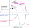 |
Fig. 1 Scheme of the profiles of temperature and UV production (top), and hydrogen abundances (bottom), for typical J-type molecular shocks. The shocked region (right of the dashed vertical line) is shown in log-scale of the distance in order to emphasise the initial adiabatic jump. |
2.2 Paris–Durham shock code
The Paris–Durham shock code gives the steady-state solution of the plane-parallel magnetohydrodynamics equations coupled with cooling functions and an extensive chemical reaction network appropriate to the molecular phases of the interstellar medium. The version usedin this work is that of Flower & Pineau des Forêts (2003), with updates described in Lesaffre et al. (2013), Godard et al. (2019) and here.
The code solves a set of coupled, first-order, ordinary differential equations – given by Flower (2010) – using the DVODE forward integration algorithm (Hindmarsh 1983) from some initial conditions. The dynamical variables, that is to say the density and velocity, are often parameters with initial values that we choose to explore, but the initial temperatureand chemical abundances are calculated by solving the chemical and thermal equations in a uniform slab for 107 years so that the material entering the shock is roughly in chemical and thermal equilibrium. We adopt the elemental abundances of Flower & Pineau des Forêts (2003) and put all of the species depleted on grain mantles into the gas phase (see Table 1). In order to integrate through the discontinuity in J-type shocks, the code employs an artificial viscosity treatment (Richtmyer & Morton 1957). This treatment has been verified to uphold the Rankine–Hugoniot relations, producing a smooth adiabatic jump in which momentum and energy are conserved.
In J-type shocks with molecular initial conditions the dominant source of atomic H in the hottest parts of the shock is the collisional dissociation of H2. The treatment of this process in the code has been detailed in Flower et al. (1996) and Le Bourlot et al. (2002), but we summarise it here in order to stress its importance for the accuracy of Lyα production in molecular shocks. The code takes into account the reduced energy required to dissociate H2 when excited in its rovibrational states. The dominant collision partners are H, H2, H+, He, and e−. Excitations to the dissociative triplet state b by collisionswith electrons has a rate coefficient given by
 (2)
(2)
where ET = 116 300 K is the excitation energy of the triplet state and  and
and  are the energy and fractional population of H2 in the rovibrational state v, J, respectively. For collisions with H, the dissociation rate coefficient is given by
 (3)
(3)
where ED = 52 000 K (4.48 eV) is the dissociation energy of H2. Rate coefficients for collisions with H2 are unknown for astrophysical conditions, but we use a rate eight times lower than for H collisions, as indicated by shock tube experiments (Jacobs et al. 1967; Breshears & Bird 1973).
The time-dependent populations of the rovibrational levels are solved in parallel with the dynamical and chemical variables as described inLe Bourlot et al. (2002) and Flower et al. (2003), allowing for collisional and radiative transitions between thelevels. In Appendix A, we check the effect of the number of levels treated has on the shock structure. We found that treating 150 levels is both computationally feasible and accurately models the H2 cooling and dissociation.
Fractional gas-phase elemental abundances used in this work.
2.3 Updates
As we post-process the UV radiative transfer (Sect. 4), the main update to the shock code is that it reads a given UV field at any point during the shock integration. Here we describe the modifications to account for this local field in addition to other updates on previous versions.
2.3.1 Photoreactions
Our treatment of photo-reactions (dissociation and ionisation) is slightly modified from Godard et al. (2019), because we don’t have to account for the attenuation of the radiation as this is done in the post-processed radiative transfer. Given the local radiation field energy density – calculated in the post-processed radiative transfer described in Sect. 4 – defined as
 (4)
(4)
where c is the speed of light and Jν is the angle averaged specific intensity at frequency ν, the photo-reaction rate is given by
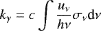 (5)
(5)
where h is Planck’s constant and σν is the frequency dependent cross-section. We use the cross-sections of Heays et al. (2017) rescaled onto a smaller wavelength grid by Tabone et al. (2020) for the most important photoreactions, the photo-ionisation of C, S, and Si, and both photo-ionisation and -dissociation of CH, OH, H2O, O2, and C2. For all other photoreactions, we use the form
 (6)
(6)
where α is the rate in the unattenuated standard ISRF, and Geff is the effective radiation parameter integrated over the whole frequency range (corresponding to wavelengths between 911–2400 Å), defined as
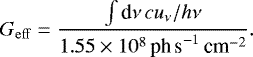 (7)
(7)
We note that Geff is simply the flux of photons normalised to the Mathis et al. (1983) ISRF.
2.3.2 Atomic H cooling
The energy lost due to the collisional excitation of the electronic levels of H is given by
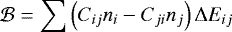 (8)
(8)
where the Cij and ΔEij are, respectively, the collision rates and energy differences between levels i and j, given in the next section, and the summation is taken over all pairs of levels. During the first shock iteration we compute the level populations ni by solving for statistical equilibrium treating only collisions and spontaneous emission. With no absorption or stimulated emission, this is an optically thin treatment. In subsequent iterations of the shock solution, we skip this computation and instead use the populations found during the post-processed radiative transfer described in Sect. 4. In this way the shock solution has a self-consistent treatment of cooling due to H.
2.4 Chemical network
Starting with the reaction network of Godard et al. (2019), we remove all adsorption and desorption reactions as we are interested in shocks fast enough to produce a UV field that removes all mantles via photodesorption. We then extend the network to include collisional ionisation and dissociation rates from Hollenbach & McKee (1989). These include ionisation of He, all metals and select molecules – OH, H2O, O2, CH, and CO – by collisions with H, H+, He, and electrons. We also include collisional dissociation by electrons for H2O, OH, and CO. These updates result in a chemical reaction network including 1256 reactions for 141 species.
3 Atomic hydrogen parameters
3.1 Collisional rates
In orderto study the UV field generated inside a molecular shock, we consider a three-level atomic hydrogen model including the Lyα (n = 2 → 1), Lyβ (n = 3 → 1), and Hα (n = 3 → 2) line transitions. The second level is divided into 2 sub-levels in order to model the two-photon emission from the 2s metastable state. The third level is also divided into two, grouped by orbitals with radiative transitions to either the 2p or 2s orbitals. This division of sub-levels is schematically shown in Fig. 2 and the values of the transition wavelengths, Einstein A coefficients, and energy differences ΔE for the six radiative transitions use atomic data from the NIST database (Kramida et al. 2019) and are listed in Table 2.
Collisions with electrons dominate most of the rates so we consider mostly H–e− collisions. The collisional de-excitation rates coefficients are given by
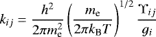 (9)
(9)
where ϒij is the effective collision strength. We fit ϒij data of Anderson et al. (2002) (given in Appendix B) as a temperature dependent power-law so that the de-excitation rate can be written as
 (10)
(10)
Collisional rate coefficients for the 2s to 2p orbitals are stronger for H–H+ collisions than H–e− collisions, so we also include these rates as given by Osterbrock & Ferland (2006) fit by the same power law Eq. (10). The collision rate parameters α, β, and energy differences ΔE for the 10 collisional transitions are listed in Table 2.
3.2 Non-local thermodynamic equilibrium parameter
A first characterisation of a radiative transfer problem is given by the non-local thermodynamic equilibrium (LTE) parameter
 (11)
(11)
for a line with collisional de-excitation rate Cij = kijnC where nC is the number density of the collisional partner. ɛ characterises the competition between the re-emission of an absorbed photon versus its destruction due to collisional de-excitation, and so approximates a photon destruction probability. If ɛ = 1, collisions dominate so that LTE holds and the radiation is thermal. As ɛ →0 the radiative transfer becomes increasingly difficult as the effects of scattering become important. In the fiducial shock we consider in Sect. 5.1 the Lyα emission is generated in gas with temperature T ~ 104 K and electron density ne ~ 103 cm−3, giving a non-LTE parameter ɛ ~ 10−14. This parameter appears in the solution of the statistical equilibrium equations and at such a low value can cause important rounding errors with double precision variables. We thus go to quad precision to avoid this problem. In the next section, we turn to the Accelerated Lambda Iteration method to overcome numerical difficulties caused by extreme optical depths.
Atomic hydrogen radiative and collisional transition parameters.
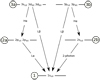 |
Fig. 2 Three level atomic hydrogen model and its radiative transitions. Statistical weights are g1 = 2, g2a = 6, g2b = 2, g3a = 12 and g3b= 6. |
4 Post-processed radiative transfer
In this section, we describe the post-processing of the Paris–Durham outputs to obtain the UV field at every point inside the shock as well as extending into the unshocked region ahead of the shock. This region ahead of the shock influenced by these UV photons is called the radiative precursor.
To briefly summarise, we first use the Accelerated Lambda Iteration (ALI) algorithm rendered necessary by the extreme optical depths in the Lyα transition. We then use the ALI calculated excited level populations to solve the radiative transfer for the two-photon continuum emission from the 2s metastable state. Finally the radiation field is extended into the radiative precursor. We give a summary of the ALI algorithm here, but for a detailed review see Hubeny (1992) and references therein.
4.1 Accelerated lambda iteration
We seek to calculate the angle-averaged UV intensity
 (12)
(12)
at each position, z, in the shockin order to compute the UV energy density (Eq. (4)) that is used to calculate photoelectric heating, photo-ionisation, and dissociation rates in the Paris–Durham shock code. For a plane-parallel semi-infinite slab, the specific intensity on a ray, Iμν, with angle μ = cosθ with respectto the slab normal satisfies the Radiative Transfer Equation (RTE)
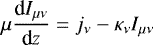 (13)
(13)
where the line emission coefficient for the transition i → j
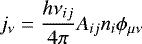 (14)
(14)
and line opacity
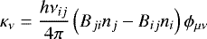 (15)
(15)
where ni and nj are the densities of the upper and lower levels of atomic hydrogen respectively, and Bij and Bji are the Einstein B coefficients. The Gaussian line profile is given by
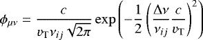 (16)
(16)
where the thermal velocity
 (17)
(17)
and frequency shift from the Doppler-shifted line centre, νij,
 (18)
(18)
where vz is the flow velocity in the shock propagation direction.
The level populations are needed to compute the emission coefficients, and are obtained by solving the Statistical Equilibrium (SE) equations
![Mathematical equation: \begin{align*}\dot{n}_i = 0 = & \sum_{j\neq i} \left(C_{ji} n_j - C_{ij} n_i\right) + \sum_{j > i} \left(A_{ji} n_j + \left(B_{ji}n_j - B_{ij}n_i \right)\bar{J}_{ij} \right) \nonumber \\ & - \sum_{j < i} \left(A_{ij} n_i + \left(B_{ij}n_i - B_{ji}n_j \right)\bar{J}_{ij} \right) \\[-21pt] \nonumber \end{align*}](/articles/aa/full_html/2020/11/aa38644-20/aa38644-20-eq23.png) (19)
(19)
where the  are the mean intensities, Jν, averaged over the line profile for that transition. In order to directly solve this at each position in the shock one would need to invert an enormous matrix with dimensions determined by the discretisation choices for the number of grid positions, frequencies, and angles. As this is computationally unrealistic, the usual strategy is to iterate between solving the RTE and SE equations. Our algorithm is summarised as follows:
- 1.
We initialise the populations by solving the SE equations with the
 set to zero. The populations are used to compute the source function
![Mathematical equation: \begin{eqnarray*} S_{ij} = \frac{j_{\nu}}{\kappa_{\nu}} = \frac{A_{ij}n_i}{B_{ji} n_j - B_{ij} n_i} \\[-14pt] \nonumber \end{eqnarray*}](/articles/aa/full_html/2020/11/aa38644-20/aa38644-20-eq26.png) (20)
(20)where we have assumed complete frequency redistribution, that is that the emission and absorption profiles are equal.
- 2.
The source function is used to solve the RTE along some ray, giving the specific intensity at each point in the shock for every desired frequency. The solution can be written in terms of an integral operator, Λμν, acting on the source function
![Mathematical equation: \begin{eqnarray*}I_{\mu\nu} = \Lambda_{\mu\nu} S_{ij}. \\[-14pt] \nonumber \end{eqnarray*}](/articles/aa/full_html/2020/11/aa38644-20/aa38644-20-eq27.png) (21)
(21)On a discrete grid this can be written
![Mathematical equation: \begin{eqnarray*}I_{\mu\nu}\left(z_l \right) = \sum_{l'} \Lambda_{\mu\nu}\left(z_l,z_{l'}\right) S_{ij}\left(z_{l'} \right) \\[-14pt] \nonumber \end{eqnarray*}](/articles/aa/full_html/2020/11/aa38644-20/aa38644-20-eq28.png) (22)
(22)emphasising that the intensity at any one point is coupled to the source function at all points, and that this coupling is encoded in Λμν.
- 3.
The intensity is used to compute the profile-integrated angle-averaged intensity for each transition
![Mathematical equation: \begin{eqnarray*}\bar{J}_{ij} = \frac{1}{2}\int_{-1}^1 \textrm{d}\mu \int I_{\mu\nu} \phi_{\mu\nu} \textrm{d}\nu. \\[-14pt] \nonumber \end{eqnarray*}](/articles/aa/full_html/2020/11/aa38644-20/aa38644-20-eq29.png) (23)
(23)We compute the intensity over two rays with angles θ = 0 and 180°, which has two advantages. Firstly it is coherent with the energetics of the plane-parallel shock in which the energy flux changes only along this direction. Secondly it avoids the non-convergence of the integral caused by emission adding up over infinite length rays near θ = 90°.
- 4.
The SE equations are solved to update the level populations. Without modification if we return to the first step and iterate to convergence we have the classical Lambda Iteration method, because the mean intensity in the SE equations is replaced by combining Eqs. (21) and (23)

where Λij – the profile-integrated angle-averaged Λμν – is the Λ-operator for this transition. This iteration scheme is known to be pseudo-convergent in systems with extreme optical depths. This effect is shown in Appendix C where we also verify the method against analytic solutions. The ALI algorithm overcomes such pseudo-convergence by splitting the Λij operator
 (26)
(26)where
 is the approximate Λ-operator. The iterative scheme is chosen such that at iteration n

Olson et al. (1986) demonstrated mathematically that a nearly optimal choice of
 is the diagonal of Λij. By inspecting Eq. (22), the diagonal encodes the local contribution of the source function to the intensity at a given point. The splitting in Eq. (27) can therefore be interpreted as solving the intensity exactly for the propagation within adjacent grid points while using the long range contribution from the previous iteration.
With this choice of
 the radiative terms in the SE equations become
 (29)
(29)Solving the SE equations with this modification, iteratively with Eq. (23) is the ALI algorithm.
- 5.
Before going back to step 1 we further increase the rate of convergence of the iterative scheme by way of the Ng acceleration algorithm (Ng 1974) as formulated by Olson et al. (1986). This algorithm extrapolates the excited populations based on the previous three iterations. We only take this step if the column densities of all levels vary monotonically over those previous iterations.
The approximate Λ-operator,  , as the diagonal of Λij emerges from the calculation of the intensities. In step 2, to solve the RTE along a given ray we use the method of short characteristics formulated by Paletou & Léger (2007) in which the intensity at position z is computed from the intensity at the upstream grid position, zu, and the source function as
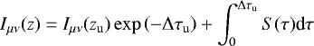 (30)
(30)
where the angle and frequency dependent upstream incremental optical depth is
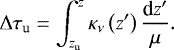 (31)
(31)
The integral in Eq. (30) is solved by assuming the source function is quadratic in the interval, interpolating on the grid points upstream (zu) and downstream (zd) of the point in question
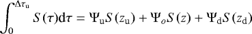 (32)
(32)
where the coefficients

where
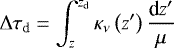 (36)
(36)
and

The diagonal of the Λ-operator is then given by Ψ0 integrated over all angles and frequencies weighted by the line profile. In Appendix D, we verify that the algorithm reproduces previous work on multi-level radiative transfer in idealised slabs.
4.2 Two-photon emission
The 2s metastable state of hydrogen cannot decay by a single photon process, and instead the 2s–1s transition proceeds by the emission of two photons. During the ALI computation this transition is treated as a resonance line with an Einstein coefficient A2ph = 8.2 s−1 in order to determine the population of the 2s orbital. This population is then used to compute the continuum emission by solving the RTE including only dust opacity and an emission coefficient
 (40)
(40)
where ψν is the functional form of the spectrum
 (41)
(41)
used in Shull & McKee (1979).
4.3 Radiative precursor and postshock extension
After computing the radiation field within the shock with the ALI method, we extend the radiation into the preshock by solving the RTE with the intensity at the shock front as a boundary condition. The ALI algorithm is not necessary in this region because of the low temperatures. In the first iteration, this escaping intensity impinges on a homogeneous slab entering the shock with flow velocity equal to the shock velocity. In subsequent iterations we use values of temperature and chemical composition computed with the Paris–Durham shock code.
To decide where to start the Paris–Durham integration the preshock is extended over a size, Lpre, such that the dust attenuates the field that escapes the shock, Geff,0, down to a negligible level compared to the ISRF. To do this we solve
 (42)
(42)
where κD is the dust opacity at the Lyα central wavelength.
We similarly extend the radiation further into the postshock by solving the RTE with the ALI output intensity as a boundary condition. This boundary is chosen at a location in the shock where the line radiative transfer has forced the Lyα energy into the wings but before dust attenuation takes effect.
In solving the RTE for the pre and postshock regions we include the opacity due to H, H2, and dust. While many H2 lines of the Lyman (B – X
– X ) and Werner (C1Πu – X
 ) band systems overlap with the Lyα or Lyβ emission, in practice we found only the v = 6 − 0 P(1) line to be of importance. In the first iteration, the H2 level populations are assumed thermal, and then we use the output of the shock code for self-consistent populations in subsequent iterations.
Fiducial shock parameters.
5 Results
To understand the impact of the new treatment of the self-generated UV field we first consider a single fiducial case of a typical shock. We highlight the impact of this treatment by comparing to a shock model run without self-generated UV. After considering the effects on one shock, we compute shocks at a range of velocities to analyse trends with velocity and give observable predictions for molecular shocks at intermediate velocities.
5.1 Fiducial case
As a fiducial case we consider a 40 km s−1 shock propagating into gas with total hydrogen density nH = 104 cm−3 and transverse magnetic field strength 10 μG. In order to emphasise the adiabatic plateau, we adopt here an artificial viscous length of 109 cm, 2 orders of magnitude smaller than the real viscous length deduced from the H2 –H2 collision cross-section. We note, however that the results are not dependent on this choice as long as the chosen viscous length is smaller than the real viscous length. In Table 3 we list the shock parameters. The shock acts to reprocess energy through heat into various atomic and molecular lines, dust emission, and to overcome energy barriers in chemical reactions. Some of this energy is also converted into magnetic energy. For the fiducial shock, all the components of this reprocessed energy are shown in Fig. 3. Excitation of molecules and atoms results in emission which escapes the shock and can be used to probe the shock properties. Excitation of H – though it is the largest component reprocessing almost half of the total energy flux – results in the emission of Lyα, Lyβ, and two-photon continuum UV radiation that is eventually absorbed by dust. Roughly half of this emission escapes ahead of the shock and is absorbed over a large distance set by the lengthscale of dust attenuation. The other half isreprocessed, in the cooling flow of the shock, into thermal energy via the photoelectric effect. Interestingly, the local cooling rate induced by collisional excitations of H and the subsequent interactions of Lyα, Lyβ, and two-photon continuum emission with the surrounding gas are not very different from the results obtained with an optically thin treatment of Lyα and Lyβ. The convoluted radiative transfer presented in the previous section is important only to determine the exact line profile and the spatial asymmetry of the H emission, that is the exact fractions of the radiative energy that travel ahead of the shock and in the postshock.
Profiles of temperature, density, and radiation field for this shock are shown in Fig. 4 with (solid) and without(thin dashed) the self-generated UV treatment included. The computation typically converges by 3 iterations ofshock and radiative transfer cycles. With no radiation field, the shock propagates into cold gas at ~10 K. After the adiabatic jump, seen in the middle panels of Fig. 4, dissociation of H2 mostly due to collisions with electrons produces atomic H with abundance ~1. Cooling due to H excitation by electron collisions – as discussed in Sect. 2.3.2 – then determines the transition down to a plateau at T ~ 104 K. The coolingis peaked in this transition as the temperature quickly drops too low for significant excitation of H, at which point O becomes the dominant coolant. This plateau is maintained until H2 reforms on dust grains and efficiently cools the gas along with other molecules – such as OH and CO – whose production follows the presence of H2.
With the self-generated UV treatment included, the photons that escape the shock front form a radiative precursor, heating the gas ahead of the shock to ~100 K over a distance of ~1017 cm (top left panel of Fig. 4), which is the length scale over which dust absorption fully attenuates the field. Photoionisation of C and S produces an increase in electron abundance entering the shock ~3 orders of magnitude more than the initial abundance. An increase in H+ also generates more electrons, resulting in stronger dissociation of H2 in the adiabatic plateau. Hence the cooling due to H excitation and the transition to the second temperature plateau occurs earlier than without the UV field. The position of this transition converges by the third iteration.
Strong self-absorption traps most of the Lyα photons near a peak of emission, seen in the lower centre panel of Fig. 4, between z = 1011–1014 cm where the UV flux is an order of magnitude more intense (Geff ~ 450) than that which escapes (Geff ~ 55). Emerging from the shock front, the Lyα, Lyβ, and two-photon fluxes are roughly 39, 1, and 14 times the ISRF. The flux escaping the trapped region is not symmetric. For Lyα, the rightward escaping photon flux is ~14% more than leftward. The rightward escaping photons are attenuated by dust in the postshock, generating an extended tail of warm molecular gas due to photoelectric heating. This tail remains above 10 K for a factor of ~3 longer than the first iteration.
Figures 5 and 6 show the radiation field in more detail. Figure 5 gives the flux around Lyα and Lyβ wavelengths at all positions in the precursor and postshock regions. It clearly shows strong absorption in the line cores forcing the energy to escape in the line wings. Figure 6 shows a few representative spectra at the shock front (z = 0), in the precursor (zpre = 1016 cm), at the peak of Lyα (z ~ 1012 cm) and Lyβ (z ~ 2 × 1011 cm) emission, and deep into the postshock (z = 1014 cm). The peaks of the wings in the precursor are shifted further away from line centre than the wings in the deep postshock after the peak of emission. This is because the H in the fluid before the peak is at higher temperatures than after the peak, and so it has a wider absorption profile. The precursor spectrum at Lyα shows deep absorption due to the cold H in this region at negative of the shock velocity. This is also seen in the Lyβ profile, as well as a deep absorption line due to H2 v = 6 − 0 P(1) Lyman band absorption, whose line centre Doppler-shifted by fluid velocity is shown in the Lyβ panels of Fig. 6 by the dashed grey vertical lines. The spectrum at the peak of Lyα emission shows the typical flat-top profile due to saturation effects of optically thick emission. The same saturation effects make the Lyβ spectrum start to show the flat-top profile. These peaks of emission emerge from the hot regions of the shock at T ~ 50 000 K.
Profiles of selected carbon-, oxygen-, sulphur-, and silicon-bearing species are shown in Fig. 7. The shock-generated UV strongly changes the preshock abundances and ionisation fraction of C, S, and Si. Without the UV field these three species all enter the shock mostly neutral, whereas they all become mostly ionised in the preshock. Oxygen chemistry is also strongly affected, with the photodissociation cross-sections of oxygen-bearing molecules O2, H2O, and OH overlapping Lyα, Lyβ, and/or the two-photon continuum. On the other hand, the photodissociation of CO proceeds via the indirect predissociation mechanism, requiring line absorption at specific wavelengths that do not overlap the H emission (van Dishoeck & Black 1988). Hence as the gas begins to be shocked most of the oxygen is contained in atomic O and CO. H2 is another molecule that survives the strong UV radiation, however in this case it is because there is not enough time spent in the radiative precursor for strong photodissociation to take place. When the fluid enters the hot shock front the temperatures and densities of the adiabatic jump and transition to the second plateau are not so different with or without the UV field, so the chemistry produces very similar abundances by z ~1012 cm. However, the UV persists with fluxes stronger than the typical ISRF, that is Geff > 1, until z ~1015 cm strongly affecting the chemistry in the region z ≳1013 cm. For example, the atomic ions C+, S+, and Si+ all remain more than 2 orders of magnitude higher than when UV photo-ionisation is not taken into account. Oxygen remains mostly atomic whereas without the UV treatment, there is a very strong formation of H2O in the this region. Finally, the peak of CH+ production at z ~1014 cm gives an abundance 3–4 orders of magnitude larger than without the UV treatment, before it settles at close to the same level after the UV has been attenuated. We address in the following sections how these differences in local abundances affect integrated quantities such as line emission and column densities.
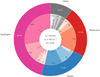 |
Fig. 3 Pathways of energy reprocessing in the fiducial shock (Table 3). This shows the energy lost due to excitation of atomic H, other atoms, molecules, and other processes as a percentage of the total energy flux. H2 chemistry involves cooling due to collisional dissociation and heating due to reformation. Other chemistry is mostly cooling due to collisional ionisation. |
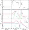 |
Fig. 4 Profiles of temperature (top), atomic, molecular, and ionised hydrogen densities (middle), and radiation field (bottom) for the fiducial shock (Table 3). For the radiation field, we show the total emission computed with Eq. (7) (violet) and the contributions to this total by Lyα (red), Lyβ (cyan), and two-photon continuum (blue). The left column shows quantities in the radiative precursor, with distance increasing towards the left (i.e. distance from the shock front), the middle column shows postshock quantities with distance increasing towards the right in log scale while the right column is the same as the middle but in linear scale. Thick lines show results including the UV treatment, while thin dashed lines have no UV included. |
5.2 Intermediate velocity shocks: Vs = 25–60 kms−1
5.2.1 Critical velocity
As a first step in determining the velocity at which the self-generated UV becomes important to treat we computed a small grid of shock models with velocities Vs = 25–60 km s−1 at every 5 km s−1, propagating into gas with total hydrogen density nH = 104 cm−3. All other parameters are the same as the fiducial shock, listed in Table 3. We leave the exploration of the dependence on density and other parameters to a forthcoming work.
The self-consistent converged temperature profiles are shown in Fig. 8. The peak temperature of the adiabatic jump rises with velocity according to Eq. (1). At Vs = 25 km s−1 the peak temperature is not strong enough to dissociate H2 to remove it asa significant coolant, and so the temperature drops to the postshock equilibrium without any plateaus. As the shock velocity increases, the dissociation occurs faster due higher temperatures. Thus atomic H is produced earlier with increasing velocity andso the transition to the second plateau occurs earlier due to the cooling by collisional excitations of H with electrons. Stronger H cooling leads to larger fluid densities in the second plateau. In turn, this leads to larger dust densities and a faster H2 formation rate, so thatH2 becomes thedominant coolant and the second plateau ends earlier with increasing velocity. The attenuation due to enhanced dust densities balances the stronger UV radiation fields here to give a nearly constant distance at which the shocks cool down to, say, 10 K.
The temperature profiles of the radiative precursors – left panel of Fig. 8 – show that heating due to the self-generated UV field starts to increase the preshock temperature above the initial value at a velocity between 30 and 35 km s−1. We ran a shock at 32 km s−1 to sample this transition with more detail. The UV strength parameter Geff emerging from the shock front (z = 0) is shown in Fig. 9. This shows a dramatic transition in the shock velocity range Vs = 30–32 km s−1 at which the emergent UV photon flux is stronger than the ISRF, that is Geff > 1. The adiabatic jump at this velocity heats the gas to high enough temperatures to simultaneously remove H2 as a strong coolant via collisional dissociation and excite H enough to produce strong Lyα fluxes. At Vs = 35 km s−1 the Lyα photon flux alone is ~10 times the ISRF. This presents the rather unique situation of having a slab of fully molecular material up against a boundary radiation field with Geff = 10–400 for shocks with velocities between 35 and 60 km s−1. This situation is generally not realised in photon-dominated regions with equivalent UV flux, because the broad spectrum of the ISRF is more effective at photodissociating H2 than the shock UV field concentrated around Lyα and Lyβ wavelengths. In such slabs, molecule formation thus takes place once the UV field has been strongly attenuated.
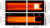 |
Fig. 5 Energy density of Lyα (top) and Lyβ (bottom) emission in the precursor (left) and postshock (right) regions. The vertical dashed lines give the positions of the cuts shown in Fig. 6: (PRE) in the precursor at zpre = 1016 cm, (PEAK) at the peaks of Lyα and Lyβ emission at z ~ 1012 cm and ~ 2 × 1011 cm respectively, and (DEEP) deeper in the postshock at z ~ 1014 cm. |
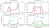 |
Fig. 6 Fluxes of Lyα (left) and Lyβ (right) in precursor (top) and postshock positions (bottom). The positions of the cuts – labelled PRE (red), PEAK (blue) and DEEP (green) – are shown in Fig. 5 by the vertical dashed lines, and the black lines give the fluxes at the shock front z = 0. Vertical greylines show line centres of Lyα and Lyβ (solid), H2 Lyman (dashed) and Werner (dotted) band absorption lines, with an emphasised v = 6 − 0 P(1) H2 line (thick dashed). The precursor vertical lines are Doppler-shifted by the shock velocity, whereas in the postshock panels they are shifted by flow velocity at the peak of the emission, Vz ~ 4 km s−1 for Lyα and Vz ~ 7 km s−1 for Lyβ. The arrows between the top and bottom panels highlights the velocity shift between the preshock gas and at peak emission. We note that none of the y-axes scales are the same. |
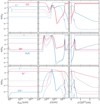 |
Fig. 7 Abundance profiles for selected species for the fiducial shock (Table 3) including (solid) and without (dashed) the self-generated UV. The left column shows quantities in the radiative precursor, with distance increasing towards the left (i.e. distance from the shock front), the middle column shows postshock quantities with distance increasing towards the right in log scale while the right column is the same as the middle but in linear scale. |
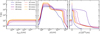 |
Fig. 8 Temperature profiles for the self-consistent shock solutions with shock velocities Vs = 25–60 km s−1 propagating into gas at nH = 104 cm−3. The left shows profiles in the radiative precursor, with distance increasing towards the left (i.e. distance from the shock front), the middle shows postshock profiles with distance increasing towards the right in log scale while the right is the same as the middle but in linear scale. Peak temperatures increase with increasing shock velocity (see Eq. (1)). |
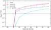 |
Fig. 9 Total UV flux as computed with Eq. (7) (violet) and the contributions to this total by Lyα (red), Lyβ (cyan), and two-photon continuum (blue) at the shock front (z = 0) for shocks with velocities VS = 25–60 km s−1 and preshock densities nH = 104 cm−3. The dashed horizontal line represents the standard interstellar radiation field. |
5.2.2 Shock length- and time-scales
In Figs. 10 and 11, we show the shock sizes and timescales at which the shock has cooled downto 200 K or 10 K. For the size scale, we also plot the size of radiative precursor that has been heated above 10 K. The sizes of both radiative precursor and postshock region are somewhat constant for shock velocities Vs ≥ 35, varying by less than a factor of 2 depending on the size criteria. This is because these sizes are essentially determined by the dust attenuation of the UV field.
5.2.3 Line emission
The shock observables that we consider here, that is selected atomic emission lines, rovibrational lines of H2, and column densities of various species, are all quantities obtained by integrating local quantities through the shock. The choice of where to end that integration therefore determines these quantities and the interpration of observations. For this work, we integrate until the gas falls down to 10 K, so that we integrate through shock-heated gas. There is also material ahead of the shock heated above 10 K in the radiative precursor. However, the precursor slabs computed here assume a uniform medium over large distances, which is not necessarily relevant in real astrophysical systems. Because it is unknown how realistic it is to include emission generated in the precursor, so we simply consider two cases: including this material or not.
In Fig. 12, we show the intensity of selected infrared fine structure lines generated in the shock heated gas. Most of these lines show a dramatic increase in intensity over the velocity range 30–60 km s−1 compared to lower velocity shocks. For example, the C+ (158 μm) and Si+ (34.8 μm) lines shows increases of more than 2 orders of magnitude once the UV becomes important. The C+ line also shows an increasing trend with velocity in this range, and has a strong contribution from the gas heated in the radiative precursor. The other fine structure lines show a remarkably constant intensity in this range. This figure then shows the general result that intermediate velocity molecular shocks produce strong emission in the fine-structure lines O(63.2 μm), O(145.3 μm), S(25.2 μm), and Si+ (34.8 μm).
Intensities of selected metastable atomic lines are shown in Fig. 13. More optical lines are accounted for in the model, but we show just the strongest lines for each species. As with the fine structure lines there are dramatic increases in these intensities over lower velocity shocks. In addition, there are stronger trends with velocity, for example the N+ (6583 Å) line varies by more than 3 orders of magnitude over the velocity range. A general result is that the intermediate velocity molecular shocks produce strong emission in the metastable lines O(6300 Å), C(9850 Å), and S+ (6731 Å).
In Fig. 14, we plot the intensities of the pure rotational lines S(0) up to S(4) of H2 as well as the v = 1 − 0 S(1) generated inthe shock-heated gas. Unlike the atomic lines, these lines do not show a significant increase compared their intensity from the 25 km s−1 shock. Theyare also remarkably constant over the velocity range, except for the contribution to the S(0) by the radiative precursor. Hence combined observations of atomic lines and H2 lines would be necessary to probe the different shock velocities in systems with an ensemble of shocks, such as in the turbulent cascade in the wakes galactic outflows or supernova shocks. These H2 lines lie in the observational bands of JWST and so could be used to interpret planned observations of such astrophysical systems.
The UV emission from atomic H – Lyα, Lyβ or two-photon continuum – are also possible observables. In Table 4 we list their fluxes that escape into the radiative precursor as well as the shock kinetic flux  . For shocks with velocities Vs ≥ 40 km s−1, 13–21% of the kinetic energy entering the shock comes back ahead of the shock in Lyα, Lyβ or two-photon emission. This UV emission can be absorbed by dust in the material ahead of the shock, which is often an unknown quantity in astrophysical systems. Combined with the previously discussed shock tracers, Table 4 could then be used to give a prediction of the maximum contribution to the Lyα emission from intermediate velocity shocks.
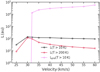 |
Fig. 10 Lengths at which the shocked regions cool down 10 K (black), or down to 200 K (red), and size of the radiative precursor computed as the gas layer ahead of the shock heated above 10 K (violet). |
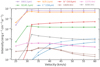 |
Fig. 12 Selected atomic fine-structure line intensities generated in the post-shock region (solid) or in the radiative precursor in addition to the post-shock (dashed). |
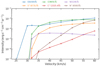 |
Fig. 13 Selected atomic meta-stable line intensities generated in the post-shock region (solid) or in the radiative precursor in addition to the post-shock (dashed). |
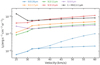 |
Fig. 14 Selected ro-vibrational H2 line intensities generated in the post-shock region (solid) or in the radiative precursor in addition to the post-shock (dashed). |
Energy flux (erg s−1 cm−2) emerging from the shock front in atomic H lines.
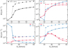 |
Fig. 15 Column densities of selected species. In each panel, we show the column density for postshock regions above 10 K (solid) and with the heated material in radiative precursor added to the postshock (dotted). |
5.2.4 Column densities
In addition to atomic and H2 line emission there are shock tracers in the molecular chemistry. Column densities of selected species are shown in Fig. 15. We show the column densities for postshock regions integrated until the gas cools to 10 K (solid lines) and also with the material in the radiative precursor added to shocked gas (dotted). Due to the extended warm tail produced by the UV there is an increase in the total H column density – by a factor ~3–4 in the postshock or an order of magnitude when including the preshock – for shocks with velocities Vs > 30 km s−1. Above this velocity, however, there is no significant correlation with velocity. This is due to the roughly constant shock-size, discussed in the previous section, over the velocity range once Lyα production becomes significant.
Some species show enhanced column densities when the UV field becomes strong at velocities Vs ≥ 32 km s−1. For example, column densities of CH+ and HCO+ are increased by more than 2 orders of magnitude by the end of the velocity range compared to their values at Vs = 30 km s−1. This is due to the larger abundances of C+ maintained by photoionisation deep in the postshock. The updated UV treatment may therefore allow us to consider shock models to interpret extragalactic ALMA observations of CH+ emission (Falgarone et al. 2017) as well as protostellar jet observations of HCO+ (e.g. Tafalla et al. 2010). In the other direction, photodissociation of H2O strongly reduces its column densities compared to molecular shocks at lower velocities. Observations involving oxygen chemistry have long stimulated the development of shock models. For instance, recent Herschel observations of protostellar environments reveal H2O abundances far too low to be explained with simple chemical models (e.g. Goicoechea et al. 2012; Kristensen et al. 2013; Karska et al. 2014, 2018). The precise origins of the emission of O2 (e.g. Yscıldscız et al. 2013; Chen et al. 2014; Melnick & Kaufman 2015) and O (Kristensen et al. 2017) have met with similar struggles. Mixtures of high velocity dissociative shocks, photodissociation regions, low velocity C-type shocks, and shocks irradiated by UV from either external sources or the shocks themselves have been invoked to explain these observations. The present work broadens the range of parameters of the Paris–Durham shock code to be used to study these problems, and shows how self-irradiated shocks could be a viable solution to explain low abundances of H2O and O2. The column densities of all these species (except CH+) in the heated precursor are larger than in the postshock because the precursors are orders of magnitude larger than the postshock, as seen in Fig. 10. H2O, OH, CO, and total H have more than a factor of 3 larger column in the radiative precursor than in the shocked gas. In summary, molecular shocks at intermediate velocities (Vs = 32–60 km s−1) have large column densities of CH+, HCO+, and CO while also having low column densities of H2O.
In Appendix F, we compare the column densities of selected species in Vs = 60 km s−1 shocks to the results of the shock models of Neufeld & Dalgarno (1989). The good agreement between the two works is a striking result given the decades of updates to chemical reaction networks and rates, computational methods, and the inclusion of the magnetic field in our work.
6 Conclusion
We have implemented a treatment of the UV radiative transfer including the atomic hydrogen lines Lyα, Lyβ, and the two-photon continuum in order to solve for self-irradiated molecular shocks at intermediate velocities using the Paris-Durham public shock code. The main results are summarised as follows:
-
A detailed treatment of radiative transfer is necessary to accurately compute the line profiles and escape of Lyα and Lyβ. However, to understand the energetic impacts of H excitation in these shocks it is sufficient to model the radiation with an optically thin treatment.
-
For preshock density nH = 104 cm−3, shocks with velocity Vs > 30 km s−1 produce a UV radiation field that escapes into the preshock gas with a Lyα photon flux stronger than the standard ISRF.
-
For shock velocities between 35 and 60 km s−1 the escaping UV photons give a radiation field parameter Geff ~ 10–400. In other words, the line and continuum emission of H alone carries as much as 400 times more photons than those contained in the entire ISRF. These photons escaping ahead of the shock heat the preshock gas in a radiative precursor over ~1017 cm to ~100 K.
-
The maximum contribution to Lyα emission for shocks with velocities 40–60 km s−1 is as large as 13–21% of the shock kinetic energy flux.
-
After HI emission, molecular emission is the second most important coolant in intermediate velocity shocks. In addition,these shocks have large column densities of CH+, HCO+, and CO while also having low column densities of H2O. These shocks may be useful in explaining low H2O abundances found in Herschel observations of protostellar environments.
-
Compared to lower velocity shocks, atomic fine structure and metastable emission lines are boosted by many orders of magnitude. For example, the O(63.2 μm) and S(25.2 μm) fine-structure lines and O(6300 Å) and C(9850 Å) metastable lines are particularly bright. Most fine structure lines are remarkably constant at intermediate shock velocities, but ratios of metastable lines could be used as a probe of shock velocity.
-
We predict intensities of ro-vibrational lines of H2. Many of these lines will be observable by JWST and hence this treatment will be critical for the interpretation of observations of phenomena with shocks at these velocities.
The present work shows that it is indeed important to properly model the UV radiation generated by the shock heated gas in order to extend models of molecular shocks to higher velocities. A forthcoming work will present the application of the present models for the interpretation of observations.
Acknowledgements
This research has received funding from the European Research Council through the Advanced Grant MIST (FP7/2017-2022, No. 742 719). We would also like to acknowledge the support from the Programme National “Physique et Chimie du Milieu Interstellaire” (PCMI) of CNRS/INSU with INC/INP co-funded by CEA and CNES.
Appendix A Number of H2 levels
To estimate the impact of the number of H2 levels on the shock structure we run 4 shock models with shock velocity Vs = 40 km s−1 and preshock density nH = 104 cm−3, varying the number of H2 levels treated: Nlev = 50, 100, 150 or 200. Otherwise, we use the same input parameters as the fiducial model (see Table 3). In Fig. A.1, we show the temperature and hydrogen abundance profiles for these shocks, which are reasonably converged when 150 levels are included. When treating 50 levels the dissociation of H2 is underpredicted by ~4 orders of magnitude, leading to the reformation of H2 to occur earlier and reduce the size of the shock by a factor of ~5.
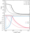 |
Fig. A.1 Profiles of temperature (top) and abundances of H and H2 (bottom) for Vs = 40 km s−1 shocks computed treating 50 (dot-dashed), 100 (dotted), 150 (dashed), or 200 (solid) levels of H2. |
Using 150 levels of H2, Fig. A.2 shows abundances profiles of H2 and H over the grid of shock models described in Sect. 5.2. At Vs = 25 km s−1, H2 is strongly dissociated in the adiabatic jump and H is the dominant species, but there is a transition at Vs = 30 km s−1 above which shocks dissociate H2 to a similar abundance x(H2) ~ 10−7.
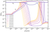 |
Fig. A.2 Profiles of H and H2 abundance for shocks with velocities Vs = 25–60 km s−1 and preshock density nH = 104 cm−3. |
Appendix B Atomic hydrogen parameters
Sub-level data of atomic hydrogen combined into three-level model taken from the NIST database (Kramida et al. 2019).
Radiative transition data for transitions between sub-levels of atomic hydrogen, taken from the NIST database (Kramida et al. 2019) except for two-photon Einstein coefficient (transition 9).
The three level model of hydrogen described in Sect. 3 is built by combining the data of the sub-levels with energies and statistical weights taken from the NIST database (Kramida et al. 2019) and listed in Table B.1. The statistical weights of the combined levels are the sum of the weights of their sub-levels
 (B.1)
(B.1)
The energies of the combined levels are the average energies of their sub-levels weighted by the statistical weights
 (B.2)
(B.2)
Similarly the Einstein coefficients of the combined levels, listed in Table 2, are the weighted average Einstein coefficients
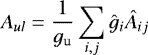 (B.3)
(B.3)
where the sum is over all the transitions from the sub-levels of the upper combined level to any of the sub-levels of the lower combined level. The sub-level transition data are taken from the NIST database (Kramida et al. 2019) – with the exception of the two-photon Einstein coefficient taken from Nussbaumer & Schmutz (1984) – and listed in Table B.2.
Atomic hydrogen sub-level effective collision strengths,  .
.
The effective collision strengths for de-excitation due to collisions with electrons are taken from Anderson et al. (2002), listed in Table B.3. The effective collision strengths, ϒA, have been modified in order to be applied to the fine structure of H. For all transitions n′ l′ j′→ nlj
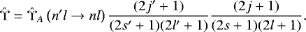 (B.4)
(B.4)
The de-excitation rate coefficient for the combined levels is the weighted average of the de-excitation rates coefficient for the sublevels

Hence the sum of the collision strengths for sublevel transitions gives the collision strength for the combined level transitions. We fit this combined collision strength with a power-law
 (B.8)
(B.8)
which allows us to express the rate coefficients as power-laws, Eq. (10), with the fit coefficients listed in Table 2.
Appendix C Two-stream approximation test
Our ALI transfer code is tested with the two-stream approximation test where the RTE of a homogeneous slab is solved along two rays with  . In addition,we impose a boundary condition that deep in the slab (when τ →∞) the source function equals the Planck function. This setup has analytic solution
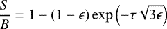 (C.1)
(C.1)
where B is the Planck function
 (C.2)
(C.2)
and ɛ is the non-LTE parameter
 (C.3)
(C.3)
For the homogeneous slab we use the Lyα radiative parameters listed in Table 2, and densities and temperatures typical for shock conditions: T =104 K, ne = 103 cm−3. This gives a non-LTE parameter ɛ ~ 10−14.
The result without using the ALI modification (that is, with Λ* = 0) is shown in Fig C.1. After 50 iterations the solution is still more than 6 orders of magnitude below the analytic solution. Using Λ* as defined by Eq. (34) we see in Fig. (C.2) that the solution converges onto the analytic solution before 50 iterations. Finally, using the Ng acceleration algorithm we get even faster convergence in Fig. C.3.
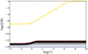 |
Fig. C.1 Two-stream approximation test: Lambda Iteration scheme. The yellow line is the analytic solution defined by Eq. (C.1). The blue line is the initial condition and the red line is the solution after 50 iterations. |
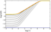 |
Fig. C.3 Same as Fig. C.1 but using the Accelerated Lambda Iteration scheme with Ng acceleration. We note that the red line is under the yellow line and cannot be seen. |
Appendix D Three-level hydrogen test
To further test the implementation of our ALI transfer code, we compare with the three-level benchmark problem of Avrett (1968). In this problem the radiative transfer is solved for a plane-parallel semi-infinite atmosphere with constant collisional de-excitation rates Cij = 105 s−1 for all three transitions and temperature 5000 K. The statistical weights are g1 = 2, g2 = 8, and g3 = 18. The transition frequencies are ν21 = 2.47 × 10¹⁵ Hz and ν31 = 2.93 × 10¹⁵ Hz. The Einstein coefficients are A21 = 4.68 × 10⁸ s−1, A31 = 5.54 × 10⁷ s−1, and A32 = 4.39 × 10⁷ s−1. The line profiles are Gaussian (Eq. (16)), we use an eight-ray Gaussian quadrature scheme and the boundary condition
 (D.1)
(D.1)
Finally we initialise the populations to be thermal.
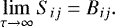
Figure D.1 shows the ratio of the source to Planck functions for the three transitions as a function of optical depth at the line centres of those transitions after 25 iterations. With Λ* defined by Eq. (34) and implementing Ng acceleration on the source functions the solutions have converged after this many iterations. The solutions show good agreement with the tabulated solutions of Avrett (1968).
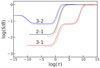 |
Fig. D.1 25th iteration of the three-level benchmark problem of Avrett (1968). Dotted lines are solutions tabulated in Avrett (1968). |
Appendix E Tables of results
Here we tabulate results for shock models in the velocity range Vs = 25–60 km s−1 described in Sect. 5.2. In Table E.1, we show the intensities escaping the shock front, which includes material in the shock down to 10 K as discussed in Sect. 5.2.3, of hydrogen and atomic fine structure and metastable lines. We also tabulate a subset of H2 rovibrational lines given as output by the code. Additional lines are available upon request. A selection of these lines are shown in Figs. 12–14. In Table E.2, we give column densities of a variety of species. Some of these column densities are shown in Fig. 15.
Line and two-photon continuum intensities (erg s−1 cm−2 sr−1) escaping the shock front as a function of shock velocity (km s−1) for shocks with preshock density nH = 104 cm−3.
Column densities (cm−2) of select species warmed above 10 K as a function of shock velocity (km s−1) for shocks with preshock density nH = 104 cm−3.
Appendix F Comparison with Neufeld & Dalgarno (1989)
In Table F.1 we give the column densities of several species obtained with the Paris–Durham shock code for 60 km s−1 shocks at three densities, nH = 104, 105, and 106 cm−3 in order to compare with the shock models of Neufeld & Dalgarno (1989). Our column densities are in rough agreement. The differences are due to H2 abundance, where Neufeld & Dalgarno find that cooling has reduced the temperature below 200 K before H2 can reform to more than a few percent. In our shock the gas is fully molecular in the reformation plateau above 200 K. This means the largest differences are in species influenced by the presence of H2. However, after three decades of development the two works are different. There are different computational methods, expanded chemical reaction networks and the inclusion of the magnetic field in our models. Hence it is striking how similar some of the column densities are with only a few species – for instance HCN, SO2, and SiO – varying by ~3 orders of magnitude or more in some models.
Column densities (cm−2) of warm gas, T > 200 K, predicted with the Paris–Durham shock code for shocks with velocity Vs = 60 km s−1 and ambient densities nH = 104, 105, and 106 cm−3 (L20), and comparison with the column densities predicted by Neufeld & Dalgarno (1989) (ND89).
Appendix G Energetics decomposition
In Fig. G.1, we show the energy reprocessing pathways for shocks with velocities Vs= 30, 40, 50, and 60 km s−1 propagating into a medium with density nH = 104 cm−3. These figures clearly emphasise that the cooling due to excitation of atomic H becomes suddenly dominant between velocities Vs= 30 and 40 km s−1. They also show that non-H atomic and molecular cooling remain roughly equally important over the whole velocity range.
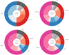 |
Fig. G.1 Pathways of energy reprocessing for shocks with velocities 30, 40, 50, and 60 km s−1 and preshock density nH = 104 cm−3. This shows the energy lost due to excitation of atomic H, other atoms, molecules, and other processes as a percentage of the total energy flux. H2 chemistry involves cooling due to collisional dissociation and heating due to reformation. Other chemistry is mostly cooling due to collisional ionisation. |
References
- Aannestad, P. A. 1973, ApJS, 25 [Google Scholar]
- Anderson, H., Ballance, C. P., Badnell, N. R., & Summers, H. P. 2002, J. Phys. B: At. Mol. Opt. Phys., 35, 1613 [NASA ADS] [CrossRef] [Google Scholar]
- Appleton, P. N., Guillard, P., Togi, A., et al. 2017, ApJ, 836, 76 [NASA ADS] [CrossRef] [Google Scholar]
- Avrett, E. H. 1968, in Resonance Lines in Astrophysics, eds. R. G. Athay, J. Mathis, & A. Skumanich (Boulder: National Center for Atmospheric Research), 27 [Google Scholar]
- Breshears, W. D., & Bird, P. F. 1973, Int. Symp. Combust., 14, 211 [CrossRef] [Google Scholar]
- Chen, J.-H., Goldsmith, P. F., Viti, S., et al. 2014, ApJ, 793, 111 [NASA ADS] [CrossRef] [Google Scholar]
- Cox, D. P. 1972, ApJ, 178, 143 [NASA ADS] [CrossRef] [Google Scholar]
- Dopita, M. A. 1976, ApJ, 209, 395 [NASA ADS] [CrossRef] [Google Scholar]
- Dopita, M. A., & Sutherland, R. S. 2017, ApJS, 229, 35 [NASA ADS] [CrossRef] [Google Scholar]
- Draine, B. T., & McKee, C. F. 1993, ARA&A, 31, 373 [NASA ADS] [CrossRef] [Google Scholar]
- Elmegreen, B. G., & Scalo, J. 2004, ARA&A, 42, 211 [NASA ADS] [CrossRef] [Google Scholar]
- Falgarone, E., Zwaan, M. A., Godard, B., et al. 2017, Nature, 548, 430 [NASA ADS] [CrossRef] [Google Scholar]
- Field, G. B., Rather, J. D. G., Aannestad, P. A., & Orszag, S. A. 1968, ApJ, 151, 953 [NASA ADS] [CrossRef] [Google Scholar]
- Flower, D. 2010, in Jets from Young Stars IV, eds. P. J. V. Garcia, & J. M. Ferriera, (Berlin-Heidelberg: Springer) Lect. Notes Phys., 793 161 [NASA ADS] [CrossRef] [Google Scholar]
- Flower, D. R., & Pineau des Forêts, G. 2003, MNRAS, 343, 390 [NASA ADS] [CrossRef] [Google Scholar]
- Flower, D. R., & Pineau des Forêts, G. 2010, MNRAS, 406, 1745 [Google Scholar]
- Flower, D. R., Pineau des Forêts, G., Field, D., & May, P. W. 1996, MNRAS, 280, 447 [NASA ADS] [CrossRef] [Google Scholar]
- Flower, D. R., Le Bourlot, J., Pineau des Forêts, G., & Cabrit, S. 2003, MNRAS, 341, 70 [NASA ADS] [CrossRef] [Google Scholar]
- Godard, B., Pineau des Forêts, G., Lesaffre, P., et al. 2019, A&A, 622, A100 [NASA ADS] [CrossRef] [EDP Sciences] [Google Scholar]
- Goicoechea, J. R., Cernicharo, J., Karska, A., et al. 2012, A&A, 548, A77 [NASA ADS] [CrossRef] [EDP Sciences] [Google Scholar]
- Guillard, P., Boulanger, F., Pineau des Forêts, G., & Appleton, P. N. 2009, A&A, 502, 515 [NASA ADS] [CrossRef] [EDP Sciences] [Google Scholar]
- Hartigan, P., & Wright, A. 2015, ApJ, 811, 12 [CrossRef] [Google Scholar]
- Heays, A. N., Bosman, A. D., & van Dishoeck, E. F. 2017, A&A, 602, A105 [NASA ADS] [CrossRef] [EDP Sciences] [Google Scholar]
- Hindmarsh, A. C. 1983, Scientific Computing (Amsterdam: North-Holland), 55 [Google Scholar]
- Hodge, J. A., & da Cunha, E. 2020, ArXiv e-prints, [arXiv:2004.00934] [Google Scholar]
- Hollenbach, D., & McKee, C. F. 1979, ApJS, 41, 555 [NASA ADS] [CrossRef] [Google Scholar]
- Hollenbach, D., & McKee, C. F. 1980, ApJ, 241, L47 [NASA ADS] [CrossRef] [Google Scholar]
- Hollenbach, D., & McKee, C. F. 1989, ApJ, 342, 306 [NASA ADS] [CrossRef] [Google Scholar]
- Hopkins, P. F., Wetzel, A., Kereš, D., et al. 2018, MNRAS, 480, 800 [NASA ADS] [CrossRef] [Google Scholar]
- Hubeny, I. 1992, in The Atmospheres of Early-Type Stars, (Springer, Berlin, Heidelberg), Lect. Notes Phys., 375 [CrossRef] [Google Scholar]
- Jacobs, T. A., Giedt, R. R., & Cohen, N. 1967, J. Chem. Phys., 47, 54 [NASA ADS] [CrossRef] [Google Scholar]
- Karska, A., Kristensen, L. E., van Dishoeck, E. F., et al. 2014, A&A, 572, A9 [NASA ADS] [CrossRef] [EDP Sciences] [Google Scholar]
- Karska, A., Kaufman, M. J., Kristensen, L. E., et al. 2018, ApJS, 235, 30 [NASA ADS] [CrossRef] [Google Scholar]
- Kramida, A., Yu. Ralchenko, Reader, J., & NIST ASD Team 2019, NIST Atomic Spectra Database (ver. 5.7.1), [Online]. Available: https://physics.nist.gov/asd [2020, May 26]. National Institute of Standards and Technology, Gaithersburg, MD. [Google Scholar]
- Kristensen, L. E., van Dishoeck, E. F., Benz, A. O., et al. 2013, A&A, 557, A23 [NASA ADS] [CrossRef] [EDP Sciences] [Google Scholar]
- Kristensen, L. E., Gusdorf, A., Mottram, J. C., et al. 2017, A&A, 601, A4 [NASA ADS] [CrossRef] [EDP Sciences] [Google Scholar]
- Lanz, L., Ogle, P. M., Alatalo, K., & Appleton, P. N. 2016, ApJ, 826, 29 [NASA ADS] [CrossRef] [Google Scholar]
- Le Bourlot, J., Pineau des Forêts, G., Flower, D. R., & Cabrit, S. 2002, MNRAS, 332, 985 [NASA ADS] [CrossRef] [Google Scholar]
- Lesaffre, P., Pineau des Forêts, G., Godard, B., et al. 2013, A&A, 550, A106 [NASA ADS] [CrossRef] [EDP Sciences] [Google Scholar]
- Mathis, J. S., Mezger, P. G., & Panagia, N. 1983, A&A, 128, 212 [NASA ADS] [Google Scholar]
- McDonald, M., Veilleux, S., & Rupke, D. S. N. 2012, ApJ, 746, 153 [NASA ADS] [CrossRef] [Google Scholar]
- Melnick, G. J., & Kaufman, M. J. 2015, ApJ, 806, 227 [NASA ADS] [CrossRef] [Google Scholar]
- Neufeld, D. A., & Dalgarno, A. 1989, ApJ, 340, 869 [Google Scholar]
- Ng, K.-C. 1974, J. Chem. Phys., 61, 2680 [Google Scholar]
- Nisini, B., Santangelo, G., Giannini, T., et al. 2015, ApJ, 801, 121 [NASA ADS] [CrossRef] [EDP Sciences] [Google Scholar]
- Nussbaumer, H., & Schmutz, W. 1984, A&A, 138, 495 [NASA ADS] [Google Scholar]
- Olson, G. L., Auer, L. H., & Buchler, J. R. 1986, JQRST, 35, 431 [Google Scholar]
- Osterbrock, D. E., & Ferland, G. J. 2006, Astrophys. Gaseous Nebulae Active Galactic Nuclei (Sausalito, CA: University Science Books) [Google Scholar]
- Ostriker, E. C., & Shetty, R. 2011, ApJ, 731, 41 [NASA ADS] [CrossRef] [Google Scholar]
- Paletou, F., & Léger, L. 2007, JQRST, 103, 57 [Google Scholar]
- Pikel’Ner, S. B. 1957, Sov. Astron., 1, 310 [Google Scholar]
- Raymond, J. C. 1979, ApJS, 39, 1 [NASA ADS] [CrossRef] [Google Scholar]
- Raymond, J. C., Chilingarian, I. V., Blair, W. P., et al. 2020, ApJ, 894, 108 [CrossRef] [Google Scholar]
- Reach, W. T., Rho, J., & Jarrett, T. H. 2005, ApJ, 618, 297 [NASA ADS] [CrossRef] [Google Scholar]
- Richings, A. J., & Faucher-Giguère, C.-A. 2018, MNRAS, 474, 3673 [Google Scholar]
- Richtmyer, R. D., & Morton, K. W. 1957, Difference Methods for Initial Value Problems (New York, NY: Interscience Publishers) [Google Scholar]
- Schaye, J., Crain, R. A., Bower, R. G., et al. 2015, MNRAS, 446, 521 [Google Scholar]
- Shull, J. M., & McKee, C. F. 1979, ApJ, 227, 131 [NASA ADS] [CrossRef] [Google Scholar]
- Sutherland, R. S., & Dopita, M. A. 2017, ApJS, 229, 34 [NASA ADS] [CrossRef] [Google Scholar]
- Tabone, B., Godard, B., Pineau des Forêts, G., Cabrit, S., & van Dishoeck, E. F. 2020, A&A, 636, A60 [CrossRef] [EDP Sciences] [Google Scholar]
- Tafalla, M., Santiago-García, J., Hacar, A., & Bachiller, R. 2010, A&A, 522, A91 [NASA ADS] [CrossRef] [EDP Sciences] [Google Scholar]
- van Dishoeck, E. F., & Black, J. H. 1988, ApJ, 334, 771 [NASA ADS] [CrossRef] [Google Scholar]
- Veilleux, S., Maiolino, R., Bolatto, A. D., & Aalto, S. 2020, ARA&A, 28, 2 [Google Scholar]
- Yscıldscız, U. A., Acharyya, K., Goldsmith, P. F., et al. 2013, A&A, 558, A58 [NASA ADS] [CrossRef] [EDP Sciences] [Google Scholar]
Available on the ISM platform https://ism.obspm.fr
All Tables
Sub-level data of atomic hydrogen combined into three-level model taken from the NIST database (Kramida et al. 2019).
Radiative transition data for transitions between sub-levels of atomic hydrogen, taken from the NIST database (Kramida et al. 2019) except for two-photon Einstein coefficient (transition 9).
Line and two-photon continuum intensities (erg s−1 cm−2 sr−1) escaping the shock front as a function of shock velocity (km s−1) for shocks with preshock density nH = 104 cm−3.
Column densities (cm−2) of select species warmed above 10 K as a function of shock velocity (km s−1) for shocks with preshock density nH = 104 cm−3.
Column densities (cm−2) of warm gas, T > 200 K, predicted with the Paris–Durham shock code for shocks with velocity Vs = 60 km s−1 and ambient densities nH = 104, 105, and 106 cm−3 (L20), and comparison with the column densities predicted by Neufeld & Dalgarno (1989) (ND89).
All Figures
|
Fig. 1 Scheme of the profiles of temperature and UV production (top), and hydrogen abundances (bottom), for typical J-type molecular shocks. The shocked region (right of the dashed vertical line) is shown in log-scale of the distance in order to emphasise the initial adiabatic jump. |
| In the text | |
|
Fig. 2 Three level atomic hydrogen model and its radiative transitions. Statistical weights are g1 = 2, g2a = 6, g2b = 2, g3a = 12 and g3b= 6. |
| In the text | |
|
Fig. 3 Pathways of energy reprocessing in the fiducial shock (Table 3). This shows the energy lost due to excitation of atomic H, other atoms, molecules, and other processes as a percentage of the total energy flux. H2 chemistry involves cooling due to collisional dissociation and heating due to reformation. Other chemistry is mostly cooling due to collisional ionisation. |
| In the text | |
|
Fig. 4 Profiles of temperature (top), atomic, molecular, and ionised hydrogen densities (middle), and radiation field (bottom) for the fiducial shock (Table 3). For the radiation field, we show the total emission computed with Eq. (7) (violet) and the contributions to this total by Lyα (red), Lyβ (cyan), and two-photon continuum (blue). The left column shows quantities in the radiative precursor, with distance increasing towards the left (i.e. distance from the shock front), the middle column shows postshock quantities with distance increasing towards the right in log scale while the right column is the same as the middle but in linear scale. Thick lines show results including the UV treatment, while thin dashed lines have no UV included. |
| In the text | |
|
Fig. 5 Energy density of Lyα (top) and Lyβ (bottom) emission in the precursor (left) and postshock (right) regions. The vertical dashed lines give the positions of the cuts shown in Fig. 6: (PRE) in the precursor at zpre = 1016 cm, (PEAK) at the peaks of Lyα and Lyβ emission at z ~ 1012 cm and ~ 2 × 1011 cm respectively, and (DEEP) deeper in the postshock at z ~ 1014 cm. |
| In the text | |
|
Fig. 6 Fluxes of Lyα (left) and Lyβ (right) in precursor (top) and postshock positions (bottom). The positions of the cuts – labelled PRE (red), PEAK (blue) and DEEP (green) – are shown in Fig. 5 by the vertical dashed lines, and the black lines give the fluxes at the shock front z = 0. Vertical greylines show line centres of Lyα and Lyβ (solid), H2 Lyman (dashed) and Werner (dotted) band absorption lines, with an emphasised v = 6 − 0 P(1) H2 line (thick dashed). The precursor vertical lines are Doppler-shifted by the shock velocity, whereas in the postshock panels they are shifted by flow velocity at the peak of the emission, Vz ~ 4 km s−1 for Lyα and Vz ~ 7 km s−1 for Lyβ. The arrows between the top and bottom panels highlights the velocity shift between the preshock gas and at peak emission. We note that none of the y-axes scales are the same. |
| In the text | |
|
Fig. 7 Abundance profiles for selected species for the fiducial shock (Table 3) including (solid) and without (dashed) the self-generated UV. The left column shows quantities in the radiative precursor, with distance increasing towards the left (i.e. distance from the shock front), the middle column shows postshock quantities with distance increasing towards the right in log scale while the right column is the same as the middle but in linear scale. |
| In the text | |
|
Fig. 8 Temperature profiles for the self-consistent shock solutions with shock velocities Vs = 25–60 km s−1 propagating into gas at nH = 104 cm−3. The left shows profiles in the radiative precursor, with distance increasing towards the left (i.e. distance from the shock front), the middle shows postshock profiles with distance increasing towards the right in log scale while the right is the same as the middle but in linear scale. Peak temperatures increase with increasing shock velocity (see Eq. (1)). |
| In the text | |
|
Fig. 9 Total UV flux as computed with Eq. (7) (violet) and the contributions to this total by Lyα (red), Lyβ (cyan), and two-photon continuum (blue) at the shock front (z = 0) for shocks with velocities VS = 25–60 km s−1 and preshock densities nH = 104 cm−3. The dashed horizontal line represents the standard interstellar radiation field. |
| In the text | |
|
Fig. 10 Lengths at which the shocked regions cool down 10 K (black), or down to 200 K (red), and size of the radiative precursor computed as the gas layer ahead of the shock heated above 10 K (violet). |
| In the text | |
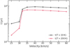 |
Fig. 11 Shock timescales for the same criteria as Fig. 10. |
| In the text | |
|
Fig. 12 Selected atomic fine-structure line intensities generated in the post-shock region (solid) or in the radiative precursor in addition to the post-shock (dashed). |
| In the text | |
|
Fig. 13 Selected atomic meta-stable line intensities generated in the post-shock region (solid) or in the radiative precursor in addition to the post-shock (dashed). |
| In the text | |
|
Fig. 14 Selected ro-vibrational H2 line intensities generated in the post-shock region (solid) or in the radiative precursor in addition to the post-shock (dashed). |
| In the text | |
|
Fig. 15 Column densities of selected species. In each panel, we show the column density for postshock regions above 10 K (solid) and with the heated material in radiative precursor added to the postshock (dotted). |
| In the text | |
|
Fig. A.1 Profiles of temperature (top) and abundances of H and H2 (bottom) for Vs = 40 km s−1 shocks computed treating 50 (dot-dashed), 100 (dotted), 150 (dashed), or 200 (solid) levels of H2. |
| In the text | |
|
Fig. A.2 Profiles of H and H2 abundance for shocks with velocities Vs = 25–60 km s−1 and preshock density nH = 104 cm−3. |
| In the text | |
|
Fig. C.1 Two-stream approximation test: Lambda Iteration scheme. The yellow line is the analytic solution defined by Eq. (C.1). The blue line is the initial condition and the red line is the solution after 50 iterations. |
| In the text | |
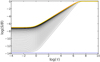 |
Fig. C.2 Same as Fig. C.1 but using the Accelerated Lambda Iteration scheme. |
| In the text | |
|
Fig. C.3 Same as Fig. C.1 but using the Accelerated Lambda Iteration scheme with Ng acceleration. We note that the red line is under the yellow line and cannot be seen. |
| In the text | |
|
Fig. D.1 25th iteration of the three-level benchmark problem of Avrett (1968). Dotted lines are solutions tabulated in Avrett (1968). |
| In the text | |
|
Fig. G.1 Pathways of energy reprocessing for shocks with velocities 30, 40, 50, and 60 km s−1 and preshock density nH = 104 cm−3. This shows the energy lost due to excitation of atomic H, other atoms, molecules, and other processes as a percentage of the total energy flux. H2 chemistry involves cooling due to collisional dissociation and heating due to reformation. Other chemistry is mostly cooling due to collisional ionisation. |
| In the text | |
Current usage metrics show cumulative count of Article Views (full-text article views including HTML views, PDF and ePub downloads, according to the available data) and Abstracts Views on Vision4Press platform.
Data correspond to usage on the plateform after 2015. The current usage metrics is available 48-96 hours after online publication and is updated daily on week days.
Initial download of the metrics may take a while.