| Issue |
A&A
Volume 643, November 2020
|
|
|---|---|---|
| Article Number | A25 | |
| Number of page(s) | 10 | |
| Section | Planets and planetary systems | |
| DOI | https://doi.org/10.1051/0004-6361/202038583 | |
| Published online | 28 October 2020 | |
Transmission spectroscopy and Rossiter-McLaughlin measurements of the young Neptune orbiting AU Mic
1
Instituto de Astrofísica de Canarias (IAC),
38200
La Laguna,
Tenerife,
Spain
e-mail: This email address is being protected from spambots. You need JavaScript enabled to view it.
2
Departamento de Astrofísica, Universidad de La Laguna (ULL),
38206
La Laguna,
Tenerife,
Spain
3
Department of Earth and Planetary Sciences, Tokyo Institute of Technology,
2-12-1 Ookayama,
Meguro-ku,
Tokyo
152-8551, Japan
4
Queen Mary University,
London,
UK
5
Department of Earth Sciences, University of Hawai’i at Mänoa,
Honolulu,
Hawaii
96822, USA
6
Institut de Ciències de l’Espai (ICE, CSIC),
Campus UAB, Can Magrans s/n,
08193
Bellaterra, Spain
7
Institut d’Estudis Espacials de Catalunya (IEEC),
08034
Barcelona,
Spain
8
Department of Physics and Astronomy, George Mason University, 4400 University Drive,
MSN3F3,
Fairfax,
VA
22030, USA
9
University of Southern Queensland,
West St,
Darling Heights
QLD 4350, Australia
Received:
5
June
2020
Accepted:
6
August
2020
Abstract
AU Mic b is a Neptune-sized planet on an 8.47-day orbit around the nearest pre-main sequence (~20 Myr) star to the Sun, the bright (V = 8.81) M dwarf AU Mic. The planet was preliminary detected in Doppler radial velocity time series and recently confirmed to be transiting with data from the TESS mission. AU Mic b is likely to be cooling and contracting and might be accompanied by a second, more massive planet, in an outer orbit. Here, we present the observations of the transit of AU Mic b using ESPRESSO on the Very Large Telescope. We obtained a high-resolution time series of spectra to measure the Rossiter-McLaughlin effect, to constrain the spin-orbit alignment of the star and planet, and to simultaneously attempt to retrieve the planet’s atmospheric transmission spectrum. These observations allowed us to study, for the first time, the early phases of the dynamical evolution of young systems. We applied different methodologies to derive the spin-orbit angle of AU Mic b, and all of them retrieve values consistent with the planet being aligned with the rotation plane of the star. We determined a conservative spin-orbit angle λ value of −2.96−10.30+10.44 degrees, indicative that the formation and migration of the planets of the AU Mic system occurred within the disc. Unfortunately, and despite the large signal-to-noise ratio of our measurements, the degree of stellar activity prevented us from detecting any features from the planetary atmosphere. In fact, our results suggest that transmission spectroscopy for recently formed planets around active young stars is going to remain very challenging, if at all possible, for the near future.
Key words: planets and satellites: atmospheres – techniques: radial velocities – planets and satellites: formation – planets and satellites: individual: Au Mic
© ESO 2020
1 Introduction
Planetary physical and orbital properties are predicted to evolve over time as a result of external and internal forcing. In fact, the observed distributions of exoplanet sizes and semi-major axes suggest that many planets migrate from their initial birth locations. Migration can occur by torques from primordial discs or scattering by a second planet and circularisation by tides (Lin et al. 1996; Kley & Nelson 2012). Planets with gas envelopes also cool and contract as they radiate their initial entropy of formation; close-in planets can also lose gas due to elevated irradiation by the active young host star. The detection and characterisation of planets in their early formation stages (<1 Gyr) are essential to test models of these phenomena (Baruteau et al. 2016).
The detection of planets around young stars, however, is exceptionally challenging. Direct imaging methods are only sensitive to very massive planets at large separations and provide planet radii, but not masses. Doppler radial velocity methods may be poised to overcome elevated stellar noise (jitter) among young stars (e.g. Prato et al. 2008) in order to detect and measure masses of close-in giant planets, but most of these will not transit and hence planet radii cannot be determined. Astrometry, on the other hand, solves the inclination ambiguity in the mass determination of the radial velocity technique and it is complementary to it; however, only one planet detection with this method has been confirmed so far (Sahlmann et al. 2013). This is set to change upon the release of the astrometric solutions for ESA’s space telescope, Gaia, in the near future. Photometry from the Kepler space telescope has revealed transiting planets in 10–800 Myr old clusters (e.g. Mann et al. 2016), but clusters are distant and most host stars are too faint to measure masses via radial velocity (RV) and/or obtain detailed follow-up observations. On the other hand, members of young moving groups (dispersed associations with similar space motions, abundances, and ages) include exceptionally young (20–300 Myr), nearby (<50 pc) stars, many of which are pre-main sequence M dwarfs. The closest star known of this kind is AU Microscopii, an M-type member of the ~20 Myr-old β Pictoris moving group that is only at a distance of 9.8 pc. AU Mic has an edge-on debris disc with evidence of ongoing planet formation (e.g. Boccaletti et al. 2018; Daley et al. 2019). Radial velocities of AU Mic obtained with both optical and infrared spectrographs (Plavchan et al. 2020) suggest the presence of one or more giant planets with orbital periods between 10 and 60 days.
The TESS mission (Ricker et al. 2014) observed AU Mic for 27 days during Sector 1 of its prime survey. Three transits were identified by visual inspection, and their high significance was verified against different models for stellar noise and false positives (Plavchan et al. 2020). Two transits with a similar depth (0.3%) and duration (3 h) were assigned to a candidate b planet with an orbital period of 8.46 days and a radius of R = 0.375 ± 0.018 RJ. Ground-based radial velocity measurements place the object’s mass to be <0.18 MJ, leading to a bulk density <4.4g cm−3 (Plavchan et al. 2020). AU Mic b is possibly still contracting and perhaps posses an extended atmosphere. A third transit in the TESS light curve is within 1-σ of the predicted time for a stronger radial velocity planet candidate, with a period of 30.7 days.
AU Mic now stands out as the closest system with transiting planets around a pre-main sequence star. This permits precise measurements of an orbit, mass, and radius, which will allow us to test how early planet migration and evolution occurred in the system’s history. Moreover, it has a debris disc which presumably marks the orientation of the former protoplanetary disc. The star’s rotation axis, its disc, and the orbits of planets b and c seem highly aligned with our line of sight, but they might not be aligned with each other. The formation and migration of the planets within the original protoplanetary disc of AU Mic should leave the planets on orbits with low inclinations with respect to the stellar rotation axis. On the other hand, incipient or past scattering could leave one or more planets on orbits that are highly inclined to both the stellar equator and the disc, although this is not always the end result of scattering processes. The Rossiter-McLaughlin (RM) effect and Doppler tomography are excellent techniques to infer the obliquity and inclination of fast-rotating stars, such as AU Mic. Here we present spectroscopic observations of one transit of the inner planet, AU Mic b, to constrain the projected angle of the planet’s orbit with respect to the star’s rotation axis and to perform an initial exploration of possible chemical species (atomic and molecular) in its atmosphere.
2 Observations and data reduction
One transit of AU Mic b was observed using the high precision RV spectrograph ESPRESSO at the Very Large Telescope (VLT) in its standard setup (400–780 nm, 1 UT – HR, standard calibration), during the night of August 7, 2019. Data were taken continuously from 3:24 UT to 9:23 UT, with an exposure time of 200 s. A total of 88 on-target spectra were taken, of which 37 spectra were taken out of transit, while another 49 spectra were taken in-transit over the ~3.5 h that the transit lasted. In principle, this high-cadence sampling is an advantage, given that the star is active and variable for the modelling and removal of line profile changes. During the observations, the airmass varied from 1.03 to 2.37, passing through a minimum of 1.007 (the last two data points were taken at airmass ≥ 2.3 where the ADC corrector might have problems). Weather conditions were clear. The averaged signal-to-noise ratio (S/N) of the spectra per pixel, measured at order 104 (near the Na I doublet), was 93.9.
The spectra were extracted and calibrated using the standard ESO-Data Reduction Software (DRS). According to the ESPRESSO exposure time calculator (ETC), the resulting individual RV measurements, considering photon noise and the instrumental floor, should have been better than 1 m s−1. However, the extracted RVs have a median internal precision of 3.7 m s−1, resulting from the broadening of the spectral feature of AU Mic due to rotation and stellar activity. We note that Plavchan et al. (2020) report AU Mic to be very active relative to main-sequence dwarfs and find RV peak-to-peak variations using HARPS spectrograph data in an excess of 400 m s−1, which is primarily due to the rotational modulation of stellar activity.
We also used a second approach to retrieve the RV values during the observations. We applied SERVAL (Zechmeister et al. 2018) to the 2D ESPRESSO spectra produced by the DRS pipeline. SERVAL produces high-precision differential Doppler observations by computing them relative to a high S/N template (co-added outside transit spectra). Using SERVAL, we achieve a median internal precision of 4.3 m s−1. SERVAL also produces several activity indicators such as the differential line width (DLW) and chromaticitity index (CRX), which are useful for our analysis and interpretation.
3 The Rossiter-McLaughlin effect
The transit of an exoplanet in front of its rotating host star generates a detectable RV signal, as the planet blocks the corresponding rotational signal of a portion of the stellar disc. This regional signal is removed from the integration of the velocity over the entire star, known as the RM effect (Holt 1893; Rossiter 1924; McLaughlin 1924). The RM observation is a powerful and efficienttechnique for estimating the spin-orbit angle of exoplanetary systems (see Triaud 2017 and references therein for a comprehensive review).
3.1 Transit time series and stellar activity
The rotation period of AU Mic (4.8 days) has long been compared to the transit duration. Except for the occurrence of a flare, which is easy to identify in chromospheric emission lines, the changes in the spectrum due to photospheric features should be smooth during the ~6 h that our observations lasted. Therefore, any change in RV due to rotational modulation can be removed by interpolating the out-of-transit line-profile measurements.
The ESPRESSO times series, however, shows strong evidence of flares and stellar activity during the observations. Figure 1 shows a cut of an out-of-transit spectrum of AU Mic. The selected spectral region contains the Na I doublet (5891.7 and 5897.6 Å) and the He I line at 5877.2 Å. It can be readily identified in Fig. 1 that AU Mic presents strong signatures of stellar activity. The total flux on the Na I doublet has two components; a chromospheric emission core is superimposed on the much broader and deeper photospheric absorption line (Walkowicz et al. 2008). In comparison, for the stellar chromospheric emission line of He I, only an emission feature is visible. On top of that, these emission features vary with time during the transit of AU Mic b, making it challenging to retrieve the orbital and atmospheric planet properties. In Fig. 2, we plotted the time evolution of several parameters that need to be taken into account for the analysis of AU Mic b’s transit. In particular, the S/N of each of the individual spectra and the transit light curve of the chromospheric He I line (see Sect. 5), which we use as a proxy for stellar flares, are useful indicators to weigh the value of each observation for the RM determination.
3.2 RM calculation
There are two main techniques to measure RVs during the transit of an exoplanet and to obtain the RM signal. One approach relies on the template matching of the observed spectra (Butler et al. 1996; Zechmeister et al. 2018), and the other one is based on a Gaussian fit to the cross-correlation function (CCF) of the observed spectra with a binary mask (Pepe et al. 2002). Each approach leads to a different shaped RM signal, as is theoreticallydemonstrated in Boué et al. (2013).
To model the RM observation obtained using the CCF- DRS pipeline, we used the publicly available code ARoME (Boué et al. 2013) which is optimised to model the RM signal extracted through the CCF-based approach. To model the RM observations obtained from template matching using the SERVAL pipeline, we used the model based on the approach by Ohta et al. (2005), which is optimised to retrieve the RM signal from template matching. This model is implemented in the PyAstronomy python package.
For both analyses, we considered a second order polynomial trend to interpolate the out-of-transit RV data between ingress and egress. This trend is present in both RM observations either from CCF-DRS or SERVAL, however, with a different shape and strength. This trend could have several contributors, either from the planet’s Keplerian orbit, any possible systematics in the data, and also the stellar activity induced RV (Oshagh et al. 2018). Thus, during our fitting procedure (either with PyAstronomy or ARoMe), we consider the spin-orbit angle λ, projected stellar rotational velocity (v sin(i)), mid-transit time (T0), limb darkening coefficients, and parameters of the second order polynomials as our free parameters. The rest of the parameters1 required in the models are fixed to their reported values in the literature (Porb = 8.46321 days, Rp∕R⋆ = 0.0514, a∕R⋆ = 19.1, and impact parameter (b) = 0.16; Plavchan et al. 2020). Based on the time series shown in Fig. 2, and again for both analyses, one data point with a very low S/N value just prior to the transit ingress was discarded, and several data points affected by a strong flare during the egress (starting at 0.29 days from the mid transit till the end of transit) were given a low weight during the fitting procedure.
The best fit parameters and associated uncertainties in our fitting procedure are derived using a Markov chain Monte Carlo (MCMC) analysis, using the affine invariant ensemble sampler emcee (Foreman-Mackey et al. 2013). The prior on v sin (i) and T0 are controlled by Gaussian priors centred on the reported value in the literature and width according to the reported uncertainties, and the prior on spin-orbit angle is also controlled by a uniform (uninformative) prior between −180 and +180 degrees. These priors are also listed in Table 1. We randomly initiated the initial values for our free parameters for 30 MCMC chains inside the prior distributions. For each chain, we used a burn-in phase of 500 steps, and then again sampled the chains for 5000 steps. Thus, the results concatenated to produce 150 000 steps. We determined the best fitted values by calculating the median values of the posterior distributions for each parameter, based on the fact that the posterior distributions were Gaussian.
The posterior distributions for both analyses are given in Figs. A.1 and A.2, and the best fitted model (bothPyAstronomy and ARoME) analyses and RM observations (both DRS-CCF and SERVAL) are shown in Fig. 3. The DRS-CCF and ARoME analysis suggest that the planet is aligned (spin-orbit angle = 0), however, it overestimates the v sin (i) value in comparison to that from a spectral line analysis, as reported in Plavchan et al. (2020). On the other hand, the SERVAL and PyAstronomy analysis suggests a slightly misaligned planet (spin-orbit angle = −9 degrees), but it is consistent with zero within the error bar, and also estimated the v sin (i) to be consistent with the reported value from spectral analysis. We report all of these value in Table 1.
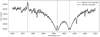 |
Fig. 1 Out-of-transit spectrum of AU Mic, zooming on the spectral region containing the Na I doublet at 5891.7 and 5897.6 Å, and the He I line at 5877.2 Å. The dashed lines indicate the central positions of these three lines. The red spectrum is the raw spectrum after DRS data subtraction, and the black spectrum results after the Molecfit telluric correction. |
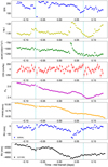 |
Fig. 2 From top to bottom: S/N of each of the individual spectra per pixel; the light curve of the chromospheric He I line at 5877.2 Å. The spectral line was integrated over a spectral range of 1.5 Å-wide; the dLW and CRX indices were derived using SERVAL; the light curve of the Hα line; the FWHM of CCF as estimated from DRS; the radial velocities were derived from SERVAL; and the radial velocities were derived from DRS. The vertical dashed cyan lines mark the predicted ingress and egress of transit of AU Mic b. |
Best fit derived values for the DRS+ARoME and SERVAL+PyAstronomy fits, with and without the use of Gaussian processes.
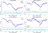 |
Fig. 3 Radial velocity time series derived from the DRS software (left columns) and SERVAL (right columns). Top panels: the best fit model to the RM is shown using the ARoME and PyAstronomy models, respectively. The red point is discarded in our analysis due to an anomalously low S/N, while the magenta points are given a lower weight in the RM fits due to being affected by a stellar flare. Lower panels: the data are the same but the fits incorporate the GP modelling. The different components of each best fit model are plotted in different colors and marked in the legend. |
3.3 Modelling RM with an additional Gaussian process
A Gaussian process is a general framework for modelling correlated noise (Rasmussen & Williams 2006), and it has shown its power and advantages in modelling and mitigating the stellar activity noise in RV observations (e.g. Haywood et al. 2014; Faria et al. 2016), in addition to photometric transit observations (e.g. Aigrain et al. 2016; Serrano et al. 2018), which assisted in detecting small-sized planetary signals embedded in the stellar activity noise.
Since our RM observations (either DRS or SERVAL) are clearly affected by the stellar activity noise (such as stellar spot occultations by the transiting planet and flares), we decided to incorporate GP to our RM modelling in order to perform a more robust fit and obtain more accurate estimates. We used the new implementation of GP in the celerite package (Foreman-Mackey et al. 2017) since some of the celerite kernels are well suited to describe different forms of stellar activity noises. To model the stellar noise in our data set, we selected the covariance as a Matern-3/2 Kernel. In order to train our GP, we first fitted this GP model to the differential line width (DLW) and He I light curve, which are the most affected observables by the flares occurring during our observation. This fitted GP allows us to have a better estimate on the prior time scale of the noise in our RV measurements. Here, we fitted our RM observations again; however, this time, we modelled the observed RMs (either from DRS or SERVAL) as the sum of the mean model and the noise. The mean model is the RM model (either AROME or PyASTRONOPMY, depending on which RM observations), and the noise was modelled as a Gaussian process with a Matern-3/2 covariance Kernel. The posterior samples for our model were obtained through MCMC using emcee (Foreman-Mackey et al. 2013). The prior on the RM models’ parameters were controlled as in the previous section; the prior on the GP time scale parameter was controlled by Gaussian priors centred on the fitted value from DLW and He I, and the prior on the GP amplitude was controlled by a uniform (uninformative) prior between 0.1 and 100 m s−1. These priors are also reported in Table 1. The posterior distributions for both analyses are given in Figs. A.3 and A.4, and the best fitted models’ (both PyAstronomy+GP and ARoME+GP) analyses and RM observations (both DRS-CCF and SERVAL) are shown in Fig. 3. We report all the best fitted values in Table 1.
The GP+RM model result in a much better fit as indicated by a significant decrease in the RMS of the residual (see reported RMS of residuals in Table 1). However, in order to perform a proper model comparison between RM only and the RM+GP model, we utilised MultiNest (Feroz et al. 2009) via the Dynesty package (Speagle 2020). Dynasty provides the Bayesian model log evidence (ln Z), and as suggested by Trotta (2008), we regard the difference between the two models to be strongly significant if their log evidence differs by ΔlnZ > 5. Our result shows that there are strong pieces of evidence supporting the idea of fitting the observed RM with a GP given their noise (Table 1).
The DRS-CCF and ARoME+GP as well as SERVAL and PyAstronomy+GP analyses both clearly demonstrate that the planet is prograde and aligned (within the uncertainties). However, both of them still overestimated the v sin (i) value; although, they are closer to the reported value from the spectral analysis than the one reported in Plavchan et al. (2020). The estimated v sin(i), considering their uncertainties, is compatible with the photometric rotation period of the star reported in Plavchan et al. (2020).
Brown et al. (2017) performed a comparison study and show that both models overestimate v sin(i) in comparison to the estimates obtained from spectral line broadening. They find that the overestimation can even reach as high as 5 km s−1 for fast-rotating stars. However, they find the estimated spin-orbit angles to be in strong agreement for both models. The overestimation of v sin(i) could be due to a variety of reasons. For instance, the RM signal can be affected by second-order effects such as the convective blueshift and granulation (Shporer & Brown 2011; Cegla et al. 2016), the stellar differential rotation (Hirano et al. 2011b; Hirano 2014; Albrecht et al. 2012; Cegla et al. 2016; Serrano et al. 2020), the microlensing effect caused by the transiting planet’s mass (Oshagh et al. 2013), the impact of a ringed exoplanet on the RM signal (Akinsanmi et al. 2018; de Mooij et al. 2017), the occulted stellar active regions (Oshagh et al. 2016, 2018), the non-occulted stellar active regions (Boldt et al. 2020), and also the inaccurate estimations of stellar limb darkening (Csizmadia et al. 2013; Yan et al. 2015). Some of these effects have a minor impact on the RM shape and amplitude, such as microlensing and a possible ring around the planet; however, others, such as the stellar active region occulation and stellar differential rotation, could cause a significant deformation of the RM shape and alter its amplitude. An underestimation of the planet radius, which was fixed in our analysis, in the bluer wavelength range of ESPRESSO (380−788 nm) in comparison to the TESS passband (600–1000 nm), could also lead to an overestimation of the v sin(i). None of these second-order effects are considered in ARoME or in PyAstronomy, and they could potentially be responsible for the overestimation of v sin(i). We note that the spectroscopic estimates are also model-dependent (choice of macroturbulence, etc.), and therefore they could also underestimate the v sin(i). An in depth investigation as to the reason for our overestimated v sin(i), however, is beyond the scope of this study. From all methodologies applied here, we chose a λ value of  degrees, based on Arome and GP, as a conservative determination of the spin-orbit angle, based on the data at hand.
4 Doppler tomography of AU Mic b
The Doppler tomography method (Collier Cameron et al. 2010; Watson et al. 2019) measures changes in the rotationally-broadened stellar line profiles due to partial occultation by the planet. Since cross-correlation functions (CCFs) of the observed spectra against a template reflect the mean profile of the stellar lines; one can probe the instantaneous velocity field on the stellar disc from the time-varying cross-correlations. The fit to this differential profile allows for a more precise and model-independent measurement of the free parameters: planet- and star-sized radius ratio, limb-darkening, projected obliquity angle, impact parameter, and duration (Strachan & Anglada-Escudé 2017).
For an independent measurement of the stellar obliquity, we analysed the time sequence of the CCFs returned by the DRS pipeline for the ESPRESSO spectra (see Fig. 4a for an observed CCF). To visualise the line-profile “variation”, we computed the residual cross-correlation map as a function of time; in doing so, we first normalised the CCF for each frame and combined the CCFs for frames taken outside the transit. We then subtracted the mean out-of-transit CCF from individual frames, yielding the residual CCF map in time.
Figure 4b displays the resultant residual CCF map. The two horizontal dashed lines represent the expected transit ingress and egress times. The residual map exhibits unexpectedly large modulations throughout our observations. This observed low-frequency modulation in the profile is not caused by AU Mic b’s transit, and the reasons for the large profile modulation are not known.
To remove this strong modulation, we applied a high-pass filtering in which we fitted the “out-of-transit” residual CCF by a quadratic function of time in each column of the residual CCF map. In interpolating the CCF variations during the transit, we subtracted the low-frequency modulation from the residual CCF map. Figure 4c shows the CCF map after the high-pass filtering. The CCF bump, representing the planet’s shadow of AU Mic b, is clearly seen in the map, moving from the blue edge tothe red edge of the original CCF (Fig. 4a). The trajectory of the shadow implies a prograde orbit of the transiting planet. The residual CCF map also suggests a flaring event happening around BJD = 2 458 702.81, which suddenly distorts the line profile for a relatively short interval. This is consistent with the large scatter in the observed RV data towards the end of the transit (Fig. 3).
To estimate the stellar obliquity λ, as well as other system parameters, from the residual CCF map, we performed an analysis of the RM effect. In brief, we fitted the positions of the planet shadow during the transit using a Gaussian and estimated the instantaneous Doppler position of the planet in the CCF profile for each frame (Fig. 5). Then, using the MCMC code to model the RM effect (Hirano et al. 2020), we fitted the positions of the planet’s shadow. The free adjustable parameters in the analysis are λ, v sin i, and the CCF centre γ, representing the peculiar RV of AU Mic. In many cases, γ is determined by precisely fitting the mean CCF profile outside the transit by the Gaussian. In the case of AU Mic, however, the mean out-of-transit CCF of the star is highly distorted and asymmetric (Fig. 4a), introducing an additional source of uncertainty in the CCF centre. A fit to the mean out-of-transit CCF led to γ = −4.16 ± 0.46 km s−1, but it is likely that the uncertainty is underestimated here due to the asymmetric CCF.
The MCMC fit to the observed planet shadow positions without any priors resulted in a degeneracy among λ, v sin i, and γ. Thus, we imposed a Gaussian prior on v sin i based on the spectroscopic value reported in the discovery paper (i.e. v sin i = 8.7 ± 2 km s−1). This analysis resulted in  degrees, which is consistent with the RV analysis results in Sect. 3.3. The best-fit model to the observed planet shadow positions is drawn by the solid red line in Fig. 5. To take the constraint on γ from the mean CCF profile into account, we also attempted an MCMC analysis, imposing priors on both v sin i and γ (= −4.16 ± 0.46 km s−1). This fit produced
  degrees, which is still compatible with the spin-orbit alignment of the system within 1.5 σ. Thus, we conclude that the RM fit and Doppler-tomography analyses yield fully consistent results, both independently supporting that the system has a low obliquity.
The large CCF modulation that is seen throughout the night of the transit is an unresolved issue. Figure 4d illustrates the residual CCF map after removing the planet shadow (panel c) from the original map. The CCF bump seen at ≈ − 5 km s−1 at the beginning of the observations moves on the stellar disc by ≈5 km s−1 at the end of the run. For comparison purposes, the AU Mic b planetary signal moves by ≈ 20 km s−1 during the shorter transit time. On the other hand, the rotation period of the star is estimated to be 4.863 days, and thus a star spot on the stellar surface should change its phase by 0.26∕4.863 = 0.053 during our observations. Assuming v sin i = 8−9 km s−1, this phase shift translates to the maximum Doppler shift of ≈ 2.9 km s−1 around the centre of the stellar disc. For reference purposes, we plotted this maximum shift of a CCF feature by stellar rotation in the same figure. The observed shift looks consistent with the rotation up to around the mid-transit time, but suddenly it changed the Doppler position by a few km s−1. At this point, we are not able to conclude that the observed modulation is an outcome of a giant spot on the stellar surface or a redistribution of visible active regions during the stellar rotation; further Doppler monitoring is needed to understand the peculiar behaviour of the CCF profile.
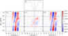 |
Fig. 4 Sample CCF profile during the night (panel a) and the residual (differential) CCF maps as a function of time (panels b–d). Panel b: illustrates the original residual CCF map after subtracting the mean out-of-transit CCF. The low-frequency modulations were subtracted based on the out-of-transit variations in panel c, in which the planet shadow is clearly seen. Panel d: residual map after the observed planet shadow is removed. The vertical dotted lines in panels a and c are the approximate CCF centre, representing the systemic RV of AU Mic. The near-vertical dashed linein panel d draws the maximum shift of the CCF bump by a spot-like feature on the stellar surface (≈ 3 km s−1 over 0.25 day). |
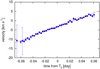 |
Fig. 5 Observed velocity positions of the planet’s shadow in the CCF profile (blue points) as a function of time. The solid red line indicates the best-fit RM model. |
5 Searching for atmospheric signatures
5.1 Transmission spectroscopy
A possible scenario for AU Mic b (still unconstrained, pending a precise mass determination) is the presence of an extended H/He atmosphere with a large transit cross-section, and although the nominal equilibrium temperature of the planet is 600–800 K, heating by XUV radiation from the host star (the Lx ∕Lbol of AU Mic is ~1000 × that of the Sun) could maintain a temperatureinversion and produce H-α absorption (Yan & Henning 2018). Here, we probe the composition and structure of the upper atmosphere of AU Mic b via transmission spectroscopy to try to constrain models of H/He escape, which are fundamental to explaining aspects of the mass-radius relation and radius distribution of exoplanets (Owen & Wu 2013; Fulton et al. 2017).
To search for planetary atmospheric features, we used the 1D spectral product of the DRS software, and follow the methodology employed in Casasayas-Barris et al. (2020). Prior to data analysis, the spectra are corrected for telluric absorptions using Molecfit (Smette et al. 2015; Kausch et al. 2015). After that, the analysis steps are as follows: (i) moving the spectra to the stellar rest frame, using the system parameters from Plavchan et al. (2020); (ii) constructing a master-out, high S/N, spectrum; (iii) dividing all spectra by the master-out and shifting them to the planet’s rest frame; (iv) combining all of the in-transit residual spectra (Casasayas-Barris et al. 2019, 2020); and (v) correcting for the sinusoidal interference pattern in the continuum that is sometimes seen in ESPRESSO (Casasayas et al., in prep.).
Unfortunately, stellar activity plays a big role in masking any possible planetary signal. Figure 6 shows the 2D residual maps of our data series near the Na I and He I lines. Strong structures in the data are seen both in and out of transit where one would expect a featureless map before and after the transit. The transmission spectrum for AU Mic b for this same spectral region is plotted in Fig. 7, where all three spectral lines are detected in emission, rather than in absorption if they were planetary signals in origin. The reason is the strong stellar flare that occurred during our observations near the transit egress, which lead to enhanced stellar chromospheric emission during transit. Thus, any possible planetary absorption is masked by this emission. We tried the approach of discarding data that are affected by flares, but nearly all of the spectra were affected at different levels and we were quickly left with no out-of-transit observations (this is also true for the analysis in Sect. 5.2).
To illustrate the effects of stellar activity, we have focused on the He I line at 5877.2 Å and we built a transit light curve centred around this line. To build the light curve, we again followed the methodology given in Casasayas-Barris et al. (2020), integrating the line over a 1.5 Å width interval. The light curve is shown in Fig. 2 and it traces up to three flares occuring during our observations. The light curve of other activity-affected lines, such as Hα, the Na I doublet, or the Ca H&K, correlates well with the He I (not shown), but being this is a weaker and narrower spectral features, it is easier to construct a high S/N light curve.
We have explored the full spectral range covered by ESPRESSO in search for detectable spectral absorption features, with no results. The spectral regions near the most prominent Na I, K I, Hα, Fe, or Mg absorption lines are always dominated by the effects of stellar activity. Thus, we have to conclude that transmission spectroscopy for AU Mic b, and for young forming planets around active young stars in general, is going to remain very challenging if not impossible for the near future.
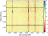 |
Fig. 6 Observed 2D maps of residual spectra around the Na I doublet in the stellar rest frame.The horizontal dashed lines mark the T1 and T4 transit contacts. The red-dashed lines mark the position of the Na I and He I lines. |
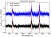 |
Fig. 7 AU Mic b transmission spectrum around the Na I doublet. The black dots show the original data with the respective error bars. The sinusoidal patter of the spectrum is due to the ESPRESSO wiggle pattern, which we did not correct here. |
5.2 Cross-correlation studies
Finally, we used the cross-correlation technique, following Stangret et al. (2020), to search for atmospheric signatures in AU Mic b. We started from the Molecfit telluric-corrected data, and we removed outliers in the spectrum by studying the time evolution of each pixel, then we normalised each order of the spectrum and masked the sky emission lines as well as strong telluric absorption lines. Finally, we applied SYSREM (Mazeh et al. 2007) to remove time- and wavelength-dependent trends in the spectral matrix. To calculate the high-resolution models used in the cross-correlation, we used petitRADTRANS (Mollière et al. 2019). For each studied individual atmospheric species, we cross-correlated a model with residuals using radial velocities in the range of +−200 km s−1 in steps of 0.5 km s−1, and we added all the orders. As with the transmission spectroscopy technique, we find that the stellar variability prevents us from exploring the planetary atmosphere. Our cross-correlation residual maps for Fe I as well as similar atomic and ionised species (see Fig. 8) are completely dominated by stellar chromospheric emission.
6 Conclusions
The proximity, brightness, youth, and the presence of a debris disc in AU Mic mean that it will quickly become a key system for studies of exoplanet formation and atmospheric evolution. Particularly interesting is the fact that at least one of its planets, AU Mic b, transits the star offering a unique opportunity to further constrain the physical properties of the system.
Following the recent discovery of AU Mic b, here we have conducted observations with ESPRESSO to measure the spin-orbit angle of the planet. We employed different data reduction and analysis techniques (Rossiter-McLaughlin effect measurement and Doppler tomography) to deal with the activity-affected data, which all give consistent results. AU Mic b seems to be well aligned with the rotation plane of its host star. This may not necessarily mean that the planetâs orbit is aligned with the current debris disc since there is a degeneracy in the angles on the sky. However, there are strong clues that this seems to be the case for AU Mic (Greaves et al. 2014; Watson et al. 2011). This means that the formation and migration of the planets of the AU Mic system occurred within the disc. AU Mic b is the third youngest (< 100 Myr) small planetwith a published measurement of its spin-orbit alignment, after DS Tuc b (Zhou et al. 2020) and HD 63433 b (Mann et al. 2020). Noticeably, all three planets show prograde and aligned orbits. Au Mic b’s properties are noticeably different from the other two Neptune planets with RM measuremets, which are HAT-P-11b (Hirano et al. 2011a) and GJ436b (Lanotte et al. 2014; Bourrier et al. 2018), both of which are misaligned and have eccentric orbits.
We have also explored the full spectral range covered by ESPRESSO in search for detectable spectral absorption features, with no results. The spectral region near the most prominent Na I, K I, Hα, He I, Fe, or Mg absorption lines is always dominated by the effects of stellar activity. Thus, we have to conclude that transmission spectroscopy for recently formed planets around active young stars is going to remain very challenging if not impossible for the near future, at least at optical wavelengths.
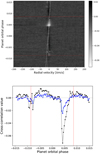 |
Fig. 8 Top: cross-correlation residuals map of FeI during the observations. The horizontal red-dashed lines show first (T1) and last (T4) transit contacts and the white-dashed lines show the expected planetary trail. Bottom: cross-correlation values at 0 km s−1 vs. time for Fe I (black), that is, a vertical cut on the top panel. Also shown is the cross-correlation evolution but for the Ca I (blue), showing a similar time evolution. |
Acknowledgements
The authors wish to thank an anonymous referee for his/her detailed comments to the original draft of this manuscript, which substantially improved the overall accuracy and clarity. This work is partly financed by the Spanish Ministry of Economics and Competitiveness through projects PGC2018-098153-B-C31 and ESP2016-80435-C2-2-R. This work was supported by JSPS KAKENHI Grant Number JP19K14783.
Appendix A Corner plots
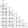 |
Fig. A.1 Posterior distributions for PyAstronomy. |
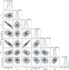 |
Fig. A.2 Posterior distributions for ARoME. |
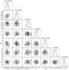 |
Fig. A.3 Posterior distributions for PyAstronomy+GP. |
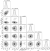 |
Fig. A.4 Posterior distributions ARoME+GP. |
References
- Aigrain, S., Parviainen, H., & Pope, B. J. S. 2016, MNRAS, 459, 2408 [NASA ADS] [Google Scholar]
- Akinsanmi, B., Oshagh, M., Santos, N. C., & Barros, S. C. C. 2018, A&A, 609, A21 [NASA ADS] [CrossRef] [EDP Sciences] [Google Scholar]
- Albrecht, S., Winn, J. N., Butler, R. P., et al. 2012, ApJ, 744, 189 [NASA ADS] [CrossRef] [Google Scholar]
- Baruteau, C., Bai, X., Mordasini, C., & Mollière, P. 2016, Space Sci. Rev., 205, 77 [NASA ADS] [CrossRef] [Google Scholar]
- Boccaletti, A., Sezestre, E., Lagrange, A. M., et al. 2018, A&A, 614, A52 [NASA ADS] [CrossRef] [EDP Sciences] [Google Scholar]
- Boldt, S., Oshagh, M., Dreizler, S., et al. 2020, A&A, 635, A123 [CrossRef] [EDP Sciences] [Google Scholar]
- Boué, G., Montalto, M., Boisse, I., Oshagh, M., & Santos, N. C. 2013, A&A, 550, A53 [NASA ADS] [CrossRef] [EDP Sciences] [Google Scholar]
- Bourrier, V., Lovis, C., Beust, H., et al. 2018, Nature, 553, 477 [NASA ADS] [CrossRef] [Google Scholar]
- Brown, D. J. A., Triaud, A. H. M. J., Doyle, A. P., et al. 2017, MNRAS, 464, 810 [NASA ADS] [CrossRef] [Google Scholar]
- Butler, R. P., Marcy, G. W., Williams, E., et al. 1996, PASP, 108, 500 [NASA ADS] [CrossRef] [Google Scholar]
- Casasayas-Barris, N., Pallé, E., Yan, F., et al. 2019, A&A, 628, A9 [NASA ADS] [CrossRef] [EDP Sciences] [Google Scholar]
- Casasayas-Barris, N., Pallé, E., Yan, F., et al. 2020, A&A, 635, A206 [NASA ADS] [CrossRef] [EDP Sciences] [Google Scholar]
- Cegla, H. M., Oshagh, M., Watson, C. A., et al. 2016, ApJ, 819, 67 [NASA ADS] [CrossRef] [Google Scholar]
- Collier Cameron, A., Bruce, V. A., Miller, G. R. M., Triaud, A. H. M. J., & Queloz, D. 2010, MNRAS, 403, 151 [NASA ADS] [CrossRef] [Google Scholar]
- Csizmadia, S., Pasternacki, T., Dreyer, C., et al. 2013, A&A, 549, A9 [NASA ADS] [CrossRef] [EDP Sciences] [Google Scholar]
- Daley, C., Hughes, A. M., Carter, E. S., et al. 2019, ApJ, 875, 87 [CrossRef] [Google Scholar]
- de Mooij, E. J. W., Watson, C. A., & Kenworthy, M. A. 2017, MNRAS, 472, 2713 [NASA ADS] [CrossRef] [Google Scholar]
- Faria, J. P., Haywood, R. D., Brewer, B. J., et al. 2016, A&A, 588, A31 [NASA ADS] [CrossRef] [EDP Sciences] [Google Scholar]
- Feroz, F., Hobson, M. P., & Bridges, M. 2009, MNRAS, 398, 1601 [NASA ADS] [CrossRef] [Google Scholar]
- Foreman-Mackey, D., Hogg, D. W., Lang, D., & Goodman, J. 2013, PASP, 125, 306 [CrossRef] [Google Scholar]
- Foreman-Mackey, D., Agol, E., Ambikasaran, S., & Angus, R. 2017, AJ, 154, 220 [NASA ADS] [CrossRef] [Google Scholar]
- Fulton, B. J., Petigura, E. A., Howard, A. W., et al. 2017, AJ, 154, 109 [NASA ADS] [CrossRef] [Google Scholar]
- Greaves, J. S., Kennedy, G. M., Thureau, N., et al. 2014, MNRAS, 438, L31 [NASA ADS] [CrossRef] [Google Scholar]
- Haywood, R. D., Collier Cameron, A., Queloz, D., et al. 2014, MNRAS, 443, 2517 [NASA ADS] [CrossRef] [Google Scholar]
- Hirano, T. 2014, Measurement of Spin-Orbit Angles for Transiting Systems: Toward an Understanding of the Migration History of Planets (Cham: Springer) [Google Scholar]
- Hirano, T., Narita, N., Shporer, A., et al. 2011a, PASJ, 63, 531 [NASA ADS] [Google Scholar]
- Hirano, T., Suto, Y., Winn, J. N., et al. 2011b, ApJ, 742, 69 [NASA ADS] [CrossRef] [Google Scholar]
- Hirano, T., Gaidos, E., Winn, J. N., et al. 2020, ApJ, 890, L27 [CrossRef] [Google Scholar]
- Holt, J. R. 1893, Astron. Astro-phys. (formerly The Sidereal Messenger), 12, 646 [Google Scholar]
- Kausch, W., Noll, S., Smette, A., et al. 2015, A&A, 576, A78 [NASA ADS] [CrossRef] [EDP Sciences] [Google Scholar]
- Kley, W., & Nelson, R. P. 2012, ARA&A, 50, 211 [Google Scholar]
- Lanotte, A. A., Gillon, M., Demory, B. O., et al. 2014, A&A, 572, A73 [NASA ADS] [CrossRef] [EDP Sciences] [Google Scholar]
- Lin, D. N. C., Bodenheimer, P., & Richardson, D. C. 1996, Nature, 380, 606 [NASA ADS] [CrossRef] [Google Scholar]
- Mann, A. W., Gaidos, E., Mace, G. N., et al. 2016, ApJ, 818, 46 [NASA ADS] [CrossRef] [Google Scholar]
- Mann, A. W., Johnson, M. C., Vanderburg, A., et al. 2020, AJ, 160, 179 [CrossRef] [Google Scholar]
- Mazeh, T., Tamuz, O., & Zucker, S. 2007, ASP Conf. Ser., 366, 119 [Google Scholar]
- McLaughlin, D. B. 1924, ApJ, 60, 22 [NASA ADS] [CrossRef] [Google Scholar]
- Mollière, P., Wardenier, J. P., van Boekel, R., et al. 2019, A&A, 627, A67 [NASA ADS] [CrossRef] [EDP Sciences] [Google Scholar]
- Ohta, Y., Taruya, A., & Suto, Y. 2005, ApJ, 622, 1118 [NASA ADS] [CrossRef] [Google Scholar]
- Oshagh, M., Boué, G., Figueira, P., Santos, N. C., & Haghighipour, N. 2013, A&A, 558, A65 [NASA ADS] [CrossRef] [EDP Sciences] [Google Scholar]
- Oshagh, M., Dreizler, S., Santos, N. C., Figueira, P., & Reiners, A. 2016, A&A, 593, A25 [NASA ADS] [CrossRef] [EDP Sciences] [Google Scholar]
- Oshagh, M., Triaud, A. H. M. J., Burdanov, A., et al. 2018, A&A, 619, A150 [NASA ADS] [CrossRef] [EDP Sciences] [Google Scholar]
- Owen, J. E., & Wu, Y. 2013, ApJ, 775, 105 [Google Scholar]
- Pepe, F., Mayor, M., Galland, F., et al. 2002, A&A, 388, 632 [NASA ADS] [CrossRef] [EDP Sciences] [Google Scholar]
- Plavchan, P., Barclay, T., Gagné, J., et al. 2020, Nature, 582, 497 [CrossRef] [Google Scholar]
- Prato, L., Huerta, M., Johns-Krull, C. M., et al. 2008, ApJ, 687, L103 [NASA ADS] [CrossRef] [Google Scholar]
- Rasmussen, C. E., & Williams, C. K. I. 2006, Gaussian Processes for Machine Learning (Cambridge: MIT press) [Google Scholar]
- Ricker, G. R., Winn, J. N., Vanderspek, R., et al. 2014, Proc. SPIE, 9143, 914320 [Google Scholar]
- Rossiter, R. A. 1924, ApJ, 60, 15 [Google Scholar]
- Sahlmann, J., Lazorenko, P. F., Ségransan, D., et al. 2013, A&A, 556, A133 [NASA ADS] [CrossRef] [EDP Sciences] [Google Scholar]
- Serrano, L. M., Barros, S. C. C., Oshagh, M., et al. 2018, A&A, 611, A8 [NASA ADS] [CrossRef] [EDP Sciences] [Google Scholar]
- Serrano, L. M., Oshagh, M., Cegla, H. M., et al. 2020, MNRAS, 493, 5928 [CrossRef] [Google Scholar]
- Shporer, A., & Brown, T. 2011, ApJ, 733, 30 [NASA ADS] [CrossRef] [Google Scholar]
- Smette, A., Sana, H., Noll, S., et al. 2015, A&A, 576, A77 [NASA ADS] [CrossRef] [EDP Sciences] [Google Scholar]
- Speagle, J. S. 2020, MNRAS, 493, 3132 [NASA ADS] [CrossRef] [Google Scholar]
- Stangret, M., Casasayas-Barris, N., Pallé, E., et al. 2020, A&A, 638, A26 [CrossRef] [EDP Sciences] [Google Scholar]
- Strachan, J. B. P., & Anglada-Escudé, G. 2017, MNRAS, 472, 3467 [NASA ADS] [CrossRef] [Google Scholar]
- Triaud, A. H. M. J. 2017, The Rossiter-McLaughlin Effect in Exoplanet Research (Springer Living Reference Work) (Berlin: Springer), 2 [Google Scholar]
- Trotta, R. 2008, Contemp. Phys., 49, 71 [Google Scholar]
- Walkowicz, L. M., Johns-Krull, C. M., & Hawley, S. L. 2008, ApJ, 677, 593 [NASA ADS] [CrossRef] [Google Scholar]
- Watson, C. A., Littlefair, S. P., Diamond, C., et al. 2011, MNRAS, 413, L71 [NASA ADS] [CrossRef] [Google Scholar]
- Watson, C. A., de Mooij, E. J. W., Steeghs, D., et al. 2019, MNRAS, 490, 1991 [CrossRef] [Google Scholar]
- Yan, F., & Henning, T. 2018, Nat. Astron., 2, 714 [NASA ADS] [CrossRef] [Google Scholar]
- Yan, F., Fosbury, R. A. E., Petr-Gotzens, M. G., Zhao, G., & Pallé, E. 2015, A&A, 574, A94 [NASA ADS] [CrossRef] [EDP Sciences] [Google Scholar]
- Zechmeister, M., Reiners, A., Amado, P. J., et al. 2018, A&A, 609, A12 [CrossRef] [Google Scholar]
- Zhou, G., Winn, J. N., Newton, E. R., et al. 2020, ApJ, 892, L21 [CrossRef] [Google Scholar]
ARoMe also requires the width of the CCF of the non-rotating star, which depends on the instrumental broadening, and we adjusted that according to the expected value from ESPRESSO based on its resolution.
All Tables
Best fit derived values for the DRS+ARoME and SERVAL+PyAstronomy fits, with and without the use of Gaussian processes.
All Figures
|
Fig. 1 Out-of-transit spectrum of AU Mic, zooming on the spectral region containing the Na I doublet at 5891.7 and 5897.6 Å, and the He I line at 5877.2 Å. The dashed lines indicate the central positions of these three lines. The red spectrum is the raw spectrum after DRS data subtraction, and the black spectrum results after the Molecfit telluric correction. |
| In the text | |
|
Fig. 2 From top to bottom: S/N of each of the individual spectra per pixel; the light curve of the chromospheric He I line at 5877.2 Å. The spectral line was integrated over a spectral range of 1.5 Å-wide; the dLW and CRX indices were derived using SERVAL; the light curve of the Hα line; the FWHM of CCF as estimated from DRS; the radial velocities were derived from SERVAL; and the radial velocities were derived from DRS. The vertical dashed cyan lines mark the predicted ingress and egress of transit of AU Mic b. |
| In the text | |
|
Fig. 3 Radial velocity time series derived from the DRS software (left columns) and SERVAL (right columns). Top panels: the best fit model to the RM is shown using the ARoME and PyAstronomy models, respectively. The red point is discarded in our analysis due to an anomalously low S/N, while the magenta points are given a lower weight in the RM fits due to being affected by a stellar flare. Lower panels: the data are the same but the fits incorporate the GP modelling. The different components of each best fit model are plotted in different colors and marked in the legend. |
| In the text | |
|
Fig. 4 Sample CCF profile during the night (panel a) and the residual (differential) CCF maps as a function of time (panels b–d). Panel b: illustrates the original residual CCF map after subtracting the mean out-of-transit CCF. The low-frequency modulations were subtracted based on the out-of-transit variations in panel c, in which the planet shadow is clearly seen. Panel d: residual map after the observed planet shadow is removed. The vertical dotted lines in panels a and c are the approximate CCF centre, representing the systemic RV of AU Mic. The near-vertical dashed linein panel d draws the maximum shift of the CCF bump by a spot-like feature on the stellar surface (≈ 3 km s−1 over 0.25 day). |
| In the text | |
|
Fig. 5 Observed velocity positions of the planet’s shadow in the CCF profile (blue points) as a function of time. The solid red line indicates the best-fit RM model. |
| In the text | |
|
Fig. 6 Observed 2D maps of residual spectra around the Na I doublet in the stellar rest frame.The horizontal dashed lines mark the T1 and T4 transit contacts. The red-dashed lines mark the position of the Na I and He I lines. |
| In the text | |
|
Fig. 7 AU Mic b transmission spectrum around the Na I doublet. The black dots show the original data with the respective error bars. The sinusoidal patter of the spectrum is due to the ESPRESSO wiggle pattern, which we did not correct here. |
| In the text | |
|
Fig. 8 Top: cross-correlation residuals map of FeI during the observations. The horizontal red-dashed lines show first (T1) and last (T4) transit contacts and the white-dashed lines show the expected planetary trail. Bottom: cross-correlation values at 0 km s−1 vs. time for Fe I (black), that is, a vertical cut on the top panel. Also shown is the cross-correlation evolution but for the Ca I (blue), showing a similar time evolution. |
| In the text | |
|
Fig. A.1 Posterior distributions for PyAstronomy. |
| In the text | |
|
Fig. A.2 Posterior distributions for ARoME. |
| In the text | |
|
Fig. A.3 Posterior distributions for PyAstronomy+GP. |
| In the text | |
|
Fig. A.4 Posterior distributions ARoME+GP. |
| In the text | |
Current usage metrics show cumulative count of Article Views (full-text article views including HTML views, PDF and ePub downloads, according to the available data) and Abstracts Views on Vision4Press platform.
Data correspond to usage on the plateform after 2015. The current usage metrics is available 48-96 hours after online publication and is updated daily on week days.
Initial download of the metrics may take a while.