| Issue |
A&A
Volume 643, November 2020
|
|
|---|---|---|
| Article Number | A68 | |
| Number of page(s) | 12 | |
| Section | Planets and planetary systems | |
| DOI | https://doi.org/10.1051/0004-6361/202038510 | |
| Published online | 03 November 2020 | |
Full wavefield simulation versus measurement of microwave scattering by a complex 3D-printed asteroid analogue★
1
Aix-Marseille Univ., CNRS, Centrale Marseille, Institut Fresnel,
Marseille, France
e-mail: christelle.eyraud@fresnel.fr
2
Computing Sciences, Tampere University (TAU),
PO Box 692,
33101
Tampere, Finland
Received:
27
May
2020
Accepted:
6
September
2020
Context. The small bodies of the Solar System, and especially their internal structures, are still not well-known. Studies of the interior of comets and asteroids could provide important information about their formation and also about the early Solar System.
Aims. In this paper, we investigate the possibility of obtaining information about their inner structure from their response to an incident electromagnetic field in preparation for future space radar missions. Our focus is on experimental measurements concerning two analog models with the shape of 25143 Itokawa, a small rubble pile asteroid monitored by the Japanese space agency’s (JAXA) Hayabusa mission in 2005.
Methods. The analog models prepared for this study are based on the a priori knowledge of asteroid interiors of the time. The experimental data were obtained by performing microwave-range laboratory measurements. Two advanced in-house, full-wave modelling packages – one performing the calculations in the frequency domain and the other one in the time domain – were applied to calculate the wave interaction within the analog models.
Results. The electric fields calculated via both the frequency and time domain approach are found to match the measurements appropriately.
Conclusions. The present comparisons between the calculated results and laboratory measurements suggest that a high-enough correspondence between the measurement and numerical simulation can be achieved for the most significant part of the scattered signal, such that the inner structure of the analog can be observed based on these fields. Full-wave modeling that predicts direct and higher order scattering effects has been proven essential for this application.
Key words: scattering / techniques: image processing / methods: numerical / minor planets, asteroids: general / waves
The measurement data obtained for the asteroid analog models are freely available on this web page https://www.fresnel.fr/3Ddirect/index.php following a basic registration.
© C. Eyraud et al. 2020
 Open Access article, published by EDP Sciences, under the terms of the Creative Commons Attribution License (https://creativecommons.org/licenses/by/4.0), which permits unrestricted use, distribution, and reproduction in any medium, provided the original work is properly cited.
1 Introduction
This study concerns radar measurement as a potential technique for detecting scattering from inside of an asteroid of a complex shape. The internal structure of the small bodies of the Solar System remains an unanswered scientific question that is central to theories on the formation and evolution of the Solar System (Gomes et al. 2005; Tsiganis et al. 2005; Morbidelli et al. 2005; Desch 2007; Herique et al. 2018) as well as to the development of planetary defense strategies and asteroid deflection (Cheng et al. 2018; Michel et al. 2018). Small bodies and their interior structures have been investigated in several recent planetary space missions, most prominently, ESA’s Rosetta mission which, among other things, was aimed at reconstructing the nucleus of the comet 67P/Churyumov-Gerasimenko by its tomographic radar instrument known as CONSERT (Kofman et al. 2007, 2015). Among the most significant future missions planned in the area of low-frequency radar investigation is the HERA mission (Michel et al. 2018), the European component of Asteroid Impact and Deflection Assesment (AIDA), which is a shared effort between ESA and NASA (Hérique et al. 2019).
A radio frequency radar measurement is one of several potential approaches to obtaining direct measurement data (Herique et al. 2018) from the subsurface structures of asteroid. Due to the absence of liquid water, a low-frequency and low-power radio wave can penetrate a significant distance from several hundred meters to a few kilometers inside an asteroid regolith (Kofman 2012). Distinguishing surface and interior scattering is, however, a challenging task which necessitates advanced mathematical modeling of the electromagnetic field.
Here, our goal is to validate this distinguishability by measuring and simulating the full-field wave propagation and to show via analog models that our approach has the potential to be used in in situ radar investigations. We compare the numerical results to experimental microwave radar data measured for a 3D-printed analog object with an exterior surface shape that follows that of the asteroid 25143 Itokawa (Fujiwara et al. 2006) and an interior structure built based on current a priori knowledge of the asteroid interiors (Jutzi & Benz 2017; Carry 2012). Itokawa is a small rubble pile asteroid, an ordinary chondrite S-type assemblage, which is supposed to contain mainly pyroxene and olivine (Abell et al. 2006; Nakamura et al. 2011). Its exact shape was obtained when it rendezvoused with the Japanese space agency’s (JAXA) Hayabusa mission in 2005 (Kawaguchi et al. 2008).
We performed analyses in both the frequency and time domain. In the former case, we used the dyadic Green’s function recursively in order to model the full measured spectrum and calculate the field in the time domain using the inverse Fourier transform. In the latter case, a pulse with a limited bandwidth is propagated in the time domain using the finite element time-domain (FETD) method (Takala et al. 2018a; Sorsa et al. 2019). Our ultimate aim is to advance the development of both frequency- and time-domain full-wave tomography techniques for complex-structured targets, in particular, small bodies of the Solar System (Eyraud et al. 2018, 2019; Sorsa et al. 2020).
The results obtained show that the applied full-wave modeling approach is valid for a target with a realistic shape and a priori 3D structure and that the computational resources are sufficient. Together with our earlier numerical simulation results (Sorsa et al. 2019; Takala et al. 2018a), the present observations of the peak signal-to-noise ratio (peak S/N) between the measured and modeled signal suggest that the internal details of a target with a realistic shape and a priori 3D structure can be detected via radar observations. Also, higher order scattering wavefronts were observed to be predictable. Based on these results, the full-wave modeling approach seems necessary to distinguish the subsurface structures in a situation where the measurement point distribution is sparse, which is a likely scenario for a space mission.
This study is structured as follows: In Sect. 2, we describe our asteroid analog model and the experimental radar laboratory measurements. In Sect. 3, the frequency and time-domain full-waveform modeling approaches are described. Section 4 presents the results of the laboratory measurements and the comparisons. Finally, in Sect. 5, we discuss the results and in Sect. 6, we present our conclusions.
2 Asteroid wave interaction
2.1 Asteroid analog model
In this study, we investigate the interior structure of two 3D-printed analog models (Fig. 1) with the largest dimension of 20.5 cm and the exterior surface shape of the 535 m diameter asteroid 25143 Itokawa (Hayabusa Project Science Data Archive 2007). These analogs are referred to as the homogenous model (HM) and the detailed model (DM) based on their relative electric permittivity distribution, εr, which is constant in HM and has a detailed structure in DM. Following Sorsa et al. (2019, and in prep.), we know that the DM is composed ofa mantle, an interior, and an ellipsoidal detail compartment. The compartment-wise constant permittivity was modeled on the basis of the a priori knowledge of typical asteroid minerals (Herique et al. 2002, 2018) as well as on studies of asteroids’ internal porosity distribution, in particular, the binary system and impact studies (Jutzi & Benz 2017; Carry 2012). The impact studies (Jutzi & Benz 2017) imply that the porosity is likely to increase towards the surface, due, for instance, to a granular mantle. The density versus volume estimates obtained for binary systems (Carry 2012) suggest that the interior structure can include inhomogeneities with a considerably higher porosity compared to its average value. The relative permittivity of HM and of the interior structure of the DM was thus assumed to be εr ≈ 4 at a few dozen of MHz, matching roughly with that of solid or fragmented rocky minerals, for example Kaolinite or Dunite (Hérique et al. 2016). The mantle permittivity was approximated as εr ≈ 3, modeling a granular regolith with the same mineral decomposition, and the ellipsoidal detail was assumed to be a void with (εr = 1).
A tetrahedral mesh consisting of 21 125 nodes and 109 433 tetrahedra was applied as a metamaterial structure. The inflated edges of the mesh were 3D-printed out of a prototyping ABS plastic filament (PREPERM ABS450, Premix Oy) with a relative permittivity of εr ≈ 4.5 at 2.4 GHz1. To obtain the sought a priori permittivity values for the interior and mantle compartments, the edge width was adjusted (Saleh et al. 2020)so that the mixture between the plastic and air would roughly match the volumetric filling levels predicted by the classical Maxwell Garnett (MG), exponential (EXP), and complex refractive index model (CRIM). Denoting by η the volume fraction of the plastic filament, the MG mixing formula is given by
 (1)
(1)
The exponential law (Birchak et al. 1974) takes the form:
 (2)
(2)
where a is a case-specific exponential constant. As the exponential model reference, we use the value of a = 0.4, which has been recognized to be well-suited for mixtures of snow, air, and liquid water (Sihvola et al. 1985), where both the real and imaginary part of the permittivity vary. When a = 1∕2, as, for example, in Birchak et al. (1974), the exponential model coincides with CRIM, that is,
 (3)
(3)
Based on a priori estimates obtained from the mixing laws, the volume fraction of the filament was set to be 66 and 90% for the mantle and interior compartments, respectively. The median structural parameters of the 3D-printed mesh constituting the analog object are found in Table 1.
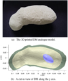 |
Fig. 1 Top: 3D printed detailed model (DM) analog of the relative electric permittivity εr. Bottom: both the analog and the numerical model include the surface layer (mantle), interior part, and the ellipsoidal deep interior void. |
Median structural parameters of the 3D-printed tetrahedral mesh constituting the analog object of this study.
2.2 Permittivity measurements
To obtain refined estimates for the permittivity in the different parts of each analog object, we investigated the bistatic far-field scattering patterns of three 3D-printed test spheres (Eyraud et al. 2015) with volume fraction levels of 66, 90, and 100%. These spheres were based on a 35 mm diameter tetrahedral mesh, whose effective diameter (due to the edge inflation) was found to be 35.5 mm with respect to the asteroid analog (Appendix A). Table 2 shows a priori and a posteriori estimates given by the mixing laws (Sect. 2.1) together with the measured values for the mantle and interior permittivity. The estimates given by the mixing laws are somewhat higher compared to the measured values, which might be partly due to the effect of the fragmented microstructures of the 3D-printed filament resulting from the printing process. The closest match is obtained with MG with a difference of 6% and < 1% to the measured mantle and interior permittivity. In relating the measurements to the effective test sphere diameter 35.5 mm, the permittivity was observed to be 1.5% lower compared to the value obtained for the original 35 mm diameter. Since the effective diameter depending on the modeled detail grows along with the size, with the largest diameter being 35.5 mm, details larger than the test spheres up to the size of the asteroid analog can have 0–1.5% lower permittivity compared to the values in Table 2; the larger the size, the greater the difference (Sorsa et al., in prep.) (Appendix A).
2.3 Laboratory measurements of the wave interaction within the analog
2.3.1 Experimental procedure
The electromagnetic fields scattered by the asteroid analog model were measured using the anechoic chamber of the Centre Commun deRecherches en Microondes (CCRM) in Marseille, France (Fig. 2), which makes it possible to perform measurements at a realistic distance with respect to the diameter of the analog model. Many electromagnetic scattering problems (nm to m wavelengths) can be experimentally simulated with microwaves (cm wavelengths) on a scale of a few centimeters (Geffrin et al. 2012; Vaillon & Geffrin 2014; Barreda et al. 2017; Hettak et al. 2019). Microwave experiments allow us to make accurate measurements of the quantitative complex scattered fields in controlled conditions in order to extract relevant information about the target. Thanks to the centimeter-sized analog targets, such experimental simulations are possible, on the one hand for large objects (tens or hundreds of wavelengths) that involve complex scattering effects and, on the other hand, for nanoscale analog models, which are very difficult to handle, characterize, and control in their original size.
2.3.2 Experiment setup
The measurement distance in the laboratory was set to be 1.85 m, which scales to a 4.83 km distance (orbit), considering the actual size of 25143 Itokawa. To detect the mantle and void inside the analog object, backscattering data were recorded from a direction in which the void is closest to the surface in the horizontal plane intersecting the centre of mass (Fig. 2). The measurements were performed in the quasi-monostatic configuration described in Fig. 2. The source and the receiver were moved together over a given range with respect to both the polar angle ϕ and atsimuth θ of the spherical coordinate system with the center of mass fixed to the origin (Zwillinger 2002), maintaining a constant 12° separation angle between the transmitter and receiver. In both directions, the angular range is 30° and the angular step is 3°, satisfying the Nyquist sampling criterion with respect to the information content of the scattered field (Bucci & Franceschetti 1987). Consequently, both transmitter and receiver positions form a regular 11 × 11 point grid distributed over the surface of the spherical measurement coordinate system. The polarization of the field is linear along the eϕ unit vector, with ϕϕ (vertical) polarization (Fig. 2c).
The fields were measured with continuous waves between 2 and 18 GHz, with a 0.05 GHz frequency step and they were calibrated at each frequency so that the incident electric field at the origin has an amplitude of 1 S m−1 and a null phase. Consequently, the measurements at a given location correspond to a flat-spectrum point source, meaning that any time domain pulse shape can be synthesized based on the measurement data. In this study, we synthesize a Ricker window pulse with the center frequency of 6.00 GHz and two quadrature amplitude modulated Blackman-Harris (BH) window pulses with center frequencies of 10.1 and 12.9 GHz and bandwidths of 5.45 and 5.70 GHz, respectively. Altogether, these cover the investigated frequency range regarding the intensity range from −10 to 0 dB with respect to the pulse amplitude. The limit −10 dB has been chosen to ensure that the signal bandwidths are appropriately contained within the measured frequency range. Both the Ricker and BH windows are frequently used in the processing of the ground-penetrating radar measurements (Priska et al. 2019; Daniels & Institution of Electrical Engineers 2004).
The most significant factors limiting the accuracy of our experimental setup are the ≤ 1 mm positioning and ≤1 degree orientation error allowed by a specifically designed 3D-printed support plate (Fig. 2) and the > 20 dB S∕N of the radar measurement, which was obtained here by evaluating the difference between the measurement and analytically calculated field for a metallic reference sphere. In addition, the accuracy of the final experiment is affected by the modeling approaches utilized in analog preparation and numerical wavefield simulations.
2.3.3 Data
Figure 3 shows the 2D cuts of the radargrams obtained from the measurements considering the entire measurement domain described in Fig. 2 for the two analogs, DM and HM. The radargrams for the DM (top in the Fig. 3) and for the HM (bottom) are rather similar, but for the DM, the signal is denser than in the case of the HM, suggesting the presence of an internal structure. Based on this radargram, we deem that there are no significant hot spots in the data and thereby we choose to investigate the centermost measurement position (Fig. 2) as the primary point of interest.
In order to enable a comparison between the measured and the simulated signal, we divided the temporal domain into mantle I (reflections due to air–mantle and mantle–interior interfaces), void (reflections due to interior–void and void–interior interfaces), mantle II (reflections due to interior–mantle and mantle–air interfaces), and a higher order scattering zone (Fig. 4). These zones, summarized in Table 3, were determined on the basis of a plane wave propagation, as predicted by geometrical optics and considering the different paths involving a single or dual reflection. They contain the effects originating from the subdomains depicted in Fig. 4. The higher order scattering zone involves mainly multipath and multiple scattering effects. As the specific time points of interest, we consider thetwo-way travel-times for the scattering boundaries (1)–(7) described in Table 3. The widths of the zones determined are based on these arrival times, taking into account the duration of the pulse.
Modeled and measured relative permittivity in the DM and HM analog models.
3 Modeling of the wave interaction within the asteroid
To obtain the electromagnetic field scattered by an asteroid analog, we model the electromagnetic interaction with two in-house modeling packages based on (A) frequency and (B) time domain calculations. These numerical simulations are compared with the laboratory measurements in an ideally controlled environment.
3.1 Frequency domain
The interaction between the wave and the asteroid can be modeled in a harmonic domain using the integral formulation of the Maxwell equations. The electric field scattered by an inhomogeneous structure, contained in the spatial domain Ω, is written in the integral form. The scattered field, Es, on the receiver positions, r, included in the domain, Γ, is thus obtained with the observation equation:
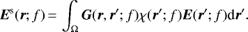 (4)
(4)
Here, E represents the electric field and G the free space dyadic Green’s function between a point r′ in the Ω domain and a point r in the Γ domain, 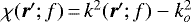 is the contrast term where k(r′; f) is the wavenumberat the point r′ from Ω and ko the wave number in the vacuum.The field E satisfies the following coupling equation:
 (5)
(5)
where Ei(r′; f) is the incident field at point r′ in Ω domain and G(r′, r″; f) the Green’s dyade of the free space between the points r′ and r″ of the Ω area.
Equation (5) is solved numerically using the method of moments (Harrington 1987) and a biconjugated gradient stabilized method (van der Vorst 2003); for more details, see Merchiers et al. (2010). The Toeplitz structure of the dyadic Green function is exploited in this resolution (Barrowes et al. 2001). This improves the computation speed and reduces memory requirements, which is particularly necessary for large objects in relation to the wavelength. Once the scattered field is calculated in the frequency domain, the field in the time domain is obtained in response to a Ricker pulse p(t) using an inverse Fourier transform  as follows:
![\begin{align*} &p(t)\,{=}\,[1-2\pi^2 \,f_{\textrm{c}}^2\,t^2]\exp\left(-\,\pi^2 \,f_{\textrm{c}}^2\,t^2\right),\\ &\mathcal{F}^{-1}[p](f)\,{=}\, C \frac{2}{\sqrt{\pi}}\frac{f^2}{f_{\textrm{c}}^3}\,\exp\left(-\frac{f^2}{f_{\textrm{c}}^2}\right).\end{align*}](/articles/aa/full_html/2020/11/aa38510-20/aa38510-20-eq8.png)
Here, fc is the center frequency of the pulse and C = π3∕2 fc exp(1) is the factor set to normalize the maximum of the Fourier transform of the Ricker pulse to one. In this study, the zero-time reference is taken when the wave is at the source position for all the time domain results.
 |
Fig. 2 Measurement configuration. (a) Complete measurement configuration depicting the transmitter points with solid, black points and the receiver positions in gray circles. (b) Signal path for the centermost transmitter-receiver pair showing a cut-in view through the target. The view is along the z-axis. The source is at the position ϕs = 90°, θs = 174° and the receiver at ϕr = 90°, θr = 186°. (c) Experimental configuration with the angles definition. (d) Photograph of the analog object and the transmitter-receiver pair in the anechoic chamber of the CCRM in Marseille. The transmitter-receiver pair is seen in the background and the 3D-printed support plate applied for positioning is visible under the analog model. |
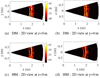 |
Fig. 3 2D view of the 3D radargram obtained considering all the measurements in the configuration described in Fig. 2 for the two analogs, DM and HM. The distance corresponds to the two-way travel after a time-distance conversion considering a propagation in vacuum. The entire frequency band (2–18 GHz) was used for this radargram. The magnitude of the scattered field is given in decibels. |
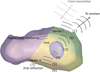 |
Fig. 4 Scattered signal in time domain, which can be identified to have originated from mantle I and II, a void, or higher order scattering zone based on the travel-time of the received signal. The transmitted plane wave is indicated with gray. The wavefronts (1)–(6) correspond to the values given in Table 3. The gray and black arrows indicate the directions of the transmitter and the receiver, respectively. The wavefront (7) corresponds to a round trip inside the analog, starting from reflection number (6). High-order scattering zone includes multi-path and multiple scattering contributions. |
3.2 Time domain
Given a complex-valued permittivity distribution  , the wave can be modeled in the time domain by solving the wave equation for the total field, E, numerically via the following first-order system (Takala et al. 2018a; Sorsa et al. 2020):
![\begin{align*}&\varepsilon'_r \frac{\partial \vec{E}}{\partial t} + \sigma { \vec{E}} - \sum_{i\,{=}\,1}^3 \frac{\partial \vec{F}^{(i)}}{\partial x} + \nabla \, \hbox{Tr} \, [\vec{F}^{(1)} \, \vec{F}^{(2)} \, \vec{F}^{(3)}] \,{=}\, {-}\vec{J}, \! \! \nonumber \\ &\frac{\partial \vec{F}^{(i)}}{\partial t} - \frac{\partial {\vec E}}{\partial x_i} \,{=}\, 0, \end{align*}](/articles/aa/full_html/2020/11/aa38510-20/aa38510-20-eq10.png) (8)
(8)
for i = 1, 2, 3 in the spatio-temporal set [0, T] × Ω ∪ Γ with Tr denoting the trace operator which evaluates the sum of the diagonal entries of its argument matrix and
 (9)
(9)
Denoting the signal frequency as f, the absorption parameter (conductivity) takes the form  . The coordinates are scaled by a spatial scaling factor of s (meters), setting the velocity of the wave in vacuum to one. With this scaling, the time, t, position, r = (x1, x2, x3), absorption σ, and frequency, f, in SI-units can be obtained as
  , sx,
, sx,  , and
, and  , respectively, with ε0 = 8.85 × 10⁻¹² F m−1 denoting the electric permittivity of vacuum and μ0 = 4π × 10−7 H m−1 denoting the magnetic permeability, which is assu- med to be constant in Ω. The right-hand side of Eq. (8) denotes the antenna current density given by J (t, r′) = δp(r)J(t)eA, transmitted at the point, p, in the far-field domain Γ. The time-dependence of the current is J(t). Its position, p, is determined by the Dirac’s delta function, δp(r), and orientation by the vector, eA. By finding the numerical solution, Green’s function, G, can be approximated by [0, T] × Ω ∪ Γ.
The numerical solution of the system (Eq. (8)) within the near-field subdomain [0, T] × Ω can be obtained through the finite element time-domain (FETD) method (Sorsa et al. 2020). The incident and scattered field can be simulated in the far-field subdomain [0, T] × Γ via surface integrals defined on the boundary of Ω (Takala et al. 2018a). An iterative time-domain solver following from the FETD discretization involves sparse matrices which necessitate effective parallel processing for their large size and the need to perform a high number of iteration steps. A state-of-the-art high-performance computing cluster equipped with high-end graphics processing units (GPUs) provides an efficient platform for running such an iteration (Takala et al. 2018a). In this study, the FETD computations were performed using the 32 GB RAM GPUs of the Puhti supercomputer2 (CSC – IT Center for Science Ltd., Finland).
4 Comparison of the numerical simulations both in time and frequency domains versus laboratory measurements
4.1 Cube as a reference case
Since this is the first time that a complex-shaped and comparably large (w.r.t. wavelength) target is measured in this quasi-monostatic configuration, we first validate the present full-wave approach with a cube made of polyethylene. The side length of this cube is equal to 119 mm, corresponding to 1.2 λ and 11 λ with respect to the longest and shortest wavelength (inside the cube) within the investigated frequency band. The permittivity of the cube was found to be equal to εr = 2.35, based on the bistatic far-field scattering patterns of a sphere made of the same material (Eyraud et al. 2015). The comparison between the laboratory measurements and numerical simulations in the frequency domain, presented in Fig. 5, and the corresponding time-domain results (after a Ricker window centered at 6.00 GHz applied to the fields and an inverse Fourier transform) in Fig. 5c validate the configuration for large objects.
4.2 Asteroid analog
The numerical simulations concerning the DM and HM analog models were performed using the measured a posteriori permittivityvalues (Table 2). Table 4 describes the signal properties applied in these simulations for multiple different scales.
4.2.1 Results with the full-wave solver in the frequency domain
The numerical simulations in the frequency domain were perfor- med for theHM and DM analogs. Figure 6 shows a comparison in the frequency domain between the measurement and the numerical simulations in the case of DM and the centermost point. The simulated field is very close to the experimental one below the frequency of 6.00 GHz. The differences that appear at around 6 GHz can be due to local inhomogeneities in the permittivity distribution or possible resonance effects related to the homogenization limit of the analog object. This point is detailed in the discussion (Sect. 5). Once the scattered field has been calculated in the frequency domain, it can be obtained in the time domain via the inverse Fourier transform (Eq. (7)). The scattered fields in the time domain, in response to a Ricker pulse with a center frequency of 6.00 GHz, are shown in Figs. 7a and b for DM and HM, respectively. Figure 7c presents the difference between the magnitude of the temporal field in these two cases. Figure 3 shows that disturbances due to echoes other than the analog echo are low as the signal has a significant value only in the time zone corresponding to the target’s response.
In this response zone, the calculated and measured fields are close to each other for both the DM and HM. In order to analyze these in more detail, we used the temporal arrival times (Table 3) expected for a single reflection on each interface (1)–(6) and for a dual reflection on the back interface (7) (in relation to Fig. 4). In Fig. 7, the first peak in both the measurement and the simulation correspond to the reflection between the air–mantle (1) and mantle–interior (2) interface. The ambiguity between these two responses is due to the pulse duration. The peaks corresponding to the reflections by the back of the asteroid, that is, by the interior–mantle (5) and mantle–air (6) interface, are separate and fully visible in the two curves. The distinguishability of the reflections from the void boundaries (3) and (4) is comparably weak. This somewhat counterintuitive finding suggests that the main part of the energy coming from the void does not directly propagate to the receiver. The final peak (7) corresponds to the second reflection due to the mantle–air interface, that is, a doubled two-way path inside the analog; the time interval between (1) and (7) is roughly double the one between (1) and (6) for each analog and for both the measurement and simulation. In the case of the DM (Fig. 7a), the measured and the simulated fields are relatively intense in the higher order scattering zone compared to the case of HM, where the fields are almost zero in this zone proving that the effects of multipath scattering are likely to be significant with the presence of internal heterogeneity(ies) (Fig. 7b). This is obvious when looking at the magnitude of the difference between the fields obtained in these two cases (Fig. 7c). This is expected as the target has a high contrast and has a relatively large diameter corresponding to the wavelength, suggesting that the wave interaction within this kind of target necessitates a full-wave approach akin the one used here, which takes into account all the multiple interactions.
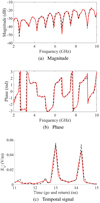 |
Fig. 5 Scattered field of the cube in the configuration described in Fig. 2 for ϕϕ polarization and the central transmitter–receiver position. Measurement is in ( |

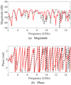 |
Fig. 6 Scattered field for the DM analogs in the configuration described in Fig. 2 for ϕϕ polarization and the central transmitter–receiver position (Fig. 2). Measurement is in ( |
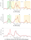 |
Fig. 7 Scattered fields for the DM and the HM analogs in the configuration described in Fig. 2 for ϕϕ polarization and the central transmitter–receiver position (Fig. 2). Measurement is in ( |
4.2.2 Results with the full-wave solver in time domain
Figures 8 and 9 illustrate the measurement and simulation results for the two center frequencies 10.1 and 12.9 GHz of the Blackman-Harris pulse (Table 4). The results are shown for the following three cases: (i) HM data; (ii) DM data; and (iii) the difference between DM and HM data. The approximate of the maximum observed measurement error given by the reference measurement (Sect. 2.3.2) is indicated as a shadowed region around the measurement data, reflecting the credibility of the measurement. As previously, the vertical lines (1)–(7) in the figures indicate the a priori estimated travel-times of the wavefronts scattering from the external and internalboundaries. The measured signal (solid red line) exhibits distinct peaks which localize at the areas where scattering is expected. This effect is clearly visible with the 12.9 GHz center frequency data (the right panel in the Fig. 8), while being somewhat less prominent in the case of the lower center frequency 10.1 GHz (the left panel). Of the two center frequencies, the superior distinguishability of the interior details is obtained with 12.9 GHz which yields clear electrical field amplitude peaks observed in the scattering interfaces in both the measured and the simulated data. For the DM data (the right middle panel), these peaks are localized appropriately in the air-mantle and interior-void-interior interfaces, as expected based on the estimated travel-times (the right panel in the Fig. 8), suggesting that the detail structure inside the asteroid has been detected. The difference curves (the right bottom panel) indicate that the simulated and measured amplitude peaks coincide approximately providing evidence on the detail detection via both the experimental and computational methods.
The comparison between the simulated and measured HM data shows that there are no interior details in HM as the curve lacks most of the peaks observed in the case of the DM. The deviations between the measurement and simulated data can be observed to increase along with the time, which is highlighted in the higher order scattering (strongly non-linear) zone, where the best match corresponds to the DM and 12.9 GHz center frequency.
Figure 9 presents a moving peak S/N between the measurement and FETD simulation for the DM, HM, and DM–HM difference signals. This peak S/N includes the effect of both the measurement and modeling accuracy of which the former is determined by the radar instrument performance (S∕N > 20 dB), positioning and orientation errors (≤1 mm and ≤1 degree, respectively), and the latter one by the accuracy of the numerical FETD simulation and of the modeled permittivity, which can involve deviations of ≤1.5% due to the variation of the edge inflation effect for different surface curvatures (see Appendix A).
Of the two center frequencies, the superior peak S/N is obtained in the case of 12.9 GHz, where the peak S/N for the DM is maintained at or above 10 dB on an interval 11.95–13.4 ns, starting from the mantle I zone, covering the void zone, and the major part of the mantle II zone. Additionally, this level is reached and surpassed in the beginning of the higher order scattering zone. The corresponding peak S/N for the HM is above this level in the mantle II zone, which is obviously due to the backscattering from the exterior surface opposed to the antenna position, but lower in the mantle I and void zones, which can be understood as the mantle and void structure being absent in the HM and, thus, the scattering signal has a lower amplitude over those zones. The peak S/N of the DM–HM difference corresponding to a 12.9 GHz center frequency is above 0 dB otherwise except in the higher order scattering zone. That is, the simulated difference peaks correspond roughly to the measured ones. Because of a lower amplitude, the peak S/N of the difference is lower overall than for either of the DM and HM signals alone.
5 Discussion
This study concerns two asteroid analog models, a homogeneous model (HM) and a detailed model (DM), with the surface shape of the asteroid 25143 Itokawa. DM and HM were investigated through experimental radar measurements and numerical modeling. The permittivity of the interior and mantle were evaluated via an electromagnetic measurement of spherical sample objects. The results we obtained arein a good agreement with the estimates given by the classical mixing models, in particular, the Maxwell Garnett formula. The frequency modeling results show that there is an appropriate match between the measured and simulated fields electric fields in the frequency domain, in both amplitude and phase, up to a frequency of 6.00 GHz (Fig. 6). Above that, the differences observed between the measured and simulated fields may be due to the local inhomogeneities of the 3D-printed mesh and to the resonances related to the metamaterial structure. Based on a visual inspection of the analog object during the 3D printing process, the tetrahedral mesh structure might deviate slightly in vicinity of the compartment boundaries, which might be reflected in the laboratory measurements. At a 6 GHz frequency, the wavelength in the metamaterial and air (2.7 and 5.0 cm, respectively) correspond to about ten times the average edge width and edge length in the interior compartment of the 3D-printed mesh (2.4 and 4.4 mm, respectively), which might be a potential cause of a resonance. These effects are, nevertheless, not very significant in the analysis of time signals, which confirms that the permittivity values measured for the test spheres match with the direct-path travel-times of the wave within the analog. Namely, by setting the permittivity to the measured value, the measured two-way travel-time of the wave, that is, the arrival time of the signal peaks, can be observed to match with the outcome of the numerical simulation. Similarly, when comparing the simulated and measured signals, the observed total attenuation rate, that is, the total effect of absorption and multiple scattering, matches roughly with the expectation given by the permittivity measurement. Moreover, the loss tangent ( ) of the 3D-printed structures is about 0.01 which, based on the present knowledge of asteroid materials and minerals, is close to the expected range for a real asteroid corresponding to around 10–20 dB km−1 attenuation at 10 MHz center frequency (Kofman 2012).
The simulated fields are appropriately matched by the laboratory measurements, verifying that it is possible to distinguish the structural details as separate reflections dominated by the ones from the surface facing and opposing the radar antennae. With respect to frequency-domain modeling (6 GHz center frequency), the time domain results match very well with the laboratory measurements even in the high-order scattering zone. We find a clear difference between the DM and HM analogs in both numerical simulations and laboratory measurements in this high-order scattering zone and also in the mantle I and mantle II zones. With regard to the modeling in the time domain and with a higher center frequency (10.1 and 12.9 GHz), this difference also appears in the void zone, where direct scattering by the void is observed in the case of the DM. It is obvious that the temporal resolution increases with the bandwidth but also that the scattered field depends on the parameters of the applied signal. We regard this as an expected result because of the complexity and non-linearity of the scattering phenomena. For the complexity of the current wave propagation problem, the present frequency and time domain approach constitute two alternative strategies to simulating the signal. We leave a more profound comparison of these methods to a future work.
Full-wave approaches complement other methods developed to calculate the interaction of waves with a target of this size and which are based on optical physics, such as the ray-tracing technique (Ciarletti et al. 2015) and solvers based on physical optics (Berquin et al. 2015). The latter methods do not require the solution of the rigorous diffraction problem and are generally less expensive in terms of computational requirements but, on the other hand, they do not allow for a full reconstruction of the signal. The present strategy for modeling the full wavefield is all the more important since the higher order scattering effects, that is, multi-path and multiple scattering effects are likely to be significant (see for example Fig. 7). In addition, depending on the target geometry and pulse duration, the scattered wavefronts are likely to overlap and involve indirect propagation effects, implying that the full-wave approaches, which take these effects into account appropriately, are fully justified and may even be necessary in order to optimize the outcome of the structural analysis, in particular, as the interior details were observed to affect the higher order scattering wavefronts in this study.
In our earlier studies which focused on simulated measurements (Sorsa et al. 2019; Takala et al. 2018a), a peak S/N of around 10 dB has been found sufficient for finding a reconstruction of the interior structures. The peak S/N analysis of the present experimental study shows that in the case of the DM analog with internal details, this accuracy can be reached and even surpassed in mantle I, void and mantle II zone which correspond to the direct scattering originating from the mantle and void compartment. Together these results suggest that the structural details inside the DM analog object, that is, the surface layer and void, can be distinguished based on the experimental measurement data. Achieving a comparable accuracy with in situ measurements might be possible when assuming that the positioning accuracy is similar, that is, with a ≤ 1 degree angle error (for the potential effect of the orientation inaccuracy, see Takala et al. 2018b) and ≤ 1 mm position error in the analog scale (≤2.6 m scaled to the actual size of 25143 Itokawa). Namely, comparing the S/N of the laboratory measurement (Sect. 2.3.2) to the peak S/Ns observed, it is obvious that the measurement noise is low compared to the errors related to the experimental setup and modeling. Furthermore, our earlier estimates for 1 AU distance from the Sun suggest that the possible measurement errors due to the Galactic noise and the radiation by the Sun will remain at a sufficiently low level with respect to observing the interior structures (Takala et al. 2018a; Sorsa et al. 2019). In particular, their effect can be shrunk via repetitive measurements. Regarding the literature about the signal quality and noise, our present assumptions match also with the general knowledge of the ground-penetrating radar (Daniels & Institution of Electrical Engineers 2004), and by the successful CONSERT measurement (Kofman et al. 2015).
Since the required density of the spatial discretization and, thereby, the computational cost of the simulation increases along with the signal frequency, the applicability of actual target sizes and signal frequencies might still be a computational challenge regarding real in-situ planetary radar measurements. With the current model parameters and asteroid model, we are able to simulate the wave propagation at least up to a target diameter of 264 m at 10 MHz center frequency a bandwidth of 4.42 MHz, which might be sufficient for a real mission configuration (Binzel & Kofman 2005; Kofman 2012; Herique et al. 2018). Furthermore, based on our preliminary numerical experiments, the computing platforms utilized in this study, that is, the 32 GB RAM GPUs of the Puhti supercomputer and the 128 2 TB RAM symmetricalmultiprocessing CPU cores of the Mesocentre AMU, will allow us to expand the target diameter to at least to 480 m or, alternatively, the center frequency to 20 MHz. Considering the potential mission relevance of these numbers, for example, the 163-m moon of the asteroid 65803 Didymos which is the target of the HERA mission fallsinto these limits (Michel et al. 2018). Also, larger asteroids can be considered, the maximum size being dependent on the computing platform’s performance. Targets that do not fit into the memory available can be modeled by restricting the wave simulation process into a subdomain. If needed, such a restriction could be done based on the present principles to divide the scattering processes into lower and higher order scattering zones.
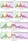 |
Fig. 8 Comparison of the between the measurements and finite element time-domain (FETD) simulation data for the center frequency of 10.1 and 12.9 GHz and ϕϕ polarizationat the central transmitter–receiver position. The solid red and dashed black curve depict the measured and simulated signals, respectively. The shadowed region around the measured signal (red) shows the approximate of the maximum observed error in the reference measurement (Sect. 2.3.2) indicating the credibility of the measurement. The results for the (i) HM and (ii) DM analogs are shown in the top and middle panels, respectively. Bottom panel: (iii) difference between the DM and HM data (Sim. = Simulated, Meas. = Measured). The vertical lines (1)–(7) depict the a priori estimated travel-times (Table 3) of the wavefronts scattering from the surface, mantle, and void matching roughly with the peaks of the measured field and the simulated DM data. These peaks are emphasized in the difference data. Of the center frequencies 10.1 and 12.9 GHz, the latter one yields a superior match between the measured and simulated data. |
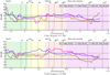 |
Fig. 9 Moving peak S/N between the measurement and FETD simulation for the DM (dashed blue), HM (solid purple), and DM–HM difference (solid brown) signal. Here, the mean power of the simulated signal is normalized to that of the measured one and the length of the moving window is 0.5 ns. Of the center frequencies, 10.1 and 12.9 GHz, the superior overall level is obtained in the latter case, where the peak S/N for DM is maintained over 10 dB (horizontal dashed line) on the interval 11.95–13.4 ns starting in the Mantle I zone, continuing through the void zone almost to the end of the mantle II zone. |
6 Conclusion
The results of this study, obtained in microwave-range laboratory experiments and computer simulations with an analog model based on the shape of the asteroid 25143 Itokawa as a target, suggest that full-wave modeling is a valid approach for investigating the interior structure of asteroids based on radar measurements in both the frequency and time domains. Comparing the present results to earlier numerical simulation studies suggests that a high enough peak S/N can be obtained for the direct scattering from the mantle and void structures, that is, in mantle I, void and mantle II zones. Our results underline that due to the complexity of the scattered wavefield, full-wave modeling might be essential for optimizing the outcome of in situ measurements which are potentially sparse in space missions. Namely, it distinguishes the overlapping direct and indirect wavefronts scattering from different parts of the target and, thereby, allows for the detection of otherwise weakly detectable internal details. For this capability, we are also able to predict multiple scattered and multi-path wavefronts (i.e., data corresponding to higher order scattering zone) which can potentially be utilized in the observation of the interior structures. As the present experiment setup and permittivity modeling approach are applicable with various measurement configurations, asteroid shapes, and interior structures, they can potentially be applied in the examination of subsequent asteroid models in the future.
Acknowledgement
The authors acknowledge the opportunity provided by the Centre Commun de Ressources en Microonde to use its fully equipped anechoic chamber and the Mesocentre of Aix-Marseille University for its support for these numerical simulations. L.-I.S., M.T. and S.P. were supported by the Centre of Excellence in Inverse Modelling and Imaging (Academy of Finland 2018-2025). L.-I.S. was also supported by an Emil Aaltonen Foundation research grant for young researchers. L.-I.S. and S.P. acknowledge CSC – IT Center for Science Ltd., for providing computing services on the Puhti supercomputer. Premix Oy is acknowledged for providing support for the permittivity-controlled 3D printable filament materials.
Appendix A Effect of edge inflation
The volumetric filling and permittivity of the analog objects is controlled by inflating the edges of the tetrahedral mesh. This edge inflation process slightly affects the details of the modeled geometry. Given a meshed detail with a closed surface, this effect can be measured through the ratio ν of the total material Mtotal forming the detail and the proportion enclosed by it Menclosed. This ratio depends on the mesh properties, but is independent of the inflated edge width, which can be observed based on the following definition:
 (A.1)
(A.1)
Here, 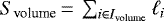 and
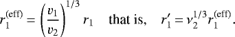
and 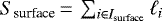 denote the total sum of the edge length. or equivalently that of the inflated edge volume evaluated over the volume of the detail Ivolume, including the surface, and over its surface Isurface, respectively.As the inflated surface edges are symmetrically distributed on both sides of the surface, Ssurface∕2 gives the proportion outside the surface. Assuming that the radius of curvature for the detail is r in the original mesh, it will have the radius r′ = ν1∕3r in the inflated one inflation with 1∕3 following from the conversion between volumetric and one-dimensional scaling. If ν1 and ν2 correspond to some details (1) and (2) with non-inflated and inflated radii of curvature r1, r2 and
  ,
,  , respectively, then the imaginary effective radius
  for which level of inflation with respect to
  is that of r2 with respect to
  detail (2) is defined by:
 (A.2)
(A.2)
Here, detail (1) can be interpreted as a test sphere which we utilize to measure the reference permittivity value of a permittivity layer and (2) as a detail within the asteroid analog model, whose permittivity is to be modeled. Since the tetrahedron size is kept constant, v decreases as the volume of the detail grows. Namely, the total number of tetrahedra grows compared to the number on the surface. Therefore, the larger the detail (2) compared to the test sphere (1) the greater the effective radius  . This means that larger details, that is, those parts of the asteroid analog model with a relatively low surface curvature, will correspond to a slightly larger size, less dense structure, and a lower permittivity value compared to the actual sphere.
References
- Abell, P., Vilas, F., Jarvis, K., Gaffey, M., & Kelley, M. 2006, Lunar and Planetary Science XXXVII [Google Scholar]
- Barreda, A., Saleh, H., Litman, A., Gonzalez, F., & Geffrin, J.-M. 2017, Nat. Commun., 8, 13910 [CrossRef] [Google Scholar]
- Barrowes, B. E., Teixeira, L. F., & Kong, J. A. 2001, Microw. Opt. Technol. Lett., 31, 28 [CrossRef] [Google Scholar]
- Berquin, Y., Herique, A., Kofman, W., & Heggy, E. 2015, Radio Sci., 50, 1097 [CrossRef] [Google Scholar]
- Binzel, R. P., & Kofman, W. 2005, CR Phys., 6, 321 [NASA ADS] [CrossRef] [Google Scholar]
- Birchak, J. R., Gardner, C. G., Hipp, J. E., & Victor, J. M. 1974, Proc. IEEE, 62, 93 [CrossRef] [Google Scholar]
- Bucci, O., & Franceschetti, G. 1987, IEEE Trans. Antennas Propag, 35, 1445 [CrossRef] [Google Scholar]
- Carry, B. 2012, Planet. Space Sci., 73, 98 [NASA ADS] [CrossRef] [Google Scholar]
- Cheng, A. F., Rivkin, A. S., Michel, P., et al. 2018, Planet. Space Sci., 157, 104 [NASA ADS] [CrossRef] [Google Scholar]
- Ciarletti, V., Levasseur-Regourd, A. C., Lasue, J., et al. 2015, A&A, 583, A40 [NASA ADS] [CrossRef] [EDP Sciences] [Google Scholar]
- Daniels, D., & Institution of Electrical Engineers. 2004, Ground Penetrating Radar, Ground Penetrating Radar No. nid. 1 (Institution of Engineering and Technology) [Google Scholar]
- Desch, S. 2007, ApJ, 671, 878 [NASA ADS] [CrossRef] [Google Scholar]
- Eyraud, C., Geffrin, J.-M., Litman, A., & Tortel, H. 2015, IEEE Antennas Wirel. Propag. Lett., 14, 309 [CrossRef] [Google Scholar]
- Eyraud, C., Herique, A., Geffrin, J.-M., & Kofman, W. 2018, Adv. Space Res., 62, 1977 [CrossRef] [Google Scholar]
- Eyraud, C., Saleh, H., & Geffrin, J.-M. 2019, J. Opt. Soc. Am. A, 36, 234 [CrossRef] [Google Scholar]
- Fujiwara, A., Kawaguchi, J., Yeomans, D., et al. 2006, Science, 312, 1330 [NASA ADS] [CrossRef] [PubMed] [Google Scholar]
- Geffrin, J., Garcıa-Camara, B., Gomez-Medina, R., et al. 2012, Nat. Commun., 3, 1171 [CrossRef] [Google Scholar]
- Gomes, R., Levison, H. F., Tsiganis, K., & Morbidelli, A. 2005, Nature, 435, 466 [NASA ADS] [CrossRef] [PubMed] [Google Scholar]
- Harrington, R. 1987, J. Electromagn. Waves Appl., 3, 1 [CrossRef] [Google Scholar]
- Hayabusa Project Science Data Archive. 2007, Itokawa shape model, https://darts.isas.jaxa.jp/planet/project/hayabusa/shape.pl, accessed 4 November, 2019 [Google Scholar]
- Herique, A., Gilchrist, J., Kofman, W., & Klinger, J. 2002, Planet. Space Sci., 50, 857 [CrossRef] [Google Scholar]
- Hérique, A., Kofman, W., Beck, P., et al. 2016, MNRAS, 462 [Google Scholar]
- Herique, A., Agnus, B., Asphaug, E., et al. 2018, Adv. Space Res., 62, 2141 [CrossRef] [Google Scholar]
- Hérique, A., Plettemeier, D., Lange, C., et al. 2019, Acta Astron., 156, 317 [CrossRef] [Google Scholar]
- Hettak, L., Saleh, H., Dahon, C., et al. 2019, IEEE Geosci. Remote Sens. Lett., 17, 933 [CrossRef] [Google Scholar]
- Jutzi, M., & Benz, W. 2017, A&A, 597, A62 [NASA ADS] [CrossRef] [EDP Sciences] [Google Scholar]
- Kawaguchi, J., Fujiwara, A., & Uesugi, T. 2008, Acta Astron., 62, 639 [CrossRef] [Google Scholar]
- Kofman, W. 2012, in 2012 19th IEEE International Conference on Microwaves, Radar & Wireless Communications, 2, 409 [Google Scholar]
- Kofman, W., Herique, A., Goutail, J.-P., et al. 2007, Space Sci. Rev., 128, 413 [NASA ADS] [CrossRef] [Google Scholar]
- Kofman, W., Herique, A., Barbin, Y., et al. 2015, Science, 349, aab0639 [Google Scholar]
- Merchiers, O., Eyraud, C., Geffrin, J.-M., et al. 2010, Opt. Express, 18, 2056 [NASA ADS] [CrossRef] [Google Scholar]
- Michel, P., Kueppers, M., Sierks, H., et al. 2018, Ad. Space Res., 62, 2261 [NASA ADS] [CrossRef] [Google Scholar]
- Morbidelli, A., Levison, H. F., Tsiganis, K., & Gomes, R. 2005, Nature, 435, 462 [NASA ADS] [CrossRef] [PubMed] [Google Scholar]
- Nakamura, T., Noguchi, T., Tanaka, M., et al. 2011, Science, 333, 1121 [Google Scholar]
- Priska, A., Parnadi, W. W., & Parnadi, R. G. 2016 2019 in, IOP Conf. Ser. Earth Environ. Sci., 318, 012028 [CrossRef] [Google Scholar]
- Saleh, H., Tortel, H., Leroux, C., et al. 2020, IEEE Trans. Antennas Propog., in press [Google Scholar]
- Sihvola, A., Nyfors, E., & Tiuri, M. 1985, J. Glaciol., 31, 163 [CrossRef] [Google Scholar]
- Sorsa, L.-I., Takala, M., Bambach, P., et al. 2019, ApJ, 872, 44 [CrossRef] [Google Scholar]
- Sorsa, L.-I., Takala, M., Eyraud, C., & Pursiainen, S. 2020, IEEE Trans. Comput. Imag., 6, 579 [CrossRef] [Google Scholar]
- Takala, M., Bambach, P., Deller, J., et al. 2018a, IEEE Trans. Aerospace Electron. Syst., 55, 1683 [CrossRef] [Google Scholar]
- Takala, M., Us, D., & Pursiainen, S. 2018b, IEEE Trans. Comput. Imag., 4, 228 [CrossRef] [Google Scholar]
- Tsiganis, K., Gomes, R., Morbidelli, A., & Levison, H. F. 2005, Nature, 435, 459 [NASA ADS] [CrossRef] [PubMed] [Google Scholar]
- Vaillon, R., & Geffrin, J.-M. 2014, J. Quant. Spectr. Rad. Transf., 146, 100 [CrossRef] [Google Scholar]
- van der Vorst, H. A. 2003, Iterative Krylov Methods for Large Linear Systems (Cambridge University Press) [CrossRef] [Google Scholar]
- Zwillinger, D. 2002, CRC Standard Mathematical Tables and Formulae, Chapman and Hall/CRC: 31st revised edition [CrossRef] [Google Scholar]
All Tables
Median structural parameters of the 3D-printed tetrahedral mesh constituting the analog object of this study.
All Figures
|
Fig. 1 Top: 3D printed detailed model (DM) analog of the relative electric permittivity εr. Bottom: both the analog and the numerical model include the surface layer (mantle), interior part, and the ellipsoidal deep interior void. |
| In the text | |
|
Fig. 2 Measurement configuration. (a) Complete measurement configuration depicting the transmitter points with solid, black points and the receiver positions in gray circles. (b) Signal path for the centermost transmitter-receiver pair showing a cut-in view through the target. The view is along the z-axis. The source is at the position ϕs = 90°, θs = 174° and the receiver at ϕr = 90°, θr = 186°. (c) Experimental configuration with the angles definition. (d) Photograph of the analog object and the transmitter-receiver pair in the anechoic chamber of the CCRM in Marseille. The transmitter-receiver pair is seen in the background and the 3D-printed support plate applied for positioning is visible under the analog model. |
| In the text | |
|
Fig. 3 2D view of the 3D radargram obtained considering all the measurements in the configuration described in Fig. 2 for the two analogs, DM and HM. The distance corresponds to the two-way travel after a time-distance conversion considering a propagation in vacuum. The entire frequency band (2–18 GHz) was used for this radargram. The magnitude of the scattered field is given in decibels. |
| In the text | |
|
Fig. 4 Scattered signal in time domain, which can be identified to have originated from mantle I and II, a void, or higher order scattering zone based on the travel-time of the received signal. The transmitted plane wave is indicated with gray. The wavefronts (1)–(6) correspond to the values given in Table 3. The gray and black arrows indicate the directions of the transmitter and the receiver, respectively. The wavefront (7) corresponds to a round trip inside the analog, starting from reflection number (6). High-order scattering zone includes multi-path and multiple scattering contributions. |
| In the text | |
|
Fig. 5 Scattered field of the cube in the configuration described in Fig. 2 for ϕϕ polarization and the central transmitter–receiver position. Measurement is in ( |
| In the text | |
|
Fig. 6 Scattered field for the DM analogs in the configuration described in Fig. 2 for ϕϕ polarization and the central transmitter–receiver position (Fig. 2). Measurement is in ( |
| In the text | |
|
Fig. 7 Scattered fields for the DM and the HM analogs in the configuration described in Fig. 2 for ϕϕ polarization and the central transmitter–receiver position (Fig. 2). Measurement is in ( |
| In the text | |
|
Fig. 8 Comparison of the between the measurements and finite element time-domain (FETD) simulation data for the center frequency of 10.1 and 12.9 GHz and ϕϕ polarizationat the central transmitter–receiver position. The solid red and dashed black curve depict the measured and simulated signals, respectively. The shadowed region around the measured signal (red) shows the approximate of the maximum observed error in the reference measurement (Sect. 2.3.2) indicating the credibility of the measurement. The results for the (i) HM and (ii) DM analogs are shown in the top and middle panels, respectively. Bottom panel: (iii) difference between the DM and HM data (Sim. = Simulated, Meas. = Measured). The vertical lines (1)–(7) depict the a priori estimated travel-times (Table 3) of the wavefronts scattering from the surface, mantle, and void matching roughly with the peaks of the measured field and the simulated DM data. These peaks are emphasized in the difference data. Of the center frequencies 10.1 and 12.9 GHz, the latter one yields a superior match between the measured and simulated data. |
| In the text | |
|
Fig. 9 Moving peak S/N between the measurement and FETD simulation for the DM (dashed blue), HM (solid purple), and DM–HM difference (solid brown) signal. Here, the mean power of the simulated signal is normalized to that of the measured one and the length of the moving window is 0.5 ns. Of the center frequencies, 10.1 and 12.9 GHz, the superior overall level is obtained in the latter case, where the peak S/N for DM is maintained over 10 dB (horizontal dashed line) on the interval 11.95–13.4 ns starting in the Mantle I zone, continuing through the void zone almost to the end of the mantle II zone. |
| In the text | |
Current usage metrics show cumulative count of Article Views (full-text article views including HTML views, PDF and ePub downloads, according to the available data) and Abstracts Views on Vision4Press platform.
Data correspond to usage on the plateform after 2015. The current usage metrics is available 48-96 hours after online publication and is updated daily on week days.
Initial download of the metrics may take a while.