| Issue |
A&A
Volume 687, July 2024
|
|
|---|---|---|
| Article Number | A145 | |
| Number of page(s) | 15 | |
| Section | Planets and planetary systems | |
| DOI | https://doi.org/10.1051/0004-6361/202449690 | |
| Published online | 05 July 2024 | |
A high-precision 3D reconstruction method for the internal structure of small Solar System bodies
Research Center of Satellite Technology, Harbin Institute of Technology,
Harbin,
PR China
e-mail: This email address is being protected from spambots. You need JavaScript enabled to view it.
; This email address is being protected from spambots. You need JavaScript enabled to view it.
Received:
21
February
2024
Accepted:
2
May
2024
Abstract
Context. Small Solar System bodies (SSSBs) hold crucial information for understanding the formation and evolution of the Solar System. However, due to their considerable distance, small size, fast rotation, and a lack of prior information, the detection of these celestial bodies, especially their internal structures, faces numerous challenges.
Aims. We explore whether the 3D structure of SSSBs can be reconstructed using monostatic radar. We investigated a more convenient observation mode and addressed the issue of the poor imaging quality of internal structures within existing imaging algorithms.
Methods. Our study focused on a high-precision 3D imaging method for the internal structure of SSSBs based on radar signals. First, we considered a flyby observation mode that uses the spinning characteristics of the target for global observations, and we set up a scaled-down experimental system in the laboratory to simulate this observation mode. Next, we constructed a 3D printed physical surface model based on the shape of the asteroid 162173 Ryugu. We filled it with sand and inserted a small bottle containing different materials separately to construct two distinct layered analogs. The analogs were employed in laboratory measurements to acquire radar echoes, which were then inverted using both a classic back-projection (BP) algorithm and a modified multilayer back-projection (MLBP) method.
Results. The results shown that the 3D surface structure of the target can be reconstructed well through the BP and MLBP algorithms. The MLBP algorithm exhibits a higher reconstruction accuracy for internal structures. Moreover, compared to the BP method, the MLBP method is less sensitive to the quality of echo signals, resulting in a relatively stable imaging performance.
Conclusions. Our findings reveal that observing and reconstructing the high-precision structure of SSSBs is feasible through our proposed method. The observation mode, experimental setup, and analog modeling approach are widely applicable and can be applied in future research on the detection of SSSBs with more diverse and complex structures.
Key words: scattering / waves / techniques: image processing / minor planets, asteroids: general / planets and satellites: interiors
© The Authors 2024
 Open Access article, published by EDP Sciences, under the terms of the Creative Commons Attribution License (https://creativecommons.org/licenses/by/4.0), which permits unrestricted use, distribution, and reproduction in any medium, provided the original work is properly cited.
This article is published in open access under the Subscribe to Open model. This email address is being protected from spambots. You need JavaScript enabled to view it. to support open access publication.
1 Introduction
Exploring the internal structure of small Solar System bodies (SSSBs) is a crucial scientific question for understanding the formation and evolution of the Solar System. In recent years, with the continuous improvement of aerospace technology, space detection has become an integral part of the exploration of SSSBs. Radar technology, with advantages such as high speed, nondestructiveness, and high resolution, is currently the most mature remote-sensing method for measuring the interior of celestial bodies, and it holds significant research potential. The European Space Agency’s (ESA) Rosetta mission, launched in 2004, marked the initial endeavor to employ a radar instrument for exploring SSSBs. The mission used bistatic radar (Barbin et al. 1999; Kofman et al. 2007) that was carried by both the orbiter and lander. It aimed to investigate the internal structure of Comet 67P/Churyumov-Gerasimenko (Safaeinili et al. 2002) and has yielded rich scientific results (Kofman et al. 2015). The HERA mission, scheduled for launch in 2024 as part of an asteroid deflection initiative, plans to deploy two 6U CubeSats carrying low-frequency radar (Herique et al. 2019) to investigate the surface characteristics and internal structure of the binary asteroid 65803 Didymos system (Bambach et al. 2018). Through the promotion of these projects, scientific research on the use of radar methods to detect the interior of small bodies has gradually increased in recent years. The research involves forward-modeling methods, inverse algorithms, numerical simulations, measurement systems, and other aspects.
In recent years, numerous studies on radar-imaging inversion methods have been conducted. Currently, two general categories of 3D imaging algorithms are suitable for reconstructing the interior of small bodies. The first category comprises full-wave inversion techniques, which developed from time-domain seismic imaging (Tarantola & Valette 1982; Tarantola 1986), and have been extensively developed in the field of geophysics (Boonyasiriwat et al. 2009). This approach inverts the 3D dielectric properties of an object by using the complete information (including time, amplitude, and phase) of the signal and matching forward-model predictions to measurements. Most of the techniques for seismic waveform inversion can be applied to electromagnetic wave inversion (van den Berg et al. 1999; Haynes et al. 2012). Given its capability to obtain relatively rich internal physical property information and its advantages in high resolution, full-wave electromagnetic inversion is considered a promising method for the interior exploration of SSSBs and has been studied by scientists from various countries (Takala et al. 2018; Sava & Asphaug 2018; Sorsa et al. 2019, 2021; Eyraud et al. 2020; Deng et al. 2022). In recent years, driven by research trends such as big data and artificial intelligence, technologies such as deep learning have also been applied to optimize algorithms in the field of full-wave inversion (He & Wang 2021). However, these studies did not fully take into account the multiple coupling phenomena, and due to issues such as high computational intensity, sensitivity to initial models, and the nonuniqueness problem, this approach still has many limitations and challenges in practical applications. The second category comprises free-space methods (Haynes et al. 2021), primarily referring to radar tomography (Knaell & Cardillo 1995) and synthetic aperture radar (SAR) imaging. Dufaure et al. (2023) conducted laboratory measurements to indicate that the structure of asteroid analogs can be reconstructed using a back-propagation and pseudo-inverse tomography algorithm. These technologies have applications in Earth imaging and mapping (Wu et al. 2011), as well as in the exploration of celestial bodies such as the Moon and other major planets such as Mars (Simpson et al. 2006; Nozette et al. 2010; Neish et al. 2011; Li et al. 2020). SAR has significant advantages in terms of cost and deployment. Although it has some limitations in terms of the comprehensiveness of information compared to full-wave inversion methods, its ease of analysis, high resolution, and imaging efficiency mean that it performs exceptionally well in high-precision structure reconstruction and real-time on-orbit processing. Therefore, the SAR method shows strong prospects for application in future missions for the internal exploration of SSSBs.
The back-projection (BP) algorithm is one of the classic SAR imaging algorithms that performs imaging by back-projecting scattered echoes into the image domain. Arumugam et al. (2018) explored the inversion method for 2D comet interior imaging using the BP algorithm and ray-bending correction (Wu et al. 2011). Gassot et al. (2021) used a point target simulation to evaluate the internal imaging performance of the frequency domain back-projection algorithm (FDBP) and compressive sensing (CS) algorithm for SSSBs. However, in the conventional SAR imaging method, the variation in the speed of radar signals during propagation inside the target is not taken into account. Consequently, the imaging results of the internal structure may exhibit significant errors compared to the actual target. To address these issues, we propose a modified 3D MLBP method that incorporates the surface structure model of the target for phase compensation. In this study, we explore a readily attainable and cost-effective flyby observation mode, using the spinning characteristics of the target for global observations. Subsequently, a laboratory experimental setup was established based on this observation mode, and two different layered asteroid analogs were constructed for laboratory measurements. The reconstruction of 3D images for the analogs was accomplished using both BP and MLBP methods. Several quantitative quality measures were employed to assess and quantify the performance of the proposed imaging methods, indicating their effectiveness.
The rest of this paper is organized as follows: Sect. 2 introduces the observation mode. In Sect. 3, we present and describe the asteroid analogs, the experimental setup, and the measurement methods. Section 4 analyzes the wave propagation and explains the imaging methods. The imaging results are presented and discussed in Sect. 5. We conclude in Sect. 6.
2 Observation mode
The space exploration of SSSBs generally involves several key stages, including interstellar transfer, approach, flyby, hover, and landing (Li et al. 2019). Remote-sensing detection typically takes place from the approach to the landing stage. When addressing smaller bodies such as Asteroid 2016HO3 (the focus of the Zhenghe Mission detection target, Zhang et al. 2019), which has a diameter smaller than 100 meters, the natural orbiting period for the detector becomes excessively long. In this situation, the radar motion relative to the target is dominated by the rotation of the asteroid itself. In this paper, we consider an observation mode in which the spacecraft performs a flyby parallel to the rotation axis of the target. Simultaneously, the spacecraft maintains the orientation of the radar antenna toward the target center, ensuring that the target remains continuously within the beam of the antenna throughout the observation. In this process, we leverage the rotational characteristics of the target to gather radar echoes from multiple perspectives. The schematic illustration of the observation scenario is shown in Fig. 1a, the radar trajectory in an inertial frame can be approximated as a straight line, and for small bodies with short rotation periods, a single slow flyby corresponds to multiple rotations in general. Therefore, the relative motion trajectory between the detector and the target can be equivalent to an ascending spiral, as shown in Fig. 1b. This is the most easily achievable observation mode and eliminates the need for excessive fuel consumption to alter the detector motion status for revisiting the target. This results in a more expedient, cost-effective observation mode with lower requirements for the control system.
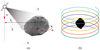 |
Fig. 1 Schematic diagram of the observation mode. (a) Observation scenarios. (b) Equivalent geometric of the observation mode. |
3 Laboratory experiments with the asteroid analog
3.1 Asteroid analog
In this study, we made two scaled-down asteroid analogs for radar measurements. Referring to the research of Eyraud et al. (2020), we considered the analog model to consist of three parts: an external mantle, an interior with homogeneous material, and a deep interior anomaly.
We prepared the external mantle analog using a 3D printed surface model (Fig. 2g) based on the shape of asteroid 162173 Ryugu (Fig. 2e, explored by the space mission Hayabusa2, Watanabe et al. 2019). The material of the external surface model was ABS plastic with a nominal relative permittivity of 3.3~4.2 at 1KHz, and we measured its relative permittivity using the waveguide method at 10−15 GHz to be approximately εr ≈ 2.7. The measured values are somewhat lower than the nominal value, which might be partly due to the effect of the material microstructures during the 3D printing process and to the difference in frequencies. The model was hollow, with a thickness of 3 mm. The envelope dimension of the external surface model was 0.3044 × 0.3045 × 0.2574 m3. To facilitate installation and positional calibration on the experimental platform, the bottom of the model was processed into a flat surface, and orthogonal grooves were carved to define the coordinate system and origin, as shown in Fig. 2g. This ensured that the position remained unchanged with each installation.
The surface model can be filled with various materials to simulate SSSBs with different compositions. In this study, we filled the surface model with quartz sand, which has a relative permittivity of  and a particle size of 0.6 ~ 1 mm, to represent the interior part. Subsequently, a bottle filled with different materials was inserted into the sand separately to simulate two distinct deep interior anomalies, as illustrated in Fig. 2h. One anomaly was filled with electrolyte water
  and is referred to as the liquid anomaly model (LAM). The other was filled with air
  and is referred to as the air anomaly model (AAM). The coordinates of the center point of the deep interior anomaly are (−0.008 m, 0.047m, 0.021m). The specific dimensions and relative positional relations of the analog are depicted in Figs. 2a−d.
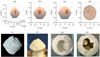 |
Fig. 2 Analog of asteroid 162173 Ryugu. (a−d) 3D structure of the analog. (e) Grayscale photography of asteroid 162173 Ryugu, (f) Ryugu analog in the anechoic chamber. (g) Surface model of the analog. (h) Layered structure of the analog. |
3.2 Laboratory measurements
We measured the electromagnetic fields scattered by the analogs in an anechoic chamber, as shown in Fig. 3. This enabled us to accurately measure the quantitative complex scattered fields within a controlled environment, allowing for the experimental simulation of numerous electromagnetic scattering problems on a scale of a few centimeters. The experiments were conducted within the frequency band of 12−24 GHz. In Table 1, we list the parameter correspondence between the scaled and real measurement scenarios. In the laboratory, using a frequency of 18 GHz to measure a target with a diameter of 0.3 m can be equivalent to using a frequency of 6 MHz to measure a small body with a diameter of about one kilometer (e.g., asteroid Ryugu, which has an approximate diameter of 980 m). Similarly, it is equivalent to using a frequency of 10 MHz to measure a small body with a diameter of about 500 m (e.g., asteroid Itokawa, which has an approximate diameter of 540 m), and to using a frequency of 100 MHz to measure a small body with a diameter of about 50 m (e.g., asteroid 2016 HO3, with a diameter smaller than 100 m).
We implemented an experimental setup to conduct measurements based on the flyby observation mode introduced in Sect. 2. The block diagram of the experimental setup is depicted in Fig. 4, encompassing the primary components of antennas, the horizontal turntable, the linear slide table, the tilting angle table, the data acquisition equipment, and the control terminal. The horizontal turntable has a rotation range of 0−360°, the linear slide table has a sliding range of 0−1.5 mm, and the tilting angle table has a rotational angle range of −45° to + 45°. The analog was placed on the horizontal turntable, simulating the rotational motion characteristics. The receiving and transmitting antennas were assembled with the linear slide table and tilting angle table to simulate the linear trajectory of the detector when it flies over the target and to control the direction of the antenna beam. This combination of movements enables the radar to observe the analog from various directions, achieving an observation mode similar to that shown in Fig. 1b.
The coordinate system is defined as shown in Fig. 5; we use this coordinate system throughout the rest of the paper. The rotation axis of the horizontal turntable is along the Z-axis, and the direction of the line connecting the slide table and the horizontal turntable is the X-axis. Here, H1 = 0.99 m, Rc = 1.49 m, D = 1.5 m, and D0 = 0.255 m. The receiving antenna and the transmitting antenna are two identical broadband horns with linear polarization, mounted in parallel on the tilting angle table, with a center horizontal distance of 52 mm. In this experiment, we adopted a step-by-step measurement mode. The schematic diagram showing the distribution of measurement points is presented in Fig. 6. The transmitting−receiving antenna pair started at ɀ = −0.735 m and slid along the +z direction with a step length of 0.023 m, totaling 64 observation positions. At each observation position, the target rotated for one complete revolution, with 512 samples taken per cycle. Each pulse consisted of 400 sampling points. The total amount of data obtained from one complete measurement process is 400 × 512 × 64.
The accuracy of the experimental setup depends on the control error of the moving components and on the accuracy of the position calibration. The horizontal turntable and tilting angle table can provide a degree orientation error smaller than 0. 01°, and the positioning error of the linear slide table is smaller than 0.05 mm. The position measurement error of the system is smaller than 1 mm.
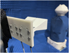 |
Fig. 3 Photograph of the analog object and the transmitter-receiver pair in the anechoic chamber. |
Sizes and scaling of the analogs with respect to the real scale measurements.
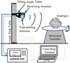 |
Fig. 4 Schematic block diagram of the experimental system. |
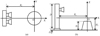 |
Fig. 5 Definition of the coordinate system of the experimental system. (a) Front view. (b) Side view. |
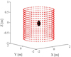 |
Fig. 6 Scheme of the measurement point distribution. |
4 Imaging method
4.1 Propagation of the radar signals
The target can be simplified as a triangulated surface model consisting of N facets. In a monostatic configuration, this is an option to simplify the wave propagation model, as shown in Fig. 7. Geometrical optics and ray-tracing were employed to model the incoming signal and the propagation of fields within the target. Figure 7b illustrates the propagation path of the radar signal for a facet on the target.
The total electric field received at the radar detector is the sum of the surface response Esurf (rn) and the internal subsurface response Esub>(rn),
 (1)
(1)
Esurf(rn) and Esub(rn) can be derived through the reflection Stratton-Chu integral (Hsu & Barakat 1994) and Snell’s law. The detailed calculation process can be found in Fa et al. (2009); Gerekos et al. (2018).
To achieve sufficient range resolution and transmitted power, we used linear frequency modulation (LFM) chirp signals (Curlander & McDonough 1991) as the emitted signal,
![Mathematical equation: $s(t) = W(t)\exp \left[ {j2\pi \left( {{f_c}t + {1 \over 2}\hat \gamma {t^2}} \right)} \right]\quad t \in \left[ { - {T_p}/2,{T_p}/2} \right],$](/articles/aa/full_html/2024/07/aa49690-24/aa49690-24-eq5.png) (2)
(2)
where fc and Tp denote the carrier frequency and the pulse width of the emitted signal, respectively.  refers to the chirp acceleration term of an LFM waveform, and W(t) is the corresponding envelope in the range direction, usually approximated as a rectangular pulse. The time-dependent emitted field at the emission point is thus given by
 (3)
(3)
where τη represents the delay with which the reflected signal arrives back at the antenna. In subsequent processing, we neglected the multiple scattering. Then for the surface echoes, this delay is simply the two-way signal travel time in vacuum τη = 2|P0 - P1 |/c. For the echoes from the subsurface layer, however, the delay is given by
![Mathematical equation: ${\tau _n} = {1 \over c}\left[ {\left| {{P_1} - {P_0}} \right| + \left| {{P_0} - {P_3}} \right|} \right] + {1 \over {{v_g}}}\left[ {\left| {{P_2} - {P_1}} \right| + \left| {{P_3} - {P_2}} \right|} \right],$](/articles/aa/full_html/2024/07/aa49690-24/aa49690-24-eq8.png) (4)
(4)
where  , c is the speed of light,
  is the relative permittivity of the interior material of the target in the subsequent imaging processing, and
  is assumed to be a known quantity.
  , which is the relative permittivity of vacuum.
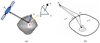 |
Fig. 7 Simplified wave propagation model. (a) Monostatic configuration. (b) Propagation path of the radar signal. |
4.2 Back-projection algorithm
The back-projection (BP) algorithm, a classical SAR timedomain imaging algorithm (Soumekh 1999), involves back-projecting the received signals onto an image plane and reconstructing the scene by assigning pixel values based on the accumulated radar echoes. In the processing step, the position of each data point is determined by its phase information, as the phase directly relates to the wave travel-time, and hence, to distance. By summing and accumulating all the back-projected data, the final image is formed. Here, waves with matching phases are enhanced, while unrelated waves (noise or signals from other directions) are suppressed due to phase mismatch. Therefore, we did not consider the effects of polarization.
Let Rn(tm) represent the distance between the radar and a point n on the target at the instantaneous moment tm. By performing range compression on the time-dependent emitted field E(t) given by Eq. (3), we obtain
![Mathematical equation: $E\left( {\tau ,{t_m}} \right) = {\mathop{\rm sinc}\nolimits} \left[ {B\left( {\tau - {{2{R_n}\left( {{t_m}} \right)} \over c}} \right)} \right] \cdot \exp \left[ { - jk{R_n}\left( {{t_m}} \right)} \right],$](/articles/aa/full_html/2024/07/aa49690-24/aa49690-24-eq13.png) (5)
(5)
where B denotes the bandwidth of the radar signal, and k denotes the vacuum wavenumber.
We defined a 3D image grid composed of resolution cells and aligned the image grid with the flight trajectory of the radar detector in a common coordinate system. For each radar echo, we calculated the geometric delay and determined the corresponding location on the image grid. We accumulated the radar echoes at their respective locations on the grid. Subsequently, the imaging process can be expressed as
![Mathematical equation: ${I^{(p)}} = \int_{{t_m}} E \left( {\tau ,{t_m}} \right)\exp \left[ {jk{R_p}\left( {{t_m}} \right)} \right]{\rm{d}}{t_m},$](/articles/aa/full_html/2024/07/aa49690-24/aa49690-24-eq14.png) (6)
(6)
where I(p) represents the imaging results in resolution cell P, and Rp(tm) is the distance between the radar antenna and the resolution cell P at tm.
4.3 Multilayer back-projection algorithm
The BP method can reconstruct high-precision images of the target surface structures, but it does not account for signal refraction. When addressing interior imaging issues, the mapping positions of internal echo data in the image grid may differ from the actual positions. Consequently, the imaging results may exhibit significant positioning errors compared to the actual internal structure. Therefore, we investigated an MLBP imaging method based on the reconstructed surface structures to enhance the reconstruction accuracy of the internal structures.
The detailed flowchart of the proposed MLBP method is shown in Fig. 8. First, the BP method was used for the 3D imaging to reconstruct the surface triangulated model of the target, denoted as EM. We assumed that the model EM consists of N triangular facets, and we denote the normal vector of each facet as  We considered EM as the boundary and generated the imaging resolution domain M according to the Jordan curve theorem (Berg et al. 1975; Li & Wang 2017). We ensured that all resolution cells were located inside the boundary, satisfying M ∈ EM.
The mapping relation between radar echo and imaging resolution domain is shown in Fig. 9. If the radar received a total of Q pulses, the distance at the qth sampling position Q(q) between the radar antennas and the imaging resolution cell M(m) can be approximated as
 (7)
(7)
where
 (8)
(8)
 (9)
(9)
Nq represents the effective coverage area of the radar antenna beam on the target surface at the sampling position Q(q), and  is the angle between the incident wave vector and the normal vector of surface facet ɀ(n). The theoretical value of θs should be π/2, but in practical situations, the echo amplitude decreases rapidly with increasing incident angle θi, and its contribution to the imaging can be negligible after a certain range is exceeded. Therefore, θs can be appropriately reduced to improve the computational efficiency.
We summed the contributions of all echoes to generate the final pixel value. The reconstructed resolution cell m can then be discretely represented as
![Mathematical equation: ${I^{(m)}} = \sum\limits_{q = 1}^Q s (\tau ,q)\exp [jkR(q,m)].$](/articles/aa/full_html/2024/07/aa49690-24/aa49690-24-eq20.png) (10)
(10)
Application of the above operations to all cells in M results in the complete reconstructed image.
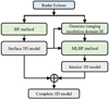 |
Fig. 8 Flowchart of the proposed 3D MLBP method. |
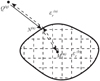 |
Fig. 9 Schematic diagram of the imaging resolution domain mapping of the MLBP imaging algorithm. |
5 Imaging results
In this section, we apply the BP and MLBP algorithms to perform 3D imaging for the LAM and AAM experimental data, respectively. To facilitate the observational and quantitative comparison, we normalized the images to ensure that the amplitude range of the each image was between 0 and 1.
5.1 Quantitative quality measures
To quantitatively assess the imaging results, we evaluated the following quantitative quality measures between the exact and reconstructed images: the root mean square error (RMSE), the structural similarity (SSIM), the peak signal-to-noise ratio (PSNR), the positioning error (PE), and the relative overlap (RO).
The PSNR and RMSE are standard and widely used quantitative quality measures for image evaluation. The PSNR measures the ratio of the peak signal power to the power of the noise or distortion. It is typically expressed in decibels (dB), with higher values indicating a smaller difference between the original and reconstructed signals, implying a better quality. The RMSE is calculated by taking the square root of the average of the squared differences between estimated and actual values. Lower values indicate a better reconstructed performance. The SSIM (Wang et al. 2004) index is a metric used to measure the similarity between two images. It takes into account luminance, contrast, and structure, providing a comprehensive assessment of the image quality. The SSIM index ranges from 0 to 1, where 1 indicates perfect similarity.
To evaluate the quality of particular areas of the image, we divided the reconstructed image into two parts: Rint, representing the internal area of the analog, and Rext, representing the surface and external area of the analog. The entire reconstructed image is Rall = Rint ∪ Rext. Similarly, the external set Iext, the internal set Iint, and the entire theoretical image of the analog satisfy Iall = Iint ∪ Iext. The particular quantitative quality measures [·]α (α = int,ext,or all) were calculated using the corresponding set of the images. For example, PSNRall = psnr(Iall, Rall), SSIMint = ssim(Iint, Rint), and RMSEext = rmse(Iext, Rext).
Subsequently, we obtained 3D point clouds from the reconstructed images using an amplitude threshold, as shown in Figs. 11, A.5, and A.3. The point clouds set PCα can be obtained as follows:
 (11)
(11)
We used PE and RO to evaluate the quality of the point clouds. When we assume that the number of points in the set is N, the distance between each point and the triangulated surface model of the theoretical analog is defined as distance deviation, denoted as  . PE is then defined as the root mean square difference of the distance deviation,
 (12)
(12)
Relative overlap refers to the extent to which two objects or regions overlap relative to their individual sizes. It is defined in Sorsa et al. (2020); Dufaure et al. (2023) as the percentage
 (13)
(13)
Here, RCα is the point cloud set generated from Rα, and SCα is the theoretical point cloud set sampled from the analog model Ια. For discrete point sets, ‘Area(•)’ represents the number of points in the set. We employed the range resolution (∆r = c/2B) as the decision threshold. Points with distances smaller than ∆r between the two sets were classified as overlapping points, whereas points with distances greater than ∆r were classified as error points. RO provides a measure of the similarity or agreement between two segmented objects. A higher value indicates a greater degree of overlap.
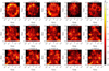 |
Fig. 10 Slices of the amplitude of the reconstructed 3D images using the BP method for the AAM analog. The slices in the first row are parallel to the XOY plane, those in the second row are parallel to the XOZ plane, and those in the third row are parallel to the YOZ plane. |
5.2 Imaging results of the BP algorithm
In this section, we present and analyze the reconstructed results of the BP method as described in Sect. 4.2. Figure 10 shows the 2D slices of the reconstructions for the AAM analogs, and Fig. A.1 shows the reconstructed 2D slices of the LAM analog, along with the comparison results against the true model contours. Three planes were selected at different positions along each direction of the X-, Y-, and Z-axes for the observation. The slices in the first row were parallel to the XOY plane, those in the second row were parallel to the XOZ plane, and those in the last row were parallel to the YOZ plane. The white-line plots correspond to the theoretical analogs in Fig. A.1. The external shape of the two analogs reconstructed by the BP algorithm closely matches the theoretical contour, but the internal part is reconstructed at a position that is slightly out of line with the theoretical contour. In the slices of the XOZ and YOZ planes in Figs. 10 and A.1, a noticeable trapezoidal contour can be observed in the region from ɀ = −0.2 m to ɀ = −0.1 m. This is formed by the reflection of the pedestal in the laboratory. In subsequent processing, we manually removed this portion of the images.
In order to carry out a more rigorous comparison, the quantitative quality measures introduced in Sect. 5.1 were evaluated. The computed results of PSNR, SSIM, and RMSE for the reconstructed 3D images compared to the theoretical analog models can be found in Table 2. Due to the identical structure and material of the external surface in the LAM and AAM analogs, the PSNRext, SSIMext, and RMSEext are nearly the same for the two imaging results with the BP method. The SSIM and RMSE of the external results are both superior to the internal results. This is consistent with the observations in the 2D slices and matches the theoretical expectations. Because the permittivity of the interior anomaly in the LAM analog is significantly greater than that of the AAM analog, the reflectivity for radar signals is correspondingly stronger. Consequently, it is evident that the quantitative quality measures for the LAM analog are superior to those of the AAM analog in the internal results obtained with the two imaging methods.
Subsequently, we extracted points from the reconstructed 3D image whose amplitudes exceeded a certain threshold, recorded their 3D coordinates and amplitudes, and generated the point cloud diagram. Figures A.3 and 11 display the point clouds of the LAM and AAM analogs obtained from the 3D images reconstructed by the BP algorithm using thresholds of −6dB, −8dB, and −10dB. The results of RO and PE for the reconstructed point clouds compared to the theoretical analog model can be found in Tables 3 and 4. The lower the threshold, the more points in the point cloud, resulting in a more complete reconstruction of the target structure, and the RO of the internal and external structures continuously increases. However, simultaneously, this also introduces more noise, leading to greater positioning errors. When the RO is the same, PEext is consistently smaller than PEint, indicating a higher accuracy in reconstructing the external structure compared to the internal structure.
Then, we used the point cloud data of AAM, generated with the threshold of −9 dB, to reconstruct the 3D polygon mesh of the external shape. First, we used the open-source Iso2Mesh library (Tran et al. 2020) to generate a 3D closed surface, as shown in Fig. 12a. Due to the large number of polygon mesh faces obtained and their uneven distribution, we employed Poisson disk sampling to repartition the mesh, resulting in a uniformly subdivided mesh model, as illustrated in Fig. 12b. We calculated the distance between the centroid of each face in the reconstructed mesh model and the triangulated surface of the actual analog model, and defined the root mean square of all these distances as the reconstruction error. The reconstruction error for the 3D mesh model is 0.0163 m, with a relative overlap (RO) of 62.23%. The same process was applied to the point cloud data of LAM, yielding the reconstruction result shown in Fig. A.2. The reconstruction error for the LAM mesh model is 0.0163 m, with an RO of 58.24%.
Quantitative results of the 3D reconstructed images with the BP method.
Quantitative results of the 3D reconstructed point clouds for the LAM analog with the BP method.
Quantitative results of the 3D reconstructed point clouds for the AAM analog with the BP method.
5.3 Imaging results of the MLBP algorithm
In this section, we present and compare the MLBP method, as introduced in Sect. 4.3, for the internal reconstruction with the reconstructed external model (REM) and the actual external model (AEM). The REM is depicted in Figs. 12b and A.2b, and the AEM is shown in Fig. 2a. All of the external models used in this section contained 1500 triangular faces. Figures 13 and A.4 display the reconstructed slices of the internal part of the AAM and LAM analogs, respectively. Rows (a) shows the results of the BP method, and rows (c) and (d) show the results of the MLBP method with the AEM and REM. The three slices in each row are orthogonal to the X-, Y-, and Z-axes. They pass through the center of the interior anomaly (ɀ = 0.02 m, x = −0.008 m, y = 0.047 m). Since the MLBP algorithm only reconstructs the internal region of the analog, the imaging results of the BP algorithm were also limited to the internal region for the sake of comparison. The white-line plots correspond to the theoretical analogs.
In order to establish a uniform comparison interval, each internal region was defined by the shape of the actual object.
The results show that the interior structures of the MLBP method are reconstructed with a more appropriate location and shape than the results of the BP method. Both AEM and REM can be used to obtain well-reconstructed results. Due to the difference in reflectivity of the interior anomalies, the brightness of the internal shape in the reconstructed images of the AAM are noticeably lower than that of the reconstructed images of the LAM. Tables 5 and 6 show the quantitative results of the internal reconstructed results. For the LAM analog, the internal reconstruction results of the MLBP method with the AEM show improvements of 9.20, 1.40, and 23.90% in PSNR, SSIM, and RMSE, respectively, compared to those obtained directly using the BP algorithm for the reconstruction. With the REM, the improvements are 4, 0.2 and 14.5%. For the AAM analog, the improvements for the internal reconstructions with the MLBP AEM are 23.35, 1.83, and 45.00%, and with the REM, they are 20.7, 1.1, and 41.2%. The MLBP method is clearly better applicable. Additionally, the internal imaging results reconstructed using the REM have a slightly worse PSNR, SSIM, and RMSE compared to those using the AEM. This is because the errors in the REM results stem from the accumulation of model reconstruction errors and resolution errors, whereas the AEM results are due to the errors in system positioning and resolution, and the system positioning error is much smaller than the reconstruction error. This indicates that the accuracy of the external model reconstruction can indeed affect the quality of the internal imaging to a certain extent.
Figure A.5 displays the internal part of the reconstructed point clouds for the two analogs using the BP and MLBP methods. The yellow part is the theoretical structure of the interior anomaly, and the blue points are the reconstructed point clouds. The results obtained by the MLBP method (Figs. A.5b,c,e and f) match the theoretical structure better than those obtained by the BP method (Figs. A.5a and d). Quantitative comparisons of these reconstructed results are presented in Tables 7 and 8. When the RO is similar, the PE of the reconstructed results for the MLBP method is significantly better than that of the BP method. For the AAM analog, the PE of the internally reconstructed part by the BP method remains around 0.06 m, indicating a lower accuracy compared to the imaging results of the LAM analog.
Quantitative results of the 3D reconstructed images of the LAM analog.
Quantitative results of the 3D reconstructed images of the AAM analog.
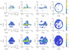 |
Fig. 11 Reconstructed point cloud of the target using BP algorithm for the AAM analog. (a) Threshold = −6 dB. (b) Threshold = −8 dB. (c) Threshold = −10 dB. |
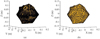 |
Fig. 12 Reconstructed 3D external shape of the AAM. (a) Reconstruction results with the Iso2Mesh library. (b) Reconstruction results after Poisson disk sampling. |
Quantitative results for the 3D point clouds of the internal structure in the LAM analog.
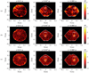 |
Fig. 13 Slices of the reconstructed images of the internal region of the target using the BP and MLBP methods for the AAM analog. The line plot corresponds to the theoretical analog. (a) BP method. (b) MLBP method with the AEM. (c) MLBP method with the REM. |
Quantitative results for the 3D point clouds of the internal structure in the AAM analog.
 |
Fig. 14 Surface models with different accuracies for the MLBP method. From left to right, the numbers of facets are 5000, 3000, 1500, 1000, 500, and 250. |
Quantitative quality of the images reconstructed with different surface models.
5.4 Effect of the external model
As the MLBP method relies on the target surface structure, the accuracy and computing time are directly influenced by the input 3D surface grid model. To analyze the influence of surface models on the MLBP imaging performance, we resampled the actual external model to generate triangulated models with total facet numbers of 5000, 3000, 1500, 1000, 500, and 250, as illustrated in Fig. 14. In order to ensure the reliability of the comparison results, all simulation programs in this group of experiments were run on the same workstation. MLBP imaging was conducted on the measured data from the AAM analog, and the quantitative quality measures for these reconstructions are presented in Table 9. Each PE was calculated under a similar RO of approximately 96% to facilitate comparison.
The quantitative analysis results from Table 9 indicate that the more accurate the external model, the better the reconstruction of internal structures. When the generated point clouds have the same RO, a finer model leads to smaller PE for the point clouds. However, as the number of model faces increases, the extent of this improvement gradually decreases. When employing imaging using the surface model with 3000 faces, the PE of 0.0127 m is nearly close to the theoretical resolution of 0.0125 m. Subsequently, a continuously increasing model accuracy does not necessarily result in a corresponding improvement in the precision of the reconstructed images. Moreover, an excessive increase in the number of overlays may introduce more noise and may consequently cause a decline in reconstruction accuracy. An increase in the number of faces also means an increase in computing time. Therefore, the accuracy of the surface model for the MLBP method should be chosen as a trade-off between resolution requirements and computational resources.
6 Conclusions
We built an experimental setup based on the slow flyby observation mode and conducted multiple measurements to analyze the inversion method for small Solar System bodies. Two asteroid analogs were employed to investigate 3D imaging methods with radar signal. These two analogs share identical external shapes and compositional components. One analog contained a liquid deep interior anomaly, and the other featured an air anomaly. The BP algorithm was employed to reconstruct the 3D external structure of the target. A modified MLBP method was proposed to enhance the reconstruction performance of the internal structures. Additionally, several quantitative quality measures were applied to assess and quantify the similarity between the reconstructed and the actual structure of the analogs.
The results indicate that the external and internal boundaries of these analogs can be effectively reconstructed. In the imaging results of the BP algorithm, the external boundaries of the analogs are clearly observed, and the internal structure is also visible, but the positions differ more strongly than for the external results. Based on the 3D imaging results of the BP method, we reconstructed the 3D polygon mesh of the external shape of the analog. The MLBP method improved the results of the internal structure reconstruction, exhibiting significant enhancements in both image quality and positional accuracy. The AEM and REM are both capable of producing well-reconstructed results. Furthermore, it shows good applicability for echo signals with relatively poor quality. Additionally, we analyzed the influence of the surface model accuracy on the internal imaging results for the MLBP method. The results indicate that the more detailed the surface model, the better the reconstructed internal image, but it also increases the computation time. The proposed method has demonstrated its capability for the 3D reconstruction of asteroid targets and can also be applied to reconstruct the internal structures of SSSBs. Given the adaptability of our experimental setup and analog modeling approach to various measurement configurations, asteroid shapes, and interior structures, they hold potential for examining SSSBs in the future.
Acknowledgements
This work received support from the Research Center of Satellite Technology, Harbin Institute of Technology. The authors express gratitude for insightful discussions with their colleagues. Appreciation is extended to the editor and anonymous reviewers for their dedicated time and efforts. The authors sincerely value the constructive comments and advice provided to enhance the manuscript in alignment with its objectives.
Appendix A Complementary figures for the imaging results
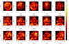 |
Fig. A. 1 Slices of the amplitude of the reconstructed 3D images using the BP method for the LAM analog. The line plot corresponds to the theoretical analog. The slices in the first row are parallel to the XOY plane, those in the second row are parallel to the XOZ plane, and those in the third row are parallel to the YOZ plane. |
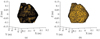 |
Fig. A. 2 Reconstructed 3D external shape of the LAM. (a) Reconstruction results with the Iso2Mesh library. (b) Reconstruction results after Poisson disk sampling. |
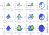 |
Fig. A. 3 Reconstructed point cloud of the target using the BP algorithm for the LAM analog. (a) Threshold = −6 dB. (b) Threshold = −8 dB. (c) Threshold = −10 dB. |
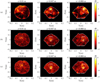 |
Fig. A. 4 Slices of the reconstructed images of internal region of the target using the BP and MLBP methods for the LAM analog. The line plot corresponds to the theoretical analog. (a) BP method. (b) MLBP method with AEM. (c) MLBP method with REM. |
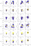 |
Fig. A. 5 Reconstructed point clouds of the internal structures of the target. The threshold is −6dB for all images. (a) BP method for the LAM analog. (b) MLBP method for the LAM analog with AEM. (c) MLBP method for the LAM analog with REM. (d) BP method for the AAM analog. (e) MLBP method for the AAM analog with AEM. (e) MLBP method for the AAM analog with REM. |
References
- Arumugam, D. D., Gim, Y., Heggy, E., & Wu, X. 2018, IEEE ISAP & USNC/URSI National Radio Science Meeting, Boston, American, 1795 [Google Scholar]
- Bambach, P., Deller, J., Vilenius, E., et al. 2018, Adv. Space Res., 62, 3357 [NASA ADS] [CrossRef] [Google Scholar]
- Barbin, Y., Kofman, W., Nielsen, E., et al. 1999, Adv. Space Res., 24, 1115 [NASA ADS] [CrossRef] [Google Scholar]
- Berg, G., Julian, W., Mines, R., & Richman, F. 1975, Rocky Mt. J. Math, 5, 225 [CrossRef] [Google Scholar]
- Boonyasiriwat, C., Valasek, P., Routh, P., et al. 2009, Geophysics, 74, WCC59 [NASA ADS] [CrossRef] [Google Scholar]
- Curlander, J. C., & McDonough, R. N. 1991, Synthetic Aperture Radar (New York: Wiley), 11 [Google Scholar]
- Deng, J., Kofman, W., Zhu, P., et al. 2022, IEEE Trans. Geosci. Electron., 60, 1 [Google Scholar]
- Dufaure, A., Eyraud, C., Sorsa, L.-I., et al. 2023, A&A, 674, A72 [NASA ADS] [CrossRef] [EDP Sciences] [Google Scholar]
- Eyraud, C., Sorsa, L. I., Geffrin, J. M., et al. 2020, A&A, 643, A68 [NASA ADS] [CrossRef] [EDP Sciences] [Google Scholar]
- Fa, W., Xu, F., & Jin, Y. 2009, Sci. China Ser. F, 52, 559 [CrossRef] [Google Scholar]
- Gassot, O., Herique, A., Fa, W., Du, J., & Kofman, W. 2021, Rad. Sci., 56, 1 [CrossRef] [Google Scholar]
- Gerekos, C., Tamponi, A., Carrer, L., et al. 2018, IEEE Trans. Geosci. Electron., 56, 7388 [Google Scholar]
- Haynes, M., Clarkson, S., & Moghaddam, M. 2012, IEEE Trans. Antennas Propag., 60, 1854 [CrossRef] [Google Scholar]
- Haynes, M. S., Fenni, I., Gim, Y., Kofman, W., & Herique, A. 2021, Adv. Space Res., 68, 3903 [NASA ADS] [CrossRef] [Google Scholar]
- He, Q., & Wang, Y. 2021, Geophysics, 86, V1 [NASA ADS] [CrossRef] [Google Scholar]
- Herique, A., Plettemeier, D., Kofman, W., et al. 2019, Proc. EPSC-DPS Joint Meeting, 13, 807 [NASA ADS] [Google Scholar]
- Hsu, W., & Barakat, R. 1994, J. Opt. Soc. Am. A, 11, 623 [NASA ADS] [CrossRef] [Google Scholar]
- Knaell, K., & Cardillo, G. 1995, IEE Proc.-Radar, Sonar Navigat., 142, 54 [CrossRef] [Google Scholar]
- Kofman, W., Herique, A., Goutail, J. P., et al. 2007, Space Sci. Rev., 128, 413 [CrossRef] [Google Scholar]
- Kofman, W., Herique, A., Barbin, Y., et al. 2015, Science, 349, aab0639 [Google Scholar]
- Li, J., & Wang, W. 2017, Comput. Aided Des., 87, 20 [CrossRef] [Google Scholar]
- Li, X., Qiao, D., Huang, J., Han, H., & Meng, L. 2019, Sci. Sin-Phys. Mech. As., 49, 084508 [NASA ADS] [Google Scholar]
- Li, C., Su, Y., Pettinelli, E., et al. 2020, Sci. Adv., 6, eaay6898 [Google Scholar]
- Neish, C. D., Bussey, D. B. J., & Spudis. 2011, J. Geophys. Res.: Planets, 116, 1005 [CrossRef] [Google Scholar]
- Nozette, S., Spudis, P., Bussey, B., et al. 2010, Space Sci. Rev., 150, 285 [NASA ADS] [CrossRef] [Google Scholar]
- Safaeinili, A., Gulkis, S., Hofstadter, M., & Jordan, R. 2002, Meteorit. Planet. Sci., 37, 1953 [NASA ADS] [CrossRef] [Google Scholar]
- Sava, P., & Asphaug, E. 2018, Adv. Space Res., 61, 2198 [NASA ADS] [CrossRef] [Google Scholar]
- Simpson, R. A., Tyler, G. L., Pätzold, M., & Häusler, B. 2006, J. Geophys. Res. Planets, 111 [CrossRef] [Google Scholar]
- Sorsa, L.-I., Takala, M., Bambach, P., et al. 2019, ApJ, 872, 44 [NASA ADS] [CrossRef] [Google Scholar]
- Sorsa, L.-I., Takala, M., Eyraud, C., & Pursiainen, S. 2020, IEEE Trans. Comput. Imaging, 6, 579 [CrossRef] [Google Scholar]
- Sorsa, L.-I., Pursiainen, S., & Eyraud, C. 2021, A&A, 645, A73 [NASA ADS] [CrossRef] [EDP Sciences] [Google Scholar]
- Soumekh, M. 1999, Synthetic Aperture Radar Signal Processing (New York: Wiley), 7 [Google Scholar]
- Takala, M., Us, D., & Pursiainen, S. 2018, IEEE Trans. Comput. Imaging, 4, 228 [CrossRef] [Google Scholar]
- Tarantola, A. 1986, Geophysics, 51, 1893 [NASA ADS] [CrossRef] [Google Scholar]
- Tarantola, A., & Valette, B. 1982, Rev. Geophys., 20, 219 [NASA ADS] [CrossRef] [Google Scholar]
- Tran, A. P., Yan, S., & Fang, Q. 2020, Neurophotonics, 7, 015008 [CrossRef] [Google Scholar]
- van den Berg, P. M., Van Broekhoven, A., & Abubakar, A. 1999, Inverse Problems, 15, 1325 [NASA ADS] [CrossRef] [Google Scholar]
- Wang, Z., Bovik, A. C., Sheikh, H. R., & Simoncelli, E. P. 2004, IEEE Trans. Image. Process., 13, 600 [CrossRef] [Google Scholar]
- Watanabe, S., Hirabayashi, M., Hirata, N., et al. 2019, Science, 364, 268 [NASA ADS] [Google Scholar]
- Wu, X., Jezek, K. C., Rodriguez, E., et al. 2011, IEEE Trans. Geosci. Electron., 49, 3791 [Google Scholar]
- Zhang, X., Huang, J., Wang, T., & Huo, Z. 2019, Lunar Planet. Sci. Conf., 2132, 1045 [Google Scholar]
All Tables
Quantitative results of the 3D reconstructed point clouds for the LAM analog with the BP method.
Quantitative results of the 3D reconstructed point clouds for the AAM analog with the BP method.
Quantitative results for the 3D point clouds of the internal structure in the LAM analog.
Quantitative results for the 3D point clouds of the internal structure in the AAM analog.
All Figures
|
Fig. 1 Schematic diagram of the observation mode. (a) Observation scenarios. (b) Equivalent geometric of the observation mode. |
| In the text | |
|
Fig. 2 Analog of asteroid 162173 Ryugu. (a−d) 3D structure of the analog. (e) Grayscale photography of asteroid 162173 Ryugu, (f) Ryugu analog in the anechoic chamber. (g) Surface model of the analog. (h) Layered structure of the analog. |
| In the text | |
|
Fig. 3 Photograph of the analog object and the transmitter-receiver pair in the anechoic chamber. |
| In the text | |
|
Fig. 4 Schematic block diagram of the experimental system. |
| In the text | |
|
Fig. 5 Definition of the coordinate system of the experimental system. (a) Front view. (b) Side view. |
| In the text | |
|
Fig. 6 Scheme of the measurement point distribution. |
| In the text | |
|
Fig. 7 Simplified wave propagation model. (a) Monostatic configuration. (b) Propagation path of the radar signal. |
| In the text | |
|
Fig. 8 Flowchart of the proposed 3D MLBP method. |
| In the text | |
|
Fig. 9 Schematic diagram of the imaging resolution domain mapping of the MLBP imaging algorithm. |
| In the text | |
|
Fig. 10 Slices of the amplitude of the reconstructed 3D images using the BP method for the AAM analog. The slices in the first row are parallel to the XOY plane, those in the second row are parallel to the XOZ plane, and those in the third row are parallel to the YOZ plane. |
| In the text | |
|
Fig. 11 Reconstructed point cloud of the target using BP algorithm for the AAM analog. (a) Threshold = −6 dB. (b) Threshold = −8 dB. (c) Threshold = −10 dB. |
| In the text | |
|
Fig. 12 Reconstructed 3D external shape of the AAM. (a) Reconstruction results with the Iso2Mesh library. (b) Reconstruction results after Poisson disk sampling. |
| In the text | |
|
Fig. 13 Slices of the reconstructed images of the internal region of the target using the BP and MLBP methods for the AAM analog. The line plot corresponds to the theoretical analog. (a) BP method. (b) MLBP method with the AEM. (c) MLBP method with the REM. |
| In the text | |
|
Fig. 14 Surface models with different accuracies for the MLBP method. From left to right, the numbers of facets are 5000, 3000, 1500, 1000, 500, and 250. |
| In the text | |
|
Fig. A. 1 Slices of the amplitude of the reconstructed 3D images using the BP method for the LAM analog. The line plot corresponds to the theoretical analog. The slices in the first row are parallel to the XOY plane, those in the second row are parallel to the XOZ plane, and those in the third row are parallel to the YOZ plane. |
| In the text | |
|
Fig. A. 2 Reconstructed 3D external shape of the LAM. (a) Reconstruction results with the Iso2Mesh library. (b) Reconstruction results after Poisson disk sampling. |
| In the text | |
|
Fig. A. 3 Reconstructed point cloud of the target using the BP algorithm for the LAM analog. (a) Threshold = −6 dB. (b) Threshold = −8 dB. (c) Threshold = −10 dB. |
| In the text | |
|
Fig. A. 4 Slices of the reconstructed images of internal region of the target using the BP and MLBP methods for the LAM analog. The line plot corresponds to the theoretical analog. (a) BP method. (b) MLBP method with AEM. (c) MLBP method with REM. |
| In the text | |
|
Fig. A. 5 Reconstructed point clouds of the internal structures of the target. The threshold is −6dB for all images. (a) BP method for the LAM analog. (b) MLBP method for the LAM analog with AEM. (c) MLBP method for the LAM analog with REM. (d) BP method for the AAM analog. (e) MLBP method for the AAM analog with AEM. (e) MLBP method for the AAM analog with REM. |
| In the text | |
Current usage metrics show cumulative count of Article Views (full-text article views including HTML views, PDF and ePub downloads, according to the available data) and Abstracts Views on Vision4Press platform.
Data correspond to usage on the plateform after 2015. The current usage metrics is available 48-96 hours after online publication and is updated daily on week days.
Initial download of the metrics may take a while.