| Issue |
A&A
Volume 645, January 2021
|
|
|---|---|---|
| Article Number | A73 | |
| Number of page(s) | 13 | |
| Section | Planets and planetary systems | |
| DOI | https://doi.org/10.1051/0004-6361/202039380 | |
| Published online | 15 January 2021 | |
Analysis of full microwave propagation and backpropagation for a complex asteroid analogue via single-point quasi-monostatic data
1
Computing Sciences, Tampere University (TAU),
PO Box 692,
33101
Tampere,
Finland
e-mail: This email address is being protected from spambots. You need JavaScript enabled to view it.
2
Aix Marseille Univ., CNRS, Centrale Marseille, Institut Fresnel,
Marseille,
France
Received:
9
September
2020
Accepted:
13
November
2020
Abstract
Context. Information carried by the full wave field is particularly important in applications involving wave propagation, backpropagation, and a sparse distribution of measurement points, such as in tomographic imaging of a small Solar System body.
Aims. With this study, our aim is to support the future mission and experiment design, such as for example ESA’s Hera, by providing a complete mathematical and computational framework for the analysis of structural full-wave radar data obtained for an asteroid analogue model. We analyse the direct propagation and backpropagation of microwaves within a 3D printed analogue in order to distinguish its internal relative permittivity structure.
Methods. We simulate the full-wave interaction between an electromagnetic field and a three-dimensional scattering target with an arbitrary shape and structure. We apply the Born approximation and its backprojection (the adjoint operation) to evaluate and backpropagate the wave interaction at a given point within the target body. As the data modality can have a significant effect on the distinguishability of the internal details, we examine the demodulated wave and the wave amplitude as two alternative data modalities and perform full-wave simulations in frequency and time domain.
Results. The results obtained for a single-point quasi-monostatic measurement configuration show the effect of the direct and higher-order scattering phenomena on both the demodulated and amplitude data. The internal mantle and void of the analogue were found to be detectable based on backpropagated radar fields from this single spatial point, both in the time domain and in the frequency domain approaches, with minor differences due to the applied signal modality.
Conclusions. Our present findings reveal that it is feasible to observe and reconstruct the internal structure of an asteroid via scarce experimental data, and open up new possibilities for the development of advanced space radar applications such as tomography.
Key words: scattering / techniques: image processing / minor planets, asteroids: general
All the authors contributed equally.
© L.-I. Sorsa et al. 2021
 Open Access article, published by EDP Sciences, under the terms of the Creative Commons Attribution License (https://creativecommons.org/licenses/by/4.0), which permits unrestricted use, distribution, and reproduction in any medium, provided the original work is properly cited.
1 Introduction
This article concerns the modelling of full-wave propagation and backpropagation with an asteroid analogue model as the target. The possibilities provided by these techniques continue to expand thanks to the rapidly increasing computing resources which enable modelling of the full wave propagation in an arbitrary domain and at high frequency. Information carried by the full wave field is particularly useful in applications based on sparse distribution of wave transmission and/or measurement points in order to maximise the information content of the eventual measurements. Here, our focus is on potential radar investigations of future space missions (Hérique et al. 2018, 2019; Takala et al. 2018; Sorsa et al. 2019, 2020; Eyraud et al. 2020). Our objective is to provide a complete mathematical and computational framework for the analysis of structural full-wave radar measurements obtained for a structurally complex asteroid analogue model, thereby supporting the related future space mission and laboratory experimental design. In particular, we consider the 3D printed analogue of Eyraud et al. (2020) which is based on the optical high-resolution shape model of asteroid 25143 Itokawa (Fujiwara et al. 2006; Hayabusa Project Science Data Archive 2007). In Eyraud et al. (2020), we investigated this analogue using state-of-the-art laboratory experiments, showing that full wave modelling, which can predict both the direct and higher order scattering effects caused by its complex shape and structure, is needed for this analogue. The analysis presented here constitutes an important feasibility study for the observation of the internal structure of this analogue using data obtained in laboratory-based experiments. Finding a backpropagated reconstruction based on radar data is an ill-posed and ill-conditioned inverse problem (Bertero & Boccacci 1998) meaning that slight errors in the measurement, the numerical model, or the choice of the data modality can have a significant effect on the result. For this reason, we compare several different approaches.
In planetary science (Picardi et al. 2005; Kofman et al. 2007, 2015; Grima et al. 2009; Blair et al. 2017; Haruyama et al. 2017; Kaku et al. 2017), there is a need to detect radiowave scattering from different obstacles and interior structures to maximise the scientific outcome of a space mission. Important goals in this regard are, for example, to distinguish scattering from surface and subsurface obstacles and to determine their relative permittivity in order to infer the structure of the investigated domain. Planetary radar investigations have so far led to important scientific discoveries, such as for example in the exploration of the Moon and Mars in which the mapping of the Lunar lava tubes (Haruyama et al. 2017; Kaku et al. 2017; Blair et al. 2017) and the detection of the Martian water ice (Picardi et al. 2005; Grima et al. 2009) are among the most significant recent findings.
In small-body research, the interior structure of the comet 67P/Churyumov-Gerasimenko was recently investigated by the CONSERT instrument (Kofman et al. 2007, 2015) during ESA’s Rosetta mission. Significant future plans to perform surface-penetrating radar measurements include, for example, the Hera mission which is the European component of the Asteroid Impact and Deflection Assessment (AIDA) mission, a joint effort between ESA and NASA. The primary target of Hera will be the asteroid moon of the binary system of 65803 Didymos. Such future radar investigations will be crucial, as current knowledge of small-body interiors still relies on indirect data, such as for example the outcome of impact simulations and density estimates obtained for binary systems (Vernazza et al. 2020). From the modelling perspective, the planned in situ investigations pose a special challenge because the complex shape and surface structure of a small Solar System body results in various interlaced scattering phenomena which require the application of advanced numerical methodology to achieve the scientific goals. The complexity of the modelling and inversion task is further emphasised by the large size of the target and therefore the large wave field as compared to the wavelength, the restricted bandwidth of the measurement, and the limited number of measurement points.
In this article, we perform a numerical analysis of the full wave interaction between an electromagnetic field transmitted by a microwave radar and a 3D-printed asteroid analogue in both the time and the frequency domain. We analyse the direct and higher-orderscattering effects numerically by examining the effect of the signal frequency and bandwidth on the wave propagation, and the sensitivity of the radar to detect obstacles in different parts of the analogue model. We apply the Born approximation (BA) and its adjoint operation (backprojection) to evaluate and backpropagate the wave interaction at a given point withinthe target body. As the data modality can have a significant effect on the distinguishability of the internal details, we examine thedemodulated wave and the wave amplitude as two different alternative, linearly independent, and complementary signal modalities.
The results obtained for a single-point quasi-monostatic measurement configuration show the effect of the direct and higher-orderscattering phenomena on both the demodulated and amplitude data. The internal mantle and void of the analogue were found to be detectable based on backpropagated radar fields from this single spatial point, which is the minimum signal configuration in the case of a radar space mission, in both the time and the frequency domain approaches, with minor differences due to the applied signal modality. The methodology and findings presented here are crucial for observing and reconstructing the internal structure of an asteroid via experimental data, as suggested earlier in Eyraud et al. (2020), and open up new possibilities for the development of space radar applications, such as for example tomography, where the interior structure of the target is reconstructed using a large set of multi-directional measurements.
This article is structured as follows: in Sect. 2, we briefly review the frequency and time-domain-based approaches to model wave propagation within the analogue. In Sect. 3, we describe the methods for the analysis of the fields, including time–frequency domain analysis, and BA and its backprojection. In Sect. 4, both the asteroid analogue and the radar configuration are detailed. The results are presented in Sect. 5 and discussed in Sect. 6, and our conclusions are presented in Sect. 7.
2 Wave propagation models
We apply two in-house software implementations to obtain the full wave (forward) interaction of an electromagnetic wave with an asteroid analogue. One of these implementations is based on the integral formulation of the Maxwell’s equations with the solution in the frequency domain, and the other one on a local formulation solved in the time domain. The mathematical methodology applied in these forward solvers is briefly described in this section.
2.1 Solution in the frequency domain
2.1.1 Formulation
The volume integral formulation allows us to compute the scattered electric field by an inhomogeneous structure included in the spatial domain Ω, i.e. a structure with a spatially variable relative permittivity εr. At each point r′ in Ω, the relative permittivity can be written as
 (1)
(1)
with εr(r′;f) and  denoting, respectively, the real and the imaginary part of the relative electrical permittivity in Ω domain at the point r′. The scattered field Es on the receiver position r in the Γ domain is obtained via the observation equation
 (2)
(2)
with E representing the total electric field, that is E = Ei + Es, which is the sum of the incident (illuminating) field Ei and the scattered one Es, and G representing the Green’s dyadic function between an r′ point in the Ω domain and an r point in the Γ domain. Here,  is the contrast term with k(r′) denoting the wave number at the point r′ from the Ω zone and k0 is the wave number in the vacuum.
The field E satisfies the following coupling equation:
 (3)
(3)
which we evaluate numerically using the method of moments (Harrington 1987). The linear system is solved using a stabilised biconjugate gradient method (van der Vorst 2003); for more details see Merchiers et al. (2010). The properties of the dyadic Green’s function are exploited in this resolution as explained below.
2.1.2 Computational considerations
The dyadic Green’s function used in these equations corresponds to the free space. This function has a multilevel block-Toeplitz structure. The exploitation of this structure, which is explained in Barrowes et al. (2001), allows one to store only non-redundant elements. This considerably reduces the memory requirement which is particularly necessary for the present application with objects that are very large compared to the wavelength. The use of this multi-level Toeplitz block structure also accelerates matrix-vector multiplications containing the matrix of Green’s dyadic function. It is based on one-dimensional (1D) FFT implementations directly as opposed to 2D and 3D FFTs.
2.2 Solution in the time domain
The wave can be modelled via the following locally defined first-order system of partial differential equations for the total field (Takala et al. 2018; Sorsa et al. 2020):
![Mathematical equation: \begin{align*}&\varepsilon'_{\textrm{r}} \frac{\partial {\textbf{E}}}{\partial t} + \sigma {\textbf{{ E}}} - \sum_{i = 1}^3 \frac{\partial {\textbf{F}}^{(i)}}{\partial x_i} + \nabla \, \hbox{Tr} \, [\textbf{F}^{(1)} \, \textbf{F}^{(2)} \, \textbf{F}^{(3)}] = -\textbf{J}, \nonumber \\ &\frac{\partial {\textbf{F}}^{(i)}}{\partial t} - \frac{\partial {\textbf{E}}}{\partial x_i} = 0, \end{align*}](/articles/aa/full_html/2021/01/aa39380-20/aa39380-20-eq6.png) (4)
(4)
where i = 1, 2, 3 in the spatio-temporal set [0, T] × Ω ∪ Γ, where T denotes the length of the investigated time interval and Tr the trace operator which evaluates the sum of the diagonal entries for its argument matrix. The absorption parameter (conductivity) is of the form  . The right-hand side of Eq. (4) denotes the current density of the antenna given by J (t, r′) = δp(r) J(t) eA and transmitted at p ∈ Γ. The time-dependence of the current is J(t), its position p is determined by the Dirac’s delta function δp(r) and orientation is eA. The near-field numerical solution of the system (4) in [0, T] × Ω is obtained here using the finite element time-domain (FETD) method (Sorsa et al. 2020). The incident and scattered far-field field in [0, T]× Γ follow from Kirchhoff’s surface integrals defined on the boundary of Ω (Takala et al. 2018).
The coordinates are scaled by a spatial scaling factor s (metres). When s = 1 m, the velocity of the wave in vacuum is equal to one. Given s, the time t, position r = (x1, x2, x3), absorption σ, and frequency f in SI-units can be obtained as  , sr,
, sr,  , and
, and  respectively, with the electric permittivity of vacuum being ε0 = 8.85 × 10⁻¹² F/m and the magnetic permeability which is assumed to be constant in Ω being μ0 = 4π × 10−7 H/m.
2.2.1 Quadratic amplitude modulation
In our FETD simulation, the signal propagated is assumed to be a quadrature amplitude modulated (QAM) Blackman-Harris (BH) window function. Quadrature amplitude modulation allows amplitude-preserving modulation and demodulation of the signal and is therefore suitable for the radar signal transmission and measurement. In QAM, a two-component signal sf = [sf,I, sf,Q] with an amplitude of  is carried by an in-phase and quadrature component sf,I and sf,Q, which are modulated by a carrier wave with a frequency f and have a mutual phase difference of π∕2. Here these components are defined as
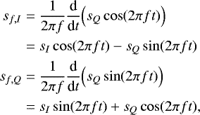 (5)
(5)
where sI defines the in-phase component and
 (6)
(6)
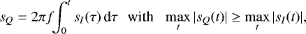
the quadrature component of the original unmodulated signal s = [sI, sQ]. In this study, sQ is set to be the BH window and sI its time derivative according to (6). The amplitude of s is equal to that of sf, i.e.
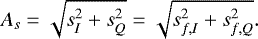 (7)
(7)
Given the modulated signal components sf,I, the original signal s = [sI, sQ] = [sI, sQ] can be obtained via a demodulation process, where the phase ϕ of the carrier is sought by maximising the function
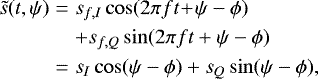 (8)
(8)
at the point tmax = argmaxt|sQ(t)| with respect to the phase of the demodulation ψ, that is,  . The in-phase and quadrature component of s can be obtained as
  and
and  . Namely, the equation sI (tmax) = 0, which follows from the definition (6) of sQ(t), implies that ϕ maximises the second (sinus) term of (8). In other words, the amplitude As and |sQ | are maximised at the same time point, where As = |sQ| and sI vanishes.
2.2.2 Computational considerations
An iterative time-domain solver following from the FETD discretisation necessitates effective parallel processing, as each iteration step involves large, sparse matrices following from the spatial finite element discretisation. A sufficiently efficient platform for running such an iteration is provided by a state-of-the-art high-performance computing cluster equipped with high-end graphics computing units (GPUs) (Takala et al. 2018). In this study, the FETD computations were performed using the 32 GB RAM GPUs of the Puhti supercomputer1, CSC – IT Center for Science, Finland.
3 Numerical analysis of the wave interaction
3.1 Time–frequency analysis
To perform a time–frequency analysis, that is, a multi-band analysis over a wide frequency range, the scattered field in the time domain in response to a signal pulse s can be expressed as
 ](t) ,\end{equation*}](/articles/aa/full_html/2021/01/aa39380-20/aa39380-20-eq19.png) (9)
(9)
with  and
and  denoting the Fourier transform and its inverse. Here, we use the Ricker pulse
![Mathematical equation: \begin{align*} &s(t)=[1-2\pi^2 \,f_{\textrm{c}}^2\,t^2]\exp\left(-\,\pi^2 \,f_{\textrm{c}}^2\,t^2\right),\\ &\mathcal{F}[s](f)= \frac{ 2\pi \, f^2}{f_{\textrm{c}}^2}\,\exp\left(1-\frac{f^2}{f_{\textrm{c}}^2} \right), \end{align*}](/articles/aa/full_html/2021/01/aa39380-20/aa39380-20-eq22.png)
where fc is the centre frequency of the pulse. Once the scattered field has been calculated in the frequency domain, it can be obtained in the time domain using an inverse Fourier transform.
\, \mathbf{E}_s (\mathbf{r}; f) \exp\left(j\,2\,\pi\,f\,t\right)\, \textrm{d}f ,\end{equation*}](/articles/aa/full_html/2021/01/aa39380-20/aa39380-20-eq23.png) (12)
(12)
with fmin and fmax denoting the minimum and maximum frequencies of the band.
3.2 Bornapproximation
To analyse the point-wise scattering effects, we apply the BA presented in Takala et al. (2018) and Sorsa et al. (2020), which gives an estimate for the effect of a single-point permittivity perturbation on the wave propagation within the target object. A BA can be formed via Tikhonov regularised deconvolution between (1) a wave u(t) originating from the transmission antenna and (2) a reciprocal of a wave h(t) emitted by the receiving antenna. The Tikhonov regularised deconvolution (Sorsa et al. 2020) can be evaluated at the point of scattering as given by
 \, \mathcal{F}[u](f) }{\mathcal{F}[s](f) + \nu} \right](t), \end{equation*}](/articles/aa/full_html/2021/01/aa39380-20/aa39380-20-eq24.png) (13)
(13)
where BA is denoted by d, the signal transmitted by s, and the constant regularisation parameter by ν. For a given time point, BA approximates the distribution of the perturbation effect over the target body. Thus, the time evolution of this distribution reflects the balance between the direct and higher-order scattering effects due to the body. We consider the BA of the following two different signal modalities: (i) the demodulated wave and (ii) the wave amplitude with respect to a QAM modulated two-component signal.
3.2.1 Born approximation as a differential
The BA can be interpreted as a differential of the full wave signal with respect to a perturbed permittivity distribution  , where
  where δj is a normalised local permittivity perturbation at a given point rj, and
  denotes a homogeneous permittivity distribution (Sorsa et al. 2020; Takala et al. 2018). BA of a given signal s at rj can be expressed as a partial derivative d of the form
 (14)
(14)
This partial derivative d can be evaluatedthrough the regularized deconvolution process (13). Consequently, for each measurement point, BA can be associated with an array of the form B = [d1, d2, …, dN] with dj denoting BA evaluated at rj. By defining ![Mathematical equation: ${\bm \Delta} \textbf{c} = [ \Delta c_1, \Delta c_2, \ldots, \Delta c_N]^T$](/articles/aa/full_html/2021/01/aa39380-20/aa39380-20-eq29.png) , the signal perturbation Δs corresponding to Δεr can be approximated via the product
, the signal perturbation Δs corresponding to Δεr can be approximated via the product
 (15)
(15)
In the case of the demodulated signal s = [sI, sQ] (Sect. 2.2.1), the process can be performed by substituting s in Eq. (14). Again, when BA is formed with respect to the amplitude AΔs of the difference signal Δs, it is of the form
 (16)
(16)
where ξ denotes an additional small regularisation parameter which prevents numerical instability following division by zero or a small number at points where AΔs is very small or equal to zero.
3.2.2 Backpropagation via adjoint operation
In time domain, the adjoint operation of BA, that is, the multiplication B T Δs, is obtained from the equation
 (17)
(17)
It can be interpreted as a tomographic backprojection, a rough backpropagated reconstruction, whose non-zero entries correspond to those locations at which a permittivity perturbation can contribute Δs in a given time interval.
In the frequency domain, the measured scattered field and reconstructed one are compared at the receiving point in the form of a quadratic standard, without taking into account a priori information on the noise or on the permittivity map (Eyraud et al. 2009). Considering Born approximation in both the direct and the adjoint problem, for each frequency f, the gradient of the backpropagated real part of the permittivity  at the iteration 0 can be written as follows:
![Mathematical equation: \begin{equation*} g^{(0)}(\textbf{r};\!f) \! = \! -k_{\textrm{o}}^2(f) \hbox{Re}[\textbf{G}(\textbf{r},\!\textbf{r}_{\textrm{r}};\!f)\textbf{E}_i(\textbf{r};\!f) \big(E_{\textrm{s}}^m(\textbf{r}_{\textrm{r}};\!f)\!-\!E_{\textrm{s}}^{(0)}(\textbf{r}_{\textrm{r}};\!f)\big)^{\ast}], \end{equation*}](/articles/aa/full_html/2021/01/aa39380-20/aa39380-20-eq34.png) (18)
(18)
where G is the dyadic Green function in the free space, Ei is the incident field generated by the antenna source at position rs, considering the wave propagate in vacuum (εr = 1), and  and
and  are respectively the scattered field measured by the receiver and the scattered field calculated via the Born approximation. Finally, rr is the receiver antenna position. In order to take into account the information for all frequencies, these gradients are added together as given by
 (19)
(19)
4 Numerical experiments with the asteroid analogue
We perform numerical experiments on the wave interaction using both numerical and laboratory measurement data obtained for the asteroid analogue model of Eyraud et al. (2020) (Fig. 1) which is based on the current knowledge of asteroid interiors (Asphaug et al. 2002; Jutzi & Benz 2017; Carry 2012) and has the exterior shape model of 25143 Itokawa (Fujiwara et al. 2006; Hayabusa Project Science Data Archive 2007). We consider the setup of the quasi-monostatic laboratory experiment performed using this analogue (Eyraud et al. 2020). The system parameters (Table 1) have been scaled to laboratory, real, and two hypothetical sizes, in which the signal centre frequency applied corresponds to 10 and 20 MHz. We consider two interior structures: (1) Homogeneous Model (HM) and (2) Detailed Model (DM). Of these, HM constitutes a numerical reference model and DM the actual analogue. The relative permittivity in HM has a constant value εr = 3.4 + j0.04 whereas in DM, it is piecewise constant with the values εr = 1.0, εr = 2.56 + j0.02, and εr = 3.4 + j0.04 inside an internal void, in a mantle layer and elsewhere within the asteroid body, respectively. These values are based on the dielectric materials found in asteroids (Herique et al. 2002) as well as on our results obtained for the 3D-printed analogue object (Eyraud et al. 2020). The 3D shape and the internal permittivity structure of DM are illustrated in Fig. 1 for three directions and 3D views.
Figure 1 also shows the single-point quasi-monostatic measurement configuration, the same as in Eyraud et al. (2020), where the signal transmitter and receiver antennae are separated by 12° and placed at a 1.85 m distance from the target. The scattered field simulated via the frequency and time domain method has successfully confronted with lab measurements (Eyraud et al. 2020), which, along with the earlier numerical simulation studies, such as for example those by Sava & Asphaug (2018a), Sorsa et al. (2019), suggests that the internal structure of the analogue can be observed. Here, we use numerically simulated data to investigate (a) the wavefield propagation inside the DM analogue model, (b) the signal propagation effects in the time–frequency domain, (c) BA, and (d) backpropagation. The backpropagated estimates for the permittivity structure are evaluated both numerically and with the actual quasi-monostatic measurement data obtained in Eyraud et al. (2020).
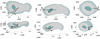 |
Fig. 1 Cut-views of the 3D numerical model with the exterior shape corresponding to that of the asteroid 25143 Itokawa (Fujiwara et al. 2006). The signal paths between the transmitter (Tx) and the receiver (Rx) are also shown in various cut-views through the model. The real part of the exact relative permittivity distribution for the DM is piecewise constant with the values εr = 1, εr = 2.56 + j0.02, and εr = 3.4 + j0.04 inside the ellipsoidal internal void, in the mantle layer, and elsewhere within the asteroid body, respectively. |
Signal parameters used in simulating the electric field propagation.
5 Results
5.1 Electric field inside the analogue
Figure 2 depicts a simulated electric field E propagation inside the DM analogue at two frequencies 2 and 10 GHz. This total field differs significantly from the incident field and the influence of multiple scattering is clearly visible at 10 GHz, while it is present already at 2 GHz. This is due to the size of the target and its contrast, and suggests the inadequacy of linear propagation (single scattering, i.e., scattering under Born approximation) models as they omit the effects of multiple scattering or multiple coupling including multiple reflections and refractions, which are also referred to as multi-path effects determined by the second term on the right-hand side of Eq. (3). At 2 GHz, the main dimension of the analogue is equal to 2.5 λm with λm denoting the wavelength in the medium. The amplitude of the field is almost constant within the analogue and that is why the outline of the mantle and the void can be clearly distinguished. At 10 GHz, the target is larger in terms of the wavelength, that is, the main dimension of the analogue is equal to 12.6 λm, and the field inside includes fine ripples which correspond to multiple paths and scattering effects due to the high contrast between the permittivity of the analogue and that of the vacuum.
5.2 Time–frequency analysis
Figure 3 includes the time–frequency analysis of the scattered field corresponding to DM and HM. The temporal zones corresponding to travel-times scattering from the different parts of the analogues are distinguished (Table 2) according to Eyraud et al. (2020), that is, Mantle I (the first mantle reflection), Void (scattering by the void), Mantle II (the reflection on the opposite side of the asteroid with respect to the first one), Higher-order (multiple scattering), and second-order reflection zones. The travel times can be seen as annotations for linking the time axis to the space and they provide guidance as to which peaks in the data correspond to which space in the object. These are based on our previous careful analysis (Eyraud et al. 2020) and are includedhere to help the reader to understand the time–space correspondence. The scattering signatures of the two analogues are relatively similar. The major signatures are in the frequency band 2.6–9.1 GHz. A weaker signal is visible also in the frequency 11.1–12.4 GHz. For the other frequencies, the signature is comparably weak, ≤ − 20 dB with respectto the maximal amplitude of the scattered signal.
Figure 3 also compares the cases of 32 and 8 frequency bands of width ≈ 0.4 and ≈ 1.6 GHz, respectively, of which the latter allows a better temporal resolution. Based on the results, it is obvious that while the ≈ 0.4 GHz bandwidth essentially corresponds to a single scattered wavefront (between 12 and 13.7 ns) caused by the asteroid body as a whole, the greater bandwidth ≈1.6 GHz enables us to distinguish between the wavefronts originating from the Mantle I and Mantle II zones, that is, from the two opposite sides of the analogue model, and can therefore be considered as a minimal bandwidth for detecting interior details in the time domain.
Notably, the scattered signal corresponding to the DM has a greater intensity not only in the direct scattering zone but also in the higher-order zone (between 2 and 9 GHz) as compared to the HM analogue, which is visible in the difference between the two signatures. In summary, this analysis shows not only that it is possible to detect the interior structures of asteroids by considering direct reflections, but also that these structures can be deduced by analysing the higher-order zone when the temporal resolution is sufficient to separate this zone from the others which seems the case at ≥ 1.6 GHz bandwidth.
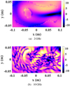 |
Fig. 2 Magnitude (in dB) of the calculated field inside the DM analogue. |
5.3 Bornapproximation
The spatial distribution of the BA was analysed for the time points t1 –t5 described inTable 2. The spatial plots are shown in Fig. 4 for the demodulated BA (Eq. (15)) with three different regularisation parameter values, ν = 2E-2 (optimised via bracketing), ν = 2E-4 (underregularised), and ν = 2 (overregularised), and for the amplitude-based BA (Eq. (16)) with just the first of these, ν = 2E-2. In relation to the maximum absolute value of the denominator in Eq. (13), these values are 1E-3, 1E-5, and 1E-1, respectively.
In Fig. 5, the first and second rows from the top show the full demodulated wave and its amplitude for the locations p1 –p5, respectively. The third to sixth rows illustrate the complete normalised BA at p1 –p5, revealing the effect of the parameter choice on the regularised deconvolution process (Takala et al. 2018; Sorsa et al. 2020). Overall, the most regular outcome can be observed to result with the value ν = 2E-2 (third row). Oscillation artifacts were found to occur when the regularisation parameter is either larger or smaller than this value; their frequency increases when the parameter is decreased. In the case of overregularisation ν = 2 (fourth row), the deconvoluted signal has pre-ringing artifacts. That is, the fluctuations start before the actual pulse response occurs. The underregularised outcome obtained with ν = 2E-4 (fifth row) is corrupted by high-frequency noise. The sixth row of Fig. 5 shows the optimal regularisation parameter for the amplitude-based BA.
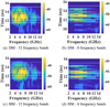 |
Fig. 3 Time–frequency analysis for the two analogues with a variation of the frequency bands. The horizontal lines correspond to the temporal zones indicated by Table 2. |
Scattering zones and time points t1−t5 for evaluating the BA.
5.4 Backpropagation
5.4.1 In time domain
From the scattered field obtained in a quasi-monostatic configuration at a single point, structural imaging maps were obtained by backpropagation using two algorithms, one in the time domain and the other in the frequency domain. The time domain fields corresponding to the simulation and measurement are visualised in Fig. 6. Backpropagation was carried out first from calculations and then from experimental data measured in the anechoic chamber of the Centre Commun de Ressources en Microondes (CCRM) in Marseille Eyraud et al. (2020).
Figure 7 shows the backpropagated reconstructions obtained via the demodulation and amplitude-based BA and visualised for an increasing amount of simulated time-domain data. By visual comparison to the exact DM structure, which is shown in the background of each reconstruction, the superior outcome is obtained, when Mantle I to Mantle II, and Mantle I to Higher order scattering zones are included in the data. These reconstructions, shown framed in the middle of the figure, account for the best localisation of the void area and suggest that the mantle is also detectable in Mantle I zone, that is, on the side corresponding to the signal transmission and measurement.
The laboratory measurement data of Eyraud et al. (2020) obtained with the 3D-printed DM was applied to calculate backprojection reconstructions shown in Fig. 8. Also, in this case, the superior reconstructions are obtained when the zones from Mantle I to Mantle II and up to the Higher order scattering zone are included in the data (centre frame). Although generally similar in comparison to the simulated data in Fig. 7, the measured data yield more focused reconstruction around the void area especially in the cut-view along the z-axis.
Common to the reconstructions shown in Figs. 7 and 8 is a slight deviation of the observed void location away from the receiver which might be due to the absence of the mantle in HM which is applied as the point of linearisation for the BA. Moreover, comparison between the results obtained with the demodulation and amplitude-based BA shows that the reconstruction of the void appears more distinct in the former case, while the mantle appears more pronounced in the latter.
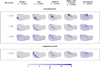 |
Fig. 4 Effect of the deconvolution regularisation parameter on the volume-normalised BA of the QAM signal “Demodulated BA”, d in Eq. (15), and the BA of the amplitude-based signal “Amplitude-based BA”, |

5.4.2 In frequency domain
The maps reconstructed with backpropagation using the simulated and measured field data are plotted in Figs. 9 and 10, respectively. These maps correspond to the sum of the gradients for the different frequencies at the first iteration according to Eq. (19). For the results from calculations the frequency band 2–10 GHz is used and for the results from measurements, the frequency band 4–18 GHz is used. In the measurements, the low frequencies (2–4 GHz) are eliminated because these measuring points are more noisy because the antenna pattern is not very directional at these frequencies.
In these figures, the positions of the different boundaries (air/mantle, mantle/interior, interior/void, void/interior, interior/mantle, mantle/air) are plotted with different colours. For interfaces air/mantle, mantle/interior, interior/mantle, and mantle/air, the coloured area correspond to the calculated position with ± 15% accuracy considering that Born approximation is used (including a distance compensation). The void area is the size of the void in the direction orthogonal to the wave propagation with Born distance compensation. The corresponding values are given in Table 3.
Firstly, it can be noted that the reconstructed areas are, as expected, orthogonal to the direction of wave propagation. Looking to the maps reconstructed from the calculations (Fig. 9), the two boundaries between the air and the target are visible for both DM and HM objects. For the DM analogue, an additional signature is reconstructed inside the target which corresponds to the void. We note that the two air/object and object/air interfaces are in the correct areas for both analogues and that the interface inside the object (for the DM analogue) is appropriately within the void area. The mantle/interior and interior/mantle interfaces (for DM analogue) are not visible.
Considering the maps reconstructed from the measurements (Fig. 10), it is still possible to see the two air/target and target/air boundaries for the HM analogue. We note that the target/air boundary is somewhat shifted. For the DM analogue, the air/target boundary is visible (but slightly shifted), and the target/air boundary is missing. The void signature (shifted) is also visible in the reconstruction.
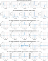 |
Fig. 5 Full temporal wave analysed for the five different locations p1–p5 as indicated by circled dots in the top row of Fig. 4. These locations correspond to the spatial maximiser of the BA for the time points t1 –t5, respectively. The vertical lines show the zone interfaces in Table 2 with the red lines outlining the higher order zone. The two top rows show the BA and its amplitude at the fixed point along the time domain as it propagates through the object. The four bottom rows show the BA at these time points. The row ordering follows that of Fig. 4 and clearly illustrates the effect of the Tikhonov regularisation parameter ν on the deconvolution. The data in each plot have been normalised spatially with respect to the transmitter distance. |
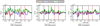 |
Fig. 6 Time domain data obtained via QAM. Two left columns: demodulated in-phase (solid red), quadrature component (dashed blue), and amplitude (solid light green) obtained for the DM analogue via simulation and measurement, respectively.Right column: simulated data obtained for HM analogue. The vertical lines illustrate the temporal zones of Table 2. The red vertical lines indicate the higher order scattering zone. |
6 Discussion
Here we analyse full microwave propagation and backpropagation with a structurally complex asteroid analogue model as a target. This analogue was first 3D printed as a plastic wire-frame structure applying the recently introduced permittivity control method of Saleh et al. (2021) after which quasi-monostatic laboratory experiments were performed (Eyraud et al. 2020). The thorough analysis performed for a single measurement point, which is the worst-case scenario for a space radar, constitutes an important feasibility study for observing the interior structure of the analogue based on the experimental measurement data of Eyraud et al. (2020).
Our results obtained in both the frequency and time domains show that the internal void and mantle compartments of the analogue can be reconstructed by backpropagating the full wave field. We find that the properties of the BA applied in the backpropagation process affect the reconstruction quality. In particular, the temporal coverage of the data used in computing the BA is found to have a significant effect on the performance. The most detailed description of the interior structure of the asteroid is obtained when Mantle I, Void, Mantle II, and Higher-order scattering zone are covered by the data, and excluding the second-order reflection zone is found to be necessary. An optimised regularisation parameter was applied in calculating the BA to ensure that the results are of the best quality possible.
Our results demonstrate the feasibility of revealing the details of the interior an asteroid analogue with a realistic shape and complex structure via full wave-field modelling. Our findings support the previous observation that a peak signal-to-noise ratio (S/N) of 10 dB between the measured and simulated wave field might be sufficient for observing the interior structures, as suggested by Sorsa et al. (2019) who rely on numerical simulations in their study. In the present measurement dataset, this limit is achieved for the Mantle I, Void, and Mantle II zones described by Eyraud et al. (2020). Moreover, parallel to the previous findings of Sorsa et al. (2020); Eyraud et al. (2020), we find higher order scattering effects to be significant with respect to the quality of the BA and therefore the reconstruction.
While the present implementation of BA in the time domain takes into account both direct and indirect (higher order) scattering effects, its accuracy decreases as time elapses. Modelling the second-order reflections corresponding to long (double side-to-side) signal propagation paths was found to lead to a noisy outcome and to corrupt the backpropagated reconstructions, and therefore we found it necessary to limit the temporal range of the data. The present frequency domain approach to backpropagation shows that the interior structures can be distinguished based on the full data set without any information about the surface shape or mean permittivity inside the asteroid. In this case, the wavefield considered in BA is that of vacuum.
The backpropagation approaches of this study are relatively simple and may therefore be expected to lead to slight mispositioning of the interior structures: firstly, in the frequency domain, no permittivity approximation for the interior part of the asteroid model is made (so it is vacuum), and in the time domain, the permittivity estimate relies on an a priori measurement performed for a test sphere (Eyraud et al. 2020), but is not optimised using the dataset obtained for the analogue. Secondly, the first-order BA is applied on the direct and adjoint problem, meaning that the multiple scattering or coupling effects are omitted. Thus, it is immediately clear that the reconstruction quality might be improved by applying more advanced backpropagation techniques which we regard as a challenging future work topic. For instance, the higher order BA developed in Sorsa et al. (2020) or the wave-field tomography proposed in Sava & Asphaug (2018b), both in the time domain, as well as full-wave inversion developed in the frequency domain (Eyraud et al. 2012, 2019), constitute potential approaches to take into account the high-order scattering effects. Namely, the slightly biased void location in the reconstructions obtained in this study might be corrected if the non-linear signal interaction effects between the void and mantle compartments inside the analogue are taken into account which is the case in the higher order BA or full-wave inversion. Another approach is to consider a transformed or complementary data modality, such as for instance the travel-time, which has been applied in CONSERT (Kofman et al. 2007, 2015), for example. The differences revealed by the present modalities, that is, the demodulated signal and its amplitude, support this assumption. Advanced travel-time inversion schemes have been developed, especially for seismic inversion (Luo et al. 2016; Tarantola & Santosa 1984; Tarantola 2005), in which the data are likely to be scarce –akin to space missions–, but also for electromagnetic investigation of a small Solar System body (Sava & Asphaug 2018a).
As we show that the interior structure of an asteroid analogue can be observed with a minimal number of full-wave measurements, despite its complex realistic shape, the relevance of the present results is significant with respect to future missions, such as for example Hera (Michel et al. 2018), as well as to the many proposed missions and mission concepts involving the use of radar data to probe the largely unknown interior structure of the small Solar System bodies (Asphaug et al. 2002, 2008; Barucci et al. 2005; Bambach et al. 2018; Snodgrass et al. 2018). With respect to mission design, the important aspects in this study are the frequency range and bandwidth of the signals modelled. The analogue scale applied here is partially limited by the equipment laboratory radar experiment. We consider the most relevant scales with respect to mission design to be those corresponding to 10 (Binzel & Kofman 2005) and 20 MHz (Kofman 2012) centre frequencies.
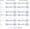 |
Fig. 7 Tomographic backprojection (adjoint operation of BA) obtained with the simulated data with the signal path shown in Fig. 1. Reconstructions are shown in blue for both the demodulated BA (left) and the amplitude-based BA (right) and for the temporal ranges of data as specified by zones in Table 2. The exact DM model structure with the surface layer and the void is shown in the reconstruction background. |
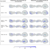 |
Fig. 8 Tomographic backprojection (adjoint operation of BA) done with microwave radar measurement data. Reconstructions are shown in blue for both the demodulated BA (left) and the amplitude-based BA (right) and for the temporal ranges of data as specified by zones in Table 2. The exact DM model structure with the surface layer and the void is overlaid in the reconstruction background. |
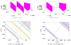 |
Fig. 9 Reconstructions obtained by backpropagation in the frequency domain using the calculated fields with a single transmitter and a single receiver and the frequency band between 2 and 10 GHz. The direction of wave propagation is plotted with a dashed line. The coloured areas corresponding to the different parts of the analogue, taking into account the Born compensation and their boundaries, are summarised in Table 3: the green one refers to the boundaries air/mantle and mantle/air, the blue one refers to the reflections mantle/interior and interior/mantle, and the yellow one refers to the reflections interior/void and void/interior. |
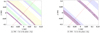 |
Fig. 10 Reconstructions obtained by backpropagation in the frequency domain using the measured fields with a single transmitter and a single receiver and the frequency band between 4 and 18 GHz. The direction of wave propagation of the wave is plotted as a dashed line. The coloured areas are as in Fig. 9. |
7 Conclusion
We demonstrate the feasibility of reconstructing the details inside a structurally complex asteroid analogue model with a realistic shape and internal permittivity structure based on the current knowledge of asteroid interiors from sparse measurements, such as those from quasi-monostatic full microwave data measured at a single point. The results and the applied signal configuration and parameters are significant in the design of future space missions aiming to reconstruct the interior structure of small Solar System bodies. The quality of the backpropagation results obtained depend on the applied modelling strategy, signal modality, data coverage, and inversion procedure, the latter motivating future inversion method development.
Important goals for the future include a full tomographic imaging experiment including wider coverage of measurements; for example, multi-monostatic or bistatic. Analogue development towards more arbitrary permittivity structures will be examined to further strengthen the mission-relevance of the results. Advanced reconstruction strategies will also be investigated, including for example theeffect of data modality, taking into account the non-linearity of the inversion procedure, and the introduction of a priori information on the target.
Acknowledgement
The authors acknowledge Jean-Michel Geffrin, who performed the measurements and provided the data, and the opportunity provided by the Centre Commun de Ressources en Microondes (CCRM) to use its fully equipped anechoic chamber. We acknowledge the Mesocentre of Aix Marseille University for its support for these calculations. L.-I.S. was supported by a Young Researcher’s Grant from Emil Aaltonen Foundation. L.-I.S., and S.P. were supported by the Centre of Excellence in Inverse Modelling and Imaging (Academy of Finland 2018-2025, project number 312341) and the Academy of Finland project number 336151. L.-I.S. and S.P. acknowledge CSC – IT Center for Science Ltd., for providing computing services on the Puhti supercomputer.
References
- Asphaug, E., Ryan, E. V., & Zuber, M. T. 2002, Asteroids III (Tucson: University of Arizona Press), 1, 463 [Google Scholar]
- Asphaug, E., Scheeres, D., & Safaeinili, A. 2008, 37th COSPAR Scientific Assembly, held 13-20 July 2008, in Montréal, Canada, 37, 139 [Google Scholar]
- Bambach, P., Deller, J., Vilenius, E., et al. 2018, Adv. Space Res., 62, 3357 [CrossRef] [Google Scholar]
- Barrowes, B. E., Teixeira, L. F., & Kong, J. A. 2001, Microw. Opt. Technol. Lett., 31, 28 [CrossRef] [Google Scholar]
- Barucci, M. A., D’Arrigo, P., Ball, P., et al. 2005, High. Astron., 13, 738 [CrossRef] [Google Scholar]
- Bertero, M., & Boccacci, P. 1998, Opt. Photonics News 12, 46 [Google Scholar]
- Binzel, R. P., & Kofman, W. 2005, C. R. Phys., 6, 321 [CrossRef] [Google Scholar]
- Blair, D. M., Chappaz, L., Sood, R., et al. 2017, Icarus, 282, 47 [CrossRef] [Google Scholar]
- Carry, B. 2012, Planet. Space Sci., 73, 98 [NASA ADS] [CrossRef] [Google Scholar]
- Eyraud, C., Litman, A., Hérique, A., & Kofman, W. 2009, Inverse Prob., 25, 024005 [CrossRef] [Google Scholar]
- Eyraud, C., Geffrin, J.-M., Litman, A., & Spinelli, J.-P. 2012, Rad. Sci., 47, 1 [CrossRef] [Google Scholar]
- Eyraud, C., Saleh, H., & Geffrin, J.-M. 2019, J. Opt. Soc. Am. A, 36, 234 [CrossRef] [Google Scholar]
- Eyraud, C., Sorsa, L.-I., Geffrin, J.-M., et al. 2020, A& A, 643, A68 [CrossRef] [Google Scholar]
- Fujiwara, A., Kawaguchi, J., Yeomans, D., et al. 2006, Science, 312, 1330 [NASA ADS] [CrossRef] [PubMed] [Google Scholar]
- Grima, C., Kofman, W., Mouginot, J., et al. 2009, Geophys. Res. Lett., 36, 101 [Google Scholar]
- Harrington, R. 1987, J. Electromagn. Waves Appl., 1, 181 [CrossRef] [Google Scholar]
- Haruyama, J., Kaku, T., Shinoda, R., et al. 2017, Lunar Planet. Sci. Conf., 48, 1711 [Google Scholar]
- Hayabusa Project Science Data Archive 2007, Itokawa shape model, https://darts.isas.jaxa.jp/planet/project/hayabusa/shape.pl, accessed 4 November, 2019 [Google Scholar]
- Herique, A., Gilchrist, J., Kofman, W., & Klinger, J. 2002, Planet. Space Sci., 50, 857 [CrossRef] [Google Scholar]
- Hérique, A., Agnus, B., Asphaug, E., et al. 2018, Adv. Space Res., 62, 2141 [CrossRef] [Google Scholar]
- Hérique, A., Plettemeier, D., Kofman, W., et al. 2019, in EPSC Abstracts, 13, EPSC-DPS Joint Meeting 2019, Geneva, Switzerland [Google Scholar]
- Jutzi, M., & Benz, W. 2017, A&A, 597, A62 [NASA ADS] [CrossRef] [EDP Sciences] [Google Scholar]
- Kaku, T., Haruyama, J., Miyake, W., et al. 2017, Geophys. Res. Lett., 44, 10 [CrossRef] [Google Scholar]
- Kofman, W. 2012, Radar Wireless Commun., 2, 409 [Google Scholar]
- Kofman, W., Herique, A., Goutail, J.-P., et al. 2007, Space Sci. Rev., 128, 413 [NASA ADS] [CrossRef] [Google Scholar]
- Kofman, W., Herique, A., Barbin, Y., et al. 2015, Science, 349, aab0639 [Google Scholar]
- Luo, Y., Ma, Y., Wu, Y., Liu, H., & Cao, L. 2016, Geophysics, 81, R261 [CrossRef] [Google Scholar]
- Merchiers, O., Eyraud, C., Geffrin, J.-M., et al. 2010, Opt. Exp., 18, 2056 [CrossRef] [Google Scholar]
- Michel, P., Kueppers, M., Sierks, H., et al. 2018, Adv. Space Res., 62, 2261 [NASA ADS] [CrossRef] [Google Scholar]
- Picardi, G., Plaut, J. J., Biccari, D., et al. 2005, Science, 310, 1925 [CrossRef] [Google Scholar]
- Saleh, H., Tortel, H., Leroux, C., et al. 2021, IEEE Trans. Ant. and Prop., in press [Google Scholar]
- Sava, P., & Asphaug, E. 2018a, Adv. Space Res., 62, 1146 [CrossRef] [Google Scholar]
- Sava, P., & Asphaug, E. 2018b, Adv. Space Res., 61, 2198 [CrossRef] [Google Scholar]
- Snodgrass, C., Jones, G., Böhnhardt, H., et al. 2018, Adv. Space Res., 62, 1947 [CrossRef] [Google Scholar]
- Sorsa, L.-I., Takala, M., Bambach, P., et al. 2019, ApJ, 872, 44 [CrossRef] [Google Scholar]
- Sorsa, L., Takala, M., Eyraud, C., & Pursiainen, S. 2020, IEEE Trans. Comput. Imaging, 6, 579 [CrossRef] [Google Scholar]
- Takala, M., Bambach, P., Deller, J., et al. 2018, IEEE Trans. Aerospace Electronic Syst. [Google Scholar]
- Tarantola, A. 2005, Inverse Problem Theory and Methods for Model Parameter Estimation (Philadelphia: SIAM) [Google Scholar]
- Tarantola, A., & Santosa, F. 1984, Inverse Problems of Acoustic and Elastic Waves (Philadelphia: SIAM), 104 [Google Scholar]
- van der Vorst, H. A. 2003, Iterative Krylov Methods for Large Linear Systems (Cambridge: Cambridge University Press), 95 [CrossRef] [Google Scholar]
- Vernazza, P., Jorda, L., Ševeček, P., et al. 2020, Nat. Astron., 4, 136 [CrossRef] [Google Scholar]
All Tables
All Figures
|
Fig. 1 Cut-views of the 3D numerical model with the exterior shape corresponding to that of the asteroid 25143 Itokawa (Fujiwara et al. 2006). The signal paths between the transmitter (Tx) and the receiver (Rx) are also shown in various cut-views through the model. The real part of the exact relative permittivity distribution for the DM is piecewise constant with the values εr = 1, εr = 2.56 + j0.02, and εr = 3.4 + j0.04 inside the ellipsoidal internal void, in the mantle layer, and elsewhere within the asteroid body, respectively. |
| In the text | |
|
Fig. 2 Magnitude (in dB) of the calculated field inside the DM analogue. |
| In the text | |
|
Fig. 3 Time–frequency analysis for the two analogues with a variation of the frequency bands. The horizontal lines correspond to the temporal zones indicated by Table 2. |
| In the text | |
|
Fig. 4 Effect of the deconvolution regularisation parameter on the volume-normalised BA of the QAM signal “Demodulated BA”, d in Eq. (15), and the BA of the amplitude-based signal “Amplitude-based BA”, |
| In the text | |
|
Fig. 5 Full temporal wave analysed for the five different locations p1–p5 as indicated by circled dots in the top row of Fig. 4. These locations correspond to the spatial maximiser of the BA for the time points t1 –t5, respectively. The vertical lines show the zone interfaces in Table 2 with the red lines outlining the higher order zone. The two top rows show the BA and its amplitude at the fixed point along the time domain as it propagates through the object. The four bottom rows show the BA at these time points. The row ordering follows that of Fig. 4 and clearly illustrates the effect of the Tikhonov regularisation parameter ν on the deconvolution. The data in each plot have been normalised spatially with respect to the transmitter distance. |
| In the text | |
|
Fig. 6 Time domain data obtained via QAM. Two left columns: demodulated in-phase (solid red), quadrature component (dashed blue), and amplitude (solid light green) obtained for the DM analogue via simulation and measurement, respectively.Right column: simulated data obtained for HM analogue. The vertical lines illustrate the temporal zones of Table 2. The red vertical lines indicate the higher order scattering zone. |
| In the text | |
|
Fig. 7 Tomographic backprojection (adjoint operation of BA) obtained with the simulated data with the signal path shown in Fig. 1. Reconstructions are shown in blue for both the demodulated BA (left) and the amplitude-based BA (right) and for the temporal ranges of data as specified by zones in Table 2. The exact DM model structure with the surface layer and the void is shown in the reconstruction background. |
| In the text | |
|
Fig. 8 Tomographic backprojection (adjoint operation of BA) done with microwave radar measurement data. Reconstructions are shown in blue for both the demodulated BA (left) and the amplitude-based BA (right) and for the temporal ranges of data as specified by zones in Table 2. The exact DM model structure with the surface layer and the void is overlaid in the reconstruction background. |
| In the text | |
|
Fig. 9 Reconstructions obtained by backpropagation in the frequency domain using the calculated fields with a single transmitter and a single receiver and the frequency band between 2 and 10 GHz. The direction of wave propagation is plotted with a dashed line. The coloured areas corresponding to the different parts of the analogue, taking into account the Born compensation and their boundaries, are summarised in Table 3: the green one refers to the boundaries air/mantle and mantle/air, the blue one refers to the reflections mantle/interior and interior/mantle, and the yellow one refers to the reflections interior/void and void/interior. |
| In the text | |
|
Fig. 10 Reconstructions obtained by backpropagation in the frequency domain using the measured fields with a single transmitter and a single receiver and the frequency band between 4 and 18 GHz. The direction of wave propagation of the wave is plotted as a dashed line. The coloured areas are as in Fig. 9. |
| In the text | |
Current usage metrics show cumulative count of Article Views (full-text article views including HTML views, PDF and ePub downloads, according to the available data) and Abstracts Views on Vision4Press platform.
Data correspond to usage on the plateform after 2015. The current usage metrics is available 48-96 hours after online publication and is updated daily on week days.
Initial download of the metrics may take a while.