| Issue |
A&A
Volume 643, November 2020
|
|
|---|---|---|
| Article Number | A100 | |
| Number of page(s) | 29 | |
| Section | Cosmology (including clusters of galaxies) | |
| DOI | https://doi.org/10.1051/0004-6361/201936592 | |
| Published online | 10 November 2020 | |
One- and two-point source statistics from the LOFAR Two-metre Sky Survey first data release
1
Fakultät für Physik, Universität Bielefeld, Postfach 100131, 33501 Bielefeld, Germany
e-mail: t.siewert@physik.uni-bielefeld.de
2
Astrophysics, University of Oxford, Denys Wilkinson Building, Keble Road, Oxford OX1 3RH, UK
3
CSIRO Astronomy and Space Science, PO Box 1130, Bentley, WA 6102, Australia
4
Institute of Cosmology & Gravitation, University of Portsmouth, Dennis Sciama Building, Burnaby Road, Portsmouth PO1 3FX, UK
5
Department of Physics & Astronomy, University of the Western Cape, Private Bag X17, Bellville, Cape Town 7535, South Africa
6
Leiden Observatory, Leiden University, PO Box 9513, 2300 Leiden, RA, The Netherlands
7
ASTRON, the Netherlands Institute for Radio Astronomy, Postbus 2, 7990 Dwingeloo, AA, The Netherlands
8
SUPA, Institute for Astronomy, Royal Observatory, Blackford Hill, Edinburgh EH9 3HJ, UK
9
Centre for Astrophysics Research, School of Physics, Astronomy and Mathematics, University of Hertfordshire, College Lane, Hatfield AL10 9AB, UK
10
GEPI & USN, Observatoire de Paris, Université PSL, CNRS, 5 Place Jules Janssen, 92190 Meudon, France
11
Department of Physics & Electronics, Rhodes University, PO Box 94, Grahamstown 6140, South Africa
12
RAL Space, The Rutherford Appleton Laboratory, Chilton, Didcot OX11 0NL, UK
13
Department of Physical Sciences, The Open University, Walton Hall, Milton Keynes MK7 6AA, UK
Received:
28
August
2019
Accepted:
28
August
2020
Context. The LOFAR Two-metre Sky Survey (LoTSS) will eventually map the complete Northern sky and provide an excellent opportunity to study the distribution and evolution of the large-scale structure of the Universe.
Aims. We test the quality of LoTSS observations through a statistical comparison of the LoTSS first data release (DR1) catalogues to expectations from the established cosmological model of a statistically isotropic and homogeneous Universe.
Methods. We study the point-source completeness and define several quality cuts, in order to determine the count-in-cell statistics and differential source count statistics, and measure the angular two-point correlation function. We use the photometric redshift estimates, which are available for about half of the LoTSS-DR1 radio sources, to compare the clustering throughout the history of the Universe.
Results. For the masked LoTSS-DR1 value-added source catalogue, we find a point-source completeness of 99% above flux densities of 0.8 mJy. The counts-in-cell statistic reveals that the distribution of radio sources cannot be described by a spatial Poisson process. Instead, a good fit is provided by a compound Poisson distribution. The differential source counts are in good agreement with previous findings in deep fields at low radio frequencies and with simulated catalogues from the SKA Design Study and the Tiered Radio Extragalactic Continuum Simulation. Restricting the value added source catalogue to low-noise regions and applying a flux density threshold of 2 mJy provides our most reliable estimate of the angular two-point correlation. Based on the distribution of photometric redshifts and the Planck 2018 best-fit cosmological model, the theoretically predicted angular two-point correlation between 0.1 deg and 6 deg agrees reasonably well with the measured clustering for the sub-sample of radio sources with redshift information.
Conclusions. The deviation from a Poissonian distribution might be a consequence of the multi-component nature of a large number of resolved radio sources and/or of uncertainties on the flux density calibration. The angular two-point correlation function is < 10−2 at angular scales > 1 deg and up to the largest scales probed. At a 2 mJy flux density threshold and at a pivot angle of 1 deg, we find a clustering amplitude of A = (5.1 ± 0.6) × 10−3 with a slope parameter of γ = 0.74 ± 0.16. For smaller flux density thresholds, systematic issues are identified, which are most likely related to the flux density calibration of the individual pointings. We conclude that we find agreement with the expectation of large-scale statistical isotropy of the radio sky at the per cent level. The angular two-point correlation agrees well with the expectation of the cosmological standard model.
Key words: large-scale structure of Universe / galaxies: statistics / cosmology: observations / radio continuum: galaxies
© ESO 2020
1. Introduction
The LOFAR Two-metre Sky Survey (LoTSS; Shimwell et al. 2017)1, carried out with the LOw Frequency ARray (LOFAR; van Haarlem et al. 2013), will provide the deepest and best resolved inventory of the radio sky at low frequencies over the coming decades. Having already produced high fidelity images and catalogues over 424 square degrees at a central frequency of 144 MHz (Shimwell et al. 2019), LoTSS will continue to produce a catalogue that is estimated to contain about 15 million radio sources over all of the Northern hemisphere. A large fraction of those sources will come with optical identifications (Williams et al. 2019) and photometric redshifts (Duncan et al. 2019). For the first data release, already about half of the radio sources have measured photometric redshifts. In addition to this, the WEAVE-LOFAR survey (Smith et al. 2016), using the William Herschel Telescope Enhanced Area Velocity Explorer (WEAVE; Dalton et al. 2012, 2014), will measure spectroscopic redshifts for about a million sources from the LoTSS catalogue. The survey is, therefore, not only expected to provide a rich resource for astrophysics, but also for cosmology, see, for example, Raccanelli et al. (2012), Camera et al. (2012), Jarvis et al. (2015), and Maartens et al. (2015). Together with photometric redshifts and, at a later stage, spectroscopic redshifts, we will be able to measure the luminosity and number density evolution directly; additionally, through a clustering analysis, we will also be able to measure the relative bias between the different radio source populations.
Extragalactic radio sources are tracers of the large-scale structure of the Universe. The evolution of the large-scale structure in turn depends on many fundamental parameters; for example, it depends on the model of gravity, the proportion of visible and dark matter as well as dark energy, and the primordial curvature fluctuations. Unfortunately, these dependencies are blended with unknowns from astrophysics, such as the bias factors for active galactic nuclei (AGN) and starforming galaxies (SFG), their number density, and luminosity evolutions. The purpose of this work is to take a first step towards the cosmological analysis of LoTSS.
For cosmological studies, surveys must cover a sizeable fraction of the sky and sample the sky fairly homogeneously, down to some minimal flux density. Currently available radio surveys in the LoTSS frequency range are the TIFR GMRT Sky Survey (TGSS-ADR1; Intema et al. 2017) and the GaLactic and Extragalactic All-sky MWA survey (GLEAM; Hurley-Walker et al. 2017). The first alternative data release of the TGSS covers 36 900 square degrees of the sky at a central frequency of 147.5 MHz and at an angular resolution of 25″. A seven-sigma detection limit with a median root mean square (rms) noise of 3.5 mJy beam−1 results in 623 604 sources. Comparing the measured TGSS source counts to SKADS (SKA Design Study, Wilman et al. 2008) sky simulations shows good agreement for flux density thresholds above 100 mJy. The GLEAM catalogue covers 24 831 square degres and contains 307 455 sources with 20 separate flux density measurements between 72 MHz and 231 MHz, centred at 200 MHz at an angular resolution of 2′. The catalogue is estimated to be 90% complete at a flux density threshold of 170 mJy in the entire survey area for a five-sigma detection limit. The rms noise varies between 10 mJy beam−1 and 23 mJy beam−1 along four declination ranges, which complicates the measurements of cosmic structures on large angular scales.
As LoTSS will eventually cover all of the Northern sky and detect about 15 million radio sources, it will allow us to overcome statistical limitations due to shot noise and substantially reduce cosmic variance in cosmological analyses, two issues in which contemporary wide area radio continuum catalogues suffer.
In this work we study the one- and two-point statistics for the sources in the LoTSS data release 1 (DR1). Covering an area of 424 square degress over the Hobby-Eberly Telescope Dark Energy Experiment (HETDEX; Hill et al. 2008) spring field, DR1 contains 325 694 radio sources, detected by means of PYBDSF (Python Blob Detector and Source Finder2, Mohan & Rafferty 2015) with a peak flux density of at least five times the local rms noise. The median rms noise in the observed area is 71 μJy beam−1 at an angular resolution of 6″. The LoTSS-DR1 value-added catalogue, as described by Williams et al. (2019) removes artefacts and corrects wrong groupings of Gaussian components. It contains 318 520 sources of which 231 716 have optical and/or near-IR identifications in surveys of the Panoramic Survey Telescope and Rapid Response System (Pan-STARRS; Kaiser et al. 2002, 2010) and the Wide-field Infrared Survey Explorer (WISE; Wright et al. 2010).
Before the LoTSS catalogues can be used for cosmological analyses, the consistency of the flux density and the completeness and reliability of the detected sources must be carefully examined. For cosmological analyses, we are interested in the large scale features on the sky, and large scale instrumental or calibration effects must be identified and accounted for, before we can draw credible cosmological conclusions.
The goal of this work is therefore to recover and re-establish the well known and tested properties of large-scale structure in the radio sky. The study of the one- and two-point number count statistics of the LoTSS-DR1 value-added catalogue offers an excellent opportunity to do so, and the cleaning and quality control methods presented in this work will provide a good basis for future cosmological exploitation of LoTSS.
The potential of radio continuum surveys for cosmology has been studied in detail in the context of the SKA, see, for example, Jarvis et al. (2015), Square Kilometre Array Cosmology Science Working Group (2020) and its precursors, among them LOFAR (Raccanelli et al. 2012). Some of the cosmological SKA science cases can already be tackled by LoTSS, even well before regular SKA surveys will start. In the pre-SKA era, a key topic of investigation will be to improve our understanding of dark energy and modified gravity; these can be parametrised so that we can constrain, for example, the equation of state of dark energy and its evolution, the deviation of the relationship between density and potential from that expected in the Poisson equation, and the ratio of the space- and time-parts of the metric. These parameters have observable consequences via their effect on the expansion history and/or structure growth history of the Universe. This in turn affects the predictions for observable cosmological probes, including the auto-correlation of source counts, the cross-correlation of source counts with the Cosmic Microwave Background (CMB; integrated Sachs-Wolfe effect, Ballardini & Maartens 2019), and the cross-correlation of source counts at different redshifts (which is activated by gravitational lensing magnification effects). The radio sky also provides an opportunity to constrain primordial non-Gaussianity in the distribution of density modes in the Universe (Ferramacho et al. 2014; Raccanelli et al. 2015); this is observable as an enhanced autocorrelation at large angular scales. In addition, very wide surveys can probe the kinematic and matter radio dipole (Bengaly et al. 2019), which can act as a fundamental test of the cosmological principle. Here we focus on the simplest statistical tests, in particular the two-point source count statistics.
In Sect. 2 we summarise the theoretical expectation for the one- and two-point number counts. In Sect. 3 we describe how we identify the survey regions that are most reliable, estimate the completeness of LoTSS-DR1 and describe the masks and flux density cuts that we apply to the data. In order to compare expectation and data, we generate mock catalogues, which are described in Sect. 4. The properties of the one-point statistics are discussed in Sect. 5. For this, we ask if the radio sources in a pixel on the sky are drawn from a Poisson process and we investigate the differential number counts and then compare them to other surveys and to simulations. In Sect. 6 we estimate the two-point statistics, the angular correlation function, which we fitted to a phenomenological model and compare them to findings from previous surveys, as well as to the theoretically expected angular two-point correlation function based on the Planck 2018 best-fit cosmological model, the photometric redshift distribution found for LoTSS-DR1 radio sources, and a bias function from the literature. We present our conclusions in Sect. 7.
This work is complemented by four Appendices. In Appendix A we describe a masking procedure for the TGSS-ADR1 catalogue that is used for comparison and estimate the corresponding angular two-point correlation function. Five common estimators for the angular two-point correlation function are described and compared in the context of LoTSS-DR1 in Appendix B. We also test the accuracy of the software package TREECORR (Jarvis et al. 2004) that we use for the computation of the angular two-point correlation function by means of an independent, computationally slow but presumably exact brute force algorithm (Appendix C). In Appendix D we show that the contribution of the kinematic radio dipole to the angular two-point correlation function is negligible for the angular scales probed in this work.
2. Large scale structure in radio continuum surveys
Before we investigate the data, we first discuss what the standard model of cosmology predicts for the statistical tests that we will consider throughout this work.
2.1. Source counts in cells
The cosmological principle is fundamental to modern cosmology, stating that on large enough scales the distribution of matter and light is isotropic and homogeneous on spatial sections of space-time. Isotropy on large scales is observed at a wide range of frequencies, from the distribution of radio sources, to the distribution of gamma-ray bursts, and is most precisely tested by means of the cosmic microwave sky (see e.g. Peebles 1993; Planck Collaboration XVI 2016; Planck Collaboration VII 2020). Therefore we also expect to find an statistically isotropic distribution of extragalactic radio sources for LoTSS, which means that the expectation value of the number of radio sources per unit solid angle, or surface density σ, with flux density above a certain threshold Smin, is independent of the position on the sky e. The number counts in a pixel (or cell) of solid angle Ωpix centred at e are

with (ensemble) expectation value

The simplest model for the distribution of radio sources assumes that they are (i) identically and (ii) independently distributed, and (iii) pointlike (i.e. it is possible to reduce the pixel size until each pixel would contain at most one fully contained source). These assumptions define what is called a homogenous Poisson process (see e.g. Peebles 1980). Thus the naive expectation is that the probability of finding k sources above a flux density threshold Smin in any cell of fixed size is given by a Poisson distribution with intensity parameter λ:

with expectation ![$ \bar{N} \equiv \mathrm{E}[k] = \lambda $](/articles/aa/full_html/2020/11/aa36592-19/aa36592-19-eq4.gif) and variance
and variance ![$ \mathrm{Var}[k] = \lambda = \bar{N} $](/articles/aa/full_html/2020/11/aa36592-19/aa36592-19-eq5.gif) .
.
Deviations from a Poisson distribution are expected due to effects from gravitational clustering of large-scale structure [a violation of condition (ii)], resolved sources [a violation of condition (iii)], and multi-component sources, such as FRII radio galaxies in which the radio lobes are not statistically independent from each other [violation of condition (ii)]. Different types of radio sources could follow different statistical distributions, which would then violate condition (i). These effects and additional observational systematics are expected in radio continuum surveys, and thus we must expect that radio sources should not be perfectly Poisson distributed.
Let us consider the expected modifications due to multiple radio components and show that this effect can be modelled by means of a compound Poisson distribution (James 2006), meaning that the distribution that follows from adding up n identically distributed and mutually independent random counts ni, with i = 1 to n, and n itself follows a Poisson distribution with mean β. Let us first assume that the number of radio components is also Poisson distributed. Then the probability p to find k sources in a cell follows from  , where the first factor is the conditional probability to find k radio components, like distinct hot spots and the core, associated with n galaxies and the second factor is the probability to have n galaxies. We further assume γ is the mean number of components per galaxy and thus the mean of the conditional probability is nγ. This results in
![$$ \begin{aligned} p_k ^{\mathrm{CP} }= \sum _{n=0}^{ \infty }\left[\frac{(n\gamma )^k e^{-n\gamma }}{k!} \frac{\beta ^n e^{-\beta }}{n!}\right], \end{aligned} $$](/articles/aa/full_html/2020/11/aa36592-19/aa36592-19-eq7.gif)
with expectation and variance now given by
![$$ \begin{aligned} \bar{N} \equiv \mathrm{E} [k]=\beta \gamma , \qquad \mathrm{Var} [k]=\beta \gamma (1+\gamma ) = \bar{N} (1+\gamma ). \end{aligned} $$](/articles/aa/full_html/2020/11/aa36592-19/aa36592-19-eq8.gif)
Thus, we see that unidentified multiple radio components can increase the variance of the source counts, for example, for a textbook FRII with a detected core we would see three components which would immediately lead to an increase of the variance. This statement is independent of the size of the cell, but how many radio components can be identified does depend on the angular resolution and completeness of the radio continuum survey.
It is useful to define the clustering parameter (Peebles 1980)
![$$ \begin{aligned} n_\mathrm{c} \equiv \frac{\mathrm{Var} [k]}{\mathrm{E} [k]}, \end{aligned} $$](/articles/aa/full_html/2020/11/aa36592-19/aa36592-19-eq9.gif)
which is a proxy for the number of sources per “cluster”. For the Poisson distribution nc = 1, while nc = 1 + γ for a compound Poisson distribution. Groups of radio sources, like a group of SFGs, also contribute to nc, and thus nc is also a tracer of clustering at small angular scales. The measurement of nc alone can not distinguish between galaxy groups, multi-component sources, and imaging artefacts.
Whilst we believe assuming a Poisson distribution for the number of radio components per physical source will be appropriate for this work, we can chose another distribution, which will result in another compound distribution. To give a second example, assuming a logarithmic distribution results in a negative binomial distribution (James 2006), which interestingly provides the best-fit to three dimensional counts-in-cell in the Sloan digital sky survey (Hurtado-Gil et al. 2017).
2.2. Differential source counts
While counts in cells provides information on the spatial distribution of radio sources, it is also interesting to study their distribution in flux density. The number of sources per solid angle and per flux density observed at radio frequency ν, or the so-called differential source count is given by
where σ is the source density and we assume that the specific luminosity can be written as a power-law, Lν ∝ ν−α, with spectral index α, and ϕ(Lν, α; z) is the comoving luminosity density of radio sources at redshift z. In reality radio sources show a distribution in α, often assumed to be a fixed value 0.7–0.8. A LOFAR study of radio sources in the Lockman hole compared to NVSS sources measured a median spectral index α = 0.78 ± 0.015 (Mahony et al. 2016), with errors obtained by bootstrapping. In a study of spectral indices comparing NRAO VLA Sky Survey (NVSS, Condon et al. 1998) and TGSS-ADR1 sources an averaged  (de Gasperin et al. 2018) was found, which is comparable to measurements by Hurley-Walker et al. (2017) with median and semi-inter-quartile-range α = 0.78 ± 0.20 for flux densities S < 0.16 Jy at 200 MHz in the GLEAM survey. This also matches the finding by Tiwari (2019), who estimated a mean spectral index of
  for sources with flux densities STGSS ≥ 100 mJy and SNVSS ≥ 20 mJy. For the sake of simplicity, we assume here that all radio sources have the same spectral index. The relationship between spectral luminosity and flux density is given by:
In Eq. (9) we express the surface density by the luminosity density and integrate it over the past light-cone. This introduces the dependence on the Hubble rate at particular redshift H(z) and an extra factor involving the transverse comoving distance (or proper motion distance)
where H0 denotes today’s Hubble rate and Ωk denotes the dimensionless curvature parameter, which is positive, zero, or negative for hyperbolic, flat, or spherical space, respectively. If we were to live in a static Universe with Euclidean geometry, the differential source counts would be proportional to S−5/2 (Condon et al. 1988). Observations of source counts are typically rescaled by this factor to highlight the evolution of the Universe and of radio sources.
2.3. Angular two-point correlation function
In order to study the clustering of radio sources and to use them as a probe of the large-scale structure of the Universe, the third quantity of interest in this work is the angular two-point correlation function.
We denote the angular two-point correlation function of radio sources above a given flux density threshold S = Smin by w(e1, e2, S), which is in principle a function of four position angles and the flux density threshold. It measures how likely it is to find k1 sources within a solid angle Ω at position e1 and at the same time find k2 sources around e2 within Ω in excess of what would be found for a isotropic distribution of sources:
The cosmological principle tells us that the correlation function should be isotropic, which means that it is invariant under rigid rotations of the sky, and thus should only depend on the angle θ = arccos(e1 ⋅ e2), such that:

As a square integrable function on the interval cos θ ∈ [ − 1, 1] can be expressed as a series of Legendre polynomials Pℓ(cos θ), this can allow w to be rewritten as:
The coefficients Cℓ are called the angular power spectrum.
In this work, we will parametrise the two-point correlation function by a simple power-law:
which is the result of several approximations (Totsuji & Kihara 1969; Peebles 1980), including Limber’s equation (Limber 1953) relating the angular correlation function to its spatial counterpart. The amount of correlation A* is defined at the pivot angular scale θ*, which we fix at 1 deg. We arrive at the form in Eq. (15) based on the following assumptions: the power spectrum of matter density fluctuations the P(k, z) is assumed to be scale free; the bias, b(k, z) (Mo & White 1996),(Sheth & Tormen 1999; Wilman et al. 2008; Raccanelli et al. 2012; Tiwari & Nusser 2016), is assumed to preserve the scale-free spectrum; lensing and other relativistic effects are ignored and we consider only small angular separations, meaning θ ≪ 1 rad.
While we use the power-law parametrisation (15) in order to compare to the two-point correlation function found in other studies of radio surveys (Kooiman et al. 1995; Rengelink et al. 1999; Blake & Wall 2002; Overzier et al. 2003; Blake et al. 2004; Rana & Bagla 2019; Dolfi et al. 2019), we would like to note that this approximation is not accurate enough to enable the extraction of interesting information on cosmological parameters. Studies of the NVSS catalogue measured typical values of A ∼ 10−3 and γ ∼ 1 (Blake & Wall 2002; Overzier et al. 2003; Blake et al. 2004), while first studies of TGSS-ADR1 data revealed much larger amplitudes A ∼ 10−2 and comparable values of γ (Rana & Bagla 2019; Dolfi et al. 2019).
In order to compare the angular two-point correlation function to the prediction from the standard model of cosmology and going beyond the approximations that lead to Eq. (15), we use the publicly available software package CAMB SOURCES3 (Challinor & Lewis 2011); more details are provided in Sect. 6.
The two-point correlation function and angular power spectrum for source counts is of great value in informing us about cosmology. We can fit parametrised theoretical models to the data, hence finding the range of acceptable parameters. One cannot constrain cosmological parameters individually, but rather a combination of parameters which all affect the observable. With upcoming data releases of LoTSS, we plan to investigate the following parameters relevant to cosmology:
(i) The bias parameters (Mo & White 1996; Sheth & Tormen 1999; Tiwari & Nusser 2016; Hale et al. 2018) reveal the relationship between source count fluctuations and underlying total density fluctuations, as a function of scale and time. These can give insight into the astrophysics-cosmology interface, informing us about the range of halo masses that radio sources inhabit. Further to this, with Halo Occupation Distribution Modelling (HOD; see descriptions and uses in e.g. Berlind & Weinberg 2002; Zheng et al. 2005; Hatfield et al. 2016), the properties of how galaxies occupy dark matter haloes can be determined. This will be especially important with deep radio observations, such as the LOFAR deeper tier surveys (Rottgering 2010; van Haarlem et al. 2013), where it may be possible to observe the “1-halo” clustering (see e.g. Yang et al. 2003; Zehavi et al. 2004), which describes the clustering between radio sources in the same parent dark matter halo. By observing both the “2-halo” and “1-halo” term and modelling the observed clustering within a HOD framework, it is possible to determine quantities which describe the distribution of central and satellite galaxies for different radio source populations. Finally, if the cross correlation function is instead investigated, the clustering observed may also be important in investigating how different radio sources within single dark matter haloes may be affected by other galaxies within the same halo (see e.g. Hatfield & Jarvis 2017).
(ii) Parameters describing the total density of matter, Ωm, and the rms amplitude of fluctuations in the matter density in a sphere of 8 h−1 Mpc, σ8, will affect P(k, z). We note that Ωm tells us about the degree to which dark matter dominates the matter budget in the Universe, whilst σ8 relates to the degree to which structures have grown by the present day.
(iii) Dark energy parameters, like the equation of state of dark energy at scale factor a, which is given by w = w0 + (1 − a)wa (Chevallier & Polarski 2001; Linder 2003), where the present day equation of state is w0, and its time evolution is parametrised by wa, affect the growth of structure and hence enter into P(k, z).
(iv) The growth of structure is also affected by parameters describing modifications to gravity (Amendola et al. 2008; Zhao et al. 2010), like the slip parameter η, which is the ratio of the space- and time- perturbations in the metric. In addition we can examine the Poisson equation ∇2Φ = 4πGa2μρδ, where μ parametrises deviations from the GR expectation μ = 1.
(v) Finally, primordial non-Gaussianity of density modes affects the measured two-point statistics (Dalal et al. 2008; Matarrese & Verde 2008; Ferramacho et al. 2014; Raccanelli et al. 2015). On large scales, the effective bias is greatly increased, leading to a substantial increase in amplitude of the auto-correlation function or power spectrum. Constraints on the non-Gaussianity parameter fNL are expected to improve on constraints by Planck.
3. LoTSS-DR1: data quality
3.1. Requirements and cell size
To study the cosmic large scale structure, we require three essential properties of a radio survey. First of all, the survey must cover a sizeable fraction of the sky in order to measure properties on large angular scales and to ensure that the effects of interest are not dominated by cosmic variance. Secondly, the survey must sample the sky fairly homogeneously to some minimal flux density, which then allows for reliable and complete source counts. Thirdly, in order to identify foreground effects and to classify radio sources, identification with an optical or infra-red counterpart and associated photometric or spectroscopic redshift, is essential.
In order to connect number counts with theoretical predictions, we must estimate σ(S, e) by counting radio sources in cells of equal and non-overlapping areas, a necessary (but not sufficient) condition for the statistical independence of the counts. Finally, these cells should cover the sky completely. Thus, we need to select a scheme to pixelize the sky and for this pixelisation we need to decide how large those cells should be. The pixel sizes of the LoTSS imaging pipeline and used by the source finder PYBDSF are too small to be efficient for cosmological tests (most of them contain only noise) and it would be computationally expensive to correlate all pixel pairs. On the other hand, the individual LoTSS pointings are too large to define cell sizes that are useful for cosmological analysis, as there are about 6000 sources per pointing.
The scheme in HEALPIX4 (Górski et al. 2005) is one such method that satisfies the above requirements (equal area, no overlap, complete sky coverage) and has been developed for the purpose of the analysis of the cosmic microwave background. We use it in the so-called ring scheme, which numbers the cells in rings of decreasing declination. In order to avoid confusion with imaging pixels, we will denote HEALPIX pixels as cells in the following. The cell size is specified by means of the parameter Nside, which can take values of 2m, where m is an integer. The total number of cells on the sky is given by  .
.
For each cell, we count the number of radio sources, either in the catalogue originally produced by PYBDSF (LoTSS-DR1 radio source catalogue) or in the final LoTSS-DR1 value-added source catalogue, where radio components of a single source have been grouped and artefacts removed. The position of each source was taken as either the output position from PYBDSF or the RA and Dec value that was assigned in the value-added catalogue (see Williams et al. 2019 for a description of how these were generated).
The mean number of sources per cell is
where Nsurvey and Ωsurvey denote the total number of sources and the total solid angle covered by the survey. We want to find a value of Nside, that guarantees that all cells contain at least one source, if the cell was properly sampled, meaning that each cell area should be completely within the survey area and we would like to disregard regions with very low completeness. We assume that the source counts are Poisson distributed and estimate the probability that a cell does not contain a source as

The probability that all cells contain at least one source is then given by P = (1 − p0)Ncell, with  is the number of cells covering the survey area. We wish to keep the probability to find empty cells, P0(Nside) = 1 − P ≈ p0Ncell well below one, but at the same time would like to allow for the best angular resolution. With Ωsurvey = 424 square degrees (0.12916 sr) and Nrs = 325 694 we find P0(256) = 3 × 10⁻¹⁴, while P0(512) is of order unity. In a resolution of Nside = 256, the cells have a mean spacing of
  deg and a cell covers Ωpix ≈ 1.60 × 10⁻⁵ sr. The set of all non-empty cells defines the effective survey area. The number of cells within the survey area for the chosen Nside and after masking can be seen in Table 1. Figure 1 shows the cell counts of the LoTSS-DR1 radio source catalogue at a resolution of Nside = 256, which is a good compromise between large enough cell size to make sure that the shot noise in each cell is not the dominant feature (i.e. all cells contain at least one source) and to retain as much angular resolution as possible. One can also see that plotting the number counts per cell has advantages over a map that shows each radio source as a dot, as such a map quickly saturates when the surface density of objects is high (see Fig. 1).
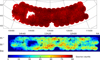 |
Fig. 1. Distribution of radio sources observed in the LoTSS-DR1 HETDEX spring field. Plotted are all individual sources (top), as well as the number counts per cell in Cartesian projection at HEALPIX resolution Nside = 256 (bottom). Observed are nearly 325 000 sources within 58 pointings on the sky covering 424 square degrees. The positions of the five brightest radio sources in terms of integrated flux density are indicated in black (see Sect. 3.3 for details). |
Number of included cells (Ncell) and sky coverage (Ω) for different masks and flux density thresholds (Smin).
3.2. Completeness
The LoTSS-DR1 catalogue was generated by combining 58 individual LOFAR pointings on the sky. The current LOFAR calibration and imaging pipeline used in DR1 produces sub-standard images in a few places due to poor ionospheric conditions and/or due to the presence of bright sources. Such areas are not included. Furthermore, in some regions, where the astrometric position offsets from Pan-STARRS is large, the LoTSS maps are blanked. This results in an inhomogeneous sampling of the HETDEX spring field as is apparent from the source density map presented in Fig. 1.
We estimated the point source completeness of all pointings in the HETDEX field by injecting random sources in the residual maps and using the same PYBDSF set up used for the LoTSS-DR1 radio source catalogue. Only sources with flux densities five times greater than the local rms noise are retained. The completeness itself is estimated by taking the fraction of recovered sources to the total number of injected sources above a certain flux density threshold. In total we simulated 50 samples with 6000 sources each for each of the 58 pointings. The completeness of each pointing is shown in Fig. 2, where pointings at the edge of the survey are marked in green and pointings in the inner field are marked in blue. Additionally, five pointings are marked in red, which are clearly undersampled, for reference see Table 2. Using all pointings, the survey is 95% point source complete at 0.43 mJy and reaches 99% completeness at 1.0 mJy. Rejecting the five most incomplete pointings, the 95% level is at 0.39 mJy and the 99% level is reduced to 0.80 mJy.
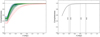 |
Fig. 2. Left: estimated point-source completeness for each of the 58 pointings in the HETDEX field as a function of flux density. Blue, green and red (dotted) lines indicate inner, outer and the five most incomplete pointings, respectively. Right: mean point source completeness of all pointings (solid line) and after rejection of the five most incomplete pointings (dotted line). |
Undersampled pointings with name and position.
As we use HEALPIX cells to determine the source count statistics, we estimate the completeness for each cell. Without any flux density threshold the completeness per cell is shown in Fig. 3. The structure of the completeness across the survey matches the number density of Fig. 1. Areas with high number densities appear to be already more complete without assuming any flux density threshold and underdense regions are comparable to areas with low completeness. Applying a flux density threshold of 0.39 mJy, corresponding to a point source completeness of 95% in the region without the five pointings of Table 2, results in a much improved uniformity of the completeness (see also Fig. 3).
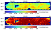 |
Fig. 3. Top: completeness of the LoTSS-DR1 catalogue per HEALPIX cell. Bottom: completeness of cells after applying a flux density threshold of 0.39 mJy, which corresponds to an overall point source completeness of 95%. |
3.3. Consistency of source counts
Completeness and total source counts will be a function of the distance from the pointing centre, as the sensitivity is not uniform across the primary beam. This is investigated by means of radial source counts around the pointing centres. All sources within angular distance, θ, from the pointing centre are counted and the sum is normalised by the solid angle of the corresponding disc. We split the pointings into three groups, depending on their position and whether they appear undersampled (see Table 2). In Fig. 4 we show source counts for pointings at the edge of the HETDEX field (green), inner pointings (blue) and pointings which are excluded from the further analysis (red dotted). The mean source counts of all pointings is shown in black, with the 1σ region in grey. The source counts of green pointings drop after the angular distance reaches regions which are not covered by overlapping pointings of the survey any more. Pointings in the inner field have more continuous source counts, as they overlap with other pointings. The five undersampled pointings from the latter appear in this test also as the undersampled ones.
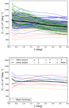 |
Fig. 4. Top: source counts for each pointing within angular distance θ around the pointing centre, normalised by covered area. Pointings are classified by position in the HETDEX field, with pointings on the edge (green), in the inner field (blue) and undersampled ones (red, dotted). The mean is shown in black with standard deviation (grey band) of all pointings. Bottom: source counts around the five brightest radio sources in terms of integrated flux density from the radio source (dashed lines) and value-added source catalogue (solid lines). The mean number counts around the five brightest sources are shown in black for both catalogues and additionally also the mean over all pointings (dash dotted). |
Additionally, we study the source counts around the five brightest sources. The five sources are listed in Table 3 and are the same in the LoTSS-DR1 radio source and value-added catalogues. They are displayed in Fig. 1 as black circles to show the underlying regions. Comparing both catalogues, the radio source catalogue shows a stronger effect on the source counts due to limited dynamic range around bright sources. This effect is visible by eye in Fig. 1 (bottom), where the bright sources are located in underdense regions. In contrast, in the value-added catalogue the mean of sources becomes flatter, because many sources are matched together. Overall we see a deficit of sources around the five brightest sources compared to the overall mean of all pointings, but that deficit is well within the variance of source counts and thus we decided to keep regions that include bright sources in our analysis.
Five brightest sources of LoTSS-DR1 in terms of total flux density.
3.4. Survey area
A proper definition of the survey area directly affects the one- and two-point statistics, especially the mean surface density. As we exclude all sources of the five most incomplete pointings (see Table 2), it is therefore important to define the region being investigated throughout this work, excluding these pointings.
To remove the sources of those five pointings and to model the boundaries of the survey, we produce a mask (mask p). We model each pointing as a disc with radius of 1.7 deg, inferred from the (average) radius of pointings in the mosaic and mask all cells which are not included in the union of all discs (see Fig. 5). We verified that this procedure does not result in a single empty cell, consistent with the argument that we used to set the value of Nside.
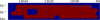 |
Fig. 5. LoTSS-DR1 HETDEX spring field masks: “mask p” rejects all cells shown in dark blue and includes 53 pointings modelled by discs of radius 1.7 deg. Our default “mask d” additionally rejects cells with less than five sources (yellow cells), see also text in Sect. 3.4. For analysis that includes redshift information “mask z” additionally rejects a strip shown in light blue. For further details, see the text in Sect. 5.3. |
We test for the robustness of this method by also masking cells containing fewer than five sources. This results in removing another six cells and 14 sources. We adopt this slightly stronger mask (mask d) as the basis of our analysis. The total number of sources and the effective survey area for the various masks and cuts can be found in Table 1. Our base mask (mask d) applied to the LoTSS-DR1 catalogue results in a mean number of sources per cell of  and a mean surface density of
  = 798.6 deg−2 = 0.2218 arcmin−2.
The histogram for the masking that excludes the five bad pointings and all cells with less than five sources is shown in Fig. 6. For comparison we also plot a Poisson distribution with identical mean. We observe a broadening of the source count distribution when compared to a Poisson distribution, which obviously is not a good fit to the data. Thus we see that the naive expectation about the number count distribution is not met.
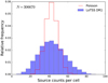 |
Fig. 6. Histogram of source counts per cell (blue) and binned Poisson distribution with empirical mean (red line) from the LoTSS-DR1 radio source catalogue at Nside = 256, masked and including only cells with at least five sources (mask d). |
3.5. Local rms noise
To further characterise the properties of LoTSS-DR1, we take a closer look at the properties of the local rms noise. We define a set of tiered masks to reject cells with noise above certain noise thresholds.
Fluctuations in the local rms noise are expected for several reasons. In the vicinity of bright sources, limitations of dynamic range give rise to an increase of the local rms noise. Directions and epochs with unfavourable ionospheric conditions will also result in higher noise levels. To find regions of higher noise, we therefore produced a HEALPIX map of the local rms per HEALPIX cell, as well as the corresponding histogram of the local rms noise distribution (see Fig. 7). The map is produced by averaging the local rms noise associated to each source in the cell, which is defined as the averaged background rms value of the corresponding island, obtained from the LoTSS-DR1 catalogue.
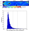 |
Fig. 7. Local rms noise per HEALPIX cell, calculated via the mean of the local rms around each LoTSS-DR1 radio source. The heat map (top) and histogram (bottom) of the local rms is clipped at an upper limit of five times the median rms noise. The median rms noise of 0.07 mJy beam−1, as well as the values of two and three times the median rms noise are marked in the histogram with black dashed lines. |
Using the local rms noise attached to each source gives rise to a slightly larger cell average, than doing cell averages on the noise maps themselves. This effect is due to bright sources, which increase the noise. The mean local rms noise of the HEALPIX cells is 94 μJy beam−1 and median local rms noise in a cell is 76 μJy beam−1, which is in good agreement with the median rms noise 71 μJy beam−1 in the total observed area based on the much smaller mosaic pixels (Shimwell et al. 2019).
To produce a tiered set of noise masks, we require the local rms noise to be below one, two, and three times the median rms noise of 0.07 mJy beam−1 and denote the resulting masks by mask 1, mask 2, and mask 3, respectively. Most of the sources are unaffected with the 0.21 mJy beam−1 and 0.14 mJy beam−1 rms mask, but for the upper limit of 0.07 mJy beam−1 rms noise (mask 1), we obtained less than 50 percent of the original number of sources (see Table 1). The difference in the masking can also be seen in the remaining number of cells Ncell and sky coverage Ω (see Table 1). These noise masks are shown in Fig. 8.
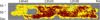 |
Fig. 8. Sky coverage of the three local rms noise masks. The red cells are included for an average noise < 0.07 mJy beam−1 in the HEALPIX cells (“mask 1”), red and yellow pixels are included for an average noise of < 0.14 mJy beam−1 (“mask 2”) and red, yellow and light blue cells are included for an average noise of < 0.21 mJy beam−1 (“mask 3”). Dark blue cells are additionally included in “mask d”. Regions in grey are excluded by all masks. |
We also checked that the variance of the number count distribution becomes smaller with decreasing the upper rms noise limit. We return to more details of the statistical evaluation in Sect. 5.
In the analysis below, we combine spatial masking with flux density thresholds in order to improve the completeness and reliability of the studied sample of radio sources. The faintest, at five times signal to local noise, observed radio sources in the LoTSS-DR1 survey have a flux density of around 0.1 mJy, and, as shown above, the survey is certainly not complete at such low flux densities. Thus, below we test different flux density thresholds to increase the completeness and reliability of the survey. The source counts corresponding to flux density thresholds (for unresolved sources) of five, ten, and 15 times the rms noise of the masked survey are listed in Table 1 for both the LoTSS-DR1 radio source and the value-added source catalogue. We can easily see that a cosmological data analysis has to find a good compromise between high demands on data quality (more aggressive masking and higher flux density thresholds) and the demand for statistics (large number of radio sources).
4. Mock catalogues
As discussed in Sect. 2.3, the two-point correlation function quantifies the excess in clustering observed within a galaxy catalogue at different separation scales compared to that of a uniform distribution of galaxies. As such, it is necessary to construct a mock random catalogue which is a realistic distribution of sources that could be observed but has no knowledge of large scale structure. With a uniform noise distribution, this would involve constructing a catalogue where random positions across the observable survey area are selected. However, as can be seen in Fig. 7, the noise across the field of view is non-uniform. This will affect how sources of different flux densities can be detected across the field of view. To account for this non-uniform noise, therefore, and its effect on the detection of sources when constructing a random catalogue, we follow the method of Hale et al. (2018).
To obtain a mock catalogue that accurately reflects radio sources that could be observed with LOFAR, we make use of the SKA Design Study Simulated Skies (SKADS; Wilman et al. 2008, 2010). These extragalactic simulated catalogues provide a realistic distribution of sources that could be observed across 100 square degrees, with flux density measurements at five frequencies ranging from 151 MHz to 18 GHz. These sources are a mixture of both AGN as well as SFGs and have further information on the type of AGN Fanaroff & Riley (1974) Type I/II sources as well as radio quiet quasars) or SFG (i.e. normal star forming galaxy or starburst). As these SKADS catalogues have realistic radio flux density distributions, they are used to construct a mock catalogue by comparing whether the flux density of a randomly generated source from the SKADS catalogue could be observed above the noise within the LoTSS image.
Therefore, the rms maps from LoTSS were used to determine whether a randomly generated source would be detectable above the noise and could realistically be observed. To generate a mock catalogue, random positions within the observed region were generated and a flux density from the SKADS catalogue were also assigned to the sources. Under the assumption that the source is unresolved, the flux density from SKADS5 was combined with a randomly generated flux density to account for the noise at the position (see Hale et al. 2018) to form a total ‘measured’ flux density. This noise was selected from a normal distribution centred on zero with a sigma given by the rms at that position. The measured flux density for a source was then compared to the rms noise at the location of the source. A source only remained within the mock catalogue if this measured flux density was at least five times greater than the rms value at its position. We generated enough random positions until we had roughly a total of 20 times the number of detected sources of the LoTSS- DR1 radio source catalogue.
The distribution of the sources within this mock catalogue (after masking has been applied) can be seen in Fig. 9.
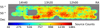 |
Fig. 9. Mock catalogue of random sources that are detectable at five times the local rms noise and masked with “mask d”. |
5. One-point statistics
5.1. Distribution of radio source counts
As shown in Sect. 3, the distribution of number counts is broader than expected for a Poisson distribution. The naive assumption of a Poisson distribution arises from the expectation of a homogeneous and isotropic universe and independent, identically distributed and point-like radio sources.
There are at least four contributions to a deviation from a homogeneous spatial Poisson process: (a) multi-component sources (Magliocchetti et al. 1998), (b) fluctuations of the calibration, (c) confused sources (several sources are counted as a single source), (d) cosmic structure. Here we investigate the statistical properties of the counts in cell by measuring moments of the empirical counts-in-cell distribution and comparing it to theoretical models.
Let ki denote the counts in the ith cell. Then the central moments of a sample map are given by:
with the sample mean:
To analyse the counts-in-cell statistics, we calculate the clustering parameter nc (see Eq. (6)) as a function of the flux density threshold. We also calculate the coefficients of skewness (g1) and excess kurtosis (g2 − 3) (Zwillinger & Kokoska 2000):
For the Poisson distribution, Eq. (3), with λ = μ, we find:
and  .
.
For the compound Poisson distribution (Eq. (4)),

and nc = 1 + γ. With βγ = μ we can rewrite the coefficients as:
![$$ \begin{aligned}&g_1^\mathrm{CP} = \frac{1}{\root \of {\mu }}\left[\frac{n_\mathrm{c} ^2+n_\mathrm{c} -1}{n_\mathrm{c} ^{3/2}}\right], \end{aligned} $$](/articles/aa/full_html/2020/11/aa36592-19/aa36592-19-eq34.gif)
![$$ \begin{aligned}&g_2^\mathrm{CP} -3= \frac{1}{\mu }\left[\frac{n_\mathrm{c} ^3+3n_\mathrm{c} ^2-2n_\mathrm{c} -1}{n_\mathrm{c} ^{2}}\right]. \end{aligned} $$](/articles/aa/full_html/2020/11/aa36592-19/aa36592-19-eq35.gif)
In Fig. 10 we show the clustering parameter nc (red circles) and the coefficients of skewness (blue triangle) and excess kurtosis (yellow squares) for the LoTSS-DR1 radio source and the LoTSS-DR1 value-added source catalogues as a function of flux density threshold and for three different masks (mask d, mask 2 and mask 1). Error bars are computed from 100 bootstrap samples, but are in most cases smaller than the symbol. It can be seen that for the lowest flux density thresholds nc is well above unity, but at flux density thresholds above 1 mJy, the clustering parameter is almost constant and only slightly above unity. It approaches unity faster for the value added catalogue. It is also interesting to observe that the radio source catalogue shows a strong evolution of excess kurtosis g2 − 3 with increasing flux density threshold, except for noise mask 1, which masks all but the cleanest cells. In contrast, the value-added catalogue shows the qualitatively expected behaviour for excess kurtosis and skewness for all masks considered. The value-added catalogue differs from the original radio source catalogue in a statistically significant way, especially with respect to higher moments, despite the fact that the number of sources in both catalogues differs by less than 2 per cent.
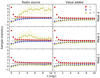 |
Fig. 10. Sample statistics of number counts in cells as a function of flux density threshold. Shown are the clustering parameter nc (variance over mean), which is expected to be one for the Poisson distribution, the skewness g1 and excess kurtosis g2 − 3 with error bars calculated from 100 bootstrap samples. On the left hand side for the LoTSS-DR1 radio source catalogue, on the right hand side for the LoTSS-DR1 value-added source catalogue. From top to bottom: mask d and masks 2 and 1. |
In Fig. 11 we compare the observed coefficients of skewness and excess kurtosis of the LoTSS-DR1 value-added source catalogue with “mask d” to their theoretical expected values for a Poisson and a compound Poisson distribution. We observe that the compound Poisson distribution provides a significant improvement over the Poisson distribution, which extends to values well into the regime in which we can regard the catalogue to be complete.
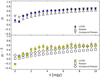 |
Fig. 11. Skewness (g1) and excess kurtosis (g2 − 3) of the masked LoTSS DR1 value-added source catalogue (mask d), also plotted are the expected moments of a Poisson and compound Poisson distribution. Errors bars for the data sample are computed from bootstrap sampling. |
To further quantify the quality of the fit, we tested both distributions with a Pearson chi-square test for four different flux density thresholds applied on the LoTSS-DR1 value-added catalogue with mask d. The results of that test are shown in Fig. 12 and Table 4. While the coefficient of skewness shows very nice agreement between the compound Poisson distribution and the data, the coefficient of excess kurtosis shows better agreement with the compound Poisson distribution compared with the Poisson distribution. In terms of the Pearson χ2-test the compound Poisson distribution describes the data significantly better than the Poisson distribution, see Table 4. Values of χ2/d.o.f. of order unity indicate a good fit. For the 1 mJy sample, this ratio is 30.7 and 0.76 for the Poisson and compound Poisson distributions, respectively.
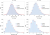 |
Fig. 12. Histograms of LoTSS-DR1 counts-in-cell for the flux density thresholds 1, 2, 4 and 8 mJy. Also shown are the best-fit Poisson and compound Poisson distributions. |
Pearson χ2-test statistic of counts-in-cell distribution for the masked LoTSS-DR1 value-added source catalogue with “mask d” for four flux density thresholds.
We conclude that the counts-in-cell distribution of the LoTSS-DR1 value-added catalogue is not Poissonian. The compound Poisson distribution provides an excellent fit to the data, but other distributions (not studied in this work) might also provide a good fit to the data.
We can also test if the mock catalogue shows the same statistical behaviour as the data. Their clustering parameter and coefficients of skewness and excess kurtosis are shown in Fig. 13. In order to compare the mock catalogue to the LoTSS-DR1, we randomly draw sub-samples of the mock catalogue that contain the same number of data points as the LoTSS-DR1 value-added source catalogue. At S > 1 mJy, we find that the clustering parameter in the mocks is closer to one and the higher statistical moments are closer to a Poisson distribution than the LoTSS-DR1 value-added source catalogue. We checked that fitting a compound Poisson distribution to the mocks also improves the fits (as there are more free parameters), but not by as much in the case of the LoTSS-DR1 value added source catalogue. We thus conclude that there are indeed clustering effects in the LoTSS-DR1 data on top of the effects that are taken care of in the mock catalogue.
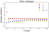 |
Fig. 13. Clustering parameter and coefficients of skewness and kurtosis for a sub-sample of the mock catalogue, which matches the size of the value-added source catalogue. Error bars are computed from bootstrap sampling. |
5.2. Differential source counts
Let us now turn our attention to the differential source counts as a function of flux density (we use the integrated flux density for all sources). In Fig. 14 we plot the differential number counts of the LoTSS-DR1 value-added source catalogue with Euclidean normalisation, meaning that in a static, homogeneous and spatially flat Universe the normalised counts would be constant as a function of flux density. The bins in the differential number counts plot have equal step width in log10(S). We determine the source counts for four masks (masks d, 1, 2, and 3) applied.
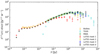 |
Fig. 14. Differential number counts per flux density interval of the masked LoTSS-DR1 value-added source catalogue for four different masks. Additionally the masked TGSS-ADR1 (147.5 MHz; this work, blue circle), the LOFAR Boötes field (Williams et al. 2016, orange triangle) and the MWA (154 MHz; Franzen et al. 2016, green box) are shown. Error bars for the LoTSS and TGSS counts are due to Poisson noise in each flux density bin, which have equal step width in log10(S). |
The errors are assumed to follow Poisson noise in each bin. This assumption seems to be in contradiction to our findings from the previous section. Therefore, we alternatively estimated the errors by means of 100 bootstrap samples of the masked survey. Sample mean and standard deviation of the 100 bootstrap samples turn out to be in agreement with analysis that just assumes Poisson noise for each bin. Surprisingly, the bootstrap sample variance tends to be slightly smaller over the complete flux density range. For simplicity and to be on the safe side we thus show the Poisson noise only. Stating the fact that the value-added and masked source catalogue is 95% point-source complete at 0.39 mJy (note that this is for the total source counts, the differential counts at that flux density are already incomplete), we refrain from applying any completeness corrections to the differential number counts, but instead work with flux density thresholds.
Figure 14 shows that noise “mask 1”, and to lesser extent “mask 2”, result in a lack of sources at high flux densities. This can be easily understood as masking regions with larger rms noise selects regions that include the high-flux density sources, since limited dynamic range leads to increased rms noise in their neighbourhood. At low flux densities, applying the strongest noise mask (mask 1), the differential number counts show increased completeness at low flux densities compared to all other masks. This difference shows up below 1 mJy. This is an independent confirmation that the value-added source catalogue has a high degree of completeness at S > 1 mJy. This test also allows us to argue that it is not only point source complete, but also shows a high degree of completeness for extended sources, as this test does not distinguish between point sources and resolved sources. Independently from the arguments given in the previous section, we arrive at the conclusion that we can trust the source counts at S > 1 mJy.
For comparison we also plot the masked source counts for the TGSS-ADR1 radio source catalogue, which agree very well with the LoTSS-DR1 value-added source counts for flux densities between 80 mJy and 20 Jy. In order to obtain the differential number counts of the TGSS-ADR1, we masked the Milky Way with a cut in galactic latitude at |b| ≤ 10 deg, discarded unobserved regions and missing pointings with a HEALPIX mask at Nside = 32. On top we applied a noise mask with an upper cut in local rms noise of 5 mJy beam−1 (see Appendix A and Fig. A.1). For the TGSS there are more sources detected at higher flux densities than shown in the differential source counts as we focus on the available flux density range defined by the LoTSS-DR1 sample. The decreasing trend of the source counts at higher flux densities is not physical and can be explained by the masking procedure. Masking with larger cells at the same noise levels will average over larger regions and therefore samples over larger number of sources. Therefore bright and noisy sources will be more often taken into account in the analysis than by masking with higher resolutions.
Additionally, we also plot the differential source counts from Franzen et al. (2016) obtained with the MWA 154 MHz survey and from Williams et al. (2016) obtained with LOFAR at 150 MHz from the Boötes field. We find that the LoTSS-DR1 value-added source catalogue agrees well with these existing studies. We note that no completeness corrections (besides masking) are applied to the LoTSS data, while the Boötes and MWA analysis do include such corrections. Remaining discrepancies might be due to the 20 per cent uncertainty of the LoTSS-DR1 flux density scale calibration (Shimwell et al. 2019).
Finally, we compare the LoTSS-DR1 data to two simulations of the radio sky, the SKA Design Study simulations (SKADS, Wilman et al. 2008) and the Tiered Radio Extragalactic Continuum Simulations (T-RECS, Bonaldi et al. 2019), see Fig. 15. We find that both simulations are in good agreement with LoTSS-DR1. We also indicate the systematic uncertainty of the LoTSS-DR1 flux density scale, discussed in detail in Shimwell et al. (2019), on the mean values of the differential source counts and show it as a grey band in the figure. We note that the flux density scale uncertainty is larger than the uncertainty from Poisson noise at most flux densities, except for a few bins at the highest flux densities.
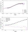 |
Fig. 15. Top: comparison of LoTSS-DR1 differential source counts using “mask d” and SKADS 151 MHz and T-RECS “wide” 150 MHz simulations. The grey band corresponds to a ±20% variation of the LoTSS flux density scale due to uncertainties in the flux density calibration. Bottom: contributions from AGNs and SFGs in the T-RECS “wide” differential source counts as compared to the total LoTSS-DR1 differential source counts. All: error bars are due to Poisson noise in each flux density bin, which have equal bin width in log10(S). |
The sample we choose for the SKADS simulations covers 100 square degrees of the sky, with a minimum flux density of 1 μJy at 1.4 GHz. It contains 6.1 × 10⁶ sources in total, which we consider at a frequency of 151 MHz. There is a small discrepancy in the flux density range from 3 to 12 mJy (see top panel of Fig. 15), otherwise the agreement is excellent down to 0.7 mJy. In the light of the already mentioned 20 per cent error on the flux density calibration, the discrepancy does not seem to be significant.
Three different settings are available from T-RECS for the two main radio source populations (active galactic nuclei and star-forming galaxies). For our source count comparisons, we use the “wide” catalogue, which simulates a sky coverage of 400 square degress with a lower flux density limit of 100 nJy at 1.4 GHz. The T-RECS “wide” catalogue does not include effects of clustering (Bonaldi et al. 2019), while the “medium” T-RECS catalogue does. We checked that this does not result in any significant differences for the differential source counts for the range of flux densities considered in this work. For all T-RECS catalogues frequency bands between 150 MHz and 20 GHz are provided. Here we use the flux densities at 150 MHz. In Fig. 15 the differential source counts of AGNs and SFGs are shown, as well as the sum of both populations. We find that T-RECS is in good agreement with the data of the masked LoTSS-DR1, except for a small discrepancy in the flux density range from 3 to 12 mJy.
5.3. Consistency based on photometric redshift information
As already mentioned in the introduction, a large fraction of LoTSS-DR1 radio sources have identified infrared (72.7%) and optical (51.5%) counterparts, which allow for an estimate of a photometric redshift for around half of LoTSS sources (Duncan et al. 2019). Some of the identified objects also have spectroscopic redshift information available. Below we use the “z_best” redshift information, which is the spectroscopic redshift when it is available and a photometric estimate in all other cases, from the LoTSS-DR1 value-added source catalogue to learn more about the contribution of local structure to the one- and two-point statistics.
The photometric redshifts in the catalogue are extracted from a combination of infrared and optical data from WISE and Pan-STARRS. Due to missing Pan-STARRS information in the strip 55.0000 deg < Dec < 55.2245 deg and RA < 184.4450 deg, we lack photometric redshifts from that strip. The only available data would be redshifts inferred from spectroscopic information of sources that match to a WISE catalogue source. To account for that effect, we additionally mask that strip (see Fig. 5), whenever we use redshift information and will denote this as “mask z”.
Applying cuts in redshift rejects radio sources and the source density per cell decreases significantly. In Table 5 we show how the total number of LoTSS-DR1 value-added sources changes after applying “mask z” for different minimal values of redshift, without and with a flux density threshold of 1 mJy. For about 51% of all radio sources redshift information is available and this number does not change significantly when we restrict the analysis to radio sources with flux densities above 1 mJy.
Number of sources of the masked (mask z) LoTSS-DR1 value-added source catalogue for various flux density thresholds and for different values of minimum redshift z.
The distribution of radio sources with available redshift estimate is shown in Fig. 16 for the four samples with flux density thresholds of 1, 2, 4, and 8 mJy, respectively. The brighter samples show the mode of the distribution at z ≈ 0.7, while the 2 mJy sample is bimodal and the 1 mJy sample has its mode at z ≈ 0.1. The median redshift increases continuously from 0.50 for the 1 mJy to 0.64 for the 8 mJy sample. This is in good qualitative agreement with the expectation (supported also by the simulations discussed above), that the brighter samples are dominated by AGNs at relatively high redshift while in the faintest sample SFGs at lower redshift start to dominate the statistics. First classifications of AGNs and SFGs in the LoTSS-DR1 catalogue have been done by Hardcastle et al. (2019) and Sabater et al. (2019). We additionally separated all sources with available redshift information after masking with “mask z” by the 33 and 66 percentiles, which are:

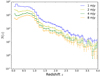 |
Fig. 16. Number of radio sources as a function of available z for four different flux density thresholds, with error bars due to Poisson noise. Only sources with available redshift (“z_best”) of the LoTSS-DR1 value added source catalogue after applying “mask z” are considered here. |
respectively. From these three samples we inferred the differential source counts, which are presented in Fig. 17. These differential source counts support the above expectation, that the source distribution at fainter flux densities is dominated by objects at lower redshift and vice versa at brighter flux densities by objects at higher redshift.
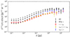 |
Fig. 17. Differential source counts of the LoTSS-DR1 value-added sources masked with “mask z” separated by redshift percentiles, z33 = 0.376 and z66 = 0.705. Additionally the differential source counts of all sources (“All”) and of all sources with redshift information (“Any z”) are shown. |
Radio sources with redshift information are very likely (non-zero probability of misidentification) to be real sources and so we can consider that sample of radio sources as an independently confirmed sample. It is then interesting to compare its statistical properties with those of the sample without redshift information.
In Fig. 18 we show the clustering parameter nc as a function of flux density threshold after applying “mask z”. In the top panel we compare the radio sources with redshift information to those without redshift information. We see that the values for nc agree very well with each other for all considered flux density thresholds. At flux densities below 1 mJy, both sets of sources seem to cluster less than the sum of both sets.
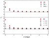 |
Fig. 18. Clustering parameter nc as function of flux density threshold and available redshift information based on the value “z_best” from the LoTSS-DR1 value-added source catalogue after application of “mask z”. Top: we compare radio sources with and without redshift information and contrast them with the full sample. Bottom: only objects with redshifts above the quoted value are included in the respective data points. Error bars are computed from bootstrap sampling. |
We also show in the bottom panel of Fig. 18 how nc changes when we exclude all sources estimated to be below a certain redshift. Interestingly, we find that excluding radio sources from the local neighbourhood (z < 0.2) decreases the clustering parameter nc. The effect increases if we exclude radio sources from a larger volume and is strongest if we exclude all objects in the local Hubble volume (z < 1). This effect is seen for all flux density thresholds, but is most prominent for thresholds below 1 mJy. This is consistent with the expectation that there is more clustering in the late Universe, but a much more detailed study will be necessary to make quantitative statements, which we leave for a future work. We dismiss radio sources below 1 mJy in the following section when we study the two-point correlation function.
We conclude our study of the one-point statistics by pointing out that LoTSS-DR1 produces reliable radio source counts and shows statistical properties that are self-consistent and consistent with previous observations and simulations above integrated flux densities of 1 mJy. The corresponding counts-in-cell map for “mask d” and “mask 1” with S > 1 mJy is shown in Fig. 19.
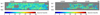 |
Fig. 19. Counts-in-cell map of the LoTSS-DR1 value-added source catalogue for S > 1.0 mJy and after applying “mask d” (left) and “mask 1” (right). |
6. Two-point statistics
6.1. The angular two-point correlation function
In order to estimate the angular two-point correlation of radio sources, we make use of the estimator proposed by Landy & Szalay (1993),
where DD, DR, and RR denote the normalised pair counts at separation angle θ for data-data, data-random, and random-random source pairs (see Appendix B for details). The Landy-Szalay (LS) estimator has minimal bias and minimal variance and is claimed to be more robust than other estimators (see Kerscher et al. 2000 and Appendix B). Data points are taken from the LoTSS-DR1 value-added source catalogue and random points either from the mock catalogue (default) described in Sect. 4, or from a purely random sample. Data and random catalogues are masked alike.
For a large enough random source catalogue, the expectation value of the LS estimator is (Landy & Szalay 1993):
where wΩ = ∫Gp(θ)w(θ)dθ, with Gp(θ) being the normalised count of pairs of “atomic” cells (cells that are small enough to contain at most one point source) at separation θ in the analysed survey area. Thus, the LS estimator (as well as all other estimators that have been proposed in the literature) is biased. The function Gp(θ) depends on the binning.
The bias of the estimator is due to the so-called integral constraint, which is an effect of the finite survey area and reflects the fact that we cannot measure an unbiased estimate of the two-point correlation based on a single estimate of the total number of sources in the survey region. Given a model for w(θ), we can estimate this bias from the random source catalogue via:
The variance of the estimator is (Landy & Szalay 1993)
![$$ \begin{aligned}&\mathrm{Var} [\hat{w}(\theta )] = \left(\frac{1+w(\theta )}{1+w_\Omega }\right)^2 \frac{2}{N_\mathrm{d} (N_\mathrm{d} -1) G_\mathrm{p} (\theta )} \end{aligned} $$](/articles/aa/full_html/2020/11/aa36592-19/aa36592-19-eq42.gif)
where Nd denotes the number of data points in the survey. The second expression holds for the assumption that the two-point correlation is small compared to unity. The factor Nd(Nd − 1)/2 scales the Poisson noise with the overall number of pairs and the factor Gp(θ) accounts for how many independent pairs can be probed at angular separation θ.
For calculating the correlations, we make use of the publicly available code TREECORR6 in version 3.3 (Jarvis et al. 2004). TREECORR uses an algorithm that structures the sources in cells according to a logarithmic binning of cell separation. In that way, the numerical problem of calculating the two-point correlations for objects in cells with N1 and N2 members is reduced from scaling with 𝒪(N1N2) to 𝒪(N1 + N2), which leads to a huge speed-up compared to a naive algorithm. As it is advised to use mock catalogues that are much larger than the data catalogues, the computational time scales linearly with the number of mock sources considered. Using TREECORR, we fix the range to 0.1 deg ≤θ ≤ 32 deg with equal bin width of Δln(θ/1 deg) = 0.1. In order to account for the shot noise in samples with smaller numbers of sources, we increase the bin width by factors of two. The bin centres are estimated by using the mean value of ln(θ/1 deg) for all pairs in the bin. The TREECORR parameter bin_slop controls the accuracy of the computation. It turns out that one must take care to change its default setting to obtain the required accuracy once the two-point correlations are at or below 𝒪(10−2), as discussed and demonstrated in some detail in Appendix C. bin_slop=0 gives the best possible result. It should also be stressed that for angles exceeding a few degrees it is important to compute angular distances on great circles, which is achieved by setting the TREECORR parameter metric = “Arc”. We have verified that using the Euclidean metric instead makes a noticeable difference at the largest angular scales accessible in LoTSS-DR1.
We base our analysis on the LoTSS-DR1 value-added source catalogue. We start our analysis with “mask d” and flux density thresholds of 1, 2, and 4 mJy. At flux density thresholds larger than 1 mJy we expect the point source completeness to be well above 99 per cent. We also apply corresponding flux density thresholds on the mock catalogue (Sect. 4), which then contains 1 923 339, 995 218, and 545 520 mock sources for “mask d” and 798 490, 412 922, and 226 385 mock sources for “mask 1”, respectively.
The angular two-point correlation function w(θ) with statistical errors calculated by TREECORR is shown in Fig. 20 for different flux density thresholds. The error estimation of TREECORR is based on the Poisson noise in each separation bin. We additionally tested error estimations in terms of bootstrapping and found no large difference in both estimations, see Appendix C for details. Previous radio continuum surveys showed larger bootstrap errors than Poisson errors, see Cress et al. (1996) for the FIRST survey. They found the Poisson error to be less than the bootstrap estimate by a factor of two for small scales around θ ∼ 0.05 deg and even larger for increasing separations. The geometry of the survey provides an increasing number of correlation weighted pair counts up to angular separations of θ < 6 deg, at larger angular separations the weighted pair counts decrease and finally drop steeply at 30 deg. In the figures we shade angular scales θ > 6 deg in grey.
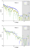 |
Fig. 20. Angular two-point correlation of sources from the LoTSS-DR1 value-added source catalogue after masking with “mask d” (top) and “mask 1” (bottom) and at flux densities above 1, 2, and 4 mJy. Positive and negative values are shown with full and open symbols, respectively. The grey shaded region indicates angular separations with decreasing number of weighted pair counts. |
In the top panel of Fig. 20, we observe consistent behaviour for all three flux density samples above three degrees. Below three degrees the 1 mJy sample is more correlated than the 2 and 4 mJy samples, which are more consistent. However, it can be seen that there are many angular bins in which the 4 mJy sample shows a low value of the two-point correlation function. We believe this is likely as a result of having fewer sources in that sample. The bottom panel of that figure explores what happens if we restrict our analysis to the low-noise region of the survey after applying “mask 1” (see Sect. 3.5). Now all three samples are more consistent with each other. However, the number of sources has been reduced by about a factor of two in each sample.
The observed increase of correlation for decreasing flux density thresholds in “mask d”, which is not observed in the low-noise region of “mask 1”, is investigated further. Particularly, we ask if flux dependent correlation is related to the method of generating the mock catalogue, as it relies on the local noise patterns. To do so, we measure the correlation function of the mock catalogue itself, by comparing to a pure random sample (spatial Poisson process). In Fig. 21, we see that there is almost a vanishing mock auto-correlation (denoted mock-random in the legend) above the typical size of an individual pointing (1.7 deg in radius), whereas for smaller angular separations the correlation is an order of magnitude smaller than that of the data sample. We also show in Fig. 21 the data-mock and data-random (spatial Poisson process) auto-correlations. The data-mock and data-random results agree at all scales with small differences. This also holds true for the three different masks “1”, “2”, and “d”, which we have tested separately. The close similarity of results based on pure random samples and the mock catalogue shows that the flux density dependence of the observed correlations is not a result of how we generate the mock catalogue. We also see from Figs. 20 and 22 that the reduced noise level of “mask 1” increases the correlation for the 2 and 4 mJy samples, but does not change the 1 mJy sample significantly.
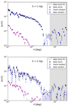 |
Fig. 21. Comparison of two-point angular (auto-)correlation functions for “mask d” for different random catalogues: mock catalogue based on LoTSS local rms noise (data-mock), homogeneous random catalogue accounting for survey geometry only (data-random), and the correlation of the mock catalogue (mock-random) for flux densities above 1 mJy (top) and 2 mJy (bottom). We fitted the data to the power-law model described in the text. Positive and negative values are shown with full and open symbols, respectively. The grey shaded region indicates angular separations with decreasing number of weighted pair counts. |
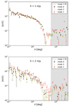 |
Fig. 22. Angular two-point correlation from the LoTSS-DR1 value-added source catalogue after masking with “mask d”, “mask 1”, and “mask 2” at flux densities above 1 mJy (top) and 2 mJy (bottom) for data-mock pairs; see caption of Fig. 21 for further details. We fitted the data of “mask 1” to the power-law model described in the text. Positive and negative values are shown with full and open symbols, respectively. The grey shaded region indicates angular separations with decreasing number of weighted pair counts. |
Whilst the procedure of generating mocks (Sect. 4) does account in the large sense for the inhomogeneity of completeness (see e.g. Figs. 3 and 9), it may have completeness issues close to the five-sigma detection threshold. This could be due to a variety of reasons such as completeness when using PYBDSF to detect sources (which is not used for the randoms); the assumption of point sources when generating randoms and finally flux scale issues within the data. However, when applying flux thresholds that are significantly above the averaged 95% completeness flux density of 0.39 mJy, variations in completeness should not affect our results at a significant level.
To further investigate the origin of the flux density dependence of the angular two-point correlation, we perform a jack-knife test and split up the survey into three regions on the sky, namely “Right”, “Center”, and “Left”. These lie within the following right ascension intervals: [161, 184], (184, 208], (208, 230] deg, respectively. We then compute w(θ) and errors as mentioned above and compare the results, shown in Fig. 23 for the 1 and 2 mJy samples of “mask d” and in Fig. 24 for “mask 1”. We observe for the 1 mJy sample of “mask d” that the angular two-point correlation functions of the three regions agree at the smallest angular separations, but show significantly less correlation for the central region as compared to the left and the right region at scales around 1 deg. The reason for this discrepancy is not fully understood, we think it may be due to issues in the flux density calibration of individual pointings.
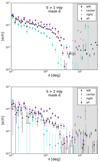 |
Fig. 23. Angular two-point correlation function of sources from the LoTSS-DR1 value-added source catalogue with “mask d” and flux density threshold of 1 mJy and 2 mJy, for three regions namely “Left”, “Center”, and “Right”. |

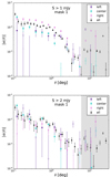 |
Fig. 24. Angular two-point correlation function of sources from the LoTSS-DR1 value-added source catalogue with “mask 1” and flux density threshold of 1 mJy and 2 mJy, for three regions namely “Left”, “Center”, and “Right”. |

The hypothesis of a fluctuation in the flux density calibration is supported by the observed lack of source counts south of the unobserved hole in the HETDEX field. To see that, we compare the LoTSS-DR1 radio source catalogue (Fig. 1) and the mock catalogue (Fig. 9). According to the mock catalogue, which is based on the local rms noise (Fig. 7), we should see an overdense region, whereas the actual source counts reveal an underdensity. Also the completeness map (Fig. 2) supports the findings from the mock catalogue. An underestimation of the flux scales in the corresponding pointings would give rise to exactly that effect. It would lead to smaller observed flux densities, which would lead to less observed sources close to the detection limit, but in terms of noise to cleaner and more complete regions. A simple model for the flux calibration assumes a linear relation between the true flux scale and the actual flux scale used in each pointing, Sp = cpStrue + op, where cp is fixed observing one or several calibrator sources for each particular pointing. For large enough flux densities, the offset op, which is expected to be at least of the order of the rms noise, is irrelevant, but becomes relevant close to the detection threshold. Consequently, samples with increased flux density threshold are less affected by flux density calibration offsets.
For the 2 mJy sample of “mask d”, the right region is consistent with the full sample, whereas the left region shows an increased correlation and the central region a decreased correlation. We note that the left region has the most complicated geometry. The interpretation of Fig. 23 is complicated by different values of wΩ for the three different regions, due to their different survey geometry and sky coverage. We conclude that the 2 mJy sample shows a more self-consistent behaviour as compared to the 1 mJy sample. However, the differences in the angular two-point correlation function that occur in different regions within the field at 2 mJy are not well understood. It is hoped that this will be reduced with the next data release of the LoTSS survey, where there will be a larger sky coverage and, if there are flux scaling issues, these flux scaling issues may be reduced. The results of the jack-knife test within different spatial regions are consistent with the idea that differences relate to the flux-density calibration of individual pointings, as the 2 mJy sample is affected to a lesser extent than the 1 mJy sample.
In the jack-knife of the 1 mJy “mask 1” sample we observe consistently less correlation in the left part of the survey than in the right part. The central region shows consistent behaviour at small scales with the left part and starts to deviate from it at scales ∼1 deg. As seen previously for “mask d”, the full sample shows correlation in between the three parts, as it is a combination of the three parts. Comparing the sky coverage of “mask d” and “mask 1” in Fig. 8 the left part is affected most by cutting in the local noise per cell.
For the 2 mJy sample of “mask 1”, we find consistent behaviour for all three parts and also consistent behaviour with the full sample. Outliers and even negative correlations mostly seen in the left part can be explained by the highly decreased number of sources in this sample, which leads to higher contributions of shot noise.
Comparing the jack-knife test for “mask d” and “mask 1”, we consider the results of “mask 1” to be more consistent and not as affected by flux calibration variations as in the case of “mask d”, especially in the case of the 2 mJy sample. Therefore we will use the “mask 1” 2 mJy sample as the default sample for our future analysis.
In order to ease the comparison between different samples and with angular two-point correlation functions published elsewhere (Kooiman et al. 1995; Rengelink et al. 1999; Blake & Wall 2002; Overzier et al. 2003; Blake et al. 2004; Rana & Bagla 2019; Dolfi et al. 2019), we fitted the data points in Fig. 20 to a power-law model of the form:
The value of such a power-law fit for a cosmological analysis is limited, as it holds at best for a small range of angular scales. For fitting we make use of the publicly available Python LMFIT7 package (Newville et al. 2016), where we used the default Levenberg-Marquardt method. We fitted the data points in the range of 0.2 ≤ θ ≤ 2.0 deg. We then explicitly compute wΩ using Eq. (28) from the initial fit parameters and re-do the fitting but this time by selecting only those data points which are greater than wΩ. The entire process is re-iterated until stable values for A, γ, and wΩ are obtained. Best-fit results obtained in such a manner are summarised in Table 6 and are shown in Figs. 21 and 22. This procedure is done for the 1, 2, and 4 mJy flux density thresholds with “mask d”, as well as for “mask 1”.
Best-fit values of w(θ) = A(θ/1 deg)−γ, fitted in the range 0.2 ≤ θ ≤ 2.0 deg and corresponding integral constraint wΩ for the LoTSS-DR1 value-added source catalogue after appropriate masking and for the TGSS-ADR1 catalogue, with 68% confidence intervals.
We find that the values of A and γ depend on the detailed cuts and flux density thresholds applied. Higher flux density threshold means smaller correlation amplitude in case of “mask d”, which is contrary to the findings of Wilman et al. (2003) in terms of the Boötes Deep Field and Rana & Bagla (2019) in terms of the TGSS-ADR1. This difference may reflect issues arising from flux scale issues which, as mentioned previously, may be affecting the results presented in this work and should be improved using the next data release of the LoTSS survey. Alternatively, this may reflect the changing distribution of populations at different flux density limits within our samples as we will have a larger fraction of SFGs at lower flux density limits. This could make direct interpretation of the clustering amplitude difficult as the SFG and AGN are thought to have different bias measurements (Magliocchetti et al. 2017; Hale et al. 2018) and will have different redshift distributions. In Table 6, we also provide the goodness-of-fit in terms of χ2 over number of degrees of freedom. “mask 1” and “mask d” agree on goodness-of-fit and the best-fit values of A and γ for 1 and 2 mJy within three sigma. However, the two values for the 4 mJy sample are inconsistent with each other, but the “mask 1” measurement suffers from a rather small number of sources. Based on the various tests reported above, we conclude that the most reliable measurement is obtained by “mask 1” for the 2 mJy sample: A = (5.1 ± 0.6) × 10−3 and γ = 0.74 ± 0.16.
This result can be compared to angular two-point correlation functions reported in the literature. For the NVSS A = (1.49 ± 0.15) × 10−3, γ = 1.05 ± 0.10 from Blake et al. (2004) at SNVSS > 10 mJy and A = (1.0 ± 0.2) × 10−3 for γ = 0.8 from Overzier et al. (2003) at same flux density threshold. Results found for lower frequencies in the WENSS survey, for example, A = (2.0 ± 0.5) × 10−3 for γ = 0.8 from Rengelink et al. (1999) and A = (1.01 ± 0.35) × 10−3, γ = 1.22 ± 0.33 from Blake et al. (2004) at SWENSS > 35 mJy. Results in the same frequency range as LoTSS have been obtained from the TGSS-ADR1 catalogue and are shown in Table 6. Thus the slope found in LoTSS-DR1 is consistent with the findings for TGSS-ADR1 at much higher flux densities, but differs from the slope found at higher frequencies. The amplitude found in LoTSS-DR1 is smaller than the one found for TGSS-ADR, but larger than the one from NVSS and WENSS.
6.2. The angular two-point correlation function for redshift sub-samples
We further make use of the available redshift information in the LoTSS-DR1 catalogue, namely the “z_best” values. We first divide the LoTSS-DR1 catalogue into two sub-samples based on the information whether a “z_best” value for a given radio source is available or not. We then compute the angular two-point correlation function for the sub-sample with redshift information, called “Any z”, which is shown in Fig. 25 for “mask z” (top). As the results of Sect. 6.1 show more consistent results for “mask 1” than for “mask d”, we additionally generate a redshift mask for the region of “mask 1”, which is denoted as “mask z1”. The results for the angular two-point correlation with “mask z1” are shown in Fig. 25 (bottom). Based on the strong difference between the angular two-point correlation of the 1 and 2 mJy samples of “mask d”, we neglect the 1 mJy in the further analysis.
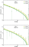 |
Fig. 25. Comparison of the angular two-point correlation function estimated from the LoTSS-DR1 value-added source catalogue for radio sources with redshift information and theoretical expectations (solid lines) for the best-fit ΛCDM cosmological parameters from Planck, generated using CAMB SOURCES with Halofit and b(z) from Eq. (28). The integral constraint wΩ is computed for the expectations and subtracted from them. Positive values are shown with full symbols and solid lines, whereas negative values are shown with open symbols and dashed lines. |
Additionally, we test different redshift sub-samples defined in Eq. (25) in Sect. 5.3, where the survey is split up into three parts, namely z1: z < z33, z2: z33 ≤ z < z66, and z3: z66 ≤ z. These parts are separated by the 33 and 66 percentiles, defined in terms of the survey without any flux density thresholds and are kept the same for higher flux density thresholds. The measured angular two-point correlations for a flux density threshold of 2 mJy, masked with “mask z” for the three redshift bins are presented in Fig. 26. Due to the strongly decreased number of sources per bin in the 2 mJy samples, we increased the bin width to Δln(θ/1 deg) = 0.4.
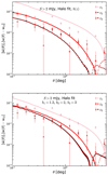 |
Fig. 26. Angular two-point correlation function for three redshift bins z1, z2 and z3 for a flux density threshold of 2 mJy. The lines show the expectations for the cosmological standard model. Both panels use the Halofit option of CAMB SOURCES, which accounts for the non-linear evolution of large scale structure. In the top panel we use the bias function of Eq. (32), whereas we use a piecewise constant bias in the bottom panel. The integral constraint wΩ is computed for the expectations and subtracted from them. Positive values are shown with full symbols and solid lines, whereas negative values are shown with open symbols and dashed lines. |
Fitting a power law, as defined in Eq. (31), gives the results shown in Table 6. We can see that the goodness-of-fit is close to one, except for the first redshift bin. We see stronger correlation for most of the redshift bins, which is expected as there is less smearing. The exponent γ and the amplitude A are larger as compared to the best-fit LoTSS-DR1 2 mJy “mask 1” sample and to the NVSS values. And the amplitudes increase further if we consider individual bins in redshift as compared to the study that includes any value of the redshifts.
However, a disclaimer is in order: We did not estimate and propagate errors on the redshift estimation. Thus, the error bars shown assume that the redshift estimates used here are exact. We expect that the errors for the “Any z” sample are nevertheless realistic, as only the fact is used that those sources have optical and infrared counterparts and the photometric redshift estimator found a solution. But when we split up the radio sources with photometric redshift into three bins, the reliability of the redshift estimate becomes an issue. It is well known that there is a finite and non-negligible probability that AGNs from bin z3 would be misestimated and end up as sources in bin z1, see Duncan et al. (2019). Propagating this effect through our analysis pipeline and correcting for it was beyond the scope of this work. Since only half of the LoTSS-DR1 radio sources have redshift information available, it is currently impossible to measure the bias evolution of the complete sample. We also note that due to only half of the sources having redshifts available, there will be underlying selection effects in these sub-samples that may not necessarily represent the full sample as a whole.
6.3. Comparison of angular two-point correlations to expectation of cosmological standard model
In order to compare our measured angular two-point correlation function to expectations, we rely on the publicly available CAMB SOURCES code (Challinor & Lewis 2011) to calculate the angular power spectrum Cl for 2 ≤ l ≤ 4000. From this power spectrum we infer the two-point correlation function w(θ) by using Eq. (14). In doing so, we assume a vanishing monopole and dipole. The theoretical monopole vanishes by definition and the theoretically expected dipole is the sum of a structure dipole and the kinematic dipole (Ellis & Baldwin 1984) caused by the proper motion of the Solar system. We have checked with a simulation that the survey area of LoTSS-DR1 would pick up that dipole at a level that is about an order of magnitude below the actually observed signal and we thus neglect the dipole contribution in this analysis (see Appendix D for further details). The dipole contribution will become more important at larger angular separations for larger survey areas (Bengaly et al. 2018).
In order to predict the angular two-point correlation, we have to specify a cosmological model, the redshift distribution of the observed sources and how well they trace the underlying matter density distribution, which is expressed as a bias function. We fix the cosmological parameters to the best-fit ΛCDM cosmology of the Planck 2018 analysis (Planck Collaboration VI 2020; Planck Collaboration I 2020), which are the Hubble rate today (H0), the dimensionless, Hubble independent baryon density (Ωbh2) and cold dark matter density (Ωch2) with h = H0/(100kms−1 Mpc−1), the primordial amplitude of curvature perturbation (As) and the spectral index of curvature perturbation (ns) with their recent best-fit values:
The optical depth, which is usually also reported, is of no concern for the prediction of the angular power spectrum of matter. The redshift distribution of radio sources is estimated from the histogram of the measured photo-z from the LoTSS-DR1 value-added source catalogue, shown in Fig. 16, which is used as source window function for the three different flux density threshold samples. For the galaxy bias, b(z), we use a parametrisation introduced by Nusser & Tiwari (2015), Tiwari & Nusser (2016) as a fit to NVSS data:

which was adapted by Bengaly et al. (2018) and Dolfi et al. (2019) in the context of TGSS data. The CAMB package allows to include the effects of gravitational lensing and it allows users to include effects of non-linear structure formation via its halo-fit option (Takahashi et al. 2012; Mead et al. 2015). Additionally, we do not use the Limber approximation, which is per default used for l > 100. An inappropriate application of the Limber approximation gives rise to ringing phenomena in w(θ) that depend on the details of the binning of the redshift distribution function. We make use of the cubic-spline interpolation of CAMB to generate a smooth window function from the observed redshift distribution for sources with z ≤ 2.
In Fig. 25 we show the two-point correlations from radio sources with available redshift information for the 2 and 4 mJy flux density thresholds and compare them to the predictions of non-linear theory, including the Halofit and count lensing options of the CAMB package and the bias from Eq. (32). In order to account for the integral constraint, we calculate it using Eq. (28) with the random-random pairs obtained by TREECORR and the expectation from CAMB in order to subtract it from the expectation. We find reasonable agreement for angular separations below a few degrees, for the 2 and 4 mJy samples of “mask z”, as well as of “mask z1”. The agreement between the theoretical expectations and the results for the 2 and 4 mJy samples is remarkable as we did not adjust any model parameter.
Besides varying the flux density threshold, we can also put the data into several redshift bins, as done previously in Sect. 5.3 and 6.2, which allows us to test the bias model in more detail. We compare two scenarios for the 2 mJy “mask z” sample only, as the angular two-point correlation behaves similarly for “mask z” and “mask z1”. For the first scenario we use of the Halofit option of CAMB, together with the bias function b(z) and include the effect of lensing. We see in the top-left panel of Fig. 26 that the CAMB predictions for redshift bin z1 overestimate the amount of correlation while we obtain a reasonable agreement for the z2 bin at smallest angular scales and for z3 below ∼0.8 degrees. A possible explanation is that the bias function (32), which is based on NVSS data, overestimates the amount of bias at lower redshifts for a population mix that includes many more SFGs compared to NVSS.
In order to test this hypothesis, we compute a second scenario, where we use a constant bias b(z1) = b1 = 1.2 for the z1 bin, make use of the Halofit option of CAMB and include lensing. Doing so, the expectation of the first redshift bin is in better agreement below 2 deg with the estimated two-point correlation function. This indicates that LoTSS-DR1 radio sources at small photometric redshift are almost unbiased tracers of the large scale structure, which is to be expected if the sample is dominated by SFGs (which are thought to or assumed to have smaller bias, see, for example, the models used in Wilman et al. 2008 and results from Hale et al. 2018). This also may relate to selection effects of which sources have associated redshifts, which may preferentially select low redshift SFGs over higher redshift AGN. We also use a piecewise constant bias of b2 = 2 and b3 = 3 for the redshift bins z2 and z3 respectively, which also improve the match of the expectations to the estimated two-point correlation function.
A more detailed study including the precise measurement of the bias functions and cosmological parameters like σ8 are beyond the scope of this work, as a good understanding of the uncertainties of the photometric redshift distribution is needed to do so.
7. Conclusions
We have presented the first statistical analysis of the spatial distribution of radio sources from LoTSS, based on the observation of 424 square degrees of the sky. We did so in order to characterise the global properties of the survey, check the quality of the LoTSS-DR1 catalogues and test whether upcoming data releases will provide promising opportunities to probe cosmology. We achieved all three of those goals.
The data quality was assessed by a suite of tests on top of those already presented in Shimwell et al. (2019) and Williams et al. (2019). We measured the point-source completeness of the survey and found it to be complete to better than 99 per cent above a flux density of 1 mJy. We demonstrated that in the mean, source counts are independent from the distance from the pointing centre out to an angular separation of approximately 1.6 deg, which corresponds almost to the average effective pointing radius of 1.7 deg, although showing sizeable variation in the counts between pointings, see Fig. 4. We also showed that source counts around the five brightest objects (i.e. > 10 Jy) in the LoTSS-DR1 value-added source catalogue do not show a statistically significant deficit of sources, though they are at the lower end of the spread of source counts. Combined with our results for point-source completeness, we conclude that LoTSS-DR1 allows us to probe the radio sky over more than four orders of magnitude in flux density. We also demonstrated that the statistical moments of the counts-in-cells distribution of the LoTSS-DR1 value-added source catalogue with only the five most incomplete pointings and a handful of pixels with less than 5 sources removed, are in excellent agreement with those from the LoTSS-DR1 radio source catalogue masked with our most aggressive noise mask that restricts the analysis to low-noise cells (below the median cell-averaged rms noise). This assures us of the excellent quality of the pipeline described in detail in Williams et al. (2019) and Duncan et al. (2019) to construct the value-added source catalogue.
The next step was to measure the statistical moments of the distribution of the radio sources in various aspects. We tested if the counts-in-cell tests show any indication of clustering or if they agree with a Poisson distribution, the most naive expectation for any sky survey. We can exclude with very high confidence that the counts-in-cell are consistent with a Poission distribution. The counts-in-cell statistics show a clear signature of clustering, quantified by the clustering parameter nc, which is a proxy for the number of cluster members. Comparing the radio source catalogue and the value-added source catalogue, in which many multi-component sources have been identified and assigned to a single radio source and many artefacts have been removed, shows a significant difference in nc and also in higher statistical moments. We note that as one increases the flux density threshold, the deviation from a Poisson distribution becomes smaller. However, for S > 10 mJy and the available 424 square degrees of survey area the counts per cell become so small that measuring a deviation from a Poisson distribution is difficult.
For the value-added source catalogue, we showed that the simplest compound Poisson distribution in which each cluster contains a random number of objects that are again Poisson distributed fits the data very well. A possible explanation for that finding is that this is due to multiple component radio sources, but here the reader should be aware that the statistical test is not able to distinguish real multi-component sources, such as lobes of radio galaxies, from a SFG with a radio artefact in its vicinity or a group of SFGs. As the deviation from the Poisson distribution is strongest below flux densities of 1 mJy, it is unlikely that all of the clustering is due to real radio sources, at least some of that clustering might still be due to artefacts, as presumably the reliability of the LoTSS-DR1 value-added source catalogue reduces when the noise level is approached. This hypothesis is also supported by the reduction of nc when only sources with photometric redshift information are used in the data analysis. Presumably, fluctuations of the flux density scale between individual pointings also give rise to deviations from a Poissonian source distribution. A significant increase of the number of pointings in DR2 will allow us to study this issue in detail. The clearly detected deviation from the Poisson distribution suggests an additional contribution to the observed large variance of counts of sub-mJy radio sources at higher frequencies, additional to cosmic variance and sample variance (Heywood et al. 2013).
We further studied the differential source counts of LoTSS-DR1 and compared them to other data at low radio frequencies. They are in good agreement above 1 mJy and follow the expectations from the SKADS and T-RECS simulations. The photometric redshift estimates for about half of all radio sources obtained from crossmatching with optical and infra-red observations allow us to get a first impression of the redshift distribution of the LoTSS-DR1 sample. It will be important to figure out how representative they are also for the other half of the sample. An important step forward in that respect will be the WEAVE-LOFAR survey, which will obtain about a million spectroscopic redshifts.
We also estimated the angular two-point correlation of the LoTSS-DR1 value-added sources in Sect. 6. Different flux density thresholds and masking strategies lead to slightly varying results. We conclude that the 2 mJy sample from low-noise regions (mask 1) is the most reliable sample. We find less correlation than in the analysis of TGSS-ADR data (Rana & Bagla 2019; Dolfi et al. 2019) on all scales accessible by LoTSS-DR1, see also Fig. A.2.
We finally used the distribution of photometric redshifts for about half of all LoTSS-DR1 value-added sources to also compare to the Planck 2018 best-fit cosmology, using an off-the shelf bias model and a piecewise constant bias model. For the angular scales below 6 degrees, we find relatively good agreement between our measurements and the expectation (no fitted parameters) for the 2 and 4 mJy samples. A more detailed comparison that also makes use of binned redshift information reveals problems with the bias model of Tiwari & Nusser (2016) especially at low redshifts, which is likely due to the fact that we do not account for the difference between AGNs and SFGs in that analysis.
To conclude, we recover that the radio sky is statistically isotropic at better than one per cent at angular scales above 1 deg and we find that large-scale structures as probed with a subset of LoTSS-DR1 sources that have photometric redshifts and a flux density limit of 2 mJy, are relatively consistent with the Planck 2018 best-fit cosmology at angular scales below 6 degrees (see Fig. 25). A measurement of cosmological parameters was beyond the scope of this work. A next step will be to improve the consistency of the flux density calibration and to quantify and estimate the errors of the measured distribution of photometric redshifts. With those two elements improved, in combination with a vastly improved imaging pipeline for DR2 and a much larger sky coverage of 5700 square degrees, we expect that we will start to be able to make interesting cosmological tests and measure cosmological parameters based on LoTSS radio sources.
Acknowledgments
This paper is based on data obtained with the International LOFAR Telescope (ILT) under project codes LC2_038 and LC3_008. LOFAR (van Haarlem et al. 2013) is the Low Frequency Array designed and constructed by ASTRON. It has observing, data processing, and data storage facilities in several countries, which are owned by various parties (each with their own funding sources), and which are collectively operated by the ILT foundation under a joint scientific policy. The ILT resources have benefited from the following recent major funding sources: CNRS-INSU, Observatoire de Paris and Université d’Orléans, France; BMBF, MIWF-NRW, MPG, Germany; Science Foundation Ireland (SFI), Department of Business, Enterprise and Innovation (DBEI), Ireland; NWO, The Netherlands; The Science and Technology Facilities Council, UK; Ministry of Science and Higher Education, Poland; The Istituto Nazionale di Astrofisica (INAF), Italy. This research made use of the Dutch national e-infrastructure with support of the SURF Cooperative (e-infra 180169) and the LOFAR e-infra group. The Jülich LOFAR Long Term Archive and the German LOFAR network are both coordinated and operated by the Jülich Supercomputing Centre (JSC), and computing resources on the supercomputer JUWELS at JSC were provided by the Gauss Centre for Supercomputing e.V. (grant CHTB00) through the John von Neumann Institute for Computing (NIC). This research made use of the University of Hertfordshire high-performance computing facility and the LOFAR-UK computing facility located at the University of Hertfordshire and supported by STFC [ST/P000096/1], and of the Italian LOFAR IT computing infrastructure supported and operated by INAF, and by the Physics Department of Turin university (under an agreement with Consorzio Interuniversitario per la Fisica Spaziale) at the C3S Supercomputing Centre, Italy. This research made use of Astropy, a community-developed core Python package for astronomy (Astropy Collaboration 2013) hosted at http://www.astropy.org/, and of the astropy-based reproject package (http://reproject.readthedocs.io/en/stable/). Some of the results in this paper have been derived using the healpy (Zonca et al. 2019) and HEALPIX (Górski et al. 2005) package. This research made use of DS9 (Joye et al. 2003), TOPCAT (Taylor 2005), matplotlib (Hunter 2007), NumPy (Walt 2011), SciPy (Virtanen et al. 2020), TREECORR (Jarvis et al. 2004) and tqdm (da Costa-Luis 2019). We thank Mike Jarvis for providing details on TREECORR and Anna Bonaldi for discussions on T-RECS results. We thank Aritra Basu for useful comments and discussions. M. B., N. B., T. M. S. and D. J. S. acknowledge the Research Training Group 1620 “Models of Gravity”, supported by Deutsche Forschungsgemeinschaft (DFG) and by the German Federal Ministry for Science and Research BMBF-Verbundforschungsprojekt D-LOFAR IV (Grant number 05A17PBA). C. L. H. acknowledges funding support from the Science and Technology Facilities Council (STFC) for a PhD studentship [ST/N504233/1]. D. B. acknowledges funding from STFC Grant [ST/N000668/1]. The Leiden team acknowledges support from the ERC Advanced Investigator programme NewClusters 321271. MJH acknowledges support from STFC [ST/R000905/1]. PNB and JS are grateful for support from the UK STFC via grant ST/R000972/1. G. J. W. gratefully acknowledges support of an Emeritus Fellowship from The Leverhulme Trust. WLW also acknowledges support from the CAS-NWO programme for radio astronomy with project number 629.001.024, which is financed by the Netherlands Organisation for Scientific Research (NWO).
References
- Amendola, L., Kunz, M., & Sapone, D. 2008, J. Cosmol. Astro-Part. Phys., 2008, 013 [NASA ADS] [CrossRef] [Google Scholar]
- Astropy Collaboration (Robitaille, T. P., et al.) 2013, A&A, 558, A33 [NASA ADS] [CrossRef] [EDP Sciences] [Google Scholar]
- Ballardini, M., & Maartens, R. 2019, MNRAS, 485, 1339 [CrossRef] [Google Scholar]
- Bengaly, C. A. P., Maartens, R., & Santos, M. G. 2018, J. Cosmol. Astro-Part. Phys., 2018, 031 [NASA ADS] [CrossRef] [Google Scholar]
- Bengaly, C. A. P., Siewert, T. M., Schwarz, D. J., & Maartens, R. 2019, MNRAS, 486, 1350 [NASA ADS] [CrossRef] [Google Scholar]
- Berlind, A. A., & Weinberg, D. H. 2002, ApJ, 575, 587 [NASA ADS] [CrossRef] [Google Scholar]
- Biermann, M. 2019, Master’s Thesis, Bielefeld University, Bielefeld, Germany [Google Scholar]
- Blake, C., & Wall, J. 2002, MNRAS, 337, 993 [NASA ADS] [CrossRef] [Google Scholar]
- Blake, C., Mauch, T., & Sadler, E. M. 2004, MNRAS, 347, 787 [NASA ADS] [CrossRef] [Google Scholar]
- Bonaldi, A., Bonato, M., Galluzzi, V., et al. 2019, MNRAS, 482, 2 [NASA ADS] [CrossRef] [Google Scholar]
- Camera, S., Santos, M. G., Bacon, D. J., et al. 2012, MNRAS, 427, 2079 [CrossRef] [Google Scholar]
- Challinor, A., & Lewis, A. 2011, Phys. Rev. D, 84, 043516 [NASA ADS] [CrossRef] [Google Scholar]
- Chevallier, M., & Polarski, D. 2001, Int. J. Mod. Phys. D, 10, 213 [NASA ADS] [CrossRef] [Google Scholar]
- Condon, J. J. 1988, in Radio Sources and cosmology, eds. K. I. Kellermann, & G. L. Verschuur, 641 [Google Scholar]
- Condon, J. J., Cotton, W. D., Greisen, E. W., et al. 1998, AJ, 115, 1693 [NASA ADS] [CrossRef] [Google Scholar]
- Cress, C. M., Helfand, D. J., Becker, R. H., Gregg, M. D., & White, R. L. 1996, ApJ, 473, 7 [NASA ADS] [CrossRef] [Google Scholar]
- da Costa-Luis, C. 2019, J. Open Source Softw., 4, 1277 [CrossRef] [Google Scholar]
- Dalal, N., Doré, O., Huterer, D., & Shirokov, A. 2008, Phys. Rev. D, 77, 123514 [NASA ADS] [CrossRef] [Google Scholar]
- Dalton, G., Trager, S. C., Abrams, D. C., et al. 2012, SPIE Conf. Ser., 8446, 84460P [Google Scholar]
- Dalton, G., Trager, S., Abrams, D. C., et al. 2014, SPIE Conf. Ser., 9147, 91470L [Google Scholar]
- Davis, M., & Peebles, P. J. E. 1983, ApJ, 267, 465 [NASA ADS] [CrossRef] [Google Scholar]
- de Gasperin, F., Intema, H. T., & Frail, D. A. 2018, MNRAS, 474, 5008 [NASA ADS] [CrossRef] [Google Scholar]
- Dolfi, A., Branchini, E., Bilicki, M., et al. 2019, A&A, 623, A148 [CrossRef] [EDP Sciences] [Google Scholar]
- Duncan, K. J., Sabater, J., Röttgering, H. J. A., et al. 2019, A&A, 622, A3 [NASA ADS] [CrossRef] [EDP Sciences] [Google Scholar]
- Ellis, G. F. R., & Baldwin, J. E. 1984, MNRAS, 206, 377 [NASA ADS] [CrossRef] [Google Scholar]
- Fanaroff, B. L., & Riley, J. M. 1974, MNRAS, 167, 31P [Google Scholar]
- Ferramacho, L. D., Santos, M. G., Jarvis, M. J., & Camera, S. 2014, MNRAS, 442, 2511 [NASA ADS] [CrossRef] [Google Scholar]
- Franzen, T. M. O., Jackson, C. A., Offringa, A. R., et al. 2016, MNRAS, 459, 3314 [NASA ADS] [CrossRef] [Google Scholar]
- Górski, K. M., Hivon, E., Banday, A. J., et al. 2005, ApJ, 622, 759 [NASA ADS] [CrossRef] [Google Scholar]
- Hale, C. L., Jarvis, M. J., Delvecchio, I., et al. 2018, MNRAS, 474, 4133 [NASA ADS] [CrossRef] [Google Scholar]
- Hamilton, A. J. S. 1993, ApJ, 417, 19 [NASA ADS] [CrossRef] [Google Scholar]
- Hardcastle, M. J., Williams, W. L., Best, P. N., et al. 2019, A&A, 622, A12 [NASA ADS] [CrossRef] [EDP Sciences] [Google Scholar]
- Hatfield, P. W., & Jarvis, M. J. 2017, MNRAS, 472, 3570 [NASA ADS] [CrossRef] [Google Scholar]
- Hatfield, P. W., Lindsay, S. N., Jarvis, M. J., et al. 2016, MNRAS, 459, 2618 [NASA ADS] [CrossRef] [Google Scholar]
- Hewett, P. C. 1982, MNRAS, 201, 867 [NASA ADS] [CrossRef] [Google Scholar]
- Heywood, I., Jarvis, M. J., & Condon, J. J. 2013, MNRAS, 432, 2625 [NASA ADS] [CrossRef] [Google Scholar]
- Hill, G. J., Gebhardt, K., Komatsu, E., et al. 2008, ASP Conf. Ser., 399, 115 [Google Scholar]
- Hunter, J. D. 2007, Comput. Sci. Eng., 9, 90 [NASA ADS] [CrossRef] [Google Scholar]
- Hurley-Walker, N., Callingham, J. R., Hancock, P. J., et al. 2017, MNRAS, 464, 1146 [NASA ADS] [CrossRef] [Google Scholar]
- Hurtado-Gil, L., Martínez, V. J., Arnalte-Mur, P., et al. 2017, A&A, 601, A40 [CrossRef] [EDP Sciences] [Google Scholar]
- Intema, H. T., Jagannathan, P., Mooley, K. P., & Frail, D. A. 2017, A&A, 598, A78 [NASA ADS] [CrossRef] [EDP Sciences] [Google Scholar]
- James, F. 2006, Statistical Methods in Experimental Physics, 2nd edn. (Hackensack, NJ: World Scientific) [Google Scholar]
- Jarvis, M., Bernstein, G., & Jain, B. 2004, MNRAS, 352, 338 [Google Scholar]
- Jarvis, M., Bacon, D., Blake, C., et al. 2015, PoS(AASKA14), 018 [Google Scholar]
- Joye, W. A., & Mandel, E. 2003, ASP Conf. Ser., 295, 489 [Google Scholar]
- Kaiser, N., Aussel, H., Burke, B. E., et al. 2002, SPIE Conf. Ser., 4836, 154 [Google Scholar]
- Kaiser, N., Burgett, W., Chambers, K., et al. 2010, SPIE Conf. Ser., 7733, 77330E [Google Scholar]
- Kerscher, M., Szapudi, I., & Szalay, A. S. 2000, ApJ, 535, L13 [NASA ADS] [CrossRef] [PubMed] [Google Scholar]
- Kooiman, B. L., Burns, J. O., & Klypin, A. A. 1995, ApJ, 448, 500 [NASA ADS] [CrossRef] [Google Scholar]
- Landy, S. D., & Szalay, A. S. 1993, ApJ, 412, 64 [NASA ADS] [CrossRef] [Google Scholar]
- Limber, D. N. 1953, ApJ, 117, 134 [NASA ADS] [CrossRef] [Google Scholar]
- Linder, E. V. 2003, Phys. Rev. Lett., 90, 091301 [NASA ADS] [CrossRef] [PubMed] [Google Scholar]
- Ling, E. N., Barrow, J. D., & Frenk, C. S. 1986, MNRAS, 223, 21 [NASA ADS] [CrossRef] [Google Scholar]
- Maartens, R., Abdalla, F. B., Jarvis, M., & Santos, M. G. 2015, PoS(AASKA14), 016 [Google Scholar]
- Magliocchetti, M., Maddox, S. J., Lahav, O., & Wall, J. V. 1998, MNRAS, 300, 257 [NASA ADS] [CrossRef] [Google Scholar]
- Magliocchetti, M., Popesso, P., Brusa, M., et al. 2017, MNRAS, 464, 3271 [NASA ADS] [CrossRef] [Google Scholar]
- Mahony, E. K., Morganti, R., Prandoni, I., et al. 2016, MNRAS, 463, 2997 [NASA ADS] [CrossRef] [Google Scholar]
- Matarrese, S., & Verde, L. 2008, ApJ, 677, L77 [NASA ADS] [CrossRef] [Google Scholar]
- Mead, A., Peacock, J., Heymans, C., Joudaki, S., & Heavens, A. 2015, MNRAS, 454, 1958 [NASA ADS] [CrossRef] [Google Scholar]
- Mo, H. J., & White, S. D. M. 1996, MNRAS, 282, 347 [NASA ADS] [CrossRef] [Google Scholar]
- Mohan, N., & Rafferty, D. 2015, PyBDSF: Python Blob Detection and Source Finder (Astrophysics Source Code Library) [Google Scholar]
- Newville, M., Stensitzki, T., Allen, D. B., et al. 2016, Astrophysics Source Code Library [ascl:1606.014] [Google Scholar]
- Nusser, A., & Tiwari, P. 2015, ApJ, 812, 85 [NASA ADS] [CrossRef] [Google Scholar]
- Overzier, R. A., Röttgering, H. J. A., Rengelink, R. B., & Wilman, R. J. 2003, A&A, 405, 53 [NASA ADS] [CrossRef] [EDP Sciences] [Google Scholar]
- Peebles, P. J. E. 1980, The Large-scale Structure of the Universe (Princeton University Press) [Google Scholar]
- Peebles, P. J. E. 1993, Principles of Physical Cosmology (Princeton University Press) [Google Scholar]
- Peebles, P. E., & Hauser, M. G. 1974, ApJS, 28, 19 [NASA ADS] [CrossRef] [Google Scholar]
- Planck Collaboration XVI. 2016, A&A, 594, A16 [NASA ADS] [CrossRef] [EDP Sciences] [Google Scholar]
- Planck Collaboration I. 2020, A&A, 641, A1 [CrossRef] [EDP Sciences] [Google Scholar]
- Planck Collaboration VI. 2020, A&A, 641, A6 [NASA ADS] [CrossRef] [EDP Sciences] [Google Scholar]
- Planck Collaboration VII. 2020, A&A, 641, A7 [CrossRef] [EDP Sciences] [Google Scholar]
- Pons-Bordería, M.-J., Martínez, V. J., Stoyan, D., Stoyan, H., & Saar, E. 1999, ApJ, 523, 480 [NASA ADS] [CrossRef] [Google Scholar]
- Raccanelli, A., Zhao, G.-B., Bacon, D. J., et al. 2012, MNRAS, 424, 801 [NASA ADS] [CrossRef] [Google Scholar]
- Raccanelli, A., Doré, O., Bacon, D. J., et al. 2015, JCAP, 2015, 042 [CrossRef] [Google Scholar]
- Rana, S., & Bagla, J. S. 2019, MNRAS, 485, 5891 [CrossRef] [Google Scholar]
- Rengelink, R. 1999, in The Most Distant Radio Galaxies, eds. H. J. A. Röttgering, P. N. Best, & M. D. Lehnert, 399 [Google Scholar]
- Rottgering, H. J. A. 2010, ISKAF2010 Science Meeting, 50 [Google Scholar]
- Rubart, M., & Schwarz, D. J. 2013, A&A, 555, A117 [NASA ADS] [CrossRef] [EDP Sciences] [Google Scholar]
- Sabater, J., Best, P. N., Hardcastle, M. J., et al. 2019, A&A, 622, A17 [NASA ADS] [CrossRef] [EDP Sciences] [Google Scholar]
- Sheth, R. K., & Tormen, G. 1999, MNRAS, 308, 119 [NASA ADS] [CrossRef] [Google Scholar]
- Shimwell, T. W., Röttgering, H. J. A., Best, P. N., et al. 2017, A&A, 598, A104 [NASA ADS] [CrossRef] [EDP Sciences] [Google Scholar]
- Shimwell, T. W., Tasse, C., Hardcastle, M. J., et al. 2019, A&A, 622, A1 [NASA ADS] [CrossRef] [EDP Sciences] [Google Scholar]
- Smith, D. J. B., Best, P. N., Duncan, K. J., et al. 2016, in SF2A-2016: Proceedings of the Annual meeting of the French Society of Astronomy and Astrophysics, eds. C. Reylé, J. Richard, L. Cambrésy, et al., 271 [Google Scholar]
- Square Kilometre Array Cosmology Science Working Group (Bacon, D. J., et al.) 2020, PASA, 37, e007 [CrossRef] [Google Scholar]
- Takahashi, R., Sato, M., Nishimichi, T., Taruya, A., & Oguri, M. 2012, ApJ, 761, 152 [NASA ADS] [CrossRef] [Google Scholar]
- Taylor, M. B. 2005, ASP Conf. Ser., 347, 29 [Google Scholar]
- Tiwari, P. 2019, RAA, 19, 96 [Google Scholar]
- Tiwari, P., & Nusser, A. 2016, J. Cosmol. Astro-Part. Phys., 2016, 062 [NASA ADS] [CrossRef] [Google Scholar]
- Totsuji, H., & Kihara, T. 1969, PASJ, 21, 221 [NASA ADS] [Google Scholar]
- van Haarlem, M. P., Wise, M. W., Gunst, A. W., et al. 2013, A&A, 556, A2 [NASA ADS] [CrossRef] [EDP Sciences] [Google Scholar]
- Vargas-Magaña, M., Bautista, J. E., Hamilton, J. C., et al. 2013, A&A, 554, A131 [NASA ADS] [CrossRef] [EDP Sciences] [Google Scholar]
- Virtanen, P., Gommers, R., Oliphant, T. E., et al. 2020, Nat. Methods, 17, 261 [Google Scholar]
- Walt, S. v. d., Colbert, S. C., & Varoquaux, G., 2011, Comput. Sci. Eng., 13, 22 [CrossRef] [Google Scholar]
- Williams, W. L., van Weeren, R. J., Röttgering, H. J. A., et al. 2016, MNRAS, 460, 2385 [NASA ADS] [CrossRef] [Google Scholar]
- Williams, W. L., Hardcastle, M. J., Best, P. N., et al. 2019, A&A, 622, A2 [NASA ADS] [CrossRef] [EDP Sciences] [Google Scholar]
- Wilman, R. J., Röttgering, H. J. A., Overzier, R. A., & Jarvis, M. J. 2003, MNRAS, 339, 695 [NASA ADS] [CrossRef] [Google Scholar]
- Wilman, R. J., Miller, L., Jarvis, M. J., et al. 2008, MNRAS, 388, 1335 [NASA ADS] [Google Scholar]
- Wilman, R. J., Jarvis, M. J., Mauch, T., Rawlings, S., & Hickey, S. 2010, MNRAS, 405, 447 [NASA ADS] [Google Scholar]
- Wright, E. L., Eisenhardt, P. R. M., Mainzer, A. K., et al. 2010, AJ, 140, 1868 [Google Scholar]
- Yang, X., Mo, H. J., & van den Bosch, F. C. 2003, MNRAS, 339, 1057 [NASA ADS] [CrossRef] [Google Scholar]
- Zehavi, I., Weinberg, D. H., Zheng, Z., et al. 2004, ApJ, 608, 16 [NASA ADS] [CrossRef] [Google Scholar]
- Zhao, G.-B., Giannantonio, T., Pogosian, L., et al. 2010, Phys. Rev. D, 81, 103510 [NASA ADS] [CrossRef] [Google Scholar]
- Zheng, Z., Berlind, A. A., Weinberg, D. H., et al. 2005, ApJ, 633, 791 [NASA ADS] [CrossRef] [Google Scholar]
- Zonca, A., Singer, L., Lenz, D., et al. 2019, J. Open Source Softw., 4, 1298 [NASA ADS] [CrossRef] [Google Scholar]
- Zwillinger, D., & Kokoska, S. 2000, CRC Standard Probability and Statistics Tables and Formulae (Boca Raton: Chapman and Hall/CRC) [Google Scholar]
Appendix A: Masking of the TGSS-ADR1 radio source catalogue and comparison of angular two-point correlation function
In order to compare the LoTSS-DR1 value-added catalogue with the TGSS-ADR1 source catalogue (Intema et al. 2017), it is necessary to also define a mask for TGSS-ADR1. This mask and the source counts per cell at S > 100 mJy of the TGSS-ADR1 source catalogue are shown in Fig. A.1, with a sky coverage fraction after masking of fsky ≃ 0.64. Since the surface density of sources from TGSS-ADR1 is significantly smaller than from LoTSS-DR1 catalogues, we decided to use Nside = 32. Grey regions in Fig. A.1 are masked due to a galaxy cut (|b| ≤ 10 deg), unobserved regions, incompletely observed HEALPIX cells at the boundaries of the survey (Dec < − 53 deg), missing pointings, and cell averaged local noise above 5 mJy beam−1. The rms noise is stated to typically deviate between 2.5 and 5 mJy beam−1, with a median of 3.5 mJy beam−1 (Intema et al. 2017).
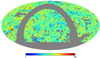 |
Fig. A.1. Source count map of the TGSS-ADR1 radio source catalogue with a flux density threshold of 100 mJy shown in equatorial coordinates and Mollweide projection, the cell size is given by Nside = 32. |
The corresponding differential source count is shown in Fig. 14 and compared to our results from LoTSS-DR1. Above 100 mJy both source counts agree very well. This also confirms the estimates of completeness in Intema et al. (2017). Figure 10 of that work shows a plot of the completeness of the TGSS-ADR1 source catalogue which we read off to be 95% at a flux density threshold of 100 mJy. This completeness estimate is based on the detection fraction, which is the fraction of TGSS source counts and SKADS source counts and the completeness is stated to be 50% at 25 mJy.
We also compare our results for the angular two-point correlation function for the LoTSS-DR1 2 mJy “mask 1” sample (see Sect. 6) to the masked TGSS-ADR1 at flux density thresholds of Smin = 100 and 200 mJy (see Fig. A.2). We made use of the error estimations computed by TREECORR using the same settings as in Sect. 6. The different flux density thresholds give self-consistent results and show stronger angular correlations than found from LoTSS-DR1. For separations between one and 10 degrees, the results of LoTSS and TGSS differ significantly. Additionally, we fitted with a power-law model w(θ) = A(θ/1 deg)−γ in linear space in the range 0.2 deg ≤θ ≤ 2 deg using LMFIT. The results of the fit are included in Table 6. We find somewhat larger angular correlations compared to the results in Rana & Bagla (2019), which is probably due to the fact that we include cells with averaged rms noise of up to 5 mJy beam−1, whereas Rana & Bagla (2019) exclude all cells in Nside = 1024 resolution that exceed averaged rms noise of 4 mJy beam−1. Thus we keep more radio sources for the analysis, as can be seen in Table 6. Another approach to estimate the angular two point correlation function of the TGSS-ADR1 catalogue was presented by Dolfi et al. (2019). They fitted a power law to small angular seperations θ ≤ 0.1 deg only and thus no quantitative comparison is shown here. To produce a reference catalogue of the TGSS, they masked regions and sources with greater rms noise than 5 mJ beam−1, declination < − 45 deg and Galactic latitude |b|< 10 deg in a resolution of Nside = 512 and included sources with flux density S ∈ [200, 1000] mJy. They find a smaller amplitude A = (6.5 ± 0.6) × 10−5, but much steeper slope γ = 2.87 ± 0.02 at θ < 0.1 deg. At θ > 0.1 deg, they also find a much flatter slope and see an excess of correlation with respect to the NVSS catalogue, but this result is just shown in a figure without quantifying the excess by a number.
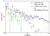 |
Fig. A.2. Comparison of the two-point correlation function w(θ) for the TGSS-ADR1 source catalogue for different flux density thresholds and for the LoTSS-DR1 value-added source catalogue. The errors shown are estimates by means of TREECORR and represent just statistical errors. We fitted w(θ) by a power-law in the range 0.2 deg ≤θ ≤ 2 deg. |
Appendix B: Comparison of different estimators for w(θ)
Several estimators have been suggested in the literature for the determination of the two-point correlation function. All those estimators are based on counting pairs per bin in angular separation θ and bin width Δθ. These pairs are denoted by
where Nd and Nr are the numbers of radio sources (data) and random (or mock) sources respectively.
We have written a brute force code to determine DD, DR, and RR exactly and to allow us to compare the performance of those estimators for the particular LoTSS-DR1 survey geometry and to test the accuracy of the software package TREECORR (see Appendix C). As a brute force computation of the two-point correlation function is numerically expensive (the estimation of the two-point correlation scales with  and the estimation of its variance scales with
  ), we restricted this tests to the S > 4 mJy sample of the LoTSS-DR1 value-added source catalogue with “mask d”, which had Nd = 30 556 and we used Nr = 20Nd sources from a purely random sample. We also investigated how the performance of different estimators scales for smaller random samples.
Figure B.1 shows the results for the following estimators:

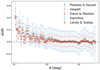 |
Fig. B.1. Comparison of five different estimators of the angular two-point correlation function w(θ). We evaluate it for the LoTSS-DR1 value-added source catalogue with S > 4 mJy after applying “mask d”. Here we compare to a truly random catalogue with Nr = 20Nd, rather than to the mock catalogue of Sect. 4. The errors are obtained via the variances from Table B.1. |
For most data bins, we find that  .
.
The expected biases and variances of the five estimators are tabulated in Table B.1. The results are expressed in terms of the quantities
Bias and variance of the five considered estimators of the angular two-point correlation function for the case Nr ≫ Nd and assuming |w(θ)| and |wΩ| (see Eq. (28)) are both small compared to unity.
where Gp is the fraction of pixel pairs separated by a given angular separation for pixels small enough such that they contain at most a single source. The fraction of triplets, Gt, is given as one source at the centre and two other at a given angular separation, respectively.
Between 2 and 8 degrees, all estimators give very similar results, cf. Fig. B.1. However, for separations larger than 10 degrees, the PH estimator shows a significant deviation compared to the results obtained with the Landy & Szalay estimator and with the Hamilton Estimator. The shown errors are underestimates since they are obtained via the variances from Table B.1. Hence, we assume that Nr ≫ Nd and |w(θ)| and |wΩ| (see Eq. (28)) are both small compared to unity.
Figure B.2 shows this expected variance for the different estimators. Since Gp is equivalent to RR, the random pair counts resulting from the use of the random catalogue with 620 440 points can be used to estimate Gp. However, the estimation of Gt scales with  . Due to the necessary computing time, Gt is estimated via 12 runs with 3 000 points each. It can be seen that the contribution of t to the variance is significant at all angular scales and dominates over the contribution of p.
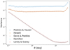 |
Fig. B.2. Estimated variance of different estimators for the LoTSS-DR1 value-added source catalogue at S > 4 mJy. The Landy & Szalay and Hamilton estimators have identical variance as well as the estimators by Hewett and Davis & Peebles. |
Our findings confirm previous studies of the performance of different estimators (Pons-Bordería et al. 1999; Kerscher et al. 2000; Vargas-Magaña et al. 2013), including the estimators studied in this work. These previous studies showed that the LS estimator operates best in almost every application, especially for wide separation ranges extending to the large scales, a typical feature of current surveys. However, the previous studies had their focus on the study of the three dimensional two-point correlation and investigated them in the context of galaxy redshift surveys rather than in the context of radio continuum surveys.
We also investigated how the results for the Landy and Szalay estimator depend on the sample size of the random catalogues. As can be seen in Fig. B.3, there is more fluctuation if small random samples are used. Especially at angular separations above 1 deg, Nr = 5Nd does already give rise to reliable estimates. Therefore, it would be a computational advantage to calculate the two-point correlation function with small random catalogues (but Nr > Nd) if only large separations are of interest.
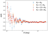 |
Fig. B.3. Comparison of the results for the two-point correlation function using the LS estimator and various sizes of random catalogues. For separations larger than 1 degree smaller random catalogues give results very similar to those from large random catalogues with Nr = 20Nd. The errors are estimated from Table B.1. |
Appendix C: Testing of the TreeCorr software package
The TREECORR software package (version 3.3) provides various parameters for setting options that enhance the accuracy of its computations. By default, TREECORR uses metric distances which are only accurate for small separations but are fast to calculate. In this work we also examine the two-point correlation function for larger separations up to 32 degrees. Therefore, great-circle distances are used to obtain accurate distance measurements on larger scales. TREECORR takes this option via metric = “Arc”, which is used throughout the following analysis.
Furthermore, the accuracy of the algorithm depends on the configuration parameter bin_slop. This parameter controls the accuracy of TREECORR to put pairs in the correct angular bin when identifying the many “trees”. For the chosen bin width of Δln(θ/1 deg) = 0.1, the default value is one. If this parameter is set to zero, as we do for the analysis presented in Sect. 6, TREECORR should give the most accurate result (more information can be found in the TREECORR-documentation8). Figure C.1 shows the values for the two-point correlation function when calculated from an exact brute force code (documented in Biermann 2019), calculated with TREECORR’s default value for bin_slop and using the best possible TREECORR precision bin_slop=0. By eye, the most precise TREECORR results are indistinguishable from the exact values. In contrast, the default settings give results that lead to misestimates that are of the order of the expected signal at angular scales of 1 deg. It is clear that the accuracy of the estimates should be at least an order of magnitude better than the expected signal. The analysis of NVSS (Condon et al. 1998) data suggests, that it should be at the level of 10−3 to 10−4 at angular scales above 1 deg (Blake & Wall 2002; Overzier et al. 2003). Hence, it is essential to modify the default settings of TREECORR to calculate accurate results.
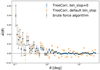 |
Fig. C.1. Test of the accuracy of TREECORR. We compare the TREECORR default settings (orange crosses) and the best possible TREECORR precision (bin_slop = 0) to the results from an exact brute force code (black dots). |
Using a smaller value for bin_slop extends the computing time, obviously. Using the default accuracy yields a computing time of a few seconds9, when using the 4 mJy flux density threshold and a random catalogue containing Nr = 20Nd points, whereas using the brute force setting (bin_slop=0) takes about 70 minutes. However, obtaining the most accurate results possible with TREECORR is still roughly 12 times faster than using our own brute force algorithm that we used for the purpose to check the performance of TREECORR.
Nonetheless, it is relevant to test other settings for TREECORR’s accuracy since, using lower flux density thresholds results in a higher number of sources and larger mock catalogues as mentioned in Sects. 5 and 6. Hence, the computational time increases significantly. We note also that a brute force estimate of the variance of  scales as
  , which poses substantial computational challenges for small flux density thresholds in upcoming data releases (we expect to lower our flux density threshold below 1 mJy for a cosmology analyis of LoTSS-DR2). Figure C.2 shows the absolute error of TREECORR results, with respect to the brute force algorithm and using values for the bin_slop of 1, 0.1, 0.05, and 0. Setting the value of bin_slop to 0.05 is roughly nine times faster and using a value of 0.1 is ∼24 faster than using the most exact settings. Brute force settings for TREECORR yield an absolute error of about 3.5 × 10⁻⁵ as it is almost constant over the considered separations. The origin of this constant offset is not further examined. It could be either caused by limitations of TREECORR or of the brute force algorithm or of both algorithms. A small value for the bin_slop can give more precise results in some cases, meaning that for some separations, however, the absolute error shows clear fluctuations. Using bin_slop=0.1 could result in absolute errors as high as the correlation function at separations of 3 deg and larger. Additionally, we show the relative error of TREECORR with respect to the brute force algorithm in Fig. C.2. The relative error is calculated via:
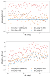 |
Fig. C.2. Top: mean absolute error of TREECORR with respect to the brute force algorithm. We compare the TREECORR default settings (red boxes), two small values for bin_slop (brown triangles: 0.1, orange diamonds: 0.05) and the best possible TREECORR precision (bin_slop = 0, blue circles). Bottom: relative error of TREECORR with respect to the brute force algorithm, calculated via Eq. (C.1). |
In order to test the error computation by TREECORR, we additionally estimate the error in our measurement of w(θ) for each bin via bootstrap re-sampling method as described by Ling et al. (1986). For this we use 100 pseudo-random samples of the same size as the original catalogue, generated by randomly choosing sources with replacement from the original catalogue. We then compute the angular two-point correlation function ( ) for each sub-sample and the bootstrap errors as the standard deviation given by the following equation.,
where w0(θ) is the mean value for the sub-samples and N the total count. Both error estimations for the LoTSS-DR1 value-added catalogue, masked with “mask d” and flux density thresholds of 1, 2, and 4 mJy are shown in Fig. C.3. The error estimate by TREECORR using bin_slop= 0 and bootstrapping agree within all three flux density thresholds and the difference between both is in maximum of order 4 × 10⁻⁴ in the range 0.1 ≤ θ ≤ 2 deg and of order 10−5 for larger separations. Therefore we decide to use error estimates done by TREECORR with bin_slop= 0 in our analysis.
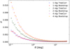 |
Fig. C.3. Comparison of errors calculated by TREECORR using bin_slop = 0 and by means of 100 bootstraps for the LoTSS-DR1 value-added catalogue after masking with “mask d”. |
The above findings are valid when using LoTSS-DR1 data and may vary for different surveys.
Appendix D: Kinematic radio dipole
Following Ellis & Baldwin (1984), the kinematic radio dipole, which is due to the proper motion of the Solar system, contributes to the source counts per solid angle with a Doppler shift of the emitted radiation from a source and the aberration of the observed source positions:
![$$ \begin{aligned} {\left( {\frac{{{\rm{dN}}}}{{{\rm{d}}\Omega }}} \right)_{{\rm{obs}}}} = {\left( {\frac{{{\rm{dN}}}}{{{\rm{d}}\Omega }}} \right)_{{\rm{rest}}}}\left[ {1 + [2 + x(1 + \alpha )]\beta {\rm{cos}}\theta } \right], \end{aligned} $$](/articles/aa/full_html/2020/11/aa36592-19/aa36592-19-eq104.gif)
with β = v⊙c−1 and x defined as:

The amplitude of the kinematic dipole is given by
![$$ \begin{aligned} d=[2+x(1+\alpha )]\beta , \end{aligned} $$](/articles/aa/full_html/2020/11/aa36592-19/aa36592-19-eq106.gif)
and θ measures the angle between the position of a source and the direction of Sun’s proper motion.
To estimate the contribution of the kinematic radio dipole to the angular two-point correlation function, we follow the procedure of Rubart & Schwarz (2013) and first generate a sky of random sources with associated random flux densities. The spherical coordinate positions (Φ, Θ) of simulated sources are drawn randomly by:


Using this definition, we already fulfil the convention of Co-Latitude necessary for HEALPIX. Additionally, we generate random flux densities:

We fix S0 = 0.9 mJy, such that we can apply a flux density threshold after boosting of 1 mJy.
We then calculate boost and aberration for each individual source, where we use the latest findings of Planck (Planck Collaboration I 2020). They infer the proper motion of the Sun to be v⊙ = 369.82 ± 0.11 km s−1 towards (167.942 ± 0.011, − 6.944 ± 0.005) deg in Equatorial coordinates (J2000), which results in a kinematic radio dipole amplitude of:
where we assumed typical values of x = 1 and α = 0.75 for the boosting.
From this boosted simulation, we estimate the angular two-point correlation using the same settings as described in Sect. 2.3, where the total number of simulated sources is fixed to the amount of sources in the LoTSS-DR1 “Any z” sample, together with a pure random sample. The results of this estimation is compared in Fig. D.1 to the LoTSS-DR1 “Any z" sample with a 1 mJy flux density threshold. We see an order of magnitude lower correlation than observed in the actual data sample and therefore neglect the dipole term in our theoretical expectation.
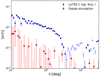 |
Fig. D.1. Comparison of the two-point correlation function w(θ) for the 1 mJy “Any z” sample of the LoTSS-DR1 value added source catalogue and a simulated sky with contribution from a kinematic dipole. Negative values are shown with open symbols. |
All Tables
Number of included cells (Ncell) and sky coverage (Ω) for different masks and flux density thresholds (Smin).
Pearson χ2-test statistic of counts-in-cell distribution for the masked LoTSS-DR1 value-added source catalogue with “mask d” for four flux density thresholds.
Number of sources of the masked (mask z) LoTSS-DR1 value-added source catalogue for various flux density thresholds and for different values of minimum redshift z.
Best-fit values of w(θ) = A(θ/1 deg)−γ, fitted in the range 0.2 ≤ θ ≤ 2.0 deg and corresponding integral constraint wΩ for the LoTSS-DR1 value-added source catalogue after appropriate masking and for the TGSS-ADR1 catalogue, with 68% confidence intervals.
Bias and variance of the five considered estimators of the angular two-point correlation function for the case Nr ≫ Nd and assuming |w(θ)| and |wΩ| (see Eq. (28)) are both small compared to unity.
All Figures
|
Fig. 1. Distribution of radio sources observed in the LoTSS-DR1 HETDEX spring field. Plotted are all individual sources (top), as well as the number counts per cell in Cartesian projection at HEALPIX resolution Nside = 256 (bottom). Observed are nearly 325 000 sources within 58 pointings on the sky covering 424 square degrees. The positions of the five brightest radio sources in terms of integrated flux density are indicated in black (see Sect. 3.3 for details). |
| In the text | |
|
Fig. 2. Left: estimated point-source completeness for each of the 58 pointings in the HETDEX field as a function of flux density. Blue, green and red (dotted) lines indicate inner, outer and the five most incomplete pointings, respectively. Right: mean point source completeness of all pointings (solid line) and after rejection of the five most incomplete pointings (dotted line). |
| In the text | |
|
Fig. 3. Top: completeness of the LoTSS-DR1 catalogue per HEALPIX cell. Bottom: completeness of cells after applying a flux density threshold of 0.39 mJy, which corresponds to an overall point source completeness of 95%. |
| In the text | |
|
Fig. 4. Top: source counts for each pointing within angular distance θ around the pointing centre, normalised by covered area. Pointings are classified by position in the HETDEX field, with pointings on the edge (green), in the inner field (blue) and undersampled ones (red, dotted). The mean is shown in black with standard deviation (grey band) of all pointings. Bottom: source counts around the five brightest radio sources in terms of integrated flux density from the radio source (dashed lines) and value-added source catalogue (solid lines). The mean number counts around the five brightest sources are shown in black for both catalogues and additionally also the mean over all pointings (dash dotted). |
| In the text | |
|
Fig. 5. LoTSS-DR1 HETDEX spring field masks: “mask p” rejects all cells shown in dark blue and includes 53 pointings modelled by discs of radius 1.7 deg. Our default “mask d” additionally rejects cells with less than five sources (yellow cells), see also text in Sect. 3.4. For analysis that includes redshift information “mask z” additionally rejects a strip shown in light blue. For further details, see the text in Sect. 5.3. |
| In the text | |
|
Fig. 6. Histogram of source counts per cell (blue) and binned Poisson distribution with empirical mean (red line) from the LoTSS-DR1 radio source catalogue at Nside = 256, masked and including only cells with at least five sources (mask d). |
| In the text | |
|
Fig. 7. Local rms noise per HEALPIX cell, calculated via the mean of the local rms around each LoTSS-DR1 radio source. The heat map (top) and histogram (bottom) of the local rms is clipped at an upper limit of five times the median rms noise. The median rms noise of 0.07 mJy beam−1, as well as the values of two and three times the median rms noise are marked in the histogram with black dashed lines. |
| In the text | |
|
Fig. 8. Sky coverage of the three local rms noise masks. The red cells are included for an average noise < 0.07 mJy beam−1 in the HEALPIX cells (“mask 1”), red and yellow pixels are included for an average noise of < 0.14 mJy beam−1 (“mask 2”) and red, yellow and light blue cells are included for an average noise of < 0.21 mJy beam−1 (“mask 3”). Dark blue cells are additionally included in “mask d”. Regions in grey are excluded by all masks. |
| In the text | |
|
Fig. 9. Mock catalogue of random sources that are detectable at five times the local rms noise and masked with “mask d”. |
| In the text | |
|
Fig. 10. Sample statistics of number counts in cells as a function of flux density threshold. Shown are the clustering parameter nc (variance over mean), which is expected to be one for the Poisson distribution, the skewness g1 and excess kurtosis g2 − 3 with error bars calculated from 100 bootstrap samples. On the left hand side for the LoTSS-DR1 radio source catalogue, on the right hand side for the LoTSS-DR1 value-added source catalogue. From top to bottom: mask d and masks 2 and 1. |
| In the text | |
|
Fig. 11. Skewness (g1) and excess kurtosis (g2 − 3) of the masked LoTSS DR1 value-added source catalogue (mask d), also plotted are the expected moments of a Poisson and compound Poisson distribution. Errors bars for the data sample are computed from bootstrap sampling. |
| In the text | |
|
Fig. 12. Histograms of LoTSS-DR1 counts-in-cell for the flux density thresholds 1, 2, 4 and 8 mJy. Also shown are the best-fit Poisson and compound Poisson distributions. |
| In the text | |
|
Fig. 13. Clustering parameter and coefficients of skewness and kurtosis for a sub-sample of the mock catalogue, which matches the size of the value-added source catalogue. Error bars are computed from bootstrap sampling. |
| In the text | |
|
Fig. 14. Differential number counts per flux density interval of the masked LoTSS-DR1 value-added source catalogue for four different masks. Additionally the masked TGSS-ADR1 (147.5 MHz; this work, blue circle), the LOFAR Boötes field (Williams et al. 2016, orange triangle) and the MWA (154 MHz; Franzen et al. 2016, green box) are shown. Error bars for the LoTSS and TGSS counts are due to Poisson noise in each flux density bin, which have equal step width in log10(S). |
| In the text | |
|
Fig. 15. Top: comparison of LoTSS-DR1 differential source counts using “mask d” and SKADS 151 MHz and T-RECS “wide” 150 MHz simulations. The grey band corresponds to a ±20% variation of the LoTSS flux density scale due to uncertainties in the flux density calibration. Bottom: contributions from AGNs and SFGs in the T-RECS “wide” differential source counts as compared to the total LoTSS-DR1 differential source counts. All: error bars are due to Poisson noise in each flux density bin, which have equal bin width in log10(S). |
| In the text | |
|
Fig. 16. Number of radio sources as a function of available z for four different flux density thresholds, with error bars due to Poisson noise. Only sources with available redshift (“z_best”) of the LoTSS-DR1 value added source catalogue after applying “mask z” are considered here. |
| In the text | |
|
Fig. 17. Differential source counts of the LoTSS-DR1 value-added sources masked with “mask z” separated by redshift percentiles, z33 = 0.376 and z66 = 0.705. Additionally the differential source counts of all sources (“All”) and of all sources with redshift information (“Any z”) are shown. |
| In the text | |
|
Fig. 18. Clustering parameter nc as function of flux density threshold and available redshift information based on the value “z_best” from the LoTSS-DR1 value-added source catalogue after application of “mask z”. Top: we compare radio sources with and without redshift information and contrast them with the full sample. Bottom: only objects with redshifts above the quoted value are included in the respective data points. Error bars are computed from bootstrap sampling. |
| In the text | |
|
Fig. 19. Counts-in-cell map of the LoTSS-DR1 value-added source catalogue for S > 1.0 mJy and after applying “mask d” (left) and “mask 1” (right). |
| In the text | |
|
Fig. 20. Angular two-point correlation of sources from the LoTSS-DR1 value-added source catalogue after masking with “mask d” (top) and “mask 1” (bottom) and at flux densities above 1, 2, and 4 mJy. Positive and negative values are shown with full and open symbols, respectively. The grey shaded region indicates angular separations with decreasing number of weighted pair counts. |
| In the text | |
|
Fig. 21. Comparison of two-point angular (auto-)correlation functions for “mask d” for different random catalogues: mock catalogue based on LoTSS local rms noise (data-mock), homogeneous random catalogue accounting for survey geometry only (data-random), and the correlation of the mock catalogue (mock-random) for flux densities above 1 mJy (top) and 2 mJy (bottom). We fitted the data to the power-law model described in the text. Positive and negative values are shown with full and open symbols, respectively. The grey shaded region indicates angular separations with decreasing number of weighted pair counts. |
| In the text | |
|
Fig. 22. Angular two-point correlation from the LoTSS-DR1 value-added source catalogue after masking with “mask d”, “mask 1”, and “mask 2” at flux densities above 1 mJy (top) and 2 mJy (bottom) for data-mock pairs; see caption of Fig. 21 for further details. We fitted the data of “mask 1” to the power-law model described in the text. Positive and negative values are shown with full and open symbols, respectively. The grey shaded region indicates angular separations with decreasing number of weighted pair counts. |
| In the text | |
|
Fig. 23. Angular two-point correlation function of sources from the LoTSS-DR1 value-added source catalogue with “mask d” and flux density threshold of 1 mJy and 2 mJy, for three regions namely “Left”, “Center”, and “Right”. |
| In the text | |
|
Fig. 24. Angular two-point correlation function of sources from the LoTSS-DR1 value-added source catalogue with “mask 1” and flux density threshold of 1 mJy and 2 mJy, for three regions namely “Left”, “Center”, and “Right”. |
| In the text | |
|
Fig. 25. Comparison of the angular two-point correlation function estimated from the LoTSS-DR1 value-added source catalogue for radio sources with redshift information and theoretical expectations (solid lines) for the best-fit ΛCDM cosmological parameters from Planck, generated using CAMB SOURCES with Halofit and b(z) from Eq. (28). The integral constraint wΩ is computed for the expectations and subtracted from them. Positive values are shown with full symbols and solid lines, whereas negative values are shown with open symbols and dashed lines. |
| In the text | |
|
Fig. 26. Angular two-point correlation function for three redshift bins z1, z2 and z3 for a flux density threshold of 2 mJy. The lines show the expectations for the cosmological standard model. Both panels use the Halofit option of CAMB SOURCES, which accounts for the non-linear evolution of large scale structure. In the top panel we use the bias function of Eq. (32), whereas we use a piecewise constant bias in the bottom panel. The integral constraint wΩ is computed for the expectations and subtracted from them. Positive values are shown with full symbols and solid lines, whereas negative values are shown with open symbols and dashed lines. |
| In the text | |
|
Fig. A.1. Source count map of the TGSS-ADR1 radio source catalogue with a flux density threshold of 100 mJy shown in equatorial coordinates and Mollweide projection, the cell size is given by Nside = 32. |
| In the text | |
|
Fig. A.2. Comparison of the two-point correlation function w(θ) for the TGSS-ADR1 source catalogue for different flux density thresholds and for the LoTSS-DR1 value-added source catalogue. The errors shown are estimates by means of TREECORR and represent just statistical errors. We fitted w(θ) by a power-law in the range 0.2 deg ≤θ ≤ 2 deg. |
| In the text | |
|
Fig. B.1. Comparison of five different estimators of the angular two-point correlation function w(θ). We evaluate it for the LoTSS-DR1 value-added source catalogue with S > 4 mJy after applying “mask d”. Here we compare to a truly random catalogue with Nr = 20Nd, rather than to the mock catalogue of Sect. 4. The errors are obtained via the variances from Table B.1. |
| In the text | |
|
Fig. B.2. Estimated variance of different estimators for the LoTSS-DR1 value-added source catalogue at S > 4 mJy. The Landy & Szalay and Hamilton estimators have identical variance as well as the estimators by Hewett and Davis & Peebles. |
| In the text | |
|
Fig. B.3. Comparison of the results for the two-point correlation function using the LS estimator and various sizes of random catalogues. For separations larger than 1 degree smaller random catalogues give results very similar to those from large random catalogues with Nr = 20Nd. The errors are estimated from Table B.1. |
| In the text | |
|
Fig. C.1. Test of the accuracy of TREECORR. We compare the TREECORR default settings (orange crosses) and the best possible TREECORR precision (bin_slop = 0) to the results from an exact brute force code (black dots). |
| In the text | |
|
Fig. C.2. Top: mean absolute error of TREECORR with respect to the brute force algorithm. We compare the TREECORR default settings (red boxes), two small values for bin_slop (brown triangles: 0.1, orange diamonds: 0.05) and the best possible TREECORR precision (bin_slop = 0, blue circles). Bottom: relative error of TREECORR with respect to the brute force algorithm, calculated via Eq. (C.1). |
| In the text | |
|
Fig. C.3. Comparison of errors calculated by TREECORR using bin_slop = 0 and by means of 100 bootstraps for the LoTSS-DR1 value-added catalogue after masking with “mask d”. |
| In the text | |
|
Fig. D.1. Comparison of the two-point correlation function w(θ) for the 1 mJy “Any z” sample of the LoTSS-DR1 value added source catalogue and a simulated sky with contribution from a kinematic dipole. Negative values are shown with open symbols. |
| In the text | |
Current usage metrics show cumulative count of Article Views (full-text article views including HTML views, PDF and ePub downloads, according to the available data) and Abstracts Views on Vision4Press platform.
Data correspond to usage on the plateform after 2015. The current usage metrics is available 48-96 hours after online publication and is updated daily on week days.
Initial download of the metrics may take a while.