| Issue |
A&A
Volume 642, October 2020
|
|
|---|---|---|
| Article Number | A94 | |
| Number of page(s) | 8 | |
| Section | Extragalactic astronomy | |
| DOI | https://doi.org/10.1051/0004-6361/202038684 | |
| Published online | 08 October 2020 | |
An extreme ultraluminous X-ray source X-1 in NGC 5055
Nicolaus Copernicus Astronomical Center, Polish Academy of Sciences, ul. Bartycka 18, 00-716 Warsaw, Poland
e-mail: smondal@camk.edu.pl
Received:
17
June
2020
Accepted:
4
August
2020
Aims. We analysed multi-epoch X-ray data of the ultraluminous X-ray source NGC 5055 X-1, with luminosity up to 2.32 × 1040 erg s−1, to constrain the physical parameters of the source.
Methods. We performed a timing and spectral analysis of Chandra and XMM-Newton observations. We used spectral models that assume the emission is from an accreting black hole system. We fit the data with a multicolour disk combined with a powerlaw or a thermal Comptonization (NTHCOMP) component and compared those fits with a slim disk model.
Results. The light curves of the source do not show significant variability. From the hardness ratios (3–10 keV/0.3–3 keV flux), we infer that the source is not spectrally variable. We found that the photon index is tightly, positively correlated with the unabsorbed 0.3–10 keV flux and the hydrogen column density. Furthermore, the temperature emissivity profile indicates a deviation from the standard sub-Eddington thin disk model. The source shows an inverse correlation between luminosity and inner disk temperature in all fitted models.
Conclusions. Our analysis favours the source to be in an ultraluminous soft state. The positive correlations between the photon index and the flux as well as between the photon index and the hydrogen column density may suggest the source is accreting at high Eddington ratios and might indicate the presence of a wind. The inverse luminosity relation with the inner disk temperature for all spectral models may indicate that the emission is geometrically beamed by an optically thick outflow.
Key words: accretion / accretion disks / X-rays: individuals: NGC5055 X-1 / stars: black holes
© ESO 2020
1. Introduction
Ultraluminous X-ray sources (ULXs) are off-nuclear point sources with isotropic X-ray luminosity in excess of 1039 erg s−1 (Fabbiano 1989). Due to their high luminosity, it had been suggested in the past that ULXs may be host to an intermediate mass black hole (IMBH, Colbert & Mushotzky 1999); however, the recent discovery of coherent pulsations have indicated that some ULXs contain a neutron star (Bachetti et al. 2014; Fürst et al. 2016, 2017; Israel et al. 2017a,b; Carpano et al. 2018). This finding was independently confirmed in three sources through a fitting with a spectral model that assumes non-isotropic emission from a neutron star-accretion disk system (Różańska et al. 2018). These ULXs are also exciting in the context of gravitational wave studies. Some ULXs have a high-mass donor (Motch et al. 2011, 2014; Heida et al. 2015, 2016) that might eventually form the merging of two compact objects at the end of its stellar evolution (Mondal et al. 2020).
As most ULXs are extra-galactic sources, the direct measurement of the mass of the compact object is extremely difficult. Therefore, we have to rely on indirect methods, such as BH mass-scaling of the inner disk temperature (Tin ∝ M−1/4) (Miller et al. 2003). Most ULX spectra are fitted with a two-component model: a multicolor accretion disk model (MCD) and a hard powerlaw (PL) tail. Fitting this model to a number of ULX spectra results in a very cool inner disk temperature, kTin ∼ 0.1 − 0.3 keV and a PL tail Γ ∼ 1.5 − 3 (Kaaret et al. 2003; Miller et al. 2004a,b). If this temperature corresponds to the temperature at the inner disk radius, then the inferred BH mass would be ∼103 M⊙. This supports the IMBH interpretation with a sub-Eddington accretion rate, although ULXs spectra do not clearly resemble the typical low-hard or high-soft state spectra of BH X-ray binaries (BHXBs). However, studies of Galactic BHXBs have shown that the derived temperature from the disk component is reliable only when the spectrum is dominated by the disk emission (Done & Kubota 2006). As the contribution from the PL tail component becomes significant, the derived disk temperature is extremely unreliable.
Observations have shown ULXs to exhibit various types of spectral shapes. High-quality XMM-Newton data revealed spectral curvature associated with the hard X-ray emission component in the 2–10 keV band (Stobbart et al. 2006; Gladstone et al. 2009; Kajava et al. 2012). Fits with phenomenological spectral models allowed for the identification of four main types of spectral shapes: soft ultraluminous, hard ultraluminous, broadened disk, and super soft ultraluminous. These four types have been ascribed to different accretion regimes (Kaaret et al. 2017).
King et al. (2001) suggested that most ULXs have a stellar mass compact object accreting at a super-Eddington rate and their high luminosity results from the beaming of the X-ray emission due to a geometrically thick wind outflowing from the disk. In fitting of some ULX spectra with MCD plus PL components, Feng & Kaaret (2007) and Kajava & Poutanen (2009) found that the temperature of the soft component is inversely correlated with luminosity L ∝ T−3.5, which is at odds with the L ∝ T4 relation expected from theory and observed in BHXBs (Gierliński & Done 2004). King & Puchnarewicz (2002) showed that this inverse relation is actually expected when the source is beamed and accreting at a super-Eddington rate. Motivated by the observed soft temperature-luminosity relation King (2009) derived an empirical relation describing the scaling of the beaming factor with the inverse of the square of the accretion rate, which implies that the most luminous ULXs are highly collimated. However, in the presence of a powerful disk wind one would expect that at large distances from the BH the wind becomes optically thin, and emission or absorption lines associated with radiation passing through the partially ionized optically thin phase of the wind can be observed. Such features have been found in recent studies of NGC 5408 X-1 and NGC 6946 X-1 by Middleton et al. (2014) and of NGC 1313 X-1 and NGC 5408 X-1 by Pinto et al. (2016).
Here, we report on the analysis of Chandra and XMM-Newton observations of an extreme ULX in the outskirts of the spiral galaxy NGC 5055 (M63). The source NGC 5055 X-1, was serendipitously discovered by ROSAT High Resolution Imager (HRI; Roberts & Warwick 2000). Follow-up observations were carried out by Chandra, XMM-Newton and Swift. In spite of its being very luminous in the X-ray band, reaching ∼ 2.3 × 1040 erg s−1 (Swartz et al. 2011), the source has received very little attention and none of the available X-ray observations are reported in the literature.
In this paper, we perform the first systematic analysis of X-ray observations of NGC 5055 X-1, using three longest Chandra and XMM observations. We carried out X-ray timing and spectral analysis, using phenomenological models available in XSPEC fitting package (Arnaud et al. 1996). The data reduction process is presented in Sect. 2. The timing and spectral analysis are presented in Sects. 3 and 4. The most important correlations among the physical parameters are shown in Sect. 5 and the conclusions are reported in Sect. 6.
2. Observations and data reduction
The source NGC5055 X-1 is located at RA = 13h15m19.54s and Dec = 42°03′02.3″. The distance to the galaxy has been reported to be 9.2 Mpc (Tully et al. 2013; Tikhonov et al. 2015; McQuinn et al. 2017) and we use this value throughout this paper. There are many observations of NGC 5055 X-1 by several X-ray observatories, but most of them are short observations with insufficient counts to allow for a meaningful spectral analysis. Most of the Swift observations have an exposure time of ≲10.0 ks and total counts ∼160. The only three long observations available are from Chandra ACIS-S and XMM-Newton EPIC-MOS1, MOS2, and EPIC-PN, with a total of ∼1000 net counts, which we used in this study. The details of these observations are given in Table 1.
Details of X-ray observations analysed in this paper.
For the data reduction, standard procedures were followed, as described in detail in the following subsections. In all cases, NGC5055 X-1 was located in the field of view, but close to the edge of the chip, as shown in Fig. 1, where the X-ray images of the source from both satellites are presented.
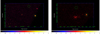 |
Fig. 1. X-ray image in counts per pixel displays the field of view of Chandra ACIS-S (left panel) and XMM-Newton EPIC-MOS1 (2007-05-28; right panel) detectors. The green circles containing bright pixels show NGC 5055 X-1, while the empty green circles represent the region from where the background was extracted. Chandra spatial resolution allowed us to extract source photons from a circular region of 6″ radius, while for XMM-Newton we used circular regions of 40″. |
2.1. Chandra data
We reduced the data from the ACIS-S detector using the standard pipeline Chandra Interactive Analysis software CIAOv4.12. NGC 5055 X-1 was detected close to the edge of the field of view (see left panel of Fig. 1), while the observatory pointed at the center of NGC 5055. We used chandra_repo to remove the hot pixels, creating new event files and producing good time intervals. The source and background were extracted from a circular region of 6″ radius as shown in Fig. 1 left (green circles). The background-subtracted source light curve was created using dmextract. The spectrum was generated using specextract, taking into account the correction for the point spread function (PSF) for off-axis sources. The auxiliary files and redistribution matrices were generated with specextract using the module mkarf and mkrmf, respectively. Given that NGC 5055 X-1 is close to the chip edge (see Fig. 1), the spacecraft dither may cause the temporal disappearance of the source from the field of view. We have taken this into account in our timing analysis (see Sect. 3) and when making auxiliary files for spectral analysis.
2.2. XMM-Newton
The data reduction was carried out using XMM-Newton Science Analysis System (SASv16.0.0) following standard procedures. The observation data files (ODF) were processed using emproc and epproc to create calibrated event lists for EPIC-MOS and EPIC-PN detectors, respectively. A circular region of 40″ radius was chosen to extract source and background counts. We used evselect to generate light curves and spectra selecting single and double events for the EPIC-PN detector and single to quadruple events for the EPIC-MOS detector. The source light curve was corrected from background counts using epiclccorr. The auxiliary files and redistribution matrices were generated using arfgen and rmfgen. We note that for the XMM-Newton observation in June 2007, the EPIC-MOS and EPIC-PN were not observing strictly simultaneously. There is a ∼52 min of delay between the start times of EPIC-MOS and EPIC-PN, which results in a shorter effective (after removing periods of flaring background) exposure time for EPIC-PN, as listed in Table 1.
3. Timing analysis
The main purpose of our timing analysis is to find out if the source shows significant temporal and spectral variability. We used Stingray1 (Huppenkothen et al. 2019) to construct power spectral density (PSD) from the extracted light curves. Stingray is an open source spectral-timing Python software package for astrophysical data analysis.
We used the XMM-Newton EPIC-PN light curves for timing analysis as the EPIC-PN detector has higher full frame time resolution (73.4 ms) and greater effective area than the EPIC-MOS cameras. The light curves were extracted with a time bin of 0.22 s (three times the temporal resolution) to have enough counts in each bin. We used a 9.6 s time bin (Chandra temporal resolution is 3.2 s) to extract the light curves from Chandra ACIS-S observation. Figure 2 shows the ACIS-S and EPIC-PN light curves for the two bands, 0.3–3 keV and 3–10 keV, re-binned with a bin size of 500 s. We do not show light curves from both MOS cameras in the figure due to their lower signal-to-noise (S/N). The source does not display either flux nor spectral variability.
 |
Fig. 2. Chandra ACIS-S and XMM-Newton EPIC-PN light curves of NGC 5055 X-1 for the three observations at different epochs (observation IDs are indicated in each panel). Soft 0.3–3 keV and hard 3–10 keV energy band light curves are shown in the upper and middle panels, respectively, while the bottom panels show the hardness ratios for each set of data. All the light curves are re-binned with bin size 500 s to have higher S/N. The zero times in the plots correspond to 2001-08-27 02:13:48, 2007-05-28 07:59:14, and 2007-06-19 10:56:29 for panels from left to right, respectively. |
Nonetheless, ACIS-S light curves show enhanced variability with an apparently quasi-periodic pattern. The hardness ratios are consistent with being constant (left most panel of Fig. 2). We constructed PSD from ACIS-S light curves to explore the nature of the periodic pattern. To this aim, we used the unrebinned light curves, with a time resolution of 9.6 s. Each individual light curve was divided into four segments and the PSD was computed in each segment separately. Then, we averaged the PSD from the four segments.
From the Chandra data, we found periodic variations corresponding to two peaks at 1.4 mHz and 2.8 mHz. Such features are clearly not observed during XMM observations. While the hypothesis of a quasi-periodic feature in Chandra light curves disappearing in later XMM observations is appealing, we verified that this is most likely an instrumental artifact. Indeed, as pointed out in Sect. 2.1, the satellite dithering motion combined with the position of the source near the edge chip, may cause the source to periodically disappear. To verify this, we used the CIAO tool glvary to search for significant variability in Chandra light curves. The glvary tool utilizes information from the dither_region tool to correct the instrumental effects. The dither_region tool calculates the fractional area of the source region as a function of time that takes into account the corrections for chip edges, bad pixels, and bad columns. As an output, glvary computes the probability that the light curve is variable using a Gregory-Loredo algorithm (Gregory & Loredo 1992). The resulting probability values for the 0.3–3 keV and 3–10 keV light curves are 0.02 and 0.07, respectively, which would indicate that the source is not significantly variable. In Fig. 3, the Chandra probability-weighted light curves obtained with glvary are presented. We conclude that the source is not significantly variable and the quasi-periodic feature is an instrumental artefact. A more detailed description on how the dither motion affects the observed light curves for sources located near the chip edge is given in Roberts et al. (2004).
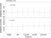 |
Fig. 3. Chandra observation probability-weighted light curves, as obtained from the CIAO glvary tool, i.e. after taking account all instrumental effects. The zero time corresponds to 2001-08-27 02:13:48. The total probability of variability for the 0.3–3 keV and 3–10 keV light curves is 0.02 and 0.07, respectively (see Sect. 3). |
4. Spectral analysis
As the hardness ratios presented in Figs. 2 and 3 (lowest panels) do not show significant indications of spectral variability, we carried out fits to the time-averaged spectra of the single observations. We tested simple accretion disk models in order to understand the basic properties of the source. We utilized the XSPECv12.10.1 (Arnaud et al. 1996) software for spectral analysis and different spectral models were used to fit the data: we first fit a simple MCD using the DISKBB model in XSPEC, then we added a POWERLAW component (MCD+PL); next we considered slim disk emission (DISKPBB model, Mineshige et al. 1994; Hirano et al. 1995; Watarai et al. 2000; Kubota & Makishima 2004; Kubota et al. 2005); and, finally, we considered a thermal Comptonization component due to a hot corona (MCD+NTHCOMP, Zdziarski et al. 1996; Życki et al. 1999). The spectra are fitted in the band of 0.3–10 keV and re-binned to have minimum of 20 counts in each energy bin. The effect of interstellar absorption was accounted for using TBNEW2. We let the hydrogen column density NH free to vary, keeping in mind that the value of Galactic absorption towards NGC 5055 is estimated to be ∼ 3.57 × 1020 cm−2 (HI4PI Collaboration 2016).
Following standard recommendations (see SAS website3), we did not co-add the spectra from each XMM-Newton detector, but we fit them simultaneously. We used the same models for Chandra and XMM-Newton data sets and, as a result, we obtained constraints on the physical parameters from three different epochs.
As a first step, we tested the well-known MCD model, representing emission from a standard Shakura & Sunyaev (1973) thin disk. The standard disk model is appropriate when the source accretion rate is below the Eddington value, assuming that the accretion disk is geometrically thin (h/r ≪ 1.0) and the radiation is emitted locally as black body from optically thick gas. When we fit each data set with a single MCD, the reduced χ2 is high and the ratio of data to the model significantly differs from unity as shown in Fig. 4. Furthermore, the best-fit NH value is very low, much lower than the estimated value for Galactic absorption, which suggests that the fit is unphysical.
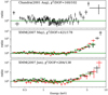 |
Fig. 4. Ratio of data to the folded model obtained from the fit of a MCD model, using DISKBB in XSPEC. The MCD model clearly leaves an excess at high energies. In XMM-Newton panels, the black, red, and green data points are, respectively, the spectra from EPIC-PN, EPIC-MOS1, and EPIC-MOS2. |
By adding an extra PL component to the MCD model, we obtained an excellent fit for all the three data sets, as described in Table 2 and shown in Fig. 5 (upper panels). The inner accretion disk temperature is relatively low compared to the values typically observed in Galactic BHXBs in the soft state (Gierliński & Done 2004). Assuming the source is in a state similar to the soft state, then the low temperature is consistent with an IMBH of ∼103 M⊙. The first XMM-Newton data set (2007-05-28) has higher flux than the second data set (2007-06-19), but slightly lower than in Chandra data. The required Galactic NH in Chandra is twice as large than in both XMM-Newton data sets.
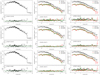 |
Fig. 5. Each subplot shows the data with the folded model in the upper panel and the data-to-model ratio in the lower panel. In the first row, results from the fit of the MCD+PL model are presented, in the second row the DISKPBB model, and, finally, in the third row we have MCD+NTHCOMP. The different columns correspond to Chandra data in the left column, XMM-Newton 2007-05-28 data in the middle column, and 2007-06-19 data in the right column. |
Best-fit parameters obtained from the fits of each set of data.
However, the assumption of a geometrically thin and optically thick disk is not valid when the source is close or above the Eddington limit. The luminosity of NGC 5055 X-1 is very high. If the accretor is a stellar mass BH, then the accretion rate is well above the Eddington rate. Assuming a 10 M⊙ BH and isotropic emission, we infer Ṁacc > 104 ṀEdd, and bolometric luminosity to be:
![$$ \begin{aligned} L_{\rm bol}=L_{\rm Edd}[1+\text{ ln}(\dot{M}_{\rm acc}/\dot{M}_{\rm Edd})]. \end{aligned} $$](/articles/aa/full_html/2020/10/aa38684-20/aa38684-20-eq32.gif)
In the regime of super-Eddington accretion, the disk becomes geometrically thick (h/r ∼ 1) and the photon diffusion timescale in the vertical direction becomes much longer than the radial in-fall timescale. This allows some of the photons to be advected radially into the BH, rather than emitted locally, which leads to a flatter effective temperature profile (Abramowicz et al. 1988; Watarai et al. 2000). The high luminosity of NGC 5055 X-1 suggests that the accretion rate may be extremely high. In this case, we would expect a substantially different temperature profile than in the standard thin disk model. The DISKPBB slim disk model allows the disk radial temperature profile to be fit to the data, with the local disk temperature, T(r) ∝ r−p, where p is a free parameter. The standard MCD model is recovered if p = 0.75 and this has been usually applied in previous studies of ULXs.
The DISKPBB model, while providing an overall acceptable description of the data, yields slightly worse fits, as shown in the middle row panels of Fig. 5. All best-fit parameters are described in Table 2. The Galactic NH is lower than in the case of MCD+PL model, giving a higher inner disk temperature, namely, kTin = 1.27, 1.98, and 2.86 keV for the first, second, and third data set, respectively. The temperature profile obtained from this model is the same in all data sets, that is, T(r) ∝ r−0.5, which is significantly different from that of the thin disk model (p = 0.75).
The fit with MCD+NTHCOMP model, presented in the bottom panels of Fig. 5, gives the same reduced χ2 and the same disk Tin as the MCD+PL model (see Table 2 for details). The only difference is the value of the Galactic absorption, which, in the case of the MCD+NTHCOMP model, has lower values than in other models, but is still in agreement with independent measurements of NH (as reported by HI4PI Collaboration 2016), for the first two data sets. This means that the normalization and, hence, the contribution of the MCD component is higher when fitted together with the NTHCOMP component than with a simple PL component, as illustrated in Fig. 6. Even if the fit statistic does not allow us to differentiate between those two models, the inferred value of Galactic absorption slightly favours the MCD+NTHCOMP model. The second reason to favour the model with thermal Comptonization is that in this model the two components are physically linked in a self-consistent way, that is, the temperature of the corona and, hence, the low energy cut-off of NTHCOMP depend on the inner disk temperature. On the contrary, the PL component does not have a low energy cut-off and, therefore, the model is less physical. The temperature of the corona from the MCD+NTHCOMP best-fit model is quite low kTe ∼ 1.68 − 1.78 keV. This is commonly observed in ULXs (Gladstone et al. 2009) and can be ascribed to a cool corona, reminiscent of the soft X-ray excess often observed in some BH accreting sources (Gronkiewicz & Różańska 2020; Petrucci et al. 2020, and references therein).
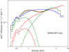 |
Fig. 6. Unfolded absorbed models (solid lines) and model components (dot-dashed line for MCD and dashed line for NTHCOMP and PL) fitted to the XMM-Newton 2007-06-19 data. Red lines represent the MCD+PL model, the blue line is the DISKPBB model, and green lines show the MCD+NTHCOMP model in which the MCD component is the most prominent. |
All the applied models give an unabsorbed X-ray flux in the 0.3-10 keV band, within the range 1.0 − 2.3 × 10⁻¹² erg s−1 cm−2, as reported in Table 2. Considering a distance of 9.2 Mpc to NGC 5055, these results correspond to an isotropic luminosity in the range 1.1 − 2.3 × 1040 erg s−1, as listed in Table 2. Sources in the luminosity range of 1040 − 1041 erg s−1 are classified as extremely luminous X-ray sources (ELX; Devi et al. 2007; Singha & Devi 2019). An ELX resembles the so called ultraluminous (UL) spectral state (Sutton et al. 2013). These UL hard states (dominated by emission from a hot corona) and UL soft states (dominated by emission from a cool corona) have been observed (Gladstone et al. 2009). Based on the data of NGC 5055 X-1, it is not possible to clearly discern whether the source might be in a UL hard state, which is characterized by a hard powerlaw, or in a UL soft state, in which the power law shows a cut-off at lower energies. Given the inferred best-fit electron temperatures, the slightly more favourable MCD+NTHCOMP model suggests that the source is in a UL soft state.
To illustrate this issue, in Fig. 6 we plotted the unfolded models for one XMM-Newton observation (2007-06-19). From a statistical point of view, those models do not differ significantly, but our previous considerations regarding the NH favour the MCD+NTHCOMP model. Longer observations extending to hard X-ray energies (e.g. by NuSTAR) are needed to better resolve the high energy tail and confirm this interpretation.
5. Discussion
Our spectral analysis shows three possible phenomenological models for the spectra of NGC 5055 X-1. The spectral models assume the emission is from an accreting BH system. All the three models can describe the data well from a statistical point of view. The results obtained from spectral fitting can be used to search for correlations between parameters. In case of the MCD+PL model, we found a strong correlation between the unabsorbed flux in the range 0.3–10 keV and the photon index Γ, with correlation coefficient of 0.99, as shown in Fig. 7 (blue points and line). The correlation coefficient was measured using the Pearson product-moment. This correlation shows that the higher the flux, the steeper the hard X-ray spectrum, as typically seen in BHXBs above 0.5–1 percent of the Eddington accretion rate (Skipper & McHardy 2016). A similar behaviour was found with correlation coefficient 0.86 in NGC 1313 X-1, 0.91 in NGC 1313 X-2 (Feng & Kaaret 2006a), 0.99 in NGC 5204 X-1 (Feng & Kaaret 2009), and in many other ULXs (Feng & Kaaret 2006b; Kajava & Poutanen 2009).
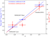 |
Fig. 7. Unabsorbed 0.3–10 keV flux and hydrogen column density versus photon index obtained from MCD+PL model fit. The correlation between F(0.3 − 10) keV and Γ is shown in blue, while correlation between NH and Γ is shown red. The data points were fitted with a linear model and the best-fit model is represented by the dashed lines in the plot. |
Following the studies of Gladstone et al. (2009) on a large sample of ULXs, we also fit the data with a MCD+PL model. As was previously found by Feng & Kaaret (2009) for NGC 5204 X-1 using the same MCD+PL model, we also found a correlation between NH and Γ with a correlation coefficient of 0.93, as shown in Fig. 7 (red points and line). The correlation shows that as Γ increases (simultaneously with the flux), the NH also increases. If this correlation is intrinsic, this might imply that an increase of flux leads to strong outflows from the disk, which, in turn, results in an increase of the hydrogen column density of the disk wind. An additional argument for the possible existence of a wind is that the total hydrogen column density obtained from all our MCD+PL model fits is at least two times higher than the Galactic value for this source (see Sect. 4). This might serve as evidence for the existence of additional intrinsic absorption connected to the source. Nevertheless, a confirmation of the presence of a wind in NGC 5055 X-1 can only come from the analysis of high spectral resolution data from the Grating spectrometers on Chandra and XMM-Newton. We considered available archival data from XMM-Newton reflection gratings (RGS), but the exposure time is too short to obtain any significant detection of emission and absorption lines in NGC 5055 X-1.
In general, the DISKPBB model gives a higher inner disk temperature than the MCD+PL model. The important point to note is that we found T(r) ∝ r−0.5 in all our data sets, which is flatter than expected for a sub-Eddington accretion disk model. Although the source luminosity changes during different epochs of observations, the temperature profile does not respond to such variations (the best-fit values of p are constant). Feng & Kaaret (2007) performed a similar modeling of NGC 1313 X-2 with p as a free parameter, they also obtained high inner disk temperature and p ∼ 0.5. This fact can indicate that the disk in ULX sources may be slim, but a definite answer can only come from a systematic fit of a sample of sources using this model.
The inner temperature, Tin, inferred from MCD+PL and MCD+NTHCOMP models, is relatively low in comparison with the temperature from the DISKPBB model. We plot the luminosity versus Tin for the three models in Figs. 8–10. It is clear that NGC 5055 X-1 follows an inverse relation of luminosity with Tin for all models. The inferred relation is  for the MCD+PL model,
  for the DISKPBB model, and
  for the MCD+NTHCOMP model. This negative correlation is one of the signatures that the emission from the source is geometrically beamed, as has been argued by King (2009). Feng & Kaaret (2007) and Kajava & Poutanen (2009) showed that for power law-type ULXs, the soft-bump follows the relation
  , where n ≈ 3.5. Among our fits, the MCD+PL follows more closely the predicted n ≈ 3.5 trend, although a negative trend is seen in all the other fits. The errors on the inferred relations account for the quite large errors on the temperature. Even considering these errors, the slope of the correlation remains negative, regardless of the model. Of course, the quality of the data and the small number of data points precludes us from obtaining stronger constraints. A longer monitoring period is needed to distinguish among the different models and confirm these conclusions.
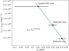 |
Fig. 8. Unabsorbed X-ray luminosity-inner disk temperature relation inferred from the fit of the MCD+PL model. The blue continuous line shows the best fit to the data, which follows the relation |
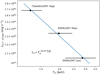 |
Fig. 9. Unabsorbed X-ray luminosity-inner disk temperature relation inferred from the continuum fitting using slim accretion disk DISKPBB model. The blue continuous line shows the best fit to the data, which follows the relation |

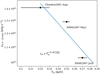 |
Fig. 10. Unabsorbed X-ray luminosity-inner disk temperature relation inferred from the fit of the MCD+NTHCOMP model. The blue continuous line shows the best fit to the data, which follows the relation |

6. Conclusions
In this paper, we analyse the Chandra and XMM-Newton observations of the ULX NGC 5055 X-1. The high luminosity of the source most likely results from the combination of super-Eddington accretion and geometrical beaming. The source does not show much variability across all three observations. Although the quality of the data does not allow us to draw strong conclusions, our spectral fits hint at several interesting results and trends:
(i) NGC 5055 X-1 mostly emits in soft X-rays in the range of 0.3–3 keV, whereas the hard X-ray band flux is only a fraction 0.1–0.3 of the soft X-ray emission, suggesting a dominant thermal component. Therefore, we tested models of emission from an accretion disk around a BH.
(ii) The low inner disk temperature (kTin ∼ 0.25 keV) and the steep power law slope (Γ > 1.5) obtained in some fits may suggest an IMBH. On the other hand, the slim disk model DISKPBB provides a good fit and suggests a temperature emission profile T(r) ∝ r−0.5, which is at odds with that of standard thin disk models (Feng & Kaaret 2007).
(iii) All unabsorbed models confirm that NGC 5055 X-1 is intrinsically extremely luminous, reaching 0.3–10 keV luminosity of 2.32 × 1040 erg s−1. Our analysis slightly favours the scenario that the source is in a soft UL spectral state, but we need better data with longer exposure time to fully confirm this conclusion.
(iv) The flux and NH are positively correlated with the photon index Γ for the MCD+PL model. The source jumps from a steep PL (Γ ≈ 2.4) state to a hard PL state (Γ ≈ 1.8), while NH varies between ∼6 − 16 × 1020 cm−2. This correlation may suggest that the accretion geometry is disk+corona (Cao 2009, and references therein). The increasing absorption column density of hydrogen can be interpreted as an outflow from the disk.
(v) From a physical point of view, the MCD+NTHCOMP model is slightly more favoured since it returns a value of NH consistent with that determined in previous measurements and it allows for a more physical dependency between the two spectral components.
(vi) For all models, we find an inverse relation of X-ray luminosity with inner disk temperature. The errors on the temperature are quite large, but regardless of the fitted model, the slope of this correlation is consistent with being negative within the estimated errors. This result strongly suggests that the source is geometrically beamed. Therefore, we conclude that a plausible explanation for NGC 5055 X-1 is that the source is accreting at a super-Eddington luminosity and that it is beamed by an optically thick wind, as seen in other high luminosity ULXs (King 2009). Further simultaneous broadband observations are needed to constrain the full set of physical parameters for NGC 5055 X-1.
Acknowledgments
We thank the anonymous referee for useful comments that have helped to improve the manuscript. The authors also thank Aneta Siemiginowska for insights into Chandra data reduction process. AR was supported by Polish National Science Center grants No. 2015/17/B/ST9/03422, 2015/18/M/ST9/00541. BDM acknowledges support from the European Union’s Horizon 2020 research and innovation programme under the Marie Skłodowska-Curie grant agreement No. 798726. The work has made use of publicly available data from HEASARC Online Service, Chandra Interactive Analysis of Observations (CIAO) developed by Chandra X-ray Center, Harvard & Smithsonian center for astrophysics (USA), and the XMM-Newton Science Analysis System (SAS) developed by European Space Agency (ESA).
References
- Abramowicz, M. A., Czerny, B., Lasota, J. P., & Szuszkiewicz, E. 1988, ApJ, 332, 646 [NASA ADS] [CrossRef] [Google Scholar]
- Arnaud, K. A. 1996, in XSPEC: The First Ten Years, eds. G. H. Jacoby, & J. Barnes, ASP Conf. Ser., 101, 17 [Google Scholar]
- Bachetti, M., Harrison, F. A., Walton, D. J., et al. 2014, Nature, 514, 202 [NASA ADS] [CrossRef] [Google Scholar]
- Cao, X. 2009, MNRAS, 394, 207 [NASA ADS] [CrossRef] [Google Scholar]
- Carpano, S., Haberl, F., Maitra, C., & Vasilopoulos, G. 2018, MNRAS, 476, L45 [NASA ADS] [CrossRef] [Google Scholar]
- Colbert, E. J. M., & Mushotzky, R. F. 1999, ApJ, 519, 89 [NASA ADS] [CrossRef] [Google Scholar]
- Devi, A. S., Misra, R., Agrawal, V. K., & Singh, K. Y. 2007, ApJ, 664, 458 [CrossRef] [Google Scholar]
- Done, C., & Kubota, A. 2006, MNRAS, 371, 1216 [NASA ADS] [CrossRef] [Google Scholar]
- Fabbiano, G. 1989, ARA&A, 27, 87 [NASA ADS] [CrossRef] [Google Scholar]
- Feng, H., & Kaaret, P. 2006a, ApJ, 653, 536 [NASA ADS] [CrossRef] [Google Scholar]
- Feng, H., & Kaaret, P. 2006b, ApJ, 650, L75 [NASA ADS] [CrossRef] [Google Scholar]
- Feng, H., & Kaaret, P. 2007, ApJ, 660, L113 [CrossRef] [Google Scholar]
- Feng, H., & Kaaret, P. 2009, ApJ, 696, 1712 [CrossRef] [Google Scholar]
- Fürst, F., Walton, D. J., Harrison, F. A., et al. 2016, ApJ, 831, L14 [NASA ADS] [CrossRef] [Google Scholar]
- Fürst, F., Walton, D. J., Stern, D., et al. 2017, ApJ, 834, 77 [NASA ADS] [CrossRef] [Google Scholar]
- Gierliński, M., & Done, C. 2004, MNRAS, 347, 885 [NASA ADS] [CrossRef] [Google Scholar]
- Gladstone, J. C., Roberts, T. P., & Done, C. 2009, MNRAS, 397, 1836 [NASA ADS] [CrossRef] [Google Scholar]
- Gregory, P. C., & Loredo, T. J. 1992, ApJ, 398, 146 [NASA ADS] [CrossRef] [Google Scholar]
- Gronkiewicz, D., & Różańska, A. 2020, A&A, 633, A35 [NASA ADS] [CrossRef] [EDP Sciences] [Google Scholar]
- Heida, M., Torres, M. A. P., Jonker, P. G., et al. 2015, MNRAS, 453, 3510 [NASA ADS] [CrossRef] [Google Scholar]
- Heida, M., Jonker, P. G., Torres, M. A. P., et al. 2016, MNRAS, 459, 771 [NASA ADS] [CrossRef] [Google Scholar]
- HI4PI Collaboration (Ben Bekhti, N., et al.) 2016, A&A, 594, A116 [NASA ADS] [CrossRef] [EDP Sciences] [Google Scholar]
- Hirano, A., Kitamoto, S., Yamada, T. T., Mineshige, S., & Fukue, J. 1995, ApJ, 446, 350 [NASA ADS] [CrossRef] [Google Scholar]
- Huppenkothen, D., Bachetti, M., Stevens, A. L., et al. 2019, ApJ, 881, 39 [CrossRef] [Google Scholar]
- Israel, G. L., Belfiore, A., Stella, L., et al. 2017a, Science, 355, 817 [NASA ADS] [CrossRef] [Google Scholar]
- Israel, G. L., Papitto, A., Esposito, P., et al. 2017b, MNRAS, 466, L48 [NASA ADS] [CrossRef] [Google Scholar]
- Kaaret, P., Corbel, S., Prestwich, A. H., & Zezas, A. 2003, Science, 299, 365 [NASA ADS] [CrossRef] [Google Scholar]
- Kaaret, P., Feng, H., & Roberts, T. P. 2017, ARA&A, 55, 303 [Google Scholar]
- Kajava, J. J. E., & Poutanen, J. 2009, MNRAS, 398, 1450 [NASA ADS] [CrossRef] [Google Scholar]
- Kajava, J. J. E., Poutanen, J., Farrell, S. A., Grisé, F., & Kaaret, P. 2012, MNRAS, 422, 990 [NASA ADS] [CrossRef] [Google Scholar]
- King, A. R. 2009, MNRAS, 393, L41 [NASA ADS] [Google Scholar]
- King, A. R., & Puchnarewicz, E. M. 2002, MNRAS, 336, 445 [CrossRef] [Google Scholar]
- King, A. R., Davies, M. B., Ward, M. J., Fabbiano, G., & Elvis, M. 2001, ApJ, 552, L109 [NASA ADS] [CrossRef] [Google Scholar]
- Kubota, A., & Makishima, K. 2004, ApJ, 601, 428 [NASA ADS] [CrossRef] [Google Scholar]
- Kubota, A., Ebisawa, K., Makishima, K., & Nakazawa, K. 2005, ApJ, 631, 1062 [NASA ADS] [CrossRef] [Google Scholar]
- McQuinn, K. B. W., Skillman, E. D., Dolphin, A. E., Berg, D., & Kennicutt, R. 2017, AJ, 154, 51 [NASA ADS] [CrossRef] [Google Scholar]
- Middleton, M. J., Walton, D. J., Roberts, T. P., & Heil, L. 2014, MNRAS, 438, L51 [NASA ADS] [CrossRef] [Google Scholar]
- Miller, J. M., Fabbiano, G., Miller, M. C., & Fabian, A. C. 2003, ApJ, 585, L37 [NASA ADS] [CrossRef] [Google Scholar]
- Miller, J. M., Fabian, A. C., & Miller, M. C. 2004a, ApJ, 614, L117 [NASA ADS] [CrossRef] [Google Scholar]
- Miller, J. M., Fabian, A. C., & Miller, M. C. 2004b, ApJ, 607, 931 [NASA ADS] [CrossRef] [Google Scholar]
- Mineshige, S., Hirano, A., Kitamoto, S., Yamada, T. T., & Fukue, J. 1994, ApJ, 426, 308 [CrossRef] [Google Scholar]
- Mondal, S., Belczyński, K., Wiktorowicz, G., Lasota, J.-P., & King, A. R. 2020, MNRAS, 491, 2747 [Google Scholar]
- Motch, C., Pakull, M. W., Grisé, F., & Soria, R. 2011, Astron. Nachr., 332, 367 [NASA ADS] [CrossRef] [Google Scholar]
- Motch, C., Pakull, M. W., Soria, R., Grisé, F., & Pietrzyński, G. 2014, Nature, 514, 198 [NASA ADS] [CrossRef] [Google Scholar]
- Petrucci, P. O., Gronkiewicz, D., Rozanska, A., et al. 2020, A&A, 634, A85 [CrossRef] [EDP Sciences] [Google Scholar]
- Pinto, C., Middleton, M. J., & Fabian, A. C. 2016, Nature, 533, 64 [NASA ADS] [CrossRef] [Google Scholar]
- Roberts, T. P., & Warwick, R. S. 2000, MNRAS, 315, 98 [NASA ADS] [CrossRef] [Google Scholar]
- Roberts, T. P., Warwick, R. S., Ward, M. J., & Goad, M. R. 2004, MNRAS, 350, 1536 [NASA ADS] [CrossRef] [Google Scholar]
- Różańska, A., Bresler, K., Bełdycki, B., Madej, J., & Adhikari, T. P. 2018, A&A, 612, L12 [CrossRef] [EDP Sciences] [Google Scholar]
- Shakura, N. I., & Sunyaev, R. A. 1973, A&A, 24, 337 [NASA ADS] [Google Scholar]
- Singha, A. C., & Devi, A. S. 2019, Acta Astron., 69, 339 [Google Scholar]
- Skipper, C. J., & McHardy, I. M. 2016, MNRAS, 458, 1696 [CrossRef] [Google Scholar]
- Stobbart, A. M., Roberts, T. P., & Wilms, J. 2006, MNRAS, 368, 397 [NASA ADS] [CrossRef] [Google Scholar]
- Sutton, A. D., Roberts, T. P., & Middleton, M. J. 2013, MNRAS, 435, 1758 [NASA ADS] [CrossRef] [Google Scholar]
- Swartz, D. A., Soria, R., Tennant, A. F., & Yukita, M. 2011, ApJ, 741, 49 [NASA ADS] [CrossRef] [Google Scholar]
- Tikhonov, N. A., Lebedev, V. S., & Galazutdinova, O. A. 2015, Astron. Lett., 41, 239 [NASA ADS] [CrossRef] [Google Scholar]
- Tully, R. B., Courtois, H. M., Dolphin, A. E., et al. 2013, AJ, 146, 86 [NASA ADS] [CrossRef] [Google Scholar]
- Watarai, K.-Y., Fukue, J., Takeuchi, M., & Mineshige, S. 2000, PASJ, 52, 133 [NASA ADS] [CrossRef] [Google Scholar]
- Zdziarski, A. A., Johnson, W. N., & Magdziarz, P. 1996, MNRAS, 283, 193 [NASA ADS] [CrossRef] [Google Scholar]
- Życki, P. T., Done, C., & Smith, D. A. 1999, MNRAS, 309, 561 [NASA ADS] [CrossRef] [Google Scholar]
All Tables
All Figures
|
Fig. 1. X-ray image in counts per pixel displays the field of view of Chandra ACIS-S (left panel) and XMM-Newton EPIC-MOS1 (2007-05-28; right panel) detectors. The green circles containing bright pixels show NGC 5055 X-1, while the empty green circles represent the region from where the background was extracted. Chandra spatial resolution allowed us to extract source photons from a circular region of 6″ radius, while for XMM-Newton we used circular regions of 40″. |
| In the text | |
|
Fig. 2. Chandra ACIS-S and XMM-Newton EPIC-PN light curves of NGC 5055 X-1 for the three observations at different epochs (observation IDs are indicated in each panel). Soft 0.3–3 keV and hard 3–10 keV energy band light curves are shown in the upper and middle panels, respectively, while the bottom panels show the hardness ratios for each set of data. All the light curves are re-binned with bin size 500 s to have higher S/N. The zero times in the plots correspond to 2001-08-27 02:13:48, 2007-05-28 07:59:14, and 2007-06-19 10:56:29 for panels from left to right, respectively. |
| In the text | |
|
Fig. 3. Chandra observation probability-weighted light curves, as obtained from the CIAO glvary tool, i.e. after taking account all instrumental effects. The zero time corresponds to 2001-08-27 02:13:48. The total probability of variability for the 0.3–3 keV and 3–10 keV light curves is 0.02 and 0.07, respectively (see Sect. 3). |
| In the text | |
|
Fig. 4. Ratio of data to the folded model obtained from the fit of a MCD model, using DISKBB in XSPEC. The MCD model clearly leaves an excess at high energies. In XMM-Newton panels, the black, red, and green data points are, respectively, the spectra from EPIC-PN, EPIC-MOS1, and EPIC-MOS2. |
| In the text | |
|
Fig. 5. Each subplot shows the data with the folded model in the upper panel and the data-to-model ratio in the lower panel. In the first row, results from the fit of the MCD+PL model are presented, in the second row the DISKPBB model, and, finally, in the third row we have MCD+NTHCOMP. The different columns correspond to Chandra data in the left column, XMM-Newton 2007-05-28 data in the middle column, and 2007-06-19 data in the right column. |
| In the text | |
|
Fig. 6. Unfolded absorbed models (solid lines) and model components (dot-dashed line for MCD and dashed line for NTHCOMP and PL) fitted to the XMM-Newton 2007-06-19 data. Red lines represent the MCD+PL model, the blue line is the DISKPBB model, and green lines show the MCD+NTHCOMP model in which the MCD component is the most prominent. |
| In the text | |
|
Fig. 7. Unabsorbed 0.3–10 keV flux and hydrogen column density versus photon index obtained from MCD+PL model fit. The correlation between F(0.3 − 10) keV and Γ is shown in blue, while correlation between NH and Γ is shown red. The data points were fitted with a linear model and the best-fit model is represented by the dashed lines in the plot. |
| In the text | |
|
Fig. 8. Unabsorbed X-ray luminosity-inner disk temperature relation inferred from the fit of the MCD+PL model. The blue continuous line shows the best fit to the data, which follows the relation |
| In the text | |
|
Fig. 9. Unabsorbed X-ray luminosity-inner disk temperature relation inferred from the continuum fitting using slim accretion disk DISKPBB model. The blue continuous line shows the best fit to the data, which follows the relation |
| In the text | |
|
Fig. 10. Unabsorbed X-ray luminosity-inner disk temperature relation inferred from the fit of the MCD+NTHCOMP model. The blue continuous line shows the best fit to the data, which follows the relation |
| In the text | |
Current usage metrics show cumulative count of Article Views (full-text article views including HTML views, PDF and ePub downloads, according to the available data) and Abstracts Views on Vision4Press platform.
Data correspond to usage on the plateform after 2015. The current usage metrics is available 48-96 hours after online publication and is updated daily on week days.
Initial download of the metrics may take a while.