| Issue |
A&A
Volume 690, October 2024
|
|
|---|---|---|
| Article Number | A335 | |
| Number of page(s) | 11 | |
| Section | Extragalactic astronomy | |
| DOI | https://doi.org/10.1051/0004-6361/202449509 | |
| Published online | 22 October 2024 | |
Exploring the nature of an ultraluminous X-ray source in NGC 628
Adiyaman University, Department of Physics, 02040 Adiyaman, Türkiye
Received:
6
February
2024
Accepted:
6
August
2024
Abstract
Aims. In this work, we study the X-ray spectral and temporal properties of an ultraluminous X-ray source (ULX) in NGC 628 by using multi-epoch archival X-ray data. The physical parameters were estimated in each epoch in order to constrain the nature of the compact object in the system. Also, the optical counterpart candidates of the ULX were examined using the archival Hubble Space Telescope (HST)/Wide Field Camera 3 (WFC3) data.
Methods.XMM-Newton, Chandra, and Swift data were used to create the long-term light curve (which covers a period of 22 years) and perform the spectral analysis. Lomb-Scargle periodograms of the source were constructed to examine the short-term variability in each epoch. In order to search for an optical counterpart in the HST/WFC3 images, a relative astrometric correction was initially applied to the Chandra and HST/WFC3 images.
Results. The X-ray flux of the source changes by a factor of ∼200 throughout the observations. The previously detected quasi-periodic signal (in the range of 0.1−0.4 mHz) was confirmed by using the Lomb-Scargle method. After astrometric correction, two optical counterpart candidates were detected for the source. The obtained spectral energy distributions in the optical band for both candidates indicate that the optical emission is dominated by the irradiation of the accretion disc. Considering the best-fit model parameters of the multi-colour disc black-body model, we derived the mass of the black hole in the system as being in the range of (5−28) M⊙. Nonetheless, the long-term variability and the spectral transitions in the hardness–luminosity diagram make it difficult to rule out the neutron star scenario.
Key words: galaxies: individual: NGC 628
Corresponding author; This email address is being protected from spambots. You need JavaScript enabled to view it.
© The Authors 2024
 Open Access article, published by EDP Sciences, under the terms of the Creative Commons Attribution License (https://creativecommons.org/licenses/by/4.0), which permits unrestricted use, distribution, and reproduction in any medium, provided the original work is properly cited.
This article is published in open access under the Subscribe to Open model. This email address is being protected from spambots. You need JavaScript enabled to view it. to support open access publication.
1. Introduction
Ultraluminous X-ray Sources (ULXs) are generally defined as extra-Galactic, point-like X-ray sources with X-ray luminosities exceeding the Eddington limit for a typical stellar mass black hole (BH) of 10 M⊙ (∼2 × 1039 erg s−1), and they are located outside their host galaxy nucleus. Even though the true nature of ULXs is still being debated, there are several basic models in the literature that explain the high luminosities of these sources. To explain their high luminosity, ULXs were initially thought to be systems that contain an intermediate-mass black hole (IMBH; 102 − 105 M⊙) accreting at sub-Eddington rates (Colbert & Mushotzky 1999; Miller et al. 2004; Farrell et al. 2009). In contrast, some studies have suggested that these systems contain stellar-mass black holes (SMBHs) and are powered by super-Eddington accretion and/or strong beamed emission (e.g. King et al. 2001; Feng & Soria 2011; Walton et al. 2013; Middleton et al. 2015). Recently, the detection of pulsation in the M82 X-2 revealed that ULXs may contain neutron stars (Bachetti et al. 2014). With the increasing number of pulsating ULXs (PULXs) that have been detected (Fürst et al. 2016; Israel et al. 2017a,b; Pintore et al. 2017; Koliopanos et al. 2017; Walton et al. 2018; Sathyaprakash et al. 2019; Rodríguez Castillo et al. 2020; Gúrpide et al. 2021), it is thought that most of the ULXs could be super-Eddington accretion systems containing SMBHs or neutron stars rather than IMBHs.
Investigating the X-ray spectral and timing properties of ULXs provides important information for constraining the mass of the compact object (accretor) and understanding the accretion regime. The spectrum of the vast majority of ULXs differs from Galactic black hole binaries (GBHBs), where the accretion usually occurs at a sub-Eddington rate. Typically, ULXs have a soft excess coupled with a spectral curvature below 10 keV. In contrast to ULXs, this curvature is generally seen at higher energies (> 10 keV) in GBHBs. Besides, the super-Eddington models predict strong outflows (e.g. Poutanen et al. 2007), and the recent detections of blueshifted lines in the spectra of many ULXs when using the data taken with the Reflection Grating Spectrometers (RGS) instrument aboard XMM-Newton have revealed the existence of outflows (e.g. Pinto et al. 2016). Thus, the spectra of ULXs support the super-Eddington accretion scenario rather than sub-Eddington accretion (Pinto & Walton 2023; Pinto & Kosec 2023 and references therein). In addition, ULXs exhibit different spectral states that are generally defined in three categories: soft ultraluminous, hard ultraluminous, and broadened disc (Sutton et al. 2013). When the spectrum of the source is modelled with a thermal plus a power-law component, the spectral state is classified as soft ultraluminous (Γ > 2) or hard ultraluminous (Γ < 2), depending on the spectral index. If the spectrum is dominated by the disc component, its spectral state is defined as a broadened disc (Sutton et al. 2013). Moreover, Sutton et al. (2013) found that the ULXs in the hard and soft ultraluminous spectral state are generally brighter.
The optical counterparts of ULXs also play an important role in estimating the spectral class and mass of the companion star and origin of the optical emission itself. Studies using the Hubble Space Telescope (HST) data show that the optical counterparts of most ULXs are faint, and usually their apparent magnitudes are in the range of 21 ≤ mV ≤ 26 (Fabrika et al. 2021). Since their visual magnitudes are very dim and they are usually located in crowded regions (such as star-forming regions), the number of ULXs that were associated with an optical counterpart is only around 30 (Kaaret et al. 2017; Fabrika et al. 2021). Considering the luminosity and colour values of their optical counterparts, the companion stars of many ULXs are massive stars with an O or B spectral type; thus, they can be classified as high-mass X-ray binaries (Liu et al. 2002, 2004; Terashima et al. 2006; Gladstone et al. 2013). On the other hand, some ULXs have companion stars with an A or late type, and they can be classified as low-mass X-ray binaries (Tao et al. 2011; Avdan et al. 2016b, 2019).
The aim of this paper is to study the X-ray properties of the ULX (hereafter X-1) in NGC 628 (M 74) in detail. We re-analysed the XMM-Newton and Chandra observations that were previously used in the literature to study X-1 as well as the newer XMM-Newton, Chandra, and Swift archival data, which had not been used for this purpose before. Additionally, the optical counterpart of X-1 was searched for using the HST/Wide Field Camera 3 (WFC3) archival data. NGC 628 is a star-forming, face-on spiral galaxy with an inclination angle of ∼(5−7)° (Shostak & van der Kruit 1984) at a distance of 9.7 Mpc (Tully 1988). X-1 is located in a spiral arm and is to the south-east of the nucleus. X-1 was uncatalogued in the ROSAT and Einstein catalogues, and it was classified for the first time as a bright transient X-ray source with a luminosity of 5 × 1039 erg s−1 in the XMM-Newton observation by Soria & Kong (2002). Later, Krauss et al. (2005) investigated the temporal and spectral variation of X-1 using two Chandra observations and one from XMM-Newton. In these observations, the luminosity of X-1 varied from 5 × 1038 to 1.2 × 1040 erg s−1 across about eight months. This extreme variability and spectral state transition of the source are similar to Galactic microquasars, which supports the idea that the origin of the high luminosity of X-1 could be relativistically beamed jets. Also, the authors speculated that the source may contain an IMBH based on the calculated low disc temperature values. Liu et al. (2005) determined a two-hour quasi period in X-1 by using two Chandra and two XMM-Newton observations. Then they calculated the mass of the BH in the system as ∼104 M⊙ using the fb − M⚫ scaling relation, where fb is the break frequency.
This paper is organised as follows. The observations and data reduction steps are described in Sect. 2; the result of the X-ray and optical analyses and the discussions are given in Sect. 3; and the summary is given in Sect. 4.
2. Observations and data reductions
NGC 628 was observed multiple times with XMM-Newton, Chandra, and Swift over 22 years. It has also been observed with different HST cameras. We used the F275W, F336W, F555W, and F814W data taken with the WFC3 to investigate the optical counterpart of the ULX X-1. The details of the observations used in this study are summarised in Table 1. The Sloan Digital Sky Survey (SDSS) image of NGC 628 and the HST image around X-1 are given in Fig. 1.
Archival observations used in this work.
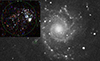 |
Fig. 1. Sloan Digital Sky Survey and HST true colour (zoomed) images of NGC 628 (red: F555W; green: F336W; blue: F275W). The green circle represents a 7″ area around X-1, and the corrected position of X-1 is shown with green bars in the zoomed-in HST image. |
2.1. X-ray observations
We analysed the XMM-Newton data using the standard software tools of SAS1 (XMM-Newton Science Analysis System) v21.0 (Gabriel et al. 2004) and the latest Current Calibration Files (CCF) files were used for re-calibration. To create the calibrated event files, the EPCHAIN and EMCHAIN tasks were used for the EPIC PN and MOS cameras, respectively. After all the event files were obtained in the 0.3−10 keV energy range, the source and background counts were extracted from circular regions of 30″ and 60″ in radius using the EVSELECT task, respectively. The background regions were selected on source-free regions. The light curves of the source were also constructed using the ETIMEGET procedure in SAS. In XM1 and XM2 observations (see Table 1), almost half of the X-1 counts fall on the chip gap in the EPIC PN frames. Therefore, we used only MOS data when analysing these two observations. For XM3, we used both PN and MOS data.
The data reduction of the Chandra observations was performed using the Chandra Interactive Analysis of Observations (CIAO) v4.12 software package2 and the Chandra Calibration Database (CALDB) v4.9.3 calibration files (Fruscione et al. 2006). X-1 was located on the ACIS S3 (back-illuminated) chip. Using the CHANDRA_REPRO script, the event files were created in the soft, hard, and total energy bands: 0.3−1.5 keV – soft (S), 1.5−10 keV – hard (H), 0.3−10 keV – total (T). At all energy ranges, the source and background counts were obtained using the SPECEXTRACT task from circular regions of 5″ and 10″ in radius, respectively. The background photons were extracted from a location with no source contamination. The light curves were constructed using the DMEXTRACT task in CIAO in the total energy range.
The source was observed by the Swift/X-ray Telescope (XRT) 54 times between 2001 and 2023. The energy spectra of the source were extracted with the XSELECT tool (v2.4) in the HEASOFT package (Blackburn 1995). While extracting the spectra, 35″ circular regions were selected both for the source and background. The spectral files were obtained in the 0.3−10 keV energy range. Due to insufficient statistics, only the net count rate of X-1 was calculated in the Swift data while examining the long-term variability of the source.
2.2. HST observations and astrometry
We used the HST/WFC3/UVIS observations to investigate the optical properties of the possible optical counterpart(s) of X-1. To search for optical counterpart candidates of the ULX in HST images, the relative astrometry between the Chandra and HST images was improved. The HST/WFC3 F336W (H2) drizzled image and C11 data were used to calculate the coordinate difference. Two reference sources that were detected by both telescopes were chosen while determining the relative shifts between two images. Then the shifts in R.A. and Dec values were applied in order to calculate the corrected position of the ULX on the HST image. The corrected position of the source was estimated as RA = 01:36:51.0766, Dec = +15:45:46.968 in the HST/WFC3 F336W drizzled image with an uncertainty of 0.3″.
We performed point spread function (PSF) photometry using the DOLPHOT v2.0 software. The data files used in this study were taken from the HST data archive3. Stellar photometry was done by following the steps in the DOLPHOT manual (Dolphin 2000, 2016) using the HST/WFC3 images. We used the WFC3MASK and CALCSKY tasks so that bad pixels were masked in the images and a sky image was created. Then the DOLPHOT task was run to detect the possible optical sources and to perform photometry. The default DOLPHOT zero points and aperture corrections were adopted during the calculations.
Determining the optical counterparts of ULXs allowed us to constrain the age and mass of the donor star. If it is assumed that the optical emission is dominated by the donor star, it is possible to determine the age of the donor star using theoretical isochrones. To estimate the mass of the donor stars, we obtained the colour–magnitude diagrams (CMDs) of the possible optical candidates of X-1. Using the Padova and Trieste Stellar Evolution Code (PARSEC)4 isochrones for the HST/WFC3 wide filters, the CMD (F555W-F814W versus F555W) was created for the possible optical counterpart(s) and field stars located within 7″ around of X-1 (Fig. 8). While obtaining the CMD, we adopted the metallicity at solar value and the distance modulus as 29.9 mag. The PADOVA isochrones were corrected for the reddening of E(B − V) = 0.15 mag.
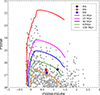 |
Fig. 8. Colour–magnitude diagram of X-1 from HST/WFC3. The optical counterpart candidate (c1) is shown as colourful stars in different observations, and field stars within 7″ around X-1 are shown as grey circles. The black, red, and blue colours represent magnitudes of c1 calculated using H4, H6, and H8 data, respectively. The PADOVA isochrones with different ages have been corrected for extinction of AV = 0.46 mag. |
3. Results and discussion
For this study, we investigated the X-ray spectral and temporal properties of X-1 in NGC 628 in detail using archival X-ray observations. NGC 628 has archival observations by XMM-Newton, Chandra, and Swift spanning 22 years. While many of these observations were used for the first time to study X-1, some of the data (XM1, XM2, C1, and C2 in Table 1) were re-analysed. Additionally, we searched the optical counterpart for X-1 using the archival HST/ WFC3 data and determined two optical counterpart candidates within the estimated error radius.
3.1. X-ray spectral analysis
The spectral analyses of XMM-Newton and Chandra data were carried out in the 0.3−10 keV energy band using XSPEC v12.13.1 (Arnaud 1996). Prior to fitting, all spectra of X-1 were grouped to have a minimum of 20 counts per energy bin using the GRPPHA task. The spectra were then fitted with the power law (PO) and multi-colour disc black-body (DISKBB) models by multiplying with the absorption model (TBABS) twice. While one of the absorption components was fixed to the Galactic value (0.05 × 1022 cm−2, Dickey & Lockman 1990), the other was left free to derive the intrinsic absorptions. The flux values were calculated using the CFLUX convolution model in the 0.3−10 keV energy range. The best-fit model parameters are given in Table 2.
Best-fit X-ray spectral parameters of X-1 in all epochs calculated with TBABS*TBABS*PO and TBABS*TBABS*DISKBB models.
The spectra of the source are generally well modelled with the PO model. The best-fit photon index (Γ) values slightly changed over the years, ranging from 1.52 to 2.14. Nonetheless, the luminosity of the source significantly changed by a factor of approximately ten. This trend can also be seen from the obtained Γ − LX plot (Fig. 2), where Γ values are the spectral index derived from the PO model and LX values are the unabsorbed luminosities in the 0.3−10 keV energy range. We performed a Pearson regression test to check whether any correlation is present between the two quantities (see Fig. 2) using the SCIPY package (Virtanen et al. 2020). The test did not yield any significant correlation (with a p value ∼0.3).
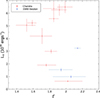 |
Fig. 2. Best-fit Γ versus luminosity diagram of X-1. The Γ values are derived from the PO model, and the luminosities were calculated in the 0.3−10 keV energy band. |
We also fitted the spectra of X-1 with the PO+DISKBB model to determine the spectral regime, whether soft ultraluminous, hard ultraluminous, or broadened disc (three empirical classification for ULXs by Sutton et al. 2013), in each epoch. Due to the low statistical quality, the parameters were poorly constrained except for the high-quality XM3 data. The best-fit model parameters derived the using XM3 data are given in Table 3. Considering the best-fit parameters in Table 3 and by following the criteria given by Sutton et al. (2013), the spectral state of NGC 628 X-1 in XM3 data can be classified as hard ultraluminous.
Best-fit parameters obtained from the TBABS*TBABS*(PO+DISKBB) model for the spectrum of X-1 in XM3 data.
Usually, the spectra of ULXs are fitted with an extended disc black-body model (DISKPBB in XSPEC) (Kubota et al. 2005) in order to determine if the accretion disc is a standard disc (Shakura & Sunyaev 1973) or a slim disc (Abramowicz et al. 1988; Watarai et al. 2001). In the DISKPBB model (also known as the p-free model), the relation between disc temperature and radius is given by T(R)∝Rp, where for a standard disc with sub-Eddington accretion, p ∼ 0.75. On the other hand, when the accretion rate increases near or above the super-Eddington regime, the disc becomes an advection-dominated slim disc, and the p value reaches ∼0.5 (Watarai et al. 2000; Poutanen et al. 2007). We fitted the XM3 data that has the highest statistical quality with the DISKPBB model. The best-fit model parameters are given in Table 4, and the obtained energy spectrum of X-1 with the best-fit model is shown in Fig. 3. The yielded p value (0.5) indicates that the accretion disc in X-1 exhibits slim disc properties. Also, the inner disc temperature value calculated from the model (kTin ∼ 2.4 keV) is very high, as seen in some ULXs (Vierdayanti et al. 2006; Gladstone et al. 2009; Isobe et al. 2012; Pintore et al. 2016, 2020). The high temperature values are consistent with the slim disc model since the spectral hardening factor, κ, is considered to be higher in the case of a slim disc compared to a standard disc (Watarai & Mineshige 2003).
Best-fit parameters obtained from the TBABS*TBABS*DISKPBB model for the spectrum of X-1 in XM3 data.
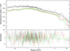 |
Fig. 3. XMM-Newton PN (black), MOS1(red), and MOS2 (green) energy spectrum of X-1 obtained using XM3 data. The spectrum was fitted with the TBABS*TBABS*DISKPBB model. |
The mass of the compact object in X-1 can be estimated using the normalisation parameter calculated from the DISKPBB model. The apparent inner disc radius (rin) can be obtained by considering the normalisation parameter (N) with the following equation:
 (1)
(1)
where i is the inclination and D is the distance in units of 10 kpc (Makishima et al. 2000). The relation between the true (Rin) and apparent inner disc radius (rin) is given by
 (2)
(2)
where the correction factor is ξ = 0.353 (Vierdayanti et al. 2008) and the spectral hardening factor is κ = 3 (Watarai & Mineshige 2003) for a slim disc.
For the spectrum of X-1 in XM3 data, the best-fit DISKPBB normalisation parameter was calculated as N = (5.93 ± 0.05)×10−5. Assuming a moderate inclination of i = 60°, the true inner disc radius for X-1 is estimated as ∼35 km via Eqs. (1) and (2). We then used the relation between the mass and inner disc radius (Makishima et al. 2000) by multiplying it with the minimum mass correction factor (1.2) for a slim disc (Vierdayanti et al. 2008):
 (3)
(3)
where α = 1 for a non-rotating Schwarzschild BH and α = 1/6 for an extremely rotating Kerr BH. Therefore, we derived the mass of the compact object in X-1 as (5 − 28) M⊙ for both cases.
3.2. X-ray temporal analysis
The source exhibits quasi-periodic oscillation (QPO), which was detected previously in XM1, C1, and C2 data (0.1−0.4 mHz, Liu et al. 2005). We used the Lomb-Scargle method (Lomb 1976; Scargle 1982) in order to search for this QPO feature in other observations and to examine the short-term variability in the XMM-Newton and Chandra observations. The PN, MOS1, and MOS2 light curves of the source were combined with the LCMATH tool in the HEASOFT package, and the combined light curves were used throughout the timing analyses of all the XMM-Newton observations. The Lomb-Scargle periodograms of the source were computed over the whole frequency range for each background-subtracted data by using the LOMBSCARGLE tool (VanderPlas et al. 2012; VanderPlas & Ivezić 2015) within the ASTROPY package (Astropy Collaboration 2022). The 3σ false alarm probability levels were estimated by following the method of Baluev (2008) and the bootstrap approach. The number of samples was set to 1000 when using the bootstrap method.
The Lomb-Scargle periodograms of the source show significant QPO features (> 3σ) in XM1, C1, C2, C9, and C10 data within the frequency range of f = (1 − 3)×10−4 Hz. The obtained periodograms are shown in Fig. 4. The solid and dashed lines in each panel represent the estimated 3σ false alarm probability levels computed with both methods. The centroid frequencies of the features are in good agreement with the previous results of Liu et al. (2005).
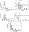 |
Fig. 4. Lomb-Scargle periodograms of X-1 obtained using XM1, C1, C2, C9, and C10 data. The black dashed and solid lines represent the 3σ false alarm levels estimated with the method of Baluev (2008) and the bootstrap approach, respectively. The centroid frequency values of the significant peaks are given in each panel. |
Some ULXs are known to contain neutron stars via detection of pulsations (PULXs; Bachetti et al. 2014; Fürst et al. 2016; Israel et al. 2017b; Carpano et al. 2018; Sathyaprakash et al. 2019; Rodríguez Castillo et al. 2020; Quintin et al. 2021). The known PULXs generally exhibit a harder spectrum and significant long-term variability (Pintore et al. 2017; Gúrpide et al. 2021). This long-term variability is sometimes in a structure of bimodal flux distribution, which may be explained by the onset of the propeller regime (e.g. Tsygankov et al. 2016). Although we were not able to detect any similar pulsations, we compared the properties of the source with the properties of the well-known PULXs. The long-term light curve of X-1 and the histogram of the luminosities are given in Fig. 5. Since the source has insufficient statistics to perform a spectral fitting in Swift and two Chandra (C3 and C4) observations, the count rates of the source in these observations were converted to unabsorbed flux values using the Portable, Interactive Multi-Mission Simulator (PIMMS)5. While performing the conversion, a power-law model was used by adopting the average Γ value (∼1.9) from Table 2, and the Galactic absorption was taken as 0.05 × 10⁻²² cm−2(Dickey & Lockman 1990). The light curve indicates that the source is variable, and the luminosity value of X-1 changed by a factor of ∼200 between the years 2001 and 2023.
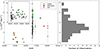 |
Fig. 5. Long-term light curve (left) and the histogram of the derived luminosities (right) of X-1 using the Chandra, XMM-Newton, and Swift data. The luminosity values were calculated in the 0.3−10.0 keV energy band. The inner panel in the light curve was given to separate the Chandra and Swift data for clarity. |
In addition, we obtained a hardness-luminosity diagram (HLD) for X-1 (Fig. 6), using all the available XMM-Newton and Chandra observations. While deriving the hardness ratio, the unabsorbed fluxes were calculated within the range of 0.3−1.5 keV and 1.5−10 keV for the soft and hard bands, respectively. The arrows in Fig. 6 indicate the transitions between the observations. In a recent study, HLDs of 17 ULXs were obtained and compared in order to constraint the nature of the compact source (Gúrpide et al. 2021). They suggested that harder sources could harbour a strongly magnetised neutron star, whereas the softer ones could contain weakly magnetised neutron stars or BHs. Regarding the comparison of the X-1 HLD with that of the HLDs of ULXs in Gúrpide et al. (2021), we found that X-1 shows similarities with NGC 1313 X-2 (which exhibits softer spectra similar to NGC 628 X-1). Considering the variability and the similarity between the HLDs, the neutron star scenario for X-1 cannot be ruled out.
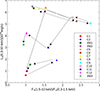 |
Fig. 6. Hardness-luminosity diagram of X-1. Temporal tracks are indicated by arrows. Each epoch is shown with different colours and symbols. |
3.3. Optical counterparts
After the astrometric correction, two optical counterpart candidates (c1 and c2) were found within the error radius of 0 3. The corrected position of X-1 and the counterpart candidates are shown in Fig. 7. Although c1 was detected in all observations, c2 was not detected in the F814W filter images. The de-reddened HST/WFC3 magnitudes of c1 and c2 are given in Table 5. In a previous study, the unique optical counterpart of X-1 was identified within the error radius after astrometric correction using the HST/ACS data (Avdan et al. 2023b). This counterpart coincides with source c1. Although the HST/WFC3 data are statistically better than previous observations, c1 and c2 sources were not detected in the WFC3/F438W filter (H3 observation in Table 1). Therefore, we adopted the previous ACS/F435W (B) magnitude of c1, which was calculated by Avdan et al. (2023b), in the following calculations for c1.
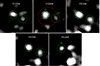 |
Fig. 7. Images from HST/WFC3 of the corrected positions of X-1 in three simultaneous filters (H1, H2 and H3, upper panel) and two simultaneous filters (H4 and H5, lower panel). The images have a size of 1″ × 1″. The red dashed circle shows the astrometric error radii (0 |

De-reddened magnitude values of the optical counterpart candidates of X-1 obtained with HST/WFC3 data.
The absolute magnitudes of c1 and c2 were calculated as being in the range MV = ( − 4.1)−(−3.6) and ( − 3.7)−(−3.1), respectively. Although the absolute magnitudes of both optical candidates are slightly dim, they are compatible with the values of previously studied ULXs (−8 < MV < −3, Kaaret et al. 2017; Fabrika 2017). Assuming that the donor star dominates the optical emission and using the absolute magnitudes and colour values, (V − I)0, the spectral types of c1 were determined as being F−G type giant/supergiant (Straizys & Kuriliene 1981; Ducati et al. 2001), and this is consistent with the previous study (Avdan et al. 2023b). The spectral type for c2 could not be calculated due to a lack of F438W (B) and F814W (I) magnitudes (which was also not detected in previous observations).
X-1 is located in a crowded region, but no star clusters associated with the source have been identified (Avdan et al. 2023b). Considering the CMD given in Fig. 8, if the optical emission comes from the donor star, the age of the star in this system is determined as ≥60 Myr. It can be seen that the field stars are divided into bright-young stars and older-fainter stars. The ages of the young and bright stars are 10−25 Myr, and their (V − I) colour values are between −0.2 and 0.5. The colour values of the older ones are between 0.1 and 2.0, and the colours of c1 are within this range as well.
It is known that the optical emission from ULXs can be dominated by a companion star and/or the accretion disc. There are a few helpful derivations that have been used to constrain the nature of the optical emission. The X-ray–to–optical flux ratio (ξ) can be used as a distinguishing parameter between low-mass X-ray binaries (LMXBs) and high-mass X-ray binaries (HMXBs). It is defined by van Paradijs & McClintock (1995) as ξ = B0 + 2.5 × log FX, where B0 is the de-reddened B magnitude and FX is the X-ray flux in the 2−10 keV energy range in units of microjansky. Most ULXs have very high ξ values (ξ ≥ 20), indicating that the origin of optical emission from ULXs is similar to LMXBs rather than HMXBs (Tao et al. 2011; Avdan et al. 2019). This high value shows that the optical emission comes from the irradiated accretion disc. Since c1 does not have a WFC3/F438W magnitude, we calculated the ξ value as ∼21 by adopting the ACS/F435W magnitude (mF435W = 25.6, Avdan et al. 2023b). Due to a lack of simultaneous optical and X-ray observations, the flux value obtained from the XM2 observation (closest to the ACS/F435W observation) was used. In addition, by considering the high X-ray flux variability of X-1, the ξ was calculated as 20.4 and 21.9 using the lowest derived flux (XM1) and the highest derived flux (C8) in the 2−10 keV energy band, respectively. In any case, the origin the optical emission of c1 is similar to LMXBs rather than HMXBs.
Another X-ray–to–optical flux ratio is defined as log(FX/Fopt) = log FX + mV/2.5 + 5.37 (Maccacaro et al. 1982), where FX is the unabsorbed X-ray flux value in the 0.3−3.5 energy band, mV is the extinction-corrected visual magnitude. This ratio allows one to distinguish the active galactic nuclei (AGNs), BL Lac object, and cluster of galaxies. For these objects, this ratio is determined as being between −1 and 1.7 (Maccacaro et al. 1982; Stocke et al. 1991). Using C9 and H3 observations, the log(FX/Fopt) values of c1 and c2 were calculated as 3.2 and 3.4, respectively. These ratios are greater than the ratios of AGNs, BL Lac objects, and cluster of galaxies, and they are similar to the optical counterparts of known ULXs (Yang et al. 2011; Avdan et al. 2016a, 2023a).
We also calculated the optical spectral index αox for the optical counterpart candidates as described by Sonbas et al. (2019) (and references therein). This parameter gives the correlation between the UV flux density at 2500 Å and the X-ray flux density at the 2 keV energy band. In each data, the X-ray flux density values of the ULX were obtained with a power-law model. By coupling each X-ray data with the only available HST/F275W observation (H1 in Table 1), the αox values for c1 and c2 were calculated. The obtained αox values for c1 and c2 using each X-ray data are given in Cols. 7−8 in Table 2. The αox for c1 and c2 were determined as being in the range of [−0.60, −0.21] and [−0.55, −0.16], respectively. These values are compatible with those found for the ULXs examined by Sonbas et al. (2019) (see Table 1 and Fig. 1 in their paper).
The spectral energy distributions (SEDs) were constructed using the HST observations with the F275W, F336W, F555W, and F814W filters for c1 and the F275W, F336W, and F555W filters for c2. The obtained SEDs are shown in Fig. 9. The distributions of both counterpart candidates are consistent with a single power law (Fν ∝ να), similar to many ULXs (Tao et al. 2011; Vinokurov et al. 2013, 2018; Aksaker et al. 2019). The index value of the power-law models for the SEDs of c1 and c2 are α = −0.67 ± 0.26 and α = −0.14 ± 0.05, respectively. The SEDs with power-law index values between about −1 and 2 indicate that the optical emission is dominated by irradiation in the outer disc rather than the donor star.
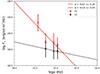 |
Fig. 9. Spectral energy distributions of the optical counterpart candidates for X-1. The c1 and c2 data are given as red squares and black circles, respectively. The SED models for c1 and c2 are shown as red solid and black dashed lines, respectively. The power-law indexes are α = −0.67 ± 0.26 for c1 and α = −0.14 ± 0.05 for c2. |
X-1 has four F555W observations between 2013 and 2021 (H3, H4, H6, and H8 data in Table 5), and these allowed us to investigate the long-term magnitude variation of the counterpart candidates. The magnitude difference in the F555W (V) bands, Vmin − Vmax, for both candidates was calculated as 0.57 ± 0.19 for c1 and 0.61 ± 0.55 for c2. Similar high magnitude variations in the optical band that were seen in some ULXs were found to be correlated with the X-ray flux (Soria et al. 2012; Vinokurov et al. 2020). Unfortunately, we could not compare the optical variability of X-1 with its X-ray flux due to the lack of simultaneous (or quasi simultaneous) X-ray and optical data. The high variability in colour and absolute magnitude, ξ value, and the high Vmin − Vmax value of c1 indicate that the optical emission from this source is dominated by an irradiated accretion disc (Tao et al. 2011; see Tables 5 and 6 in their paper). Although c2 has a higher Vmin − Vmax, it is unreliable due to a high error value. Also, the fact that the source c2 is not detected in the F435W (B) and F814W (I) filters limits our knowledge about this source. However, it is difficult to ignore this source as an optical counterpart of X-1. Additional HST observations with different filters are required to investigate its optical properties in more detail.
4. Summary
We have examined the X-ray properties of ULX X-1 in detail by using the available X-ray data of NGC 628. The previously reported XMM-Newton and Chandra observations were also re-analysed. To study the optical emission of X-1, we used the archival HST/WFC3 data. Below, we present a list that summarises the results.
-
The X-ray spectra of X-1 are generally well fit with PO, with the spectral indexes in the range of Γ = 1.5 − 2.1. In XM3 data, which provides the highest statistics, the spectra are also well fit with the PO+DISKBB and DISKPBB models. For the former, the disc temperature is compatible with kTin ≈ 0.4 keV, while for the latter it is kTin ≈ 2.4 keV.
-
The previously detected QPO signal in X-1 was confirmed and detected in some of the newer datasets by using the Lomb-Scargle method. The frequency of the QPO signal is in the range of f = (1 − 4)×10−4 Hz.
-
The spectrum of X-1 yielded a good fit with the DISKPBB model, and the best-fit p value (0.5) shows that the accretion disc exhibits slim disc properties. The mass of the BH in X-1 was derived as (5−28) M⊙ by considering the DISKPBB model.
-
The source exhibits a long-term variability by a factor of ∼200 throughout the observations. The HLD of the source looks similar to the HLD of the previously studied PULX NGC 1313 X-2. This similarity makes it difficult to rule out the neutron star scenario for the nature of the compact object in X-1. The fact that the spectrum of the source is rather softer relative to other PULXs indicates that it may contain a weakly magnetised neutron star.
-
After astrometric correction, two optical counterpart candidates (c1 and c2) were identified for X-1. While c1 was detected in all observations but H10; c2 was not detected in the F814W and H10 observations.
-
The c1 and c2 candidates are both brighter in the UV. The absolute magnitudes are MV ∼ −4 for c1 and MV ∼ −3 for c2. The spectral type of c1 was determined as being F-G giant/supergiant, taking into account its colour and absolute magnitude values. This is consistent with some known ULXs. Unfortunately, the spectral type for c2 could not be calculated due to the lack of the magnitude value in the adequate filter.
-
The flux ratios (log FX/Fopt) and optical spectral indexes, αox, of the two counterpart candidates are consistent with ULXs rather than AGNs. Moreover, the ξ values of c1 are consistent with LMXBs, indicating that the optical emission is dominated by the irradiated accretion disc.
-
The derived power-law index for the SEDs of c1 and c2 are α = −0.67 and α = −0.14, respectively. These values are within the range given by Tao et al. (2011) and show that the optical emission is dominated by irradiation in the outer disc rather than the donor star.
Future X-ray observations of X-1 may reveal the true nature of the compact object in the system. In particular, observations carried out at higher energies will help us to study the X-ray emission of the source in more detail.
Acknowledgments
This research was supported by the Scientific and Technological Research Council of Turkey (TÜBÏTAK) through project number 122C042. We thank E. Sonbas and K. S. Dhuga for their useful comments.
References
- Abramowicz, M. A., Czerny, B., Lasota, J. P., & Szuszkiewicz, E. 1988, ApJ, 332, 646 [Google Scholar]
- Aksaker, N., Akyuz, A., Avdan, S., & Avdan, H. 2019, MNRAS, 488, 5935 [NASA ADS] [CrossRef] [Google Scholar]
- Arnaud, K. A. 1996, ASP Conf. Ser., 101, 17 [Google Scholar]
- Astropy Collaboration (Price-Whelan, A. M., et al.) 2022, ApJ, 935, 167 [NASA ADS] [CrossRef] [Google Scholar]
- Avdan, H., Avdan, S., Akyuz, A., et al. 2016a, ApJ, 828, 105 [NASA ADS] [CrossRef] [Google Scholar]
- Avdan, S., Vinokurov, A., Fabrika, S., et al. 2016b, MNRAS, 455, L91 [Google Scholar]
- Avdan, S., Akyuz, A., Vinokurov, A., et al. 2019, ApJ, 875, 68 [NASA ADS] [CrossRef] [Google Scholar]
- Avdan, H., Sonbas, E., Dhuga, K. S., et al. 2023a, MNRAS, 521, 5298 [CrossRef] [Google Scholar]
- Avdan, S., Akyuz, A., Acar, S., et al. 2023b, MNRAS, 519, 4826 [NASA ADS] [CrossRef] [Google Scholar]
- Bachetti, M., Harrison, F. A., Walton, D. J., et al. 2014, Nature, 514, 202 [NASA ADS] [CrossRef] [Google Scholar]
- Baluev, R. V. 2008, MNRAS, 385, 1279 [Google Scholar]
- Blackburn, J. K. 1995, ASP Conf. Ser., 77, 367 [NASA ADS] [Google Scholar]
- Carpano, S., Haberl, F., Maitra, C., & Vasilopoulos, G. 2018, MNRAS, 476, L45 [NASA ADS] [CrossRef] [Google Scholar]
- Colbert, E. J. M., & Mushotzky, R. F. 1999, ApJ, 519, 89 [NASA ADS] [CrossRef] [Google Scholar]
- Dickey, J. M., & Lockman, F. J. 1990, ARA&A, 28, 215 [Google Scholar]
- Dolphin, A. E. 2000, PASP, 112, 1383 [Google Scholar]
- Dolphin, A. 2016, Astrophysics Source Code Library [record ascl:1608.013] [Google Scholar]
- Ducati, J. R., Bevilacqua, C. M., Rembold, S. B., & Ribeiro, D. 2001, ApJ, 558, 309 [NASA ADS] [CrossRef] [Google Scholar]
- Fabrika, S. 2017, ASP Conf. Ser., 510, 395 [Google Scholar]
- Fabrika, S. N., Atapin, K. E., Vinokurov, A. S., & Sholukhova, O. N. 2021, Astrophys. Bull., 76, 6 [NASA ADS] [CrossRef] [Google Scholar]
- Farrell, S. A., Webb, N. A., Barret, D., Godet, O., & Rodrigues, J. M. 2009, Nature, 460, 73 [Google Scholar]
- Feng, H., & Soria, R. 2011, New Astron. Rev., 55, 166 [CrossRef] [Google Scholar]
- Fruscione, A., McDowell, J. C., Allen, G. E., et al. 2006, SPIE Conf. Ser., 6270, 62701V [Google Scholar]
- Fürst, F., Walton, D. J., Harrison, F. A., et al. 2016, ApJ, 831, L14 [Google Scholar]
- Gabriel, C., Denby, M., Fyfe, D. J., et al. 2004, ASP Conf. Ser., 314, 759 [Google Scholar]
- Gladstone, J. C., Roberts, T. P., & Done, C. 2009, MNRAS, 397, 1836 [NASA ADS] [CrossRef] [Google Scholar]
- Gladstone, J. C., Copperwheat, C., Heinke, C. O., et al. 2013, ApJS, 206, 14 [NASA ADS] [CrossRef] [Google Scholar]
- Gúrpide, A., Godet, O., Koliopanos, F., Webb, N., & Olive, J. F. 2021, A&A, 649, A104 [NASA ADS] [CrossRef] [EDP Sciences] [Google Scholar]
- Isobe, N., Kubota, A., Sato, H., & Mizuno, T. 2012, PASJ, 64, 119 [NASA ADS] [Google Scholar]
- Israel, G. L., Belfiore, A., Stella, L., et al. 2017a, Science, 355, 817 [NASA ADS] [CrossRef] [Google Scholar]
- Israel, G. L., Papitto, A., Esposito, P., et al. 2017b, MNRAS, 466, L48 [NASA ADS] [CrossRef] [Google Scholar]
- Kaaret, P., Feng, H., & Roberts, T. P. 2017, ARA&A, 55, 303 [Google Scholar]
- King, A. R., Davies, M. B., Ward, M. J., Fabbiano, G., & Elvis, M. 2001, ApJ, 552, L109 [NASA ADS] [CrossRef] [Google Scholar]
- Koliopanos, F., Vasilopoulos, G., Godet, O., et al. 2017, A&A, 608, A47 [NASA ADS] [CrossRef] [EDP Sciences] [Google Scholar]
- Krauss, M. I., Kilgard, R. E., Garcia, M. R., Roberts, T. P., & Prestwich, A. H. 2005, ApJ, 630, 228 [CrossRef] [Google Scholar]
- Kubota, A., Ebisawa, K., Makishima, K., & Nakazawa, K. 2005, ApJ, 631, 1062 [NASA ADS] [CrossRef] [Google Scholar]
- Liu, J.-F., Bregman, J. N., & Seitzer, P. 2002, ApJ, 580, L31 [NASA ADS] [CrossRef] [Google Scholar]
- Liu, J. F., Bregman, J. N., Seitzer, P., & Irwin, J. A. 2004, Am. Astron. Soc. Meet. Abstr., 205, 104.03 [NASA ADS] [Google Scholar]
- Liu, J.-F., Bregman, J. N., Lloyd-Davies, E., et al. 2005, ApJ, 621, L17 [NASA ADS] [CrossRef] [Google Scholar]
- Lomb, N. R. 1976, Ap&SS, 39, 447 [Google Scholar]
- Maccacaro, T., Feigelson, E. D., Fener, M., et al. 1982, ApJ, 253, 504 [NASA ADS] [CrossRef] [Google Scholar]
- Makishima, K., Kubota, A., Mizuno, T., et al. 2000, ApJ, 535, 632 [NASA ADS] [CrossRef] [Google Scholar]
- Middleton, M. J., Heil, L., Pintore, F., Walton, D. J., & Roberts, T. P. 2015, MNRAS, 447, 3243 [Google Scholar]
- Miller, J. M., Fabian, A. C., & Miller, M. C. 2004, ApJ, 614, L117 [NASA ADS] [CrossRef] [Google Scholar]
- Pinto, C., & Kosec, P. 2023, Astron. Nachr., 344 [Google Scholar]
- Pinto, C., & Walton, D. J. 2023, ArXiv e-prints [arXiv:2302.00006] [Google Scholar]
- Pinto, C., Middleton, M. J., & Fabian, A. C. 2016, Nature, 533, 64 [Google Scholar]
- Pintore, F., Zampieri, L., Sutton, A. D., et al. 2016, MNRAS, 459, 455 [CrossRef] [Google Scholar]
- Pintore, F., Zampieri, L., Stella, L., et al. 2017, ApJ, 836, 113 [Google Scholar]
- Pintore, F., Marelli, M., Salvaterra, R., et al. 2020, ApJ, 890, 166 [NASA ADS] [CrossRef] [Google Scholar]
- Poutanen, J., Lipunova, G., Fabrika, S., Butkevich, A. G., & Abolmasov, P. 2007, MNRAS, 377, 1187 [NASA ADS] [CrossRef] [Google Scholar]
- Quintin, E., Webb, N. A., Gúrpide, A., Bachetti, M., & Fürst, F. 2021, MNRAS, 503, 5485 [NASA ADS] [CrossRef] [Google Scholar]
- Rodríguez Castillo, G. A., Israel, G. L., Belfiore, A., et al. 2020, ApJ, 895, 60 [Google Scholar]
- Sathyaprakash, R., Roberts, T. P., Walton, D. J., et al. 2019, MNRAS, 488, L35 [NASA ADS] [CrossRef] [Google Scholar]
- Scargle, J. D. 1982, ApJ, 263, 835 [Google Scholar]
- Shakura, N. I., & Sunyaev, R. A. 1973, A&A, 24, 337 [NASA ADS] [Google Scholar]
- Shostak, G. S., & van der Kruit, P. C. 1984, A&A, 132, 20 [NASA ADS] [Google Scholar]
- Sonbas, E., Dhuga, K. S., & Göğüş, E. 2019, ApJ, 873, L12 [NASA ADS] [CrossRef] [Google Scholar]
- Soria, R., & Kong, A. K. H. 2002, ApJ, 572, L33 [CrossRef] [Google Scholar]
- Soria, R., Kuntz, K. D., Winkler, P. F., et al. 2012, ApJ, 750, 152 [NASA ADS] [CrossRef] [Google Scholar]
- Stocke, J. T., Morris, S. L., Gioia, I. M., et al. 1991, ApJS, 76, 813 [Google Scholar]
- Straizys, V., & Kuriliene, G. 1981, Ap&SS, 80, 353 [CrossRef] [Google Scholar]
- Sutton, A. D., Roberts, T. P., & Middleton, M. J. 2013, MNRAS, 435, 1758 [NASA ADS] [CrossRef] [Google Scholar]
- Tao, L., Feng, H., Grisé, F., & Kaaret, P. 2011, ApJ, 737, 81 [NASA ADS] [CrossRef] [Google Scholar]
- Terashima, Y., Inoue, H., & Wilson, A. S. 2006, ApJ, 645, 264 [NASA ADS] [CrossRef] [Google Scholar]
- Tsygankov, S. S., Mushtukov, A. A., Suleimanov, V. F., & Poutanen, J. 2016, MNRAS, 457, 1101 [Google Scholar]
- Tully, R. B. 1988, Science, 242, 310 [NASA ADS] [Google Scholar]
- VanderPlas, J. T., & Ivezić, Ž. 2015, ApJ, 812, 18 [Google Scholar]
- VanderPlas, J., Connolly, A. J., Ivezic, Z., & Gray, A. 2012, Proceedings of Conference on Intelligent Data Understanding (CIDU), 47 [Google Scholar]
- van Paradijs, J., & McClintock, J. E. 1995, X-ray Binaries, 58 [Google Scholar]
- Vierdayanti, K., Mineshige, S., Ebisawa, K., & Kawaguchi, T. 2006, PASJ, 58, 915 [NASA ADS] [CrossRef] [Google Scholar]
- Vierdayanti, K., Watarai, K.-Y., & Mineshige, S. 2008, PASJ, 60, 653 [NASA ADS] [CrossRef] [Google Scholar]
- Vinokurov, A., Fabrika, S., & Atapin, K. 2013, Astrophys. Bull., 68, 139 [NASA ADS] [CrossRef] [Google Scholar]
- Vinokurov, A., Fabrika, S., & Atapin, K. 2018, ApJ, 854, 176 [NASA ADS] [CrossRef] [Google Scholar]
- Vinokurov, A., Atapin, K., & Solovyeva, Y. 2020, ApJ, 893, L28 [NASA ADS] [CrossRef] [Google Scholar]
- Virtanen, P., Gommers, R., Oliphant, T. E., et al. 2020, Nat. Methods, 17, 261 [Google Scholar]
- Walton, D. J., Miller, J. M., Harrison, F. A., et al. 2013, ApJ, 773, L9 [NASA ADS] [CrossRef] [Google Scholar]
- Walton, D. J., Fürst, F., Heida, M., et al. 2018, ApJ, 856, 128 [NASA ADS] [CrossRef] [Google Scholar]
- Watarai, K.-Y., & Mineshige, S. 2003, ApJ, 596, 421 [NASA ADS] [CrossRef] [Google Scholar]
- Watarai, K.-Y., Fukue, J., Takeuchi, M., & Mineshige, S. 2000, PASJ, 52, 133 [NASA ADS] [CrossRef] [Google Scholar]
- Watarai, K.-Y., Mizuno, T., & Mineshige, S. 2001, ApJ, 549, L77 [NASA ADS] [CrossRef] [Google Scholar]
- Yang, L., Feng, H., & Kaaret, P. 2011, ApJ, 733, 118 [NASA ADS] [CrossRef] [Google Scholar]
All Tables
Best-fit X-ray spectral parameters of X-1 in all epochs calculated with TBABS*TBABS*PO and TBABS*TBABS*DISKBB models.
Best-fit parameters obtained from the TBABS*TBABS*(PO+DISKBB) model for the spectrum of X-1 in XM3 data.
Best-fit parameters obtained from the TBABS*TBABS*DISKPBB model for the spectrum of X-1 in XM3 data.
De-reddened magnitude values of the optical counterpart candidates of X-1 obtained with HST/WFC3 data.
All Figures
|
Fig. 1. Sloan Digital Sky Survey and HST true colour (zoomed) images of NGC 628 (red: F555W; green: F336W; blue: F275W). The green circle represents a 7″ area around X-1, and the corrected position of X-1 is shown with green bars in the zoomed-in HST image. |
| In the text | |
|
Fig. 8. Colour–magnitude diagram of X-1 from HST/WFC3. The optical counterpart candidate (c1) is shown as colourful stars in different observations, and field stars within 7″ around X-1 are shown as grey circles. The black, red, and blue colours represent magnitudes of c1 calculated using H4, H6, and H8 data, respectively. The PADOVA isochrones with different ages have been corrected for extinction of AV = 0.46 mag. |
| In the text | |
|
Fig. 2. Best-fit Γ versus luminosity diagram of X-1. The Γ values are derived from the PO model, and the luminosities were calculated in the 0.3−10 keV energy band. |
| In the text | |
|
Fig. 3. XMM-Newton PN (black), MOS1(red), and MOS2 (green) energy spectrum of X-1 obtained using XM3 data. The spectrum was fitted with the TBABS*TBABS*DISKPBB model. |
| In the text | |
|
Fig. 4. Lomb-Scargle periodograms of X-1 obtained using XM1, C1, C2, C9, and C10 data. The black dashed and solid lines represent the 3σ false alarm levels estimated with the method of Baluev (2008) and the bootstrap approach, respectively. The centroid frequency values of the significant peaks are given in each panel. |
| In the text | |
|
Fig. 5. Long-term light curve (left) and the histogram of the derived luminosities (right) of X-1 using the Chandra, XMM-Newton, and Swift data. The luminosity values were calculated in the 0.3−10.0 keV energy band. The inner panel in the light curve was given to separate the Chandra and Swift data for clarity. |
| In the text | |
|
Fig. 6. Hardness-luminosity diagram of X-1. Temporal tracks are indicated by arrows. Each epoch is shown with different colours and symbols. |
| In the text | |
|
Fig. 7. Images from HST/WFC3 of the corrected positions of X-1 in three simultaneous filters (H1, H2 and H3, upper panel) and two simultaneous filters (H4 and H5, lower panel). The images have a size of 1″ × 1″. The red dashed circle shows the astrometric error radii (0 |
| In the text | |
|
Fig. 9. Spectral energy distributions of the optical counterpart candidates for X-1. The c1 and c2 data are given as red squares and black circles, respectively. The SED models for c1 and c2 are shown as red solid and black dashed lines, respectively. The power-law indexes are α = −0.67 ± 0.26 for c1 and α = −0.14 ± 0.05 for c2. |
| In the text | |
Current usage metrics show cumulative count of Article Views (full-text article views including HTML views, PDF and ePub downloads, according to the available data) and Abstracts Views on Vision4Press platform.
Data correspond to usage on the plateform after 2015. The current usage metrics is available 48-96 hours after online publication and is updated daily on week days.
Initial download of the metrics may take a while.