| Issue |
A&A
Volume 642, October 2020
|
|
|---|---|---|
| Article Number | A31 | |
| Number of page(s) | 14 | |
| Section | Planets and planetary systems | |
| DOI | https://doi.org/10.1051/0004-6361/202038416 | |
| Published online | 01 October 2020 | |
A precise architecture characterization of the π Mensae planetary system★,★★
1
INAF – Osservatorio Astrofisico di Torino,
Via Osservatorio 20,
10025
Pino Torinese,
Italy
e-mail: mario.damasso@inaf.it
2
Département d’astronomie, Université de Genève,
51 ch. des Maillettes,
1290
Versoix,
Switzerland
3
Instituto de Astrofísica e Ciências do Espaço, Universidade do Porto, CAUP, Rua das Estrelas,
4150-762
Porto, Portugal
4
Departamento de Física e Astronomia, Faculdade de Ciências, Universidade do Porto, Rua do Campo Alegre,
4169-007
Porto, Portugal
5
Centro de Astrobiología (CSIC-INTA),
Carretera de Ajalvir km 4,
28850
Torrejón de Ardoz,
Madrid, Spain
6
INAF – Osservatorio Astronomico di Trieste,
Via Tiepolo 11,
34143
Trieste, Italy
7
Institute for Fundamental Physics of the Universe, IFPU,
Via Beirut 2,
34151
Grignano,
Trieste, Italy
8
Instituto de Astrofisica de Canarias,
Via Lactea,
38200
La Laguna,
Tenerife, Spain
9
Universidad de La Laguna, Departamento de Astrofísica,
38206
La Laguna,
Tenerife, Spain
10
Consejo Superior de Investigaciones Científicas,
28006
Madrid, Spain
11
ESO,
European Southern Observatory,
Karl-Schwarzschild-Straße 2,
85748
Garching, Germany
12
INAF – Osservatorio Astronomico di Brera,
Via Bianchi 46,
23807
Merate, Italy
13
Instituto de Astrofísica e Ciências do Espaço, Universidade de Lisboa,
Edifício C8,
1749-016
Lisboa, Portugal
14
Departamento de Física da Faculdade de Ciências da Univeridade de Lisboa,
Edifício C8,
1749-016
Lisboa, Portugal
15
Physics Institute of University of Bern,
Gesellschaftsstrasse, 6,
3012
Bern, Switzerland
16
ESO, European Southern Observatory,
Alonso de Cordova
3107,
Vitacura, Santiago
17
INAF – Osservatorio Astronomico di Palermo,
Piazza del Parlamento 1,
90134
Palermo, Italy
18
Centro de Astrofísica da Universidade do Porto,
Rua das Estrelas,
4150-762
Porto, Portugal
19
Centre for Astrophysics and Supercomputing, Swinburne University of Technology,
Hawthorn,
Victoria
3122, Australia
20
NRCC-HIA, 5071 West Saanich Road Building VIC-10,
Victoria,
British Columbia
V9E 2E, Canada
Received:
14
May
2020
Accepted:
9
July
2020
Context. The bright star π Men was chosen as the first target for a radial velocity follow-up to test the performance of ESPRESSO, the new high-resolution spectrograph at the European Southern Observatory’s Very Large Telescope. The star hosts a multi-planet system (a transiting 4 M⊕ planet at ~0.07 au and a sub-stellar companion on a ~2100-day eccentric orbit), which is particularly suitable for a precise multi-technique characterization.
Aims. With the new ESPRESSO observations, which cover a time span of 200 days, we aim to improve the precision and accuracy of the planet parameters and search for additional low-mass companions. We also take advantage of the new photometric transits of π Men c observed by TESS over a time span that overlaps with that of the ESPRESSO follow-up campaign.
Methods. We analysed the enlarged spectroscopic and photometric datasets and compared the results to those in the literature. We further characterized the system by means of absolute astrometry with HIPPARCOS and Gaia. We used the high-resolution spectra of ESPRESSO for an independent determination of the stellar fundamental parameters.
Results. We present a precise characterization of the planetary system around π Men. The ESPRESSO radial velocities alone (37 nightly binned data with typical uncertainty of 10 cm s−1) allow for a precise retrieval of the Doppler signal induced by π Men c. The residuals show a root mean square of 1.2 m s−1, which is half that of the HARPS data; based on the residuals, we put limits on the presence of additional low-mass planets (e.g. we can exclude companions with a minimum mass less than ~2 M⊕ within the orbit of π Men c). We improve the ephemeris of π Men c using 18 additional TESS transits, and, in combination with the astrometric measurements, we determine the inclination of the orbital plane of π Men b with high precision (ib =45.8−1.1+1.4 deg). This leads to the precise measurement of its absolute mass mb =14.1−0.4+0.5 MJup, indicating that π Men b can be classified as a brown dwarf.
Conclusions. The π Men system represents a nice example of the extreme precision radial velocities that can be obtained with ESPRESSO for bright targets. Our determination of the 3D architecture of the π Men planetary system and the high relative misalignment of the planetary orbital planes put constraints on and challenge the theories of the formation and dynamical evolution of planetary systems. The accurate measurement of the mass of π Men b contributes to make the brown dwarf desert a bit greener.
Key words: techniques: radial velocities / techniques: photometric / astrometry / planetary systems / stars: individual: π Men
Tables B.1 and B.2 are only available at the CDS via anonymous ftp to cdsarc.u-strasbg.fr (130.79.128.5) or via http://cdsarc.u-strasbg.fr/viz-bin/cat/J/A+A/642/A31
© ESO 2020
1 Introduction
The Southern Hemisphere bright star π Men (HD 39091; V = 5.7 mag, spectral type G0V) became a high-priority target for follow-up with high-precision spectrographs after the NASA Transiting Exoplanet Survey Satellite (TESS; Ricker et al. 2015) detected the transiting super-Earth (or sub-Neptune) π Men c (Pc ~ 6.27 days; Rc ~ 2 R⊕). This was one of the most relevant among TESS’s first discoveries after it started scientific observations at the end of July 2018 (π Men is also known as TESS object of interest TOI-144). Following the discovery announcement, Huang et al. (2018) and Gandolfi et al. (2018) independently detected the spectroscopic orbit of π Men c by analysing archival radial velocities (RVs) from the spectrographs HARPS and UCLES, and confirmed its planetary nature. The brightness of the star made it a perfect target for testing the performance of the new-generation ultra-stable and high-resolution Échelle SPectrograph for Rocky Exoplanets and Stable Spectroscopic Observations (ESPRESSO; Pepe et al. 2020) of the European Southern Observatory’s Very Large Telescope (VLT). In fact, π Men was one of the first science targets observed with ESPRESSO, with the aim of using the highly precise RVs (σRV ~ 10 cm s−1) to improve the measurement of the mass and bulk density of π Men c.
The determination of precise planetary physical properties is crucial for successive investigations of a planet’s atmosphere, in particular for a strongly irradiated super-Earth-to-sub-Neptune-sized planet like π Men c. Following Batalha et al. (2019), a precision in the mass determination of at least 20% is required for detailed atmospheric observations through transmission spectroscopy, such as those that will be made possible with the James Webb Space Telescope. The growing interest around π Men c has led King et al. (2019) to present it as a favourable target to search for ultraviolet absorption due to an escaping atmosphere, and, right after, García Muñoz et al. (2020) announced the non detection of neutral hydrogen in the atmosphere of the planet through Lyman-α transmission spectroscopy with the Hubble Space Telescope. The lack of an extended atmosphere would make π Men c a prototype for investigating alternative scenarios for the atmospheric composition of highly irradiated super-Earths, and its expected bulk density could represent a threshold that separates hydrogen-dominated from non hydrogen-dominated planets.
Another reason why π Men is very intriguing is that it hosts a Doppler-detected sub-stellar companion (minimum mass mb sin ib ~ 10 Mjup) on a long-period (Pb ~ 2 100 days) and very eccentric (eb ~ 0.6) orbit (Jones et al. 2002). This makes this system a nice laboratory to study the formation and dynamical evolution of planetary systems, with the benefit of accurate and precise planetary parameters determined with high-precision spectroscopy and transit photometry.
In this work, we present an updated characterization of the π Men system largely based on spectroscopic observations with ESPRESSO, new TESS transit light curves of planet c, and astrometric data of the solar-type star from HIPPARCOS and Gaia. We revise the stellar and planetary fundamental parameters, unveiling the detailed 3D system architecture for the first time.
2 Overview of the new dataset
The observations of π Men with ESPRESSO (using the instrument in single Unit Telescope mode with a median resolving power R = 138 000 over the 378.2 and 788.7 nm wavelength range) were carried out within one of the sub-programmes of the Guaranteed Time Observations (GTOs), aimed at using the very precise RVs to characterize (i.e. measure masses and bulk densities) transiting planets discovered by TESS and Kepler’s second light K2 mission (see Pepe et al. 2020 for a detailed discussion of the ESPRESSO on-sky performance). The π Men system was observed starting from September 2018, right before the end of the commissioning phase of the instrument, up to March 2019. We collected 275 spectra over 37 nights (multiple and consecutive exposures per night) during a total time span of 201 days. The spectra were acquired with a typical exposure time of 120 s, providing a median signal-to-noise ratio S∕N = 243 per extracted pixel at λ = 500 nm. In this work we also use previously unreleased spectra from CORALIE to extract additional RVs. The π Men system was observed with CORALIE from November 1998 to February 2020, during which time 60 spectra with typical exposure times of 300–600 s (S∕N = 82−124 at 550 nm) were collected.
The spectroscopic follow-up with ESPRESSO further benefited from the simultaneous re-observations of TESS, allowing for an improved synergy between spaced-based transit searches and ground-based RV observations. During cycle 1, TESS re-observed π Men from October 2018 to July 2019 (sectors 4, 8, and 11-13), gathering 19 additional transits of the planet in short-cadence mode.
3 Stellar fundamental parameters and activity diagnostics from ESPRESSO spectra
We obtained a combined ESPRESSO spectrum of π Men with a very high S∕N > 2000, and we analysed it to derive the basic stellar physical parameters summarized in Table 1. A subset of blaze-corrected bi-dimensional (S2D) spectra at the barycentric reference frame were co-added, normalized, merged, and corrected for RV (see Fig. A.1) using the STARII workflow of ESPRESSO’s data analysis software (DAS) (Di Marcantonio et al. 2018). The stellar parameters were derived using ARES V2 and MOOG2014 (for more details, see Sousa 2014), in which the spectral analysis is based on the excitation and ionization balance of the iron abundances. We used the ARES code (Sousa et al. 2007, 2015) to consistently measure the equivalent widths for each line. The linelist used in this analysis was the same as in Sousa et al. (2008). The abundances were computed in local thermodynamic equilibrium (LTE) with the MOOG code (Sneden 1973). For this step, a grid of plane-parallel Kurucz ATLAS9 model atmospheres was used (Kurucz 1993). This is the same method used to derive homogeneous spectroscopic parameters for the Sweet-CAT catalogue (Santos et al. 2013; Sousa et al. 2018). The final uncertainties of the spectroscopic parameters are obtained from the formal errors by adding in quadrature 60 K, 0.04 dex, and 0.1 dex for Teff, [Fe/H], and log g⋆, respectively, in order to take systematic errors into account, as described in Sousa et al. (2011). Stellar mass, radius, and age are derived using the optimization code PARAM (da Silva et al. 2006; Rodrigues et al. 2014, 2017), with the additional information from Gaia Data Release 2 (DR2) (parallax π = 54.705 ± 0.067 mas and magnitude G = 5.4907 ± 0.0014 mag Gaia Collaboration 2018), and using the 2MASS magnitude Ks = 4.241 ± 0.027 mag. These results are in agreement with those derived from HARPS spectra (Santos et al. 2013), and the age is in agreement with that obtained by Delgado Mena et al. (2015) and based on the lithium abundance determination. We derived the projected rotational velocity vsin i⋆ using the package FASMASYNTHESIS (Tsantaki et al. 2017). We fixed the spectroscopic stellar parameters to the values derived by ARES+MOOG. The macroturbulance velocity in this analysis was set to 3.8 km s−1 following the relation presented in Doyle et al. (2014). The vsin i⋆ was the only free parameter used in this analysis, where synthesis spectra are compared with our ESPRESSO combined spectrum for a bunch of FeI lines. We obtained vsin i⋆ = 3.34 ± 0.07 km s−1, larger than the value 2.96 km s−1 determined by Delgado Mena et al. (2015) using HARPS spectra, and in agreement with the estimate of Gandolfi et al. (2018).
The time series of the SMW and H-α chromospheric activity indices extracted from the ESPRESSO spectra are shown in Fig. 1 (nightly averages). The SMW index showsvariations suggestive of a long-term cycle that we cannot characterize with the available dataset. The generalized Lomb-Scargle (GLS; Zechmeister & Kürster 2009) periodograms of the H-α activity index and the bisector asymmetry indicator BIS of the cross-correlation function (CCF) show the main peak at the same period P ~ 122 days.
Fundamental parameters of π Men derived from the analysis of ESPRESSO spectra.
4 Radial velocities and photometry analysis
4.1 Data extraction
In this work, we used RVs extracted from ESPRESSO spectra using version 2.0.0 of the ESPRESSO data reduction pipeline1 (DRS), adopting a template mask for a star of spectral type F9V to derive the CCF. During each observing night, we collected series of multiple spectra at a rate of two to 12 consecutive exposures. Due to the technical intervention on ESPRESSO in September 2018 (close to the end of the commissioning phase), the RVs taken up to and after epoch BJD 2 450 8374 were treated in our analysis as two independent datasets composed of 71 and 204 measurements, respectively (reduced to eight and 29 data points for nightly binned data), each characterized by an independent uncorrelated jitter and RV offset free parameter.
We also included RVs extracted from CORALIE spectra. Over its 21 yr of scientific observations, CORALIE (Udry et al. 2000)underwent two significant upgrades, in 2007 and 2014, which improved the RV precision. Both interventions resulted in a small RV offset between the datasets (Ségransan et al. 2020), which we took into account in our analysis while also including distinct uncorrelated jitter terms. We refer to these datasets as CORALIE-98, CORALIE-07, and CORALIE-14 for the periods covering 1998-2007, 2007-2014, and 2014-now, respectively. The CORALIE RVs are especially useful for further constrainingthe orbit of planet b. The ESPRESSO and CORALIE RVs are listed in Tables B.1 and B.2. We added to the new RVs to those measured with HARPS and UCLES that are publicly available in Gandolfi et al. (2018). A total of 520 RVs covering a time span of 8062 days were used in our study, and they are summarized in Table 2.
Concerning new photometric data, we extracted and analysed the publicly available TESS light curve to provide updated transit parameters. The data were downloaded from the Mikulski Archive for Space Telescopes (MAST) portal2. For each sector, we de-trended the light curve with a spline filter and breakpoints every 0.5 days to remove long-term stellar activity and instrumental trends, similar to Barros et al. (2016). Next, we extracted the region of the light curves with three times the transit duration and centred around the mid-transit times. Then we fitted a first-order polynomial to the out-of-transit data of each transit to normalize it. We excluded the first transit of sector 1 (reference epoch BJD 2 458 325) and the first of sector 4 (reference epoch BJD 2 458 413) from our analysis since they are affected by instrumental systematics that cannot be corrected in a simple way. In particular, the second excluded transit is affected to such an extent that the transit shape is distorted and ~ 30% deeper than the other transits. We analysed a total of 22 transits (four previously published and 18 new).
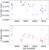 |
Fig. 1 Time series of the SMW (upper panel) and H-α (lower panel) spectroscopic activity indices derived from the ESPRESSO spectra. |
Summary of the RVs analysed in this work.
4.2 Combined analysis
We performed a combined light curve+RV fit using nightly binned RVs for HARPS, CORALIE, and ESPRESSO in order to average out short-term stellar jitter (e.g. p-modes and granulation). The analysis was carried out using the code presented in Demangeon et al. (2018). It combines parts of the Python packages RADVEL (Fulton et al. 2018) (RADVEL.KEPLER.RV_DRIVE), for the RVs, and BATMAN (Kreidberg 2015), for the photometry, into a Bayesian framework to compute the posterior probability of the planetary model parameters. This posterior function is then maximized using first the Nelder-Mead simplex algorithm implemented in the Python package scipy.optimize (Gao & Han 2012); this is followed by an exploration with the affine-invariant ensemble sampler MCMC algorithm, implemented by the Python package EMCEE (Foreman-Mackey et al. 2013).
As done by Gandolfi et al. (2018) and Huang et al. (2018), we modelled any additional source of noise in the RVs not included in the nominal σRV(t) by simply fitting uncorrelated jitter terms added in quadrature to σRV(t). We did not find evidence in the TESS light curve, RVs, or spectroscopic activity diagnostics of a signal modulated over the stellar rotational period ~18 d, as was found by Zurlo et al. (2018), or its harmonics that would justify the use of a more sophisticated model to mitigate thestellar activity (e.g. Gaussian process regression). To this regard, based on our measurements of vsin i⋆ and R⋆, we estimated the upper limit of the rotation period of π Men to be 17.7 ± 0.5 d. We tested models with the eccentricity ec of π Men c set to zero or fitted as a free parameter to explore if the use of ESPRESSO RVs and additional TESS transits helps to constrain ec. This parameter was not well determined by Huang et al. (2018) and Gandolfi et al. (2018), who could constrain ec to be less than 0.3 and 0.45 (at 68% of confidence), respectively.
The results of our analysis and those from the literature are summarized in Table 3. Based on the Bayesian information criterion (BIC), we find that the model with a fixed circular orbit is strongly favoured (BICecc–BICcirc > 10), and we adopted it as our final solution. However, we cannot rule out a mild eccentricity (the posterior is not a zero-mean Gaussian distribution), and we are able to set the upper limit of ec < 0.21 (corresponding to the 68th percentile of the posterior), providing a further constraint for studies of the dynamical interaction with the massive and eccentric companion b. The best-fit model for the transit light curve of π Men c (i.e. that obtained using the derived median values for the free parameters) is shown in Fig. 2, with the 22 individual transits we analysed combined. Figure 3 shows the best-fit spectroscopic orbits for planets b and c. The mass of π Men c mc = 4.3 ± 0.7 M⊕ is measured with a precision of ~16%.
The upper panel of Fig. 4 shows the GLS periodogram of the ESPRESSO RV residuals, after removing the signal induced by planet b. It clearly shows the dominant peak at the orbital period of π Men c, with a bootstrapping false alarm probability (FAP) of 0.6% determined from 10 000 simulated datasets. The dispersion of the ESPRESSO residuals is 1.2 m s−1 (middle panel of Fig. 4), half the root mean square (RMS) of the HARPS residuals. The uncorrelated jitter term σjitter, ESPRESSO ~ 1.2 m s−1 and the RMS of the residuals are one order of magnitude higher that the typical RV precision; this could be due to effects of the stellar magnetic activity, for which our model does not include an analytic term. We then considered the ESPRESSO residuals obtained after also removing the signal of π Men c; we did not find significant correlations with the BIS, the SMW, or H-α activity diagnostics. Therefore, explaining the observed “excess” of jitter in terms of activity does not appear straightforward. The GLS periodogram of these residuals is shown in the last panel of Fig. 4. Through a bootstrap (with replacement) analysis, we find that the peak with the highest power has an FAP of ~37%. We further discuss this signal in Appendix C.
The ESPRESSO and CORALIE observations cover the periastron passage of planet b (Tb, peri = 2458388.6 ± 2.2 BJD), allowing for a more precise determination of the Doppler semi-amplitude Kb and eccentricity eb. With 18 additional transits of π Men c available, we improved the accuracy and precision of the transit ephemeris and of the transit depth, which, in combination with the re-determined stellar radius, resulted in a planet radius Rc = 2.11 ± 0.05 R⊕, slightly larger than that reported in the literature.
According to our results, the predicted time of inferior conjunction Tb, conj of the outermost companion falls within the time span of the TESS observations (sector 12). We checked the light curve within a ± 5σ range from the best-fit value (Fig. 5) and did not find evidence for the transit of π Men b. Assuming a radius of 0.8 RJup for π Men b (Sorahana et al. 2013), we could detect transits of the sub-stellar companion if the orbital inclination angle ib were within the penumbra cone defined by the narrow angle ±~0.1 deg as measured from a perfectly edge-on orbit.
Best-fit results of the π Men photometry+RV joint modelling.
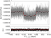 |
Fig. 2 Transit signal of π Men c observed in the TESS light curve. Data from 22 individual transits are phase-folded to the orbital period of the planet, and the red curve represents the best-fit model (Table 3). |
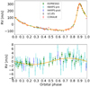 |
Fig. 3 Spectroscopic orbits of the two planets in the π Men system (upper panel: π Men b; lower panel: π Men c; best-fit solutions in Table 3). The orange curve represents the best-fit model. For π Men c, we do not show the more scattered and less precise UCLES and CORALIE data for a bettervisualization, and the error bars include uncorrelated jitters added in quadrature to σRV. |
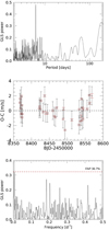 |
Fig. 4 Upper panel: GLS periodogram of the ESPRESSO RV residuals, after removing the best-fit Doppler signal of π Men b. We assumed RV error bars with the uncorrelated jitter added in quadrature to the formal σRV. The highest peak occurs at the orbital period of π Men c, with a bootstrapping FAP of 0.6% determined from 10 000 simulated datasets. Middle panel: ESPRESSO RV residuals after removing the adopted two-planet model solution in Table 3. The error bars in black include the uncorrelated jitter derived from our analysis, which has been added in quadrature to the σRV uncertainties (indicated in red). Lower panel: GLS periodogram of the ESPRESSO residuals, with the RV error bars including the uncorrelated jitter added in quadrature to the formal σRV. The FAP of the main peak at ~190 d was determined through a bootstrap (with replacement) analysis using 10 000 simulated datasets. This signal is further discussed in Appendix C. |
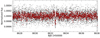 |
Fig. 5 Portion of the TESS light curve centred around the predicted time of inferior conjunction of π Men b (± 5σ). Red dots represent averages of five-data point bins. The only visible transit signal is that of π Men c. |
4.3 Mass limits for co-orbital companions to π Men c
Given the high precision of the ESPRESSO and HARPS RVs, we explored the possibility of the presence of co-orbital bodies to π Men c through the technique described in Leleu et al. (2017) and subsequently applied by Lillo-Box et al. (2018a,b). This technique uses the information from the transit time of the planet and the full RV dataset to constrain the time lag between theplanet transit and the time of zero RV (a generalization of the Ford & Gaudi 2006 methodology). The technique is based on modelling the RV data by using Eq. (18) from Leleu et al. (2017), where the key parameter α contains all the information about the co-orbital signal. A posterior distribution of α compatible with zero discards the presence of co-orbitals up to a certain mass. Contrarily, if α is significantly different from zero, the data contain hints for the presence of a co-orbital body, with negative values corresponding to L4 and positive values to L5. In this framework, we analysed the RV dataset with such a model using the EMCEE Markov chain Monte Carlo (MCMC) ensemble sampler to explore the parameter space. We used the same priors for the parameters in common with the analysis presented in Sect. 4.2 and a uniform prior  for the α parameter. We used 96 random walkers and 10 000 steps per walker with two first burn-in chains and a final production chain with 5000 steps. We checked the convergence of the chains by estimating the autocorrelation times and checking that the chain length was at least 30 times this autocorrelation time for all parameters. The result provides a value for the α parameter of
 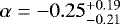 . Although shifted towards negative values, the posterior distribution is compatible with zero at the 95% confidence level. Consequently, we cannot confirm the presence of co-orbitals. However, given this posterior value, we can certainly put upper limits to the presence of co-orbitals at both Lagrangian points. By using the 95% confidence levels, we can discard co-orbitals more massive than 3.1 M⊕ at L4 and 0.3 M⊕ at L5 (i.e. co-orbitals more massive than three times the mass of Mars at L5). An intensive and dedicated effort with additional RV data would then be needed to further explore the L4 region.
5 Constraining the relative alignment of the planetary orbital planes
We further constrained the relative alignment of the orbital planes of the two planets using a combination of the high-precision spectroscopic orbit for π Men b, obtained thanks to the contribution of the ESPRESSO dataset, and the absolute astrometry of HIPPARCOS and Gaia, as follows. We first took the cross-calibrated HIPPARCOS and Gaia DR2 π Men propermotion values and the scaled HIPPARCOS-Gaia positional difference from the Brandt (2018, 2019)3 catalogue of astrometric accelerations. The latter quantity is defined as the difference in astrometric position between the two catalogues divided by the corresponding ~25-yr time baseline, a factor of ~4.4 longer than the orbital period of π Men b. It corresponds to a long-term proper motion vector that can be considered as a close representation of the tangential velocity of the barycentre of the system. By subtracting this long-term proper motion from the quasi-instantaneous proper motions of the two catalogues, one obtains a pair of “proper motion difference”, “astrometric acceleration”, or “proper motion anomaly” values (i.e. Δμ), which are assumedto entirely describe the projected velocity of the photocentre around the barycentre at the HIPPARCOS and Gaia DR2 epochs4. The observed Δμ values (see Table 4) contain information on the orbital motion of π Men b (the orbital effect due to π Men c is entirely negligible). We elected to use the π Men proper motion vector from the Brandt (2018, 2019) catalogue instead of the physically equivalent and equally well-validated quantity in the catalogue produced by Kervella et al. (2019) for two reasons: (a) the former catalogue is constructed based on a linear combination of the two HIPPARCOS reductions, a choice that appears preferable with respect to considering either reduction individually; (b) Brandt (2018, 2019) brings the composite HIPPARCOS astrometry on the bright reference frame of Gaia DR2, resulting in an updated error model with rather conservativeuncertainties, which are shown to be statistically well-behaved. The robustness of the Brandt (2018, 2019) catalogue has recently been further probed by Lindegren (2020a,b), who compare the spin and orientation of the bright reference frame of Gaia DR2 using very long baseline interferometry observations of radio stars and the independent assessment of the rotation made by Brandt (2018, 2019).
We then followed Kervella et al. (2020) and explored, via an MCMC algorithm, the ranges of inclination ib and the longitude of the ascending node Ωb compatible with the absolute astrometry and the spectroscopically determined orbital parameters (and their uncertainties). The values of ib and Ωb (using uniform priors on cos ib and Ωb over the allowed ranges for both prograde and retrograde motion) are fitted in a model of the proper motion differences that we built by averaging over the actual HIPPARCOS and Gaia observing windows, adopting the times of HIPPARCOS observations available in the HIPPARCOS-2 catalogue (van Leeuwen 2007), and taking the Gaia transit times from the Gaia Observation Forecast Tool (GOST)5. This allowed us to cope with the “smearing” effect of the orbital motion thanks to the fact that the observed Δμ values are time averages of the intrinsic velocity vector of the star over the HIPPARCOS and Gaia observing periods. For π Men b, this effect isnon-negligible (see Kervella et al. 2019).
The orbital fit results to the HIPPARCOS and Gaia absolute astrometry are reported in Table 4, while in Fig. D.1 we show the posterior distributions for the model parameters explored in our MCMC analysis. The corresponding inferred true mass of π Men b is mb =14.1 MJup. Furthermore, the evidence for orbital motion at both the HIPPARCOS and Gaia epochs also allows us to break the degeneracy between prograde and retrograde motion, the latter being clearly favoured. Overall, one would infer a highly significant non-coplanarity between π Men b and π Men c. Given that the inclination of the orbital plane of the latter is known, we can then directly provide constraints on the possible range of mutual inclination angles irel, expressed as a function of the unknown longitude of the ascending node of π Men c (allowed to vary in the range [0,360] deg). The results are shown in Fig. D.2. We find that 52.3 ≤ irel ≤ 128.8 deg, at the 1σ-level. The irel distribution shows two clear peaks at 50 deg and 130 (=180–50) deg. A sketch of the 3D system’s architecture is given in Fig. 6.
Components of the proper motion vector difference for π Men, priors, and best-fit results for the MCMC analysis of the Δμ time series constrained by the spectroscopic orbital solution.
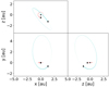 |
Fig. 6 Sketch of the planets’ orbits in Jacobi coordinates, showing the 3D architecture of the π Men system. Theorbits are not to scale: that of planet c has been enlarged to better show the mutual inclinations between the planetary orbital planes. |
6 Summary and discussion
One main goal of our study was to assess the performance of a very-high-precision RV follow-up of a bright planet-hosting star with the ESPRESSO spectrograph, and the characterization of the low-mass transiting planet π Men c came as an ideal test case. The multi-planetsystem orbiting π Men was the object of recent characterization studies using space-based photometry and high-precision RVs, such as those collected with HARPS; therefore, our results can be compared with those in the literature. Figure 3 (lower panel) shows the low dispersion of the ESPRESSO RV measurement around the best-fit spectroscopic orbit of π Men c. After removing the best-fit Keplerian of the companion π Men b and the offsets of the pre- and post-technical intervention, we modelled the residuals of the ESPRESSO RVs with a Keplerian function to quantify how well the orbit of planet c is fitted using only this dataset. This Monte Carlo analysis wasperformed using the open source Bayesian inference tool MULTINEST v3.10 (e.g. Feroz et al. 2019), through the PYMULTINEST python wrapper (Buchner et al. 2014). We obtained the Doppler semi-amplitude Kc = 1.5 ± 0.3 m s−1, which has basically the same precision as the value we obtained using the RVs from all the instruments. This result, based on data collected on 37 nights over a time span of 200 days, does a good job of illustrating the performance reached by ESPRESSO on such a target. From these residuals, we derived upper limits to the minimum mass of planets that may still be undetected as a function their orbital period. The detection limits are calculated by injecting trial circular orbits into the observed data (e.g. Cumming et al. 1999). We explored orbital periods from 0.5 days to twice the time span of the ESPRESSO data, and semi-amplitudes up to 10 km s−1 (using a binary search). For ten linearly spaced phases, the periodogram power at the injected period is compared with the 1% FAP level in the original residuals. If, for all phases, the former is higher, the injected planet is considered detected. Using our measured stellar mass, the semi-amplitudes are converted to the minimum mass of the planet. The detection limits are shown in Fig. 7, from which we can conclude that undetected companions to π Men within the orbit of π Men c should have a minimum mass lower than ~2 M⊕. We can exclude planets with minimum masses less than ~10 M⊕ and with orbital periods greater than 100 days.
Our analysis of HD 39091, based on spectroscopy and photometry, was enhanced by the use of astrometry; this allowed for a much more complete characterization of the system’s properties and architecture. The evidence for a large mutual inclination between π Men b and c naturally raises the possibility of strong secular dynamical perturbations on the inner planet’s orbital arrangement. In the co-planar case, the amplitude of transit timing variations (TTVs) for π Men c is not expected to exceed a few tens of seconds (e.g. Holman & Murray 2005). No clear departure from a linear ephemeris is detected within the error bars in the residuals of the time of transit centre (Fig. 8). We used TTVFAST (Deck et al. 2014) to explore whether the high mutual inclination might induce a detectable signal, also given the fact that the periastron passage of π Men b occurred within the time span of the TESS observations. However, the analysis with TTVFAST, limited to the time span of the TESS observations, did not produce any detectable TTV signal and was in agreement with our observations, resulting in the longitude of the ascending node of π Men c being fully unconstrained. This is not surprising given the fact that only a small fraction of the full orbit of the perturber has been covered, a circumstance that could prevent the recovery of a TTV signal (Deck et al. 2014).
The high value of irel could in principle cause significant secular evolution in the eccentricity and inclination of π Men c (see e.g. Kozai 1962; Lidov 1962; Holman et al. 1997), with the effect of possibly shifting the planet out from the transiting configuration observed today. The system’s architecture is also suggestive of a violent dynamical evolution history, which mightpoint to a high-eccentricity migration scenario and a significant degree of spin-orbit misalignment of the transiting inner planet (see e.g. Fabrycky & Tremaine 2007; Chatterjee et al. 2008; Ogilvie 2014; Hamers et al. 2017).
Based on the deuterium burning-mass limit for separating planets and brown dwarfs, which is theoretically established at ~13 MJup for solar metallicity and the cosmic abundance of deuterium (Burrows et al. 1995; Saumon et al. 1996; Chabrier et al. 2000), π Men b should be classified as a brown dwarf. Brown dwarf companions to a main sequence star appear to be very rare in close orbits (<3 AU), and their occurrence rate is much lower than for giant planets and stars. For instance, Grether & Lineweaver (2006) found that while ~16% of Sun-like stars have close companions (orbital period <5 yr) more massive than Jupiter, only <1% are brown dwarfs, whereas 11 and 5% are stars and giant planets, respectively. This paucity is traditionally refereed to as the “brown dwarf desert”. Today, the Kepler–K2 and TESS missions and the superWASP survey have proved that this desert is not as “dry” as originally thought. Several brown dwarfs have been detected with short orbital periods (see e.g. Carmichael et al. 2019, 2020; Persson et al. 2019; Šubjak et al. 2020; Parviainen et al. 2020), and their occurrence rate has been revised to 2.0 ± 0.5% by Kiefer et al. (2019). Our precise mass determination for π Men b contributes to further populate the brown dwarf desert.
The results of our study, based on multi-technique observations, make π Men a benchmark multi-body system – with a brown dwarf cohabiting with a super-Earth around a solar-like star – for which the 3-D architecture has been unveiled with precision. This indeed encourages further follow-up and detailed modelling of the π Men planetary system to understand its formation and evolution. We note that the nominal schedule of future TESS observations available at the moment includes the field of π Men for six more sectors in 2020–2021. The new data could be used to further constrain the TTVs of planet c.
Note. A few days before the formal acceptance of this paper, an independent study about the architecture of the π Men planetary system was published (Xuan & Wyatt 2020). The results of that work, based on public data and not including the ESPRESSO observations, confirm the high mutual inclination of the orbital planes of π Men b and c. Our results are in agreement with those of Xuan & Wyatt (2020) and are characterized by a better formal precision.
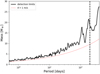 |
Fig. 7 Detection limits for additional planetary companions in the π Men system. The dashed red curve corresponds to a Doppler signal with a semi-amplitude of 1 m s−1, and the vertical dashed line marks the location of the time span of the ESPRESSO data. |
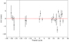 |
Fig. 8 Transit timing variations measured from the TESS light curve. The dashed vertical line shows the epoch of the periastron passage of π Men b. |
Acknowledgements
We thank the referee Pierre Kervella for his comments that improved the contents of this work. M.D. acknowledges financial support from Progetto Premiale 2015 FRONTIERA (OB.FU. 1.05.06.11) funding scheme of the Italian Ministry of Education, University, and Research, and also acknowledge the computing centres of INAF – Osservatorio Astronomico di Trieste/Osservatorio Astrofisico di Catania, under the coordination of the CHIPP project, for the availability of computing resources and support. C.L. and F.P. would like to acknowledge the Swiss National Science Foundation (SNSF) for supporting research with ESPRESSO through the SNSF grants nr. 140649, 152721, 166227 and 184618. The ESPRESSO Instrument Project was partially funded through SNSF’s FLARE Programme for large infrastructures. This work has been carriedout in part within the framework of the NCCR PlanetS supported by the Swiss National Science Foundation. This work was supported by FCT – Fundação para a Ciência e a Tecnologia through national funds and by FEDER through COMPETE2020 – Programa Operacional Competitividade e Internacionalização by these grants: UID/FIS/04434/2019; UIDB/04434/2020; UIDP/04434/2020; PTDC/FIS-AST/32113/2017 & POCI-01-0145-FEDER-032113; PTDC/FIS-AST/28953/2017 & POCI-01-0145-FEDER-028953; PTDC/ FIS-AST/28987/2017 & POCI-01-0145-FEDER-028987. S.C.C.B., V.Z.A., S.G.S. and J.P.S.F. acknowledge support from FCT through FCT contracts nr. IF/01312/2014/CP1215/CT0004, IF/00650/2015/CP1273/CT0001, IF/00028/ 2014/CP1215/CT0002, DL 57/2016/CP1364/CT0005. O.D.S.D. is supported in the form of work contract (DL 57/2016/CP1364/CT0004) funded by national funds through Funda cão para a Ciência e Tecnologia (FCT). J.L.-B. has been funded by the Spanish State Research Agency (AEI) Projects No.ESP2017-87676-C5-1-R and No. MDM-2017-0737 Unidad de Excelencia “María de Maeztu”– Centro de Astrobiología (INTA-CSIC). J.P.F. is supported in the form of a work contract funded by national funds through FCT with reference DL57/2016/CP1364/CT0005. V.B. acknowledges support by the Swiss National Science Foundation (SNSF) in the frame of the National Centre for Competence in Research “PlanetS”. This project has received funding from the European Research Council (ERC) under the European Union’s Horizon 2020 research and innovation programme (project Four Aces, grant agreement No 724427). R.R., C.A.P., J.I.G.H., A.S.M., and M.R.Z.O. acknowledge financial support from the Spanish Ministry of Science and Innovation (MICINN) projects AYA2017-86389-P and AYA2016-79425-C3-2-P. J.I.G.H. acknowledges financial support from the Spanish MICINN under the 2013 Ramón y Cajal program RYC-2013-14875. M.T.M. thanks the Australian Research Council for Future Fellowship grant FT180100194 which supported this work. Partial financial support from the agreement ASI-INAF n.2018-16-HH.0 is gratefully acknowledgded. This work has made use of data from the European Space Agency (ESA) mission Gaia (https://www.cosmos.esa.int/gaia), processed by the Gaia Data Processing and Analysis Consortium (DPAC, https://www.cosmos.esa.int/web/gaia/dpac/consortium). Funding for the DPAC has been provided by national institutions, in particular the institutions participating in the Gaia Multilateral Agreement. This publication makes use of The Data & Analysis Center for Exoplanets (DACE), which is a facility based at the University of Geneva (CH) dedicated to extrasolar planets data visualization, exchange and analysis. DACE is a platform of the Swiss National Centre of Competence in Research (NCCR) PlanetS, federating the expertise in Exoplanet research. The DACE platform is available at https://dace.unige.ch.
Appendix A: Co-added ESPRESSO spectrum
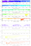 |
Fig. A.1 Upper plot: co-added, normalized, merged, and RV-corrected ESPRESSO spectrum of π Men using the starII DAS workflow in a subset of 40 ESPRESSO spectra. Lower plot: selected regions of the spectrum to illustrate its quality. |
Appendix B: ESPRESSO and CORALIE data
The RVs and activity diagnostics used in this work are listed in Tables B.1 and B.26.
Appendix C: Further analysis of the ESPRESSO RV residuals
As discussed in Sect. 4.2, the GLS periodogram of the two-planet model RV residuals shows a peak at ~190 d (last panel of Fig. 4). Even though it appears insignificant according to a bootstrap analysis, we nonetheless investigated the properties of this signal in more detail by performing a Monte Carlo analysis with MULTINEST and a Bayesian model comparison. To this purpose, we considered the ESPRESSO RV residuals after subtracting the best-fit spectroscopic orbit of π Men b and instrumental offsets; we modelled them with two Keplerians, setting their eccentricities to zero (one for the Doppler signal due to π Men c) and using uninformative priors for the semi-amplitude, period, and time of the inferior conjunction of the other Doppler signal ( m s−1;
 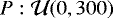 d;
d;  BJD). We find that the fit improves with respect to only including π Men c (see Sect. 6). The Bayesian factor is ~ + 5, favouring the model with two signals, with the semi-amplitude of planet c Kc = 1.3 ± 0.2 m s−1, slightly lower and more significant than Kc = 1.5 ± 0.3 m s−1; the uncorrelated jitter of the post-intervention data slightly decreases to 1.0
 m s−1. For the second signal, we find
 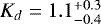 m s−1 and
  d. The posterior distributions for the free model parameters are shown in Fig. C.1, and the best-fit model for the additional signal is shown in Fig. C.2. If it is due to a third planet in the system, this signal would correspond to a minimum mass of ~10 M⊕. The results of our analysis are not sufficiently robust to reach any clear conclusion about the nature of this signal that appears in the ESPRESSO data, and we did not perform any dynamical analysis to verify the orbital stability. Further spectroscopic follow-up is indeed required to confirm the signal and improve the phase coverage.
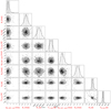 |
Fig. C.1 Posterior distributions for the free parameters of the two-planet model tested on the RV ESPRESSO residuals, after removing the spectroscopic orbit of π Men b and instrumental offsets from the original dataset. |
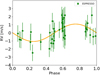 |
Fig. C.2 Best-fit model (orange curve) for the additional ~190-d signal found in the RV residuals of ESPRESSO, as derived with a Monte Carlo analysis. The error bars include a constant jitter term added in quadrature to the formal RV uncertainties. |
Appendix D: Radial velocity and astrometric joint analysis
Figure D.1 shows the posterior distributions for ib and Ωb derived from the analysis described in Sect. 5. As one can see, the orbital plane inclination angle ib and the longitude of the ascending node Ωb for planet b are both fitted with high formal precision:  deg and
 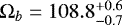 deg. Figure D.2 shows the distribution of the mutual inclination angles irel between the companions b and c to π Men.
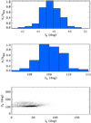 |
Fig. D.1 Topand central panels: posterior distributions for ib and Ωb. Lower panel: joint posterior distributions for the two model parameters. |
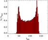 |
Fig. D.2 Distribution of possible mutual inclinations between π Men b and c. |
References
- Barros, S. C. C., Demangeon, O., & Deleuil, M. 2016, A&A, 594, A100 [NASA ADS] [CrossRef] [EDP Sciences] [Google Scholar]
- Batalha, N. E., Lewis, T., Fortney, J. J., et al. 2019, ApJ, 885, L25 [Google Scholar]
- Brandt, T. D. 2018, ApJS, 239, 31 [NASA ADS] [CrossRef] [Google Scholar]
- Brandt, T. D. 2019, ApJS, 241, 39 [NASA ADS] [CrossRef] [Google Scholar]
- Brandt, T. D., Dupuy, T. J., & Bowler, B. P. 2019, AJ, 158, 140 [NASA ADS] [CrossRef] [Google Scholar]
- Buchner, J., Georgakakis, A., Nandra, K., et al. 2014, A&A, 564, A125 [NASA ADS] [CrossRef] [EDP Sciences] [Google Scholar]
- Burrows, A., Saumon, D., Guillot, T., Hubbard, W. B., & Lunine, J. I. 1995, Nature, 375, 299 [NASA ADS] [CrossRef] [Google Scholar]
- Calissendorff, P., & Janson, M. 2018, A&A, 615, A149 [NASA ADS] [CrossRef] [EDP Sciences] [Google Scholar]
- Carmichael, T. W., Latham, D. W., & Vand erburg, A. M. 2019, AJ, 158, 38 [NASA ADS] [CrossRef] [Google Scholar]
- Carmichael, T. W., Quinn, S. N., Mustill, A. e. J., et al. 2020, AJ, 160, 53 [Google Scholar]
- Chabrier, G., Baraffe, I., Allard, F., & Hauschildt, P. 2000, ApJ, 542, L119 [CrossRef] [Google Scholar]
- Chatterjee, S., Ford, E. B., Matsumura, S., & Rasio, F. A. 2008, ApJ, 686, 580 [NASA ADS] [CrossRef] [Google Scholar]
- Cumming, A., Marcy, G. W., & Butler, R. P. 1999, ApJ, 526, 890 [NASA ADS] [CrossRef] [Google Scholar]
- da Silva, L., Girardi, L., Pasquini, L., et al. 2006, A&A, 458, 609 [NASA ADS] [CrossRef] [EDP Sciences] [Google Scholar]
- Deck, K. M., Agol, E., Holman, M. J., & Nesvorný, D. 2014, ApJ, 787, 132 [CrossRef] [Google Scholar]
- Delgado Mena, E., Bertrán de Lis, S., Adibekyan, V. Z., et al. 2015, A&A, 576, A69 [NASA ADS] [CrossRef] [EDP Sciences] [Google Scholar]
- Demangeon, O. D. S., Faedi, F., Hébrard, G., et al. 2018, A&A, 610, A63 [CrossRef] [EDP Sciences] [Google Scholar]
- Di Marcantonio, P., Sosnowska, D., Cupani, G., et al. 2018, SPIE Conf. Ser., 10704, 107040F [Google Scholar]
- Doyle, A. P., Davies, G. R., Smalley, B., Chaplin, W. J., & Elsworth, Y. 2014, MNRAS, 444, 3592 [NASA ADS] [CrossRef] [Google Scholar]
- Dupuy, T. J., Brandt, T. D., Kratter, K. M., & Bowler, B. P. 2019, ApJ, 871, L4 [NASA ADS] [CrossRef] [Google Scholar]
- Fabrycky, D., & Tremaine, S. 2007, ApJ, 669, 1298 [NASA ADS] [CrossRef] [Google Scholar]
- Feng, F., Anglada-Escudé, G., Tuomi, M., et al. 2019, MNRAS, 490, 5002 [NASA ADS] [CrossRef] [Google Scholar]
- Feroz, F., Hobson, M. P., Cameron, E., & Pettitt, A. N. 2019, Open J. Astrophys., 2, 10 [Google Scholar]
- Ford, E. B., & Gaudi, B. S. 2006, ApJ, 652, L137 [NASA ADS] [CrossRef] [Google Scholar]
- Foreman-Mackey, D., Hogg, D. W., Lang, D., & Goodman, J. 2013, PASP, 125, 306 [CrossRef] [Google Scholar]
- Fulton, B. J., Petigura, E. A., Blunt, S., & Sinukoff, E. 2018, PASP, 130, 044504 [NASA ADS] [CrossRef] [Google Scholar]
- Gaia Collaboration (Brown, A. G. A., et al.) 2018, A&A, 616, A1 [NASA ADS] [CrossRef] [EDP Sciences] [Google Scholar]
- Gandolfi, D., Barragán, O., Livingston, J. H., et al. 2018, A&A, 619, L10 [NASA ADS] [CrossRef] [EDP Sciences] [Google Scholar]
- Gao, F., & Han, L. 2012, Comput. Optim. Appl., 51, 259 [CrossRef] [Google Scholar]
- García Muñoz, A., Youngblood, A., Fossati, L., et al. 2020, ApJ, 888, L21 [NASA ADS] [CrossRef] [Google Scholar]
- Grandjean, A., Lagrange, A. M., Beust, H., et al. 2019, A&A, 627, L9 [NASA ADS] [CrossRef] [EDP Sciences] [Google Scholar]
- Grether, D., & Lineweaver, C. H. 2006, ApJ, 640, 1051 [NASA ADS] [CrossRef] [Google Scholar]
- Hamers, A. S., Antonini, F., Lithwick, Y., Perets, H. B., & Portegies Zwart, S. F. 2017, MNRAS, 464, 688 [NASA ADS] [CrossRef] [Google Scholar]
- Holman, M. J., & Murray, N. W. 2005, Science, 307, 1288 [NASA ADS] [CrossRef] [PubMed] [Google Scholar]
- Holman, M., Touma, J., & Tremaine, S. 1997, Nature, 386, 254 [NASA ADS] [CrossRef] [Google Scholar]
- Huang, C. X., Burt, J., Vanderburg, A., et al. 2018, ApJ, 868, L39 [NASA ADS] [CrossRef] [Google Scholar]
- Jones, H. R. A., Paul Butler, R., Tinney, C. G., et al. 2002, MNRAS, 333, 871 [NASA ADS] [CrossRef] [Google Scholar]
- Kervella, P., Arenou, F., Mignard, F., & Thévenin, F. 2019, A&A, 623, A72 [NASA ADS] [CrossRef] [EDP Sciences] [Google Scholar]
- Kervella, P., Arenou, F., & Schneider, J. 2020, A&A, 635, L14 [CrossRef] [EDP Sciences] [Google Scholar]
- Kiefer, F., Hébrard, G., Sahlmann, J., et al. 2019, A&A, 631, A125 [NASA ADS] [CrossRef] [EDP Sciences] [Google Scholar]
- King, G. W., Wheatley, P. J., Bourrier, V., & Ehrenreich, D. 2019, MNRAS, 484, L49 [NASA ADS] [CrossRef] [Google Scholar]
- Kozai, Y. 1962, AJ, 67, 591 [Google Scholar]
- Kreidberg, L. 2015, PASP, 127, 1161 [NASA ADS] [CrossRef] [Google Scholar]
- Kurucz, R. 1993, ATLAS9 Stellar Atmosphere Programs and 2 km/s grid. Kurucz CD-ROM No. 13. Cambridge, 13 [Google Scholar]
- Leleu, A., Robutel, P., Correia, A. C. M., & Lillo-Box, J. 2017, A&A, 599, L7 [NASA ADS] [CrossRef] [EDP Sciences] [Google Scholar]
- Lidov, M. L. 1962, Planet. Space Sci., 9, 719 [NASA ADS] [CrossRef] [Google Scholar]
- Lillo-Box, J., Barrado, D., Figueira, P., et al. 2018a, A&A, 609, A96 [NASA ADS] [CrossRef] [EDP Sciences] [Google Scholar]
- Lillo-Box, J., Leleu, A., Parviainen, H., et al. 2018b, A&A, 618, A42 [NASA ADS] [CrossRef] [EDP Sciences] [Google Scholar]
- Lindegren, L. 2020a, A&A, 633, A1 [NASA ADS] [CrossRef] [EDP Sciences] [Google Scholar]
- Lindegren, L. 2020b, A&A, 637, C5 [CrossRef] [EDP Sciences] [Google Scholar]
- Ogilvie, G. I. 2014, ARA&A, 52, 171 [Google Scholar]
- Parviainen, H., Palle, E., Zapatero-Osorio, M. R., et al. 2020, A&A, 633, A28 [NASA ADS] [CrossRef] [EDP Sciences] [Google Scholar]
- Pepe, F., Cristiani, S., Rebolo, R., et al. 2020, A&A, submitted [Google Scholar]
- Persson, C. M., Csizmadia, S., Mustill, A. e. J., et al. 2019, A&A, 628, A64 [NASA ADS] [CrossRef] [EDP Sciences] [Google Scholar]
- Ricker, G. R., Winn, J. N., Vanderspek, R., et al. 2015, J. Astron. Telesc. Instrum., Syst., 1, 014003 [Google Scholar]
- Rodrigues, T. S., Girardi, L., Miglio, A., et al. 2014, MNRAS, 445, 2758 [NASA ADS] [CrossRef] [Google Scholar]
- Rodrigues, T. S., Bossini, D., Miglio, A., et al. 2017, MNRAS, 467, 1433 [NASA ADS] [Google Scholar]
- Santos, N., Sousa, S. G., Mortier, A., et al. 2013, A&A, 556, A150 [NASA ADS] [CrossRef] [EDP Sciences] [Google Scholar]
- Saumon, D., Hubbard, W. B., Burrows, A., et al. 1996, ApJ, 460, 993 [NASA ADS] [CrossRef] [Google Scholar]
- Ségransan, D., Delisle, J.-B., Dumusque, X., et al. 2020, A&A, submitted [Google Scholar]
- Sneden, C. A. 1973, PhD thesis, The University of Texas at Austin, TX, USA [Google Scholar]
- Snellen, I. A. G., & Brown, A. G. A. 2018, Nat. Astron., 2, 883 [NASA ADS] [CrossRef] [Google Scholar]
- Sorahana, S., Yamamura, I., & Murakami, H. 2013, ApJ, 767, 77 [NASA ADS] [CrossRef] [Google Scholar]
- Sousa, S. G. 2014, Determination of Atmospheric Parameters of B-, A-, F- and G-Type Stars (Cham: Springer), 297 [Google Scholar]
- Sousa, S. G., Santos, N. C., Israelian, G., Mayor, M., & Monteiro, M. J. P. F. G. 2007, A&A, 469, 783 [NASA ADS] [CrossRef] [EDP Sciences] [Google Scholar]
- Sousa, S. G., Santos, N. C., Mayor, M., et al. 2008, A&A, 487, 373 [NASA ADS] [CrossRef] [EDP Sciences] [MathSciNet] [Google Scholar]
- Sousa, S. G., Santos, N. C., Israelian, G., et al. 2011, A&A, 526, A99 [NASA ADS] [CrossRef] [EDP Sciences] [Google Scholar]
- Sousa, S. G., Santos, N. C., Adibekyan, V., Delgado-Mena, E., & Israelian, G. 2015, A&A, 577, A67 [NASA ADS] [CrossRef] [EDP Sciences] [Google Scholar]
- Sousa, S. G., Adibekyan, V., Delgado-Mena, E., et al. 2018, A&A, 620, A58 [NASA ADS] [CrossRef] [EDP Sciences] [Google Scholar]
- Šubjak, J., Sharma, R., Carmichael, T. W., et al. 2020, AJ, 159, 151 [CrossRef] [Google Scholar]
- Tsantaki, M., Andreasen, D. T., Teixeira, G. D. C., et al. 2017, MNRAS, 473, 5066 [NASA ADS] [CrossRef] [Google Scholar]
- Udry, S., Mayor, M., Naef, D., et al. 2000, A&A, 356, 590 [NASA ADS] [Google Scholar]
- van Leeuwen, F. 2007, A&A, 474, 653 [NASA ADS] [CrossRef] [EDP Sciences] [Google Scholar]
- Xuan, J. W., & Wyatt, M. C. 2020, MNRAS, 497, 2096 [Google Scholar]
- Zechmeister, M., & Kürster, M., 2009, A&A, 496, 577 [NASA ADS] [CrossRef] [EDP Sciences] [Google Scholar]
- Zurlo, A., Mesa, D., Desidera, S., et al. 2018, MNRAS, 480, 35 [NASA ADS] [CrossRef] [Google Scholar]
The original catalogue presented in Brandt (2018) is superseded by the new version published in Brandt (2019), which corrects an error in the calculation of the perspective acceleration in right ascention.
For recent applications of this technique for the detection of stellar and sub-stellar companions, see e.g. Calissendorff & Janson 2018; Snellen & Brown 2018; Kervella et al. 2019; Brandt et al. 2019; Dupuy et al. 2019; Feng et al. 2019; Grandjean et al. 2019.
The data are also made publicly available via the DACE platform, available at the website https://dace.unige.ch/radialVelocities/?pattern=Pi%20Men and via the python API’s website https://dace.unige.ch/radialVelocities/?pattern=Pi%20Men.
All Tables
Components of the proper motion vector difference for π Men, priors, and best-fit results for the MCMC analysis of the Δμ time series constrained by the spectroscopic orbital solution.
All Figures
|
Fig. 1 Time series of the SMW (upper panel) and H-α (lower panel) spectroscopic activity indices derived from the ESPRESSO spectra. |
| In the text | |
|
Fig. 2 Transit signal of π Men c observed in the TESS light curve. Data from 22 individual transits are phase-folded to the orbital period of the planet, and the red curve represents the best-fit model (Table 3). |
| In the text | |
|
Fig. 3 Spectroscopic orbits of the two planets in the π Men system (upper panel: π Men b; lower panel: π Men c; best-fit solutions in Table 3). The orange curve represents the best-fit model. For π Men c, we do not show the more scattered and less precise UCLES and CORALIE data for a bettervisualization, and the error bars include uncorrelated jitters added in quadrature to σRV. |
| In the text | |
|
Fig. 4 Upper panel: GLS periodogram of the ESPRESSO RV residuals, after removing the best-fit Doppler signal of π Men b. We assumed RV error bars with the uncorrelated jitter added in quadrature to the formal σRV. The highest peak occurs at the orbital period of π Men c, with a bootstrapping FAP of 0.6% determined from 10 000 simulated datasets. Middle panel: ESPRESSO RV residuals after removing the adopted two-planet model solution in Table 3. The error bars in black include the uncorrelated jitter derived from our analysis, which has been added in quadrature to the σRV uncertainties (indicated in red). Lower panel: GLS periodogram of the ESPRESSO residuals, with the RV error bars including the uncorrelated jitter added in quadrature to the formal σRV. The FAP of the main peak at ~190 d was determined through a bootstrap (with replacement) analysis using 10 000 simulated datasets. This signal is further discussed in Appendix C. |
| In the text | |
|
Fig. 5 Portion of the TESS light curve centred around the predicted time of inferior conjunction of π Men b (± 5σ). Red dots represent averages of five-data point bins. The only visible transit signal is that of π Men c. |
| In the text | |
|
Fig. 6 Sketch of the planets’ orbits in Jacobi coordinates, showing the 3D architecture of the π Men system. Theorbits are not to scale: that of planet c has been enlarged to better show the mutual inclinations between the planetary orbital planes. |
| In the text | |
|
Fig. 7 Detection limits for additional planetary companions in the π Men system. The dashed red curve corresponds to a Doppler signal with a semi-amplitude of 1 m s−1, and the vertical dashed line marks the location of the time span of the ESPRESSO data. |
| In the text | |
|
Fig. 8 Transit timing variations measured from the TESS light curve. The dashed vertical line shows the epoch of the periastron passage of π Men b. |
| In the text | |
|
Fig. A.1 Upper plot: co-added, normalized, merged, and RV-corrected ESPRESSO spectrum of π Men using the starII DAS workflow in a subset of 40 ESPRESSO spectra. Lower plot: selected regions of the spectrum to illustrate its quality. |
| In the text | |
|
Fig. C.1 Posterior distributions for the free parameters of the two-planet model tested on the RV ESPRESSO residuals, after removing the spectroscopic orbit of π Men b and instrumental offsets from the original dataset. |
| In the text | |
|
Fig. C.2 Best-fit model (orange curve) for the additional ~190-d signal found in the RV residuals of ESPRESSO, as derived with a Monte Carlo analysis. The error bars include a constant jitter term added in quadrature to the formal RV uncertainties. |
| In the text | |
|
Fig. D.1 Topand central panels: posterior distributions for ib and Ωb. Lower panel: joint posterior distributions for the two model parameters. |
| In the text | |
|
Fig. D.2 Distribution of possible mutual inclinations between π Men b and c. |
| In the text | |
Current usage metrics show cumulative count of Article Views (full-text article views including HTML views, PDF and ePub downloads, according to the available data) and Abstracts Views on Vision4Press platform.
Data correspond to usage on the plateform after 2015. The current usage metrics is available 48-96 hours after online publication and is updated daily on week days.
Initial download of the metrics may take a while.