© U. Lebreuilly et al. 2020

1 Introduction

Small dust grains are essential ingredients of star, disk, and planet formation. They regulate the thermal budget of star forming regions through their opacity and thermal emission (McKee & Ostriker 2007; Draine 2004). In addition, they are thought to be the main formation site of H₂ at present (Gould & Salpeter 1963). It is widely accepted that planet formation is induced by dust growth within protoplanetary disks (see the recent review by Birnstiel et al. 2016). Finally, the dust grains are significant charge carriers (Marchand et al. 2016; Wurster et al. 2016; Zhao et al. 2016) and therefore regulate the evolution of magnetic fields during the protostellar collapse which can affect, among others, the disk formation (Masson et al. 2016; Hennebelle et al. 2020) and the fragmentation processes (Commerçon et al. 2011a).

Until recently, the accepted paradigm was that the dust of the interstellar medium (ISM) is usually composed of grains with sizes up to ~0.1 μm with a typical size distribution well modeled by the Mathis-Rumpl-Nordsieck (MRN) distribution (Mathis et al. 1977). Recent observations seem to indicate that larger grains could exist in the denser regions of the ISM. Pagani et al. (2010) proposed that over-bright envelopes of prestellar cores (coreshine) could be explained by the presence of micrometer grains. In addition, it was suggested that recent observations with ALMA of the polarised light at (sub)millimeter wavelengths in Class 0 and I objects could be interpreted as the presence of grains up to ≈100 μm (Kataoka et al. 2015, 2016; Pohl et al. 2016; Sadavoy et al. 2018a,b, 2019; Valdivia et al. 2019). Galametz et al. (2019) also showed that the low values of the dust emissivity in Class 0 objects could indicate the presence of these large grains in their envelope. Finally, Tychoniec et al. (2020) estimated that the mass of solids in Class 0 disks is sufficient to grow planets only if large grains are included in the opacity models, which might indicate dust growth in the early phases of protostar formation.

Over the past few years, significant improvements have been made in numerical models to better understand the early phases of the protostellar collapse that leads to the first Larson core formation (Larson 1969). The angular momentum budget is a long-standing problem in star formation. Indeed, the specific angular momentum of prestellar cores differs from those of young stars by more than three orders of magnitude (Bodenheimer 1995; Belloche 2013). In numerous studies, magnetic braking has been investigated as one of the possible solutions to address this issue (Allen et al. 2003; Price & Bate 2007; Hennebelle & Fromang 2008; Commerçon et al. 2011a; Masson et al. 2016). State-of-the-art simulations account now for the effect of magnetic fields both in an ideal (Commerçon et al. 2010) and nonideal (Tomida et al. 2015; Vaytet et al. 2018; Wurster et al. 2019) magnetohydrodynamics (MHD) framework, radiative feedback (Commerçon et al. 2010; González et al. 2015; Tomida et al. 2015), and other physical mechanisms. Only Bate & Lorén-Aguilar (2017) have so far investigated the dynamics of dust during the 3D protostellar collapse (DUSTYCOLLAPSE). These latter authors report that ~100 μm grains can significantly decouple from the gas leading to a large increase of the dust-to-gas ratio in the disk and the first Larson core. In 2D, Vorobyov & Elbakyan (2019) studied the gas and dust decoupling in gravitoviscous protoplanetry disks including dust growth, and also report strong variations in dust-to-gas ratio. So far, no 3D DUSTYCOLLAPSE simulation has been performed in a MHD/nonideal MHD context or with multiple dust species.

Multifluid-multi-dust species simulations are prohibitive as they require that two additional equations be solved per dust species (mass and momentum conservation). Recent theoretical (Laibe & Price 2014a,b) and numerical (Hutchison et al. 2018) developments have shown that, for strongly coupled dust and gas mixtures, only the mass conservation equation needs to be solved as the differential velocity between gas and dust can be directly determined by the force budget on both phases. This is the so-called one-fluid or monofluid approach in the diffusion limit (Laibe & Price 2014a). In a recent study (Lebreuilly et al. 2019), we presented a fast, accurate, and robust implementation of dust dynamics for strongly coupled gas and dust mixtures, which allows an efficient treatment of multiple grain species in the adaptive-mesh-refinement (AMR, Berger & Oliger 1984) finite-volume code RAMSES (Teyssier 2002). In this study, we extend this one-fluid formalism to neutral dust grains in a partially ionized plasma. We present the first simulations of protostellar collapse of gas and dust mixtures with multiple grain species (MULTIGRAIN hereafter). In particular, we investigate how the maximum grain size of the dust distribution, the ratio between the thermal and gravitational energy, i.e., the thermal support, and the magnetic fields may affect the decoupling between the gas and neutral dust grains.

This paper is organized as follows. We recall the general framework of gas and dust mixtures dynamics and extend it to neutral grains in the presence of a magnetic field in Sect. 2 and the methods in Sect. 3. Section 4 gives an overview of the different models considered. We summarize the important features of the dusty-collapses obtained in our simulations in Sect. 5. We show that dust grains present very distinct behaviors in the core andthe fragments; the disk and the pseudo-disk; the outflow and the envelope. In Sect. 6, we propose a semi-analytical and a simplified analytical model to estimate the central dust enrichment during the collapse. We discuss the implicationsand caveats of this work in Sect. 7. Finally we present our conclusions and perspectives in Sect. 8.

2 Framework

2.1 Dusty hydrodynamics for the protostellar collapse

A gas and dust mixture with $\mathcal{N}$ small grain species can be modeled as a monofluid in the diffusion approximation (Laibe & Price 2014c; Price & Laibe 2015; Hutchison et al. 2018; Lebreuilly et al. 2019). This fluid, of density ρ, flows at its barycenter velocity v. The kth dust phase, of density ρ_k, has the specific velocity v +w_k, where w_k is the differential velocity between the dust and the barycenter. In the context of the protostellar collapse and in the absence of magnetic fields, this mixture is well described by the following set of equations $$\begin{array}{lll}\hfill & \hfill & \frac{\partial \rho }{\partial t}+\nabla \cdot \left[\rho v\right]=0,\hfill \\ \hfill & \hfill & \frac{\partial {\rho }_k}{\partial t}+\nabla \cdot \left[{\rho }_k\left(v+w_{\text{k}}\right)\right]=0,\forall k\in \left[1,\mathcal{N}\right],\hfill \\ \hfill & \hfill & \frac{\partial \rho v}{\partial t}+\nabla \cdot \left[P_{\text{g}}\mathbb{I}+\rho (v\otimes v)\right]=-\rho \nabla \varphi ,\hfill \end{array}$$(1)

where P_g is the thermal pressure of the gas and $\mathbb{I}$ the identity matrix. The gravitational potential ϕ is set by thePoisson equation $$△\varphi =4\pi \mathcal{G}\rho ,$$(2)

where $\mathcal{G}$ denotes the gravitational constant.

The previous equations are closed using a barotropic law that reproduces both the isothermal regime at low density and the adiabatic regime when the density reaches the critical value ρ_ad which corresponds to the density at which dust becomes opaque to its own radiation (Larson 1969). Similarly to Commerçon et al. (2008), we express the gas pressure as $$P_{\text{g}}={\rho }_{\text{g}}{c}_{\text{s},\text{iso}}^2\left[1+{\left(\frac{{\rho }_{\text{g}}}{{\rho }_{\text{ad}}}\right)}^{\gamma -1}\right].$$(3)

The gas density ρ_g is ρ_g = ρ −∑_kρ_k. Regions of low density are isothermal and have a sound speed of c_s,iso.

As in Lebreuilly et al. (2019), we model a single dust grain k as a small compact and homogeneous sphere of radius s_grain,k and intrinsic density ρ_grain,k¹. When the grain is smaller than the mean free path of the gas (the so-called Epstein drag regime, Epstein 1924), the drag stopping time t_s,k is given by 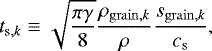$$t_{\text{s},k}\equiv \sqrt{\frac{\pi \gamma }{8}}\frac{{\rho }_{\text{grain},k}}{\rho }\frac{s_{\text{grain},k}}{c_{\text{s}}},$$(4)

where ρ is the total density of the gas and dust mixture, c_s is the sound speed of the gas, and γ its adiabatic index.

If the differential velocity Δv_k ≡v_k −v_g between the gas and the dust is supersonic, a correction in the drag regime must be applied. In this case the stopping time is given by (Kwok 1975) 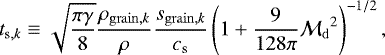$$t_{\text{s},k}\equiv \sqrt{\frac{\pi \gamma }{8}}\frac{{\rho }_{\text{grain},k}}{\rho }\frac{s_{\text{grain},k}}{c_{\text{s}}}{\left(1+\frac{9}{128\pi }{\mathcal{M}}_{\text{d}}{}^2\right)}^{-1/2},$$(5)

where ${\mathcal{M}}_{\text{d}}=\frac{|\Delta v_{\text{k}}|}{c_{\text{s}}}$ is the differential velocity Mach number. Hereafter, unless specified, we consider this correction.

In the terminal velocity approximation, the differential velocity of the phase k is $$w_{\text{k}}=\left[\frac{\rho }{\rho -{\rho }_k}{t}_{\text{s},k}-{\sum }_{l=1}^{\mathcal{N}}\frac{{\rho }_l}{\rho -{\rho }_l}{t}_{\text{s},l}\right]\frac{\nabla P_{\text{g}}}{\rho },$$(6)

and the gas and dust velocities, v_g and v_k are given by 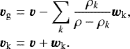$$\begin{array}{lll}{v}_{\text{g}}\hfill & =\hfill & v-{\sum }_k\frac{{\rho }_k}{\rho -{\rho }_k}{w}_{\text{k}},\hfill \\ v_{\text{k}}\hfill & =\hfill & v+w_{\text{k}}.\hfill \end{array}$$(7)

For laterpurposes, we define the dust ratio ${\varepsilon }_k\equiv \frac{{\rho }_k}{\rho },$ the total dust ratio $\varepsilon \equiv {\sum }_k^{\mathcal{N}}{\varepsilon }_k,$ and the dust-to-gas ratio ${\theta }_{\text{d}}\equiv \frac{{\sum }_k^{\mathcal{N}}{\rho }_k}{{\rho }_{\text{g}}}$. For any quantity A, we define Ā ≡ A∕A₀ where A₀ is its initial value. Here, $\overline{\varepsilon }$ and $\overline{\theta }$ are the dust-ratio and dust-to-gas-ratio enrichment, respectively. Further details about the monofluid formalism and its implementation in RAMSES can be found in Lebreuilly et al. (2019).

2.2 Dusty MHD with neutral grains

We extend the above formalism to neutral grains embedded in a weakly ionized plasma. Here, we only consider the resistive effect of ambipolar diffusion, that is, the drift between ions and neutrals other than the dust. This formalism can be straightforwardly extended to more general Ohm’s laws. In this context, the equations of dusty-magnetohydrodynamics with neutral grains (Ndusty-MHD) can be written as follows. $$\begin{array}{l}\frac{\partial \rho }{\partial t}+\nabla \cdot \left[\rho v\right]=0,\\ \frac{\partial {\rho }_k}{\partial t}+\nabla \cdot \left[{\rho }_k\left(v+w_{\text{k}}\right)\right]=0,\forall k\in \left[1,\mathcal{N}\right],\\ \frac{\partial \rho v}{\partial t}+\nabla \cdot \left[\left(P_{\text{g}}+\frac{B^2}{2}\right)\mathbb{I}+\rho (v\otimes v)-B\otimes B\right]=-\rho \nabla \varphi ,\\ \frac{\partial B}{\partial t}-\nabla \times \left[\left(v-{\sum }_k\frac{{\rho }_k}{\rho -{\rho }_k}{w}_{\text{k}}\right)\times B\right]\\ +\nabla \times \left[\frac{{\eta }_{\text{A}}{c}^2}{4\pi |B{|}^2}[(\nabla \times B)\times B]\times B\right]=0,\\ \nabla \cdot B=0,\end{array}$$(8)

where B is the magnetic field, η_A is the ambipolar resistivity, and c is the speed of light. We note that $\frac{{\eta }_{\text{A}}{c}^2}{4\pi |B{|}^2}[(\nabla \times B)\times B]$ is the differential velocity between the ions and the neutrals in the gas phase (Masson et al. 2012, 2016). We must then correct the velocity of the neutrals by accounting for the differential velocity between the gas and the barycenter. The term $-{\sum }_k\frac{{\rho }_k}{\rho -{\rho }_k}{w}_{\text{k}}$ appears in the induction equation to take this into account.

In addition to the pressure force, a magnetic force now applies on the plasma. In a previous study, Laibe & Price (2014c) provided the expression of the differential velocity for a general force budget. Using this formula we find that $$w_{\text{k}}=\left[\frac{\rho }{\rho -{\rho }_k}{t}_{\text{s},k}-{\sum }_{l=1}^{\mathcal{N}}\frac{{\rho }_l}{\rho -{\rho }_l}{t}_{\text{s},l}\right]\frac{\nabla P_{\text{g}}-(\nabla \times B)\times B}{\rho },$$(9)

and we note that this expression is very similar to what Fromang & Papaloizou (2006) found for single dust species mixtures.

To further simplify Eq. (8), we assume in this paper that the plasma velocity v is the barycenter velocity which is valid when ɛ_k||w_k||≪||w_k||≪|v|. In this case, the induction equation writes $$\begin{array}{lll}\frac{\partial B}{\partial t}-\nabla \times \left[v\times B\right]\text{ }+\nabla \times \left[\frac{{\eta }_{\text{A}}{c}^2}{4\pi |B{|}^2}[(\nabla \times B)\times B]\times B\right]\hfill & =\hfill & 0.\hfill \end{array}$$(10)

3 Method

3.1 RAMSES

For this work, we take advantage of the RAMSES code (Teyssier 2002). This finite-volume Eulerian code solves the hydrodynamics equations using a second-order Godunov method (Godunov 1959) on an adaptive-mesh-refinement grid (Berger & Oliger 1984). With a proper refinement criteria, the AMR grid is a powerful tool to study multi-scale problems such as the protostellar collapse of a dense core. The RAMSES code is very effective for problems that require the treatment of magnetohydrodynamics (Teyssier et al. 2006; Fromang et al. 2006; Masson et al. 2012; Marchand et al. 2018, 2019), radiation hydrodynamics (Commerçon et al. 2011b, 2014; Rosdahl et al. 2013; Rosdahl & Teyssier 2015; González et al. 2015; Mignon-Risse et al. 2020) or cosmic rays (Dubois & Commerçon 2016; Dubois et al. 2019).

We extended the code to the treatment of dust dynamics with multiple species in the diffusion approximation and terminal velocity regime (Lebreuilly et al. 2019). The method, based on an operator splitting technique has been extensively presented and tested. It uses a predictor-corrector MUSCL scheme (van Leer 1974) and is second-order accurate in space. The solver can be used to simultaneously and efficiently model several dust species (MULTIGRAIN).

3.2 Boss and Bodenheimer test

We perform Boss and Bodenheimer tests (Boss & Bodenheimer 1979) to follow the dynamics of the dust during the first collapse and first core formation. The parameters of the setup are the initial mass of the dense core (or prestellar core) M₀, the total dust ratio ɛ₀, the temperature of the gas T_g, and a mean molecular weight μ_g. The ratio between the thermal and the gravitational energy α is 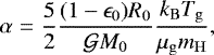$$\begin{array}{lll}\alpha \hfill & =\hfill & \frac{5}{2}\frac{(1-{\varepsilon }_0)R_0}{\mathcal{G}{M}_0}\frac{k_{\text{B}}{T}_{\text{g}}}{{\mu }_{\text{g}}{m}_{\text{H}}},\hfill \end{array}$$(11)

and sets the initial radius of the cloud R₀ and its density ρ₀. In addition, we impose an initial solid body rotation around the z-axis at the angular velocity Ω₀ by setting the ratio between the rotational and the gravitational energy β given by $$\begin{array}{lll}\beta \hfill & =\hfill & \frac{1}{3}\frac{R_0^3{\Omega }_0^2}{\mathcal{G}{M}_0}.\hfill \end{array}$$(12)

Eventually, we apply an initial azimuthal density perturbation according to $$\rho ={\rho }_0\left[1+A\cos \left(m\theta \right)\right].$$(13)

In this paper, we aim to investigate the impact of magnetic fields on the dynamics of neutral dust grains in two simulations: one with ideal MHD and one with ambipolar diffusion. For these runs, we impose a uniform magnetic field using the mass-to-flux-to-critical-mass-to-flux-ratio $$\mu =\left(\frac{M_0}{\Phi }\right)/{\left(\frac{M}{\Phi }\right)}_{\text{c}},$$(14)

the critical mass-to-flux ratio being given by ${(M/\Phi )}_{\text{c}}=\frac{0.53}{3\pi }\sqrt{5/\mathcal{G}}$ (Mouschovias & Spitzer 1976). We set an angle ϕ_mag between the magnetic fields and the rotation axis to reduce the efficiency of the magnetic braking.

3.3 Dust grain size distributions

In our MULTIGRAIN simulations, $\mathcal{N}>1$ dust bins are considered. The dust ratio of each bin is set from power-law distributions 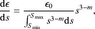$$\frac{\text{d}\varepsilon }{\text{d}s}=\frac{{\varepsilon }_0}{{\displaystyle {\int }_{S_{\text{min}}}^{S_{\text{max}}}{s}^{3-m}}\text{d}s}{s}^{3-m},$$(15)

with ɛ₀ being the total initial dust ratio, and S_min and S_max being the minimum and maximum sizes of the grains present in the medium, respectively. For the standard MRN distribution, S_min = 5 nm, S_max = 250 nm, and m = 3.5.

The method described in Hutchison et al. (2018) is used to compute the initial dust ratio and typical grain size of each bin. A logarithmic grid is used to determine the edges S_k of the bins 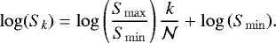$$\log (S_k)=\log \left(\frac{S_{\text{max}}}{S_{\text{min}}}\right)\frac{k}{\mathcal{N}}+\log \left(S_{\text{min}}\right)\text{}.$$(16)

The typical grain size of a bin k required to compute the stopping time is 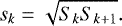$$s_k=\sqrt{S_k{S}_{k+1}}.$$(17)

We note that S_min and S_max are the edges of the distribution and must not be confused with the minimum and maximum bin size that are averaged quantities. The initial dust ratios in each bin are computed according to $${\varepsilon }_0{}_k={\varepsilon }_0\left[\frac{S_{k+1}^{4-m}-S_k^{4-m}}{S_{\text{max}}^{4-m}-S_{\text{min}}^{4-m}}\right].$$(18)

3.4 Setup

3.4.1 Cloud setup

We impose initial conditions that are typical of the first protostellar collapse (Larson 1969) with T_g =10 K, μ_g = 2.31, and a solar mass cloud. We also set γ = 5∕3 since molecular hydrogen behaves as a monoatomic gas at low temperatures (Whitworth & Clarke 1997). As explained in Sect. 2.1, a barotropic law is used to close Eq. (1) with ρ_ad = 10⁻¹³g cm⁻³ (Larson 1969). Finally, we always set m = 2 and A = 0.1 to favor fragmentation and the formation of two spiral arms.

For the dust, we always consider ten bins with grain sizes distributed according to Sect. 3.3. In all the models, S_min = 5 nm and m = 3.5, and S_max is specified individually. In all our models we set ρ_grain = 1 g cm⁻³. Finally, we impose a uniform initial total dust-to-gas ratio of θ_d,0 = 0.01 in all the models.

The two magnetic models have been computed with μ = 5 and ϕ_mag = 40°. For the nonideal MHD model the ambipolar resistivity is computed similarly to the case of reference of Marchand et al. (2016).

3.4.2 Numerical setup

We use the HLLD Riemmann solver (Miyoshi & Kusano 2005) for the barycenter part of the conservation equations with a MINMOD slope limiter (Roe 1986) for both the gas and the dust. The Truelove criterion (at least four point per Jeans length, Truelove et al. 1997) must be satisfied to avoid artificial clump formation. We therefore enforce a refinement criterion that imposes at least 15 points per local Jeans length. The grid is initialized to the level ℓ_min = 5 and allows refinement up to a maximum level ℓ_max = 16 (which gives a resolution between 32³ and 65536³ cells).

3.4.3 Analysis of the models

We considerthat the first hydrostatic core (FHSC) is fully formed when the peak density reaches 10⁻¹¹ g cm⁻³ for the first time. We denote the corresponding time t_core, and use thisdefinition to compare our models at similar evolutionary stages. We present here the different objects that are observed in our model and their definition in this work.

• The first hydrostatic core and the fragments are any object of density larger than 10^−12.5 g cm⁻³, as in Lebreuilly et al. (2019). The FHSC or ${\mathcal{F}}_0$ corresponds to the central fragment. ${\mathcal{F}}_1$ and ${\mathcal{F}}_2$ are the secondary fragments or the secondary FHSC.

• The disk $\mathcal{D}$ is the region that satisfies Joos et al. (2012) criterion. For the analysis, we place ourselves in cylindrical coordinates (r, ϕ, z). A region is identified as a disk if it is Keplerian (v_ϕ > f_threv_r), in hydrostatic equilibrium (v_ϕ > f_threv_z), rotationally supported ($\frac{1}{2}\rho v_{\varphi }^2>f_{\text{thre}}{P}_{\text{g}}$), and dense ρ > 3.9 × 10⁻¹⁵ g cm⁻³. As in Joos et al. (2012), we choose f_thre = 2.

• The pseudo-disk $\mathcal{P}$ (Galli & Shu 1993), for magnetic runs, is defined as the regions with r < 5000 AU and densities above 3.9 × 10⁻¹⁷ g cm⁻³ that are not in the disk or fragments. The criterion is similar to that used in Hincelin et al. (2016). Here, 5000 AU is an arbitrary distance that is sufficiently larger than the central objects while being smaller than the initial cloud.

• Jets/outflows $\mathcal{O}$ correspond to any region with r < 5000 AU with $v\cdot \frac{r}{\left|r\right|}>0.2 \text{km}{\text{s}}^{-1}$. This criterion is also similar to the one used in Hincelin et al. (2016).

• The envelope $\mathcal{E}$ encompasses the regions with r < 5000 AU that exclude the fragments, the disk, the pseudo-disk, the jets and the outflows.

We consider two different weights for averaging a quantity A over a volume $\mathcal{V}$ in the computational box. Volume averaging is computed according to 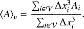$$<A{>}_v=\frac{{\sum }_{i\in \mathcal{V}}\Delta x_i^3{A}_i}{{\sum }_{i\in \mathcal{V}}\Delta x_i^3}.$$(19)

Mass averaging is computed according to 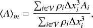$$<A{>}_m=\frac{{\sum }_{i\in \mathcal{V}}{\rho }_i\Delta x_i^3{A}_i}{{\sum }_{i\in \mathcal{V}}{\rho }_i\Delta x_i^3},$$(20)

where ρ_i and Δx_i are the total density and length of individual cells i in the averaged volume. Volume averages emphasize regions of large spatial extension, such as the envelope, while mass averages emphasize regions of high density, such as the core+disk and the denser regions of the envelope.

3.5 Regularization of the differential velocity and dust density

The terminal velocity approximation is unrealistic in low-density regions or in shocked regions where the pressure is discontinuous (Lovascio & Paardekooper 2019). We cap the differential velocities to w_cap in our models to avoid prohibitively small time-steps and unrealistically large variations in the dust ratio in strong shock fronts. We impose w_cap = 1 km s⁻¹. To verify that this does not impact the results, we ran extra models with w_cap = 0.1 km s⁻¹, w_cap = 0.5 km s⁻¹, and w_cap = 2 km s⁻¹. A comparison between these models and our fiducial is given in Appendix A.

In our models, the drift velocity can in some regions be supersonic. To account for the correction presented in Eq. (5), we use the drift velocity estimated at the previous time-step to estimate the differential velocity mach number.

Finally, we set the drift velocity to zero at densities lower than those of the initial cloud, i.e., the background. This is a way to ensure that the regions where the terminal velocity is not valid do not significantly affect the calculation.

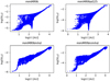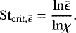
Fig. 1 Logarithm of the maximum (10th bin) Stokesnumber as a function of the spherical radius for the four models with the largest Stokes numbers at tcore + 2 kyr. Top-left: MMMRN, top-right: MMMRNA0.25, bottom-left: MMMRNMHD, bottom-righ: MMMRNNIMHD.

3.6 Validity of the model

The diffusion approximation is valid as long as the ratio between the stopping time and the dynamical timescale of the gas is small compared to unity (Laibe & Price 2014c). This ratio is called the Stokes number St.

During the first collapse, the dynamical timescale is the free-fall time t_ff. We have shown in Lebreuilly et al. (2019) that for an initial dust-to-gas ratio of 0.01 and a temperature of 10 K, the initial Stokes number St₀ of a spherical collapse is given by 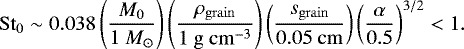$${\text{St}}_0~0.038\left(\frac{M_0}{1M_{\odot }}\right)\left(\frac{{\rho }_{\text{grain}}}{1\text{g}{\text{cm}}^{-3}}\right)\left(\frac{s_{\text{grain}}}{0.05\text{cm}}\right){\left(\frac{\alpha }{0.5}\right)}^{3/2}<1.$$(21)

The dynamics of grains smaller than 0.05 cm can be simulated using the diffusion approximation. We note that the Stokes number varies as $\propto \frac{1}{\sqrt{\rho }}$ (since $t_{\text{ff}}\propto \frac{1}{\sqrt{\rho }}$ and $t_{\text{s}}\propto \frac{1}{\rho }$) and hence can increase with a decreasing density. Figure 1 shows the values of the maximum Stokes number as a function of the radius for the four models with the least coupled dust (see Sect. 4 for a description of the models). The maximum value for St is smaller than ~ 0.15 in the external regions of the collapse for all our models and this value is typically smaller than 0.05 inside the collapsing regions of the models. Rotation provides an additional support to the collapse, which causes an increase of the free-fall timescale. Hence, as the initial angular velocity increases, the initial Stokes number decreases and the diffusion approximation is even more accurate. Similarly, magnetic fields increase the duration of the collapse which broadens the validity domain of the diffusion approximation. Finally, the Stokes number also decreases when α decreases, implying that the diffusion approximation remains valid for small values of α.

In the induction equation, we consider for simplicity that the plasma is moving at the barycenter velocity. This approximation is valid when ɛ ≪ 1, that is, when the back-reaction from the dust onto the gas is negligible. We note that we investigate the impact of the back-reaction in Appendix B.

4 Models

The models presented in this section are referenced in Table 1. All of them were evolved up to at least 2 kyr after the formation of the first core. Our fiducial case MMMRN was run over a longer time.

4.1 Fiducial simulation

In this section, we present our fiducial case MMMRN where α = 0.5 and β =0.03. The grain size distribution is extended up to S_max = 1 mm. The value of S_max leads to an average size of the last and largest bin s₁₀ ~ 160 μm. The total initial dust-to-gas ratio is θ_d,0 = 1%.

Figure 2 shows edge-on (four top figures) and mid-plane (four bottom figures) density cuts of the gas (left) and of the dust fluid with the largest grain size (160 μm, right) at 1 and 2 kyr after the formation of the first Larson core (t_core = 72.84 kyr for this model), respectively. The density distributions obtained for the gas and the dust are clearly different. This discrepancy originates from an imperfect coupling between the two phases which causes a drift of the dust toward the inner regions of the collapse. This generaltrend can be explained by a simple force budget on the gas and the dust. Although the gas is partially supported by pressure, dust grains are only subjected to gravity and gas drag. As such, the dust fluid collapses essentially faster than the gas. It therefore enriches the first core and the disk at the cost of a depletion of solids in the envelope. Figure 2 shows that this strong enrichment in the mid-plane and depletion in the envelope have already occurred at t_core + 1 kyr, and continue for more than 1 kyr. In the mid-plane, the envelope is enriched in large dust grains close to the central object and depleted further away. In the vertical direction, it is mostly depleted in large grains. In short, after the first core formation these grains are concentrated in a very thin layer of 10−100 AU above/under the mid-plane. At this stage, the envelope is mostly a reservoir of low dust densities for the large grains. Hence accretion of dust arising from the envelope does not significantly enrich the fragments or the disk with large grains and the dust-to-gas ratio in the disk even decreases. We note that the disk is still very enriched by the end of the calculation. Most of the enrichment of the dust-to-gas ratio in the central objects indeed takes place during the initial phases of the collapse, when the densities are low everywhere and the coupling between the gas and the dust is the weakest.

Figure 3 shows probability density functions (PDFs) of the dust ratio enrichment, denoted $\log (\overline{\varepsilon })$. Here we compare the distributions of the two most coupled and the three least coupled dust species (colored dashed lines) at t_core + 2 kyr. We also indicate the PDFs integrated over the grain size distribution (black line). These PDFs are displayed in three different regions, namely the core and the fragments (left), the disk (middle), and the envelope (right). Figure 3 shows that the dust enrichment in the inner regions is size dependent. Smaller grains experience larger drag that reduces their differential velocity with respect to the gas.

Here, grains with sizes smaller than a few microns remain very well coupled with the gas in all the considered regions, whereas for larger grains the PDF of the dust ratio is broad. For 160 μm grains, the dust ratio increases by one order of magnitude in some regions of the disk and up to two orders of magnitude in the envelope. On average, the dust ratio is 0.018 in the core, 0.0175 in the disk, and ~ 0.0086 in the envelope. In addition, the dust has experienced a strong and local dynamical sorting. We indeed measure a typical standard deviation for the dust-ratio enrichment $\overline{\varepsilon }$ of 0.072 in the core, 0.14 in the disk, and 0.23 in the envelope. The standard deviation is the largest in the envelope, a region which is depleted in dust in the outer regions and enriched close to the disk and fragments. The disk experiences larger variations of dust-to-gas ratio compared to the core. Indeed, the latter is in adiabatic contraction. This induces high temperatures, which in return causes a strong decrease of the Stokes number. Hence, dust is essentially frozen with the gas in the core and v_d ≈v_g. Figure 4 shows the dust ratio for the total dust distribution (left) and for the tenth species (right) in the mid-plane of the collapse, at 1 kyr (top), 2 kyr (middle), and 4 kyr (bottom) after the formation of the first Larson core, respectively. The maps on the left and on the right are very similar as most of the evolution of the dust ratio is due to the dynamics of the least coupled species, which represents a large fraction of the dust mass (see also the PDF). The structures in the dust ratio observed in Fig. 4 can be interpreted by looking at the thermal pressure distribution shown in Fig. 5. Dust grains tend to drift toward local pressure maxima (see Fig. 4, top panel) where the differential velocity is zeroed (see Eq. (6)). The greatest variations of the total dust ratio are due to the largest grains, since they represent most of the dust mass and have the largest drift velocities. Hence, a significant fraction of the dust mass in the inner regions is composed of large grains. Finally, we note that 4 kyr after the first core formation, the average value for the total dust-to-gas ratio remains roughly unchanged but generally increases (of about 1%) in the core and fragments after their formation. For the disk, we note a decrease in the dust ratio of ~ 30% for the largest grains (~22% in total) in the disk following the first core formation. In addition, the total dust-to-gas ratio continues to diminish in the envelope at this time as settling goes on, with a final average value of ~ 0.0083.

Figure 6 shows the evolution of the dust-to-gas ratio enrichment averaged in volume for different density thresholds in the regions where R < 5000 AU. The dust depletion at large scales in the envelope at low densities is a relatively slow process, which occurs during the entire collapse. Once regions with larger densities are formed, they usually experience a relatively quick enrichment from the dust content of the low-density regions, and then a quick depletion in favor of even denser regions. Figure 6 shows that fragmentation occurs in a dust-rich environment. A strong enrichment of the volume where ρ > 10⁻¹³ g cm⁻³, delimited by the brown line, indeed happens exactly when fragments form. This explains why these fragments tend to be more dust-rich than the first hydrostatic core. Interestingly, the dust-to-gas ratio does not vary significantly in the volume where ρ > 10⁻¹¹ g cm⁻³ which is in adiabatic contraction. Again, the temperatures in this region are high and therefore the Stokes numbers are very low, which significantly slows down the differential dynamics of the gas and the dust. We note that this volume is already dust enriched by almost a factor of two by the time of its formation.

4.2 Parameter exploration

4.2.1 Maximum grain size

As seen in Sect. 4.1 for the MMMRN model, the differential dynamics between gas and dust during the protostellar collapse depend critically on grain size. Therefore, we perform two simulations 100MICMRN and MRN with the same set of parameters as in MMMRN, but with a different maximum grain size. We choose S_max = 100 μm for the 100MICMRN model (which yields s₁₀ ~ 22.6 μm) and S_max = 250 nm for the MRN model (which yields s₁₀ ~ 139 nm).

Let us first consider MRN, which is the model that has the smallest S_max. Figure 7 shows the density of the gas (left) of the least coupled dust species (right) at t_core + 2 kyr. Because the coupling between gas and dust is almost perfect, the two maps are indistinguishable by eye. This is expected because the maximum grain size is ≈ 10⁻⁵ cm which corresponds to an initial Stokes number St_0,10 ~ 1.06 × 10⁻⁵ ≪ 1 (see Sect. 6 for a theoretical justification). As a result, dust is an excellent tracer of gas in this model. This is illustrated by Fig. 8, which shows the probability density function of the dust ratio enrichment $\log (\overline{\varepsilon })$ in the core and fragments, the disk, and the envelope at t_core + 2 kyr. Contrary to the MMMRN model, these PDFs are strongly peaked. The average dust-to-gas ratio integrated over the total dust distribution is ≈ 1% in the core andthe fragments, the disk, and the envelope. The standard deviation for the dust ratio enrichment ranges between 2 × 10⁻⁴% (in the core) and 1.4 × 10⁻²% (in the envelope). For this model, the variations of the dust ratio are very small. Therefore, in absence of coagulation, one may expect a standard MRN distribution to remain extremely well preserved during the protostellar collapse at all scales.

To investigate an intermediate scenario, we now focus on the 100MICMRN model. We do not show the density maps in this case due to their strong resemblance with the MRN case. The PDFs of the dust ratio enrichment $\log (\overline{\varepsilon })$ in the core and fragments, the disk, and the envelope at t_core + 2 kyr are shown in Fig. 9. In this case, the variations of dust ratio are more significant than in MRN. However, compared to the MMMRN case, these variations still remain quite small. The average dust-to-gas ratio is 0.0106 in the core and the disk and 0.0099 in the envelope. The typical standard deviation for the dust-ratio enrichment are 7 × 10⁻³ in the core, 2.2 × 10⁻² in the disk, and 7.8 × 10⁻² in the envelope. This confirms that the larger the grains are, the more significant the decoupling with the gas. We note that, for 100MICMRN, it is reasonable to infer the gas density from the dust.

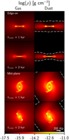Fig. 2 MMMRN test at tcore + 1 kyr and tcore + 2 kyr (tcore =72.84 kyr). Edge-on and mid-plane cuts of the gas and the dust densities for the least coupled species are provided (left and rights respectively). Values of the gas density are indicated by the colorbar at the bottom. Dust densities have been multiplied by a factor 100 to be represented on the same scale. Hence, colors of the gas and the dust maps match when the dust-to-gas ratio equals its initial value 0.01. Dust densityvariations in regions where ɛ0ρd < min(ρg) have voluntarily not been displayed to highlight the enriched regions. These depleted regions are delimited by the dashed gray lines. This choice of colors applies for all density maps in this study. Gas and dust are clearly not perfectly coupled.

4.2.2 Thermal-to-gravitational energy ratio

The free-falltimescale depends on the ratio between the thermal and the gravitational energy. We therefore present in this section MMMRNA0.25, a model similar to the reference case but with α = 0.25. This parameter is expected to strongly affect the dust dynamics. A lower value of α produces faster protostellar collapses prior to the first core formation due to the smaller thermal support. It therefore develops high-density regions more quickly, where dust strongly couples. In addition, a cloud with a smaller α has a smaller initial Stokes number, which means that the dust is also initially better coupled with the gas. The post-core evolution of MMMRNA0.25 is different from that inMMMRN in virtue of a smaller initial disk radius. Smaller disks with a smaller initial value of α are expected as shown by Hennebelle et al. (2016; their Eq. (14)).

Figure 10 shows the densities of the gas (left) and the least coupled dust species (right) at t_core + 2 kyr for MMMRNA0.25. Apart from the outer regions that are quite depleted in dust content, we do not see any significant difference between gas and dust. Indeed, the core forms quickly, leaving no time for the differential motion between gas and dust to develop. For a comparison with the fiducial case, we show in Fig. 11 the PDF of the dust ratio enrichment $\log (\overline{\varepsilon })$ in the core and the fragments, the disk, and the envelope at t_core + 2 kyr. The PDFs are much more peaked in MMMRNA0.25 than in MMMRN. The values of the standard deviation of the dust-ratio enrichment are 2 × 10⁻² in the FHSC and fragments, 3 × 10⁻² in the disk, and 0.1 in the envelope. This was actually expected as the initial Stokes number scales as α^2∕3 and is thus ≈ 0.6 times smaller in MMMRNA0.25 than in MMMRN.

4.2.3 Magnetic fields

We now consider the dynamics of neutral grains in collapsing magnetized clouds. The two models are performed with the same parameters as MMMRN but with an initial magnetic field given by μ = 5 and a tilt of 40°. For MMMRNMHD we use an ideal MHD solver and for MMMRNNIMHD we consider ambipolar diffusion.

Figures 12 and 13 show the densities for the gas (left) and the least coupled dust species (right) at t_core + 2 kyr for the two models MMMRNMHD and MMMRNNIMHD, respectively.For both models, the dust is significantly decoupled from the gas and the settling in the core/disk/pseudo-disk is very efficient. As in MMMRN, dense regions (disk, core, pseudo-disk, and high-density regions of the outflow) are prone to be enriched in solid particles while low-density regions are depleted(envelope and low-density regions of the outflow). We note that the decoupling is slightly more efficient in these models than in MMMRN. This is mostly due to the 10 kyr difference in free-fall timescale. Although additional decoupling terms due to the magnetic field appear in the dust differential velocity (∝J ×B see Eq. (9)) those are negligible compared to the hydrodynamical terms (∝ ∇P_g) in the decoupling of gas and dust in our magnetised collapse models.

Figures 14 and 15 show the PDFs of the dust ratio enrichment for the different objects at t_core + 2 kyr for the MMMRNMHD and MMMRNNIMHD runs, respectively. Although the shapes of the distributions are different from our fiducial case, we essentially reach the same conclusion, that is, a peaked distribution with a significantly large average, indicating a strong initial enrichment in the [core+disk] system and a broad distribution in the envelope. We note that the average dust-to-gas ratio in the disk and the core is higher in these two models than in the fiducial case. We indeed measure an average dust-to-gas ratio of ~ 0.022−0.023 in the disk and the first hydrostatic core for these models. In these magnetic runs, the pinching of the magnetic field lines during the collapse produces a pseudo-disk, which is a dense but not rotationally supported region. We note that these pseudo-disks have a very broad PDF and show enriched and depleted regions in both the ideal and nonideal cases. Similar behavior is observed in the magnetically driven outflow for the ideal case, which is dust-rich in dense regions and depleted at low densities. In the MMMRNNIMHD, the outflow is less evolved and is mostly dust-depleted, similarly to the envelope.

In summary, neutral dust dynamics in the presence of magnetic fields seem to follow the same general trend as in the hydrodynamical case. Dust collapses faster than the gas and is enriched in the inner regions of the collapse a few thousand years after the first core formation. This enrichment is mainly located in the pseudo-disk (only observed in the magnetized models), the disk, the first hydrostatic core, and the high-density regions of the outflow.

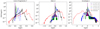Fig. 3 MMMRN test at tcore + 2 kyr: probability density function (PDF) of the dust ratio enrichment $\log (\overline{\varepsilon })$ for the two most coupled and three least coupled dust species (colored dashed lines) and for all the dust (black line) in the core+fragments (left), the disk (middle), and the envelope (right). Dust is not a good tracer for the gas here and the dust distribution is not uniform in the considered objects.

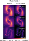Fig. 4 MMMRN test ~ 1 kyr (top), ~2 kyr (middle), and ~4 kyr (bottom) after the first core formation (tcore = 72.84 kyr). Mid-plane view of the total dust ratio (left) and the dust ratio of the least coupled species (right). The colorbar is the same for both figures. The dotted white lines represent the regions where the total (left) or 160 μm grain (right) dust-to-gas ratio is at its initial value, which can also be regarded as a dust enrichment line.

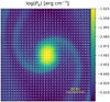Fig. 5 MMMRN test at tcore + 1 kyr (tcore =72.84 kyr). Mid-plane view of the gas pressure (up-close). The white arrows represent the direction of the differential velocity w10.

5 Features of dusty collapses

We summarize here the properties of the dusty collapse in its different regions. Figure 16 shows the dust-to-gas ratio enrichment averaged in mass as a function of the grain size for all the models and all the objects defined in Sect. 3.4.3. We refer to the dashed horizontal line as the enrichment line; if an object lies above this line, it is enriched in dust during the collapse; if it lies underneath, it is dust depleted. This information is collected in Table D.2.

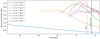Fig. 6 MMMRN test. Volume averaged total dust-to-gas ratio enrichment as a function of time for different density thresholds.The FHSC formation can be identified by the dotted vertical blue line while fragmentation occurs during a time delimited by the green area. We observe a slow decrease of the dust-to-gas ratio at low density which gives rise to an enrichment of high-density regions. Cores and fragments at ρ > 10−11 g cm−3 are formed in a dust-rich environment. The dust-to-gas ratio is almost constant for ρ > 10−11 g cm−3 because the increase of temperature due to the adiabatic contraction strengthens the coupling between the gas and the dust.

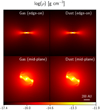Fig. 7 MRN test at tcore + 2 kyr (tcore =73.6 kyr). Edge-on (top) and mid-plane (bottom) cuts of the gas density (left) and dust density of the least coupled species (right). The two maps are almost indistinguishable due to the very strong coupling between gas and all dust species.

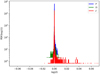Fig. 8 MRN test at tcore + 2 kyr. Probability density function (PDF) of the total dust ratio enrichment $\log (\overline{\varepsilon })$ in the core and the fragments, the disk, and the envelope. Dust is a very good tracer of mass here and the dust distribution is almost uniform in the objects considered.

5.1 Core and fragments

Here we detail the dust and gas properties in the first hydrostatic core and the fragments. In every model, we observe a value of $<{\Theta }_{d,k\le 6}{>}_m$ that remains unchanged for all the cores and fragments. Indeed, small grains have short stopping times and remain verywell coupled to the gas all along the collapse. Simulations with the largest maximum grain size (S_max = 0.1 cm) have the largest dust enrichment. On the contrary, for the MRN model, the dust-to-gas ratio preserves its initial value in all the fragments. Moreover, the dust distribution itself remains extremely well preserved. In the MMMRNA0.25 case, the enrichment of the largest dust grains is much less efficient than in MMMRN. This is explained by a shorter free-fall timescale and higher initial densities, which implies smaller initial Stokes numbers. In MMMRN, MMMRNA0.25, and 100MICMRN, the fragments have greater enrichment in larger grains (k > 6, see Table D.1 for the corresponding grain sizes). For example, in the MMMRN case, the dust-to-gas ratio of the 160 μm grains is enriched by a factor of ≈2.6 in the central object, and ≈3 in the fragments. We note that the dust-to-gas ratio enrichment of the first hydrostatic core is stronger in simulations that include magnetic fields than in MMMRN. As explained above, magnetic fields bring an additional decoupling in the case of neutral grains which explains in part why the dust enrichment is even stronger in MMMRNMHD and MMMRNNIMHD than in MMMRN. More importantly, the collapse is longer for these models due to the magnetic support. This leaves more time for dust grains to enrich the central regions. For the fragmenting cases, we note a preferred concentration of dust in the fragments, which can be explained by two mechanisms. First, fragments form after the central object and thus remain for longer in the isothermal phase where dust is less coupled because the temperature is lower. Second, the dust-rich spiral arms developing through the envelope (see Fig. 4) are mainly accreted by the fragments (see Fig. 6). This provides an additional channel to enrich the fragments in solids.

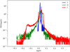Fig. 9 100MICMRN test at tcore + 2 kyr. Probability density function of the total dust ratio enrichment $\log (\overline{\varepsilon })$ in the core and the fragments, the disk, and the envelope. Dust is a relatively good tracer of gas although significant variations of the dust-to-gas ratio are observed.

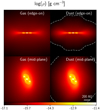Fig. 10 MMMRNA0.25 test at tcore + 2 kyr (tcore =23 kyr). Edge-on (top) and mid-plane (bottom) cuts of the gas density (left) and dust density of the least coupled species (right). Dust has less time to significantly decouple from the gas than in the MMMRN case. A strong dust depletion is observed in the envelope.

Fig. 11 MMMRNA0.25 test at tcore + 2 kyr. Probability density function of the total dust ratio enrichment $\log (\overline{\varepsilon })$ in the core+fragments, the disk, and the envelope. Dust is a relatively good tracer for gas in the dense object although a notable depletion is observed in the envelope.

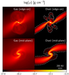Fig. 12 MMMRNMHD at tcore + 2 kyr (tcore =81.1 kyr). Edge-on (top) and mid-plane (bottom) cuts of the gas density (left) and dust density of the least coupled species (right). Dust is significantly decoupled from the gas and concentrates in the high-density regions such as the core, the disk, the pseudo-disk,and the inner regions of the outflow.

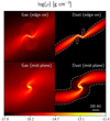Fig. 13 MMMRNNIMHD at tcore + 2 kyr (tcore =81.1 kyr). Edge-on (top) and mid-plane (bottom) cuts of the gas density (left) and dust density of the least coupled species (right). As in the ideal case, dust is significantly decoupled from the gas and concentrates in the high-density regions such as the core, the disk, the pseudo-disk, and the inner regions of the outflow.

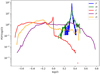Fig. 14 MMMRNMHD test at tcore + 2 kyr. Probability density function of the dust ratio enrichment $\log (\overline{\varepsilon })$ in the core (blue), the disk (green), the pseudo-disk (purple), the outflow (orange) and the envelope (red). Dust is not a good tracer of gas here and the dust distribution is not uniform in the considered objects.

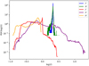Fig. 15 MMMRNNIMHD test at tcore + 2 kyr. Probability density function of the dust ratio enrichment $\log (\overline{\varepsilon })$ in the core (blue), the disk (green), the pseudo-disk (purple), the outflow (orange) and the envelope (red). Dust is not a good tracer of gas here and the dust distribution is not uniform in the considered objects.

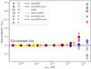Fig. 16 All the models at tcore + 2 kyr. The dust-to-gas ratio enrichment averaged in mass is shown as a function of grain size for all the objects. Grains with sizes smaller than 10−4 cm are almost always perfectly coupled with the gas. For larger grain sizes, the enrichment is model dependent. Grains with typical sizes larger than 10−3 cm decouple from the gas. Dense objects such as the fragments $\mathcal{F}$ or the disk $\mathcal{D}$ and pseudo-disk $\mathcal{P}$ are enriched in dust. Low-density objects such as the envelope $\mathcal{E}$ or the outflows $\mathcal{O}$ are depletedin dust. Magnetized models exhibit the strongest decoupling between the gas and the dust.

5.2 Disks

We review the disk properties of all the models at t_core + 2 kyr. In general, the values are similar to what is measured in the cores. This is mostly caused by the fact that the dust enrichment happens prior to core formation at low densities (see Fig. 6). We measure a total dust-to-gas ratio enrichment of ~ 1.75 in MMMRN, ~ 1 in MRN, ~ 1.1 in 100MICMRN, ~ 1.1 in MMMRNA0.25, ~ 2.3 in MMMRNMHD, and ~ 2.1 in MMMRNNIMHD. We emphasize once again that the decoupling between the gas and the dust depends strongly on the initial properties of the cloud. We note that in MMMRN the dust ratio is highly nonuniform in the disk (see Figs. 3 and 4 for the MMMRN case) or even constant (see Fig. 6). As explained in Sect. 4.1, there is a decrease of ~ 22% of dust-to-gas ratio in MMMRN between t_core and t_core + 4 kyr. This is most likely due tothe fact that the disk is accreting dust-depleted material from the envelope. In addition, since dust drifts toward pressure bumps – or regions where J ×B ~∇P_g for magnetic runs – dust cannot always be used as a direct proxy to trace the gas density. Although the substructures seen in the dust originate from those in the gas, as shown in Fig 5, they may have very distinct morphologies. This is similar to what is found for T Tauri disks, where gaps could be opened in the dust only (Dipierro & Laibe 2017). Once again, simulations with magnetic fields show a more significant dust enrichment because of the longer timescale of the collapse. We note that the disk masses are however much smaller in the two models where magnetic braking occurs. Indeed, a longer integration time is required for the disk to grow significantly (Hennebelle et al. 2020).

5.3 Pseudo-disks

In this section, we describe the principal features of the dusty pseudo-disks that are observed in the two magnetic runs MMMRNMHD and MMMRNNIMHD. These pseudo-disks are strongly enriched with a total dust-to-gas ratio enrichment of approximately two for both cases (see values in Table D.2). Interestingly, the pseudo-disk is generally more enriched in smaller grains (up to 47 μm grains) thanthe other objects. This is due to two effects. First, the pseudo-disk is less dense than the central regions of the collapse, namely the disk and the core; this explains why smaller grains drift more easily towards it. Second, the strong pressure gradient orthogonal to the pseudo-disk generates a drift from the envelope towards it, even for small grains. Once these grains have reached the pseudo-disk, they couple strongly to the gas while larger grains are able to drift to even deeper regions such as the disk andthe core.

5.4 Outflows

We now describe the major features of the dusty outflows that can be observed in the two magnetic runs MMMRNMHD and MMMRNNIMHD. For MMMRNMHD, Fig. 17 shows the relative variations of the dust ratio at three different times, for the 47 μm (left) and 160 μm (right) grains (ninth and tenth bins), respectively. The magenta arrows represent the differential velocity with the barycenter. These two dust species have a completely different evolution. Indeed, the outflow does not carry a significant quantity of 160 μm grains at t_core + 2 kyr because they are already strongly depleted in low-density regions. Subsequently, the outflow is strongly depleted in these species with $<{\overline{\Theta }}_{\text{d},10}{>}_m~0.22$ for MMMRNMHD and $<{\overline{\Theta }}_{\text{d},10}{>}_m~0.44$ for MMMRNNIMHD. On the contrary, 47 μm grains are significantly enriched by a factor 1.04–1.28 at that time. Initially, the outflow is not powerful enough to eject matter from the inner regions and rather collects the grains from the envelope. This explains why the enrichment measured in the outflow is similar to those measured in the envelope. Interestingly, at t_core + 2 kyr, we see that the outflow is well established and starts to carry the inner regions that are denser and more enriched in 160 μm grains. This indicates that outflows provide a channel to re-enrich the envelope in large grains.

5.5 Envelope

In general, the envelope is dust depleted owing to mass conservation since the inner parts are enriched. For all the models, the small dust grains (with k ≤ 6) do not experience significant dust-to-gas ratio variations. Larger grains can however show significant dust-to-gas ratio variations. We measure a value of $<{\Theta }_{d,10}{>}_m$ as low as 0.38 for MMMRNNIMHD and MMMRNMHD, and 0.73 for MMMRN. These values are averaged over the whole envelope, but contrary to the core and fragments, the envelope is very contrasted in terms of density. Among all objects (pseudo-disk excluded), the envelope experiences the largest dust-to-gas ratio variations (see e.g., Figs. 3 and 15). This is expected since the density in the envelope is lower than in the other objects. Typically, the large-grain depletion in the envelope increases with decreasing density and there is a larger dust content in its inner regions (see Fig. 17 for both behavior).

We have shown that dust is not necessarily a good tracer of gas density, that is, we find important local variations in the dust distribution in MMMRN, MMMRNMHD, and MMMRNNIMHD. This has significant consequences for observations, since dust continuum radiation fluxes depend on densities integrated along the line of sight. It is therefore interesting to estimate the error that arises when the total column density is estimated from the mass of a single dust bin k. We compute this error Err_k from the total column density and the dust column density Σ_d,k according to 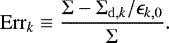$${\text{Err}}_k\equiv \frac{\Sigma -{\Sigma }_{\text{d},k}/{\varepsilon }_{k,0}}{\Sigma }.$$(22)

The total error Err is defined inthe same way but using the total dust column density and initial dust ratio.

Figure 18 shows an edge-on view of the total column density Σ (top), the total error Err (middle), and the error estimated using the largest grains only – 160 μm in this case (bottom) for the MMMRNNIMHD model 2 kyr after the formation of the first core. The error is large when considering either all the grains (middle) or only the largest ones (bottom). We note that the total column density inferred from the total dust mass would be underestimated in the upper layers and overestimated in the inner regions because dust drifts toward the center of the collapse. The effect is maximal for the largest grains, where the error can reach values as high as ~ 250% in the inner envelope.

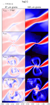Fig. 17 mmMRNmhd. Edge-on view of the relative variations of the dust ratio at four different times for the 47 μm (left) 160 μm grains (right). The magenta arrows represent the differential velocity with the barycenter. Regions that are dust depleted by more than two orders of magnitude are not displayed (black background).

6 Estimate of the dust enrichment

Here, we provide a semi-analytic estimate of the dust enrichment occurring during the protostellar collapse. We use it to infer the typical minimal Stokes number above which a given dust enrichment can be reached.

6.1 Enrichment equation

In the terminal velocity approximation, and making the assumption that the collapse is isothermal and purely hydrodynamical, the evolution of the dust ratio for a species k is given by $$\frac{\text{d}{\varepsilon }_k}{\text{d}t}=-\frac{1}{\rho }\nabla \cdot \left[{\varepsilon }_k\left(\frac{t_{\text{s},k}}{1-{\varepsilon }_k}-{\sum }_{i=1}^{\mathcal{N}}{\varepsilon }_i\frac{t_{\text{s},i}}{1-{\varepsilon }_i}\right)c_{\text{s}}^2\nabla \rho \left(1-{\sum }_{j=1}^{\mathcal{N}}{\varepsilon }_j\right)\right].$$(23)

To provide analytical estimates of dust-ratio enrichment during the collapse, we now neglect the cumulative back-reaction of dust onto the gas. When the cumulative back-reaction is negligible, the evolution of $\overline{\varepsilon }=\frac{\varepsilon }{{\varepsilon }_0}$ and ɛ are constrained by the same equation, that is, $\overline{\varepsilon }$ does not depend on ɛ₀. The dust ratio enrichment is described by the equation $$\frac{\text{d}\overline{{\varepsilon }_k}}{\text{d}t}=-\frac{1}{\rho }\nabla \cdot \left[\overline{{\varepsilon }_k}{t}_{\text{s}}{c}_{\text{s}}^2\nabla \rho \right],$$(24)

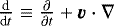where $\frac{\text{d}}{\text{d}t}\equiv \frac{\partial }{\partial t}+v\cdot \nabla$. We now use the dimensionless variables $$\tau =\frac{t}{{\tau }_{\text{ff},0}} \text{and} x=\frac{r}{{\lambda }_{\text{J},0}},$$

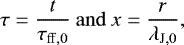
where ${\tau }_{\text{ff},0}=\sqrt{\frac{1}{\mathcal{G}{\rho }_0}}$ and λ_J,0 = c_sτ_ff,0. Equation (24) becomes $$\frac{\text{d}\overline{{\varepsilon }_k}}{\text{d}\tau }=-{\text{St}}_{k,0}\frac{1}{\overline{\rho }}{\nabla }_x\cdot \left[\overline{{\varepsilon }_k}{\overline{\rho }}^{-1}{\nabla }_x\overline{\rho }\right],$$(25)

where $\overline{\rho }=\frac{\rho }{{\rho }_0}$. The term ${\overline{\rho }}^{-1}$ appears in the divergence owing to $t_{\text{s},k}\propto \frac{1}{\rho }$.

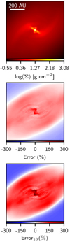Fig. 18 MMMRNMHD at tcore + 2 kyr. Edge-on view of the total column density log(Σ) (top), the total error Err (middle) and the error when using the largest grains only – 160 μm in this case (bottom).

6.2 Semi-analytical model

Neglecting local variations of $\overline{\varepsilon }$ in comparison with local density variations yields $$\frac{\text{d}\overline{{\varepsilon }_k}}{\text{d}\tau }\simeq -{\text{St}}_{k,0}\overline{{\varepsilon }_k}\frac{1}{\overline{\rho }}{\nabla }_x\cdot \left[{\overline{\rho }}^{-1}{\nabla }_x\overline{\rho }\right].$$(26)

We then obtain $$\overline{\varepsilon }\left(x,\tau \right)={\chi }^{{\text{St}}_{k,0}},$$(27)

where $\chi \equiv e^{-{\displaystyle {\int }_0^{\tau }{\nabla }_x}({\overline{\rho }}^{-1}{\nabla }_x\overline{\rho })/\overline{\rho }\text{d}\tau }$ is independent of the dust properties. Hence, at a given time and position, the dust enrichment varies essentially exponentially with the initial Stokes number. A proper mathematical estimate of the integral quantity is beyond the scope of this study.

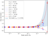Fig. 19 Semi-analytic and measured enrichment in our hydrodynamical models (MRN excluded) against the initial Stokes number. The lines represent the semi-analytical development using a best fit of χ for the FHSC (dotted), disk (solid), and envelope (dashed), respectively. The extreme values of the enrichment given by our toy model are delimited by the blue areas. The color coding and choice of markers is the same as in Fig. 16.

6.3 Estimate in the core

We can roughly approximate χ in the core and after a free-fall time $t_{\text{ff},0}=\sqrt{\frac{3\pi }{32}}{\tau }_{\text{ff},0}$. An order of magnitude estimate provides $$\left|\text{ln}\left(\chi \right)\right|\approx \sqrt{\frac{3\pi }{32}}\frac{c_{\text{s}}^2}{\mathcal{G}{\rho }_{\text{ad}}{r}_{\text{var}}^2},$$(28)

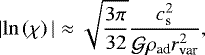
where r_var is the typical length at which variations of density become significant. Above ρ_ad, the temperature is high and the gas and dust differential dynamics is negligible. A reasonable choice for $\overline{\rho }$ is therefore $\overline{\rho }=\frac{{\rho }_{\text{ad}}}{{\rho }_0}$. In the typical condition of a protostellar collapse, one obtains $$\left|\text{ln}\left(\chi \right)\right|\approx 126{\left(\frac{r_{\text{var}}}{1 \text{AU}}\right)}^{-2}\left(\frac{T_{\text{gas}}}{10 \text{K}}\right).$$(29)

We note that taking r_var = 1 AU seems reasonable as it is about a tenth of the first-core radius in our models. For r_var ≈ 5 AU, we find that $\left|\text{ln}\left(\chi \right)\right|\approx 5$. The value of χ strongly depends on the steepness of the pressure gradients, and therefore on r_var. This model only provides a rough estimate of $\overline{\varepsilon }$ and should not replace either a numerical treatment of the dust or a proper estimate of χ during the collapse.

6.4 Comparison with the models

Figure 19 shows the dust ratio enrichment as a function of the initial Stokes number for MMMRN, MMMRNA0.25, and 100MICMRN for the first core, the disk, and the envelope. The dashed, dotted, and solid lines represent the values obtained with Eq. (27) by fitting the values of χ. Finally, the blue area represents the range of dust enrichment obtained with the two extreme values of χ estimated in the previous section. We do not show the dust enrichment for MRN as it is clearly negligible (see Fig. 16). In addition, we do not display the enrichment in the secondary fragments for the sake of readability.

Fairly good agreement between the fits and the measured dust ratio enrichment is observed in all the regions, especially in the cores. This suggests that the enrichment indeed mostly varies exponentially with the initial Stokes number. We do observe small deviations in the disk and the envelope for MMMRN. The nonlinear behavior of Eq. (23), either due to local variations of ɛ or the cumulative back-reaction of dust on the gas, is therefore not completely negligible. In Appendix B, we show that the dust-to-gas variations induced by the dust back-reaction are almost negligible and that the discrepancy with the exponential increase of the dust ratio observed is most likely caused by local variations in the dust-to-gas ratio; for example the mixing between depleted material of the envelope and dust-rich material from the disk.

Finally, we emphasize that the dust enrichment in all the cores is comprised between the lowest and highest values estimated with our toy model. As this model is relatively crude, we acknowledge that it cannot compete with an eventual model based on an accurate estimate of χ.

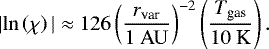
6.5 Critical Stokes number

Assuming that the value of χ is known, it can be used to determine the critical Stokes number ${\text{St}}_{\text{crit},\overline{\varepsilon }}$ above which some regions can reach a given enrichment $\overline{\varepsilon }$. Equation (27) can indeed by inverted as $${\text{St}}_{\text{crit},\overline{\varepsilon }}=\frac{\text{ln}\overline{\varepsilon }}{\text{ln}\chi }.$$(30)

Using the value of χ obtained by fitting our models (Fig. 19), we can estimate the typical Stokes numbers needed to get a dust enrichment by a factor of two in the core, and the disk is approximately St_crit,2 ~ 0.01−0.027. With our toy model, we find St_crit,2 ~ 0.006−0.13. This latter is a significantly wider range but it contains what is measured with our models. Similarly, we can estimate that to get a dust ratio depletion of 50%, the grains must typically have St_crit,1∕2 ~ 0.027−0.11. In short, it is easier to enrich the disk and the core than it is to deplete the envelope.

7 Discussion

7.1 Summary of the models

We investigated the effect of several parameters on the dust dynamics during the protostellar collapse such as the thermal-to-gravitational energy ratio α, the maximum grain size of the dust distribution, and the presence of magnetic fields. It appears that the first two parameters are critical for the development of significant differential dynamics between the gas and the dust during the early phases of the collapse.

From MMMRN, MRN, and 100MICMRN, we established that the maximum grain size is a critical parameter for the differential gas and dust dynamics. Typically, if the maximum grain size in the core is smaller than a few microns (see Fig. 16), we do not observe significant variations of the dust ratio. On the contrary, when larger grains are considered, the total dust ratio can increase by a factor of two to three, even in the very first few thousands of years of the protostellar collapse (see MMMRN, MMMRNMHD or MMMRNNIMHD). Hence, in order to understand the initial dust and gas content of protoplanetary disks, it is crucial to accurately measure thedust size distribution in early prestellar cores. This conclusion is reinforced by recent observations (Galametz et al. 2019) or synthetic observations (Valdivia et al. 2019) that seem to probe the existence of ~ 100 μm in Class 0 objects.

For small initial values of α, for example in MMMRNA0.25, the collapse is fast and large grains do not have the time to significantly enrich the core and the disk in one free-fall timescale. Besides, as MMMRNA0.25 is set with a higher initial density, dust is initially more coupled with the gas in this particular model. We point out that the efficiency of the dust enrichment relies strongly on the lifetime of low-density regions (see Fig. 6) and on the range of densities experienced during the collapse (see Sect. 6). Therefore, although 100MICMRN has a smaller maximum grain size than MMMRNA0.25, both models have a similar total dust content by the end of the simulation as the free-fall timescale in 100MICMRN is longer. The initial properties of the cloud appear to be extremely important to quantify the evolution of the dust distribution during the protostellar collapse. It would therefore be interesting to study the dust collapse of a Bonor-Ebert sphere, since its free-fall timescale is usually longer than that of the Boss and Bodenheimer test (Machida et al. 2014). We leave this proper comparison to future studies.

With MMMRNMHD and MMMRNNIMHD, we investigated the effect of a magnetic field on the dynamics of dust during the protostellar collapse. We find qualitatively similar results to those in our fiducial case. Quantitatively, the decoupling between the gas and the dust does however produce more significant variations of the dust-to-gas ratio in the magnetic case. The presence of a dense and stratified pseudo-disk strengthens the envelope and the outflow depletion. This pseudo-disk is consequently strongly enriched in solids. It is in fact almost as enriched as the disk and the first hydrostatic core. However, it is much more massive than the disk by the end of the calculation. Therefore, understanding how the pseudo-disk is accreted by the core and the disk is of particular interest and future studies should focus on its long-term evolution.

To summarize, Fig. 20 shows a schematic view of a dusty protostellar collapse a few thousand years after the formation of the first hydrostatic core. The blue areas depict the dust-depleted regions (low-density regions of the envelope and outflow) and the red areas represent the regions enriched in dust (cores, disk, high-density regions of the envelope and outflow, and pseudo-disk). The intensity of the gas and dust decoupling depends naturally on the parameters that we presented earlier in this article. We emphasize that this cartoon illustration is only a simplified picture of a dusty protostellar collapse that does not account for the variability between the models and we do not quantitatively show the local variations of the dust-to-gas ratio.

7.2 Comparison with previous works

Our results are in qualitative agreement with the previous study of Bate & Lorén-Aguilar (2017), where a decoupling between gas and dust for grains largerthan ≈100 μm was also identified. A main difference is that we do not obtain equally large dust-to-gas ratio enhancements. Indeed, in Bate & Lorén-Aguilar (2017), the dust mass is distributed in a single bin of dust with a mass of 1% of the mass of the gas. In our MULTIGRAIN simulations, only a fraction of the dust mass lies in the largest grains, which provides less significant dust-to-gas ratio variations than in Bate & Lorén-Aguilar (2017). This effect was predicted in Bate & Lorén-Aguilar (2017). We note that $\overline{\varepsilon }$ only depends on the initial dust content via the cumulative back-reaction of the dust on the gas. If this back-reaction is neglected as in Eq. (24), the enrichment is independent of the initial value of the dust-to-gas ratio. This allows us to make a more direct comparison with Bate & Lorén-Aguilar (2017). In their study, these latter authors observe an increase in the dust-to-gas ratio of about one order of magnitude for the 100 μm grains, which is about three times larger than what we observe in MMMRN for example. Using the calibrated value of χ and Eq. (27), we can estimate that the dust ratio enrichment of 100 μm for grains with ρ_grain = 3 g cm⁻³ would be ~2.27 in the first hydrostatic core. The difference with Bate & Lorén-Aguilar (2017) is likely due to their use of Bonor-Ebert spheres as initial conditions that have a longer free-fall timescale (~ 120 kyr) and because they have lower initial densities (~10⁻²⁰g cm⁻³) and therefore larger initialStokes numbers (~1 for 100 μm grains). In a2D simulation of collapsing gravitoviscous protoplanetary disks, Vorobyov et al. (2019); Vorobyov & Elbakyan (2019); Elbakyan et al. (2020) focus on the evolution of dust including grain growth and fragmentation. Similarly to our models, these latter authors observe local variations of the dust-to-gas ratio in the disks. They also find larger dust-to-gas ratios in the inner regions of the collapse and smaller dust-to-gas ratios a few hundred astronomical units away from the core. Furthermore, in their high-density clumps, they find dust-to-gas ratios between 1.7 and 2.3% which is quite similar to our findings. Locally, Vorobyov & Elbakyan (2019) observe a particularly large increase in the dust-to-gas ratio in density clumps, which is typically what we observe in our secondary fragments.

In Lebreuilly et al. (2019), we performed three collapse simulations of nonrotating gas and dust mixtures, considering only single dust species (1, 10 and 100 μm). We already observed a significant decoupling occurring for grains as little as 100 μm. However, the increase of dust-to-gas ratio in the core was strong only in the outer regions of the collapse. As mentioned above, we can estimate that in MMMRN the dust-to-gas ratio enrichment of 100 μm with ρ_grain = 3 g cm⁻³ would be about 2.27. This value was only ~1.2 in our first nonrotating spherical collapse calculation, although both models have the same initial α. We interpret this result as an effect of rotation. Firstly, because it slows down the collapse (by a factor ~ 0.87 here), which leaves more time for the central regions to be enriched in dust. Secondly, because it generates steeper vertical pressure gradients which allows a more efficient settling of the dust grains. We do not aim to investigate the effect of the initial angular velocity in detail because this was done by Bate & Lorén-Aguilar (2017). The initial angular velocity was found to simply enhance the differential gas and dust dynamics similarly to what the thermal-to-gravitational energy ratio would do. We choose not to explore the impact of grain density because the dependence of the Stokes number in this quantity is the same as for the grain size.

Fig. 20 Schematic view of a dusty protostellar collapse. Blue regions are dust depleted and red regions are dust enriched. Typically, the outer regions of the envelope are depleted. The outflow, only observed in magnetic runs, is enriched on its surface and depleted elsewhere. Dense regions such as the core and fragments $\mathcal{F}$ (the fragments are observed only in the hydrodynamical case), the pseudo-disk $\mathcal{P}$ (only in magnetic runs), and the disk $\mathcal{D}$ are generally enriched. The strength of dust decoupling depends on the initial choice of parameters such as the maximum grain size, the thermal-to-gravitational energy ratio, or the presence of a magnetic field. This view of a dusty protostellar collapse is simplified and provides only a global sketch of the evolution.

7.3 Possible implications for planet formation

The simulations presented in this study consolidate the idea that protostellar collapses may form protoplanetary disks containing ɛ₀ ≳ 2−3% of their mass under the form of solids. When the dust ratio ɛ₀ is larger than the square of the aspect ratio of the disk ${\left(\frac{H}{r}\right)}^2$ – even by a tiny amount – grain growth is expected to occur so efficiently that pebbles can decouple from the gas before drifting and falling onto the central star (Laibe 2014). This condition is likely to be fulfilled as protoplanetary disks typically have ${\left(\frac{H}{r}\right)}^2\simeq 0.01$ (Andrews etal. 2010). The former condition is strengthened by the fact that the back-reaction may also inhibit radial drift and vertical settling (e.g., Kanagawa et al. 2017; Dipierro et al. 2018; Lin 2019), and holds until grains fragment. Two scenarios have been debated when fragmentation occurs. In the first scenario, grains may fall onto the central star if the disk does not contain a pressure trap (e.g., Brauer et al. 2008; Birnstiel et al. 2009). In the second, dust may exert strong drag on the gas and power the development of self-induced dust traps (Gonzalez et al. 2017). The formation of these traps occurs when back-reaction dominates locally over gas viscosity, and may be extremely effective for ɛ₀ ≳ 2−3%. In any case, large dust contents favor the formation of planetesimals through the development of the streaming instability (e.g., Johansen et al. 2007, 2009; Dra̧żkowska et al. 2016). This instability may be even more effective when it develops through unstable epicyclic modes (Jaupart & Laibe 2020), although peculiar dust distributions may quench it (Krapp et al. 2019). As argued by Vorobyov & Elbakyan (2019), dust-rich density clumps, similar to the secondary cores in our fragmenting models, could be a favored locus of giant planet formation. These latter authors indeed noted both the piling-up of large grains and important growth in these clumps.

In short, a larger initial dust content always favors planet formation in disks, and this may be in a dramatic manner. Quantitative information on the differential dynamics of gas and dust during the protostellar collapse and the initial dust size distribution in prestellar cores therefore appears to be essential to understanding the early stages of planet formation. In that perspective, an extensive study of dust dynamics and coagulation and fragmentation should be done from the scales of molecular clouds, through the protostellar collapse, up to protoplanetary disks.

7.4 Neutral grains approximation

Grains are likely to be significant or even the main charge carriers during the protostellar collapse (Umebayashi & Nakano 1990; Marchand et al. 2016). Charged dust fluids feel the Lorentz drag f_L,k in addition to the Epstein drag. The expression of this force is 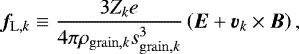$$f_{\text{L},k}\equiv \frac{3Z_{k}e}{4\pi {\rho }_{\text{grain},k}{s}_{\text{grain},k}^3}\left(E+v_k\times B\right),$$(31)

where Z_k is the number of charges on the dust grain k, e = 1.6 × 10⁻²⁰ Abc the electron charge and E is the electric field. The gyration time of a grain is expressed as 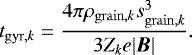$$t_{\text{gyr},k}=\frac{4\pi {\rho }_{\text{grain},k}{s}_{\text{grain},k}^3}{3Z_{k}e\left|B\right|}.$$(32)

A grain subject to a significant Lorentz drag could preferentially couple to the magnetic field rather than the gas. In addition, by controlling the Ohmic, ambipolar, and Hall resistivities (Kunz & Mouschovias 2009), charged grains most likely affect the evolution of the magnetic and electric fields. To compare the magnetic and neutral dragstrength, it is interesting to compare the stopping-to-gyration time ratio also known as the Hall factor Γ_k. In the Epstein regime, this ratio writes 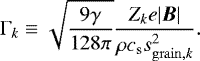$${\Gamma }_k\equiv \sqrt{\frac{9\gamma }{128\pi }}\frac{Z_{k}e\left|B\right|}{\rho c_{\text{s}}{s}_{\text{grain},k}^2}.$$(33)

To model the Hall factor in a collapsing core, we consider a gas with a barotropic equation of state with T_g = 10 K, an adiabatic index γ = 5∕3, and negatively charged grains. The grain charge computation follows Wurster et al. (2016) and is detailed in Appendix C. We use simple assumptions for the magnetic field, stating that $$\left|B\right|=\text{min}\left(B_0{\left(\frac{\rho }{{\rho }_0}\right)}^{2/3},0.1\text{G}\right),$$(34)

where B₀ is the initial magnetic field given by μ, and ρ₀ is the initial core density. The magnetic threshold at 0.1 G is imposed to reproduce the plateau systematically observed when considering ambipolar diffusion Masson et al. (2016), Hennebelle et al. (2016) and Vaytet et al. (2018). One can then show that $${\Gamma }_k=\sqrt{\frac{9\gamma }{128\pi }}\frac{Z_{k}e}{\rho c_{\text{s}}{s}_{\text{grain},k}^2}\text{min}\left(\frac{M_0{}^{1/3}}{\mu {\left(\frac{M_0}{\Phi }\right)}_{\text{c}}}{\left(\frac{4\pi \rho }{3}\right)}^{2/3},0.1\text{G}\right).$$(35)

Figure 21 shows the absolute value of the Hall factor as a function of the density and the grain size. For a wide range of grain sizes, the Hall factor is always much smaller than unity. These grains can therefore be considered neutral at least dynamically. We note that Γ_k is larger than unity for very small grains (s_grain,k ≾ 10⁻⁶ cm). These grains are very well coupled to the gas in the neutral case but, when charged, could experience a strong decoupling with the neutrals. This would occur if the latter were decoupled from the magnetic field, for example, in the nonideal regime. The Lorentz drag might play a crucial role for the dynamics of very small grains in star formation but is probably not very important for the large grains that we observe to decouple in our models. Efforts to study the dynamics of such grains have been made in the past (Guillet et al. 2007; Hopkins & Squire 2018) and should be extended to dusty collapses in future studies. We emphasize that the electromotive term in the Lorentz force applies only to the charged species and not the barycenter and might play a very important role in the decoupling between the charged grains and the neutrals (barycenter) even when Γ_k < 1.

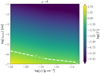Fig. 21 Hall factor as a function of the density and the grain size for μ = 5 for negatively charged grains. The dashed line denotes the equality between the gyration and the stopping time.

7.5 Caveat: coagulation and fragmentation during the collapse

Dust coagulation has been neglected during this study. However, it may significantly affect dust evolution during the collapse as dust decoupling depends on grain size. Following Draine (1985), one can estimate the coagulation timescale t_coag,i,j between two dust phases i and j due to their relative motion within the collapsing clouds as $$t_{\text{coag},i,j}={\left[\frac{3}{4}{\rho }_i\frac{{(s_{\text{grain},i}+s_{\text{grain},j})}^2}{{\rho }_{\text{grain},i}{s}_{\text{grain},i}^3}|v_i-v_j|\right]}^{-1}.$$(36)

Assuming the same density for all the grains, neglecting cumulative back-reaction effects and magnetic fields, and considering an isothermal collapse, differential velocities can be estimated from the diffusion approximation as $$|v_i-v_j|~{\rho }_{\text{grain}}|s_{\text{grain},i}-s_{\text{grain},j}|c_{\text{s}}\frac{|\nabla \rho |}{{\rho }^2}.$$(37)

As said in Sect. 6, the density profile of the free-falling material can be approximated as a power law with an exponent ζ = −2 (Larson 1969). In this case, one obtains at a distance r from the central region $$t_{\text{coag},i,j}={\left[\frac{3\left|\zeta \right|}{4r}{\varepsilon }_i(1+q_{i,j})(1-q_{i,j}^2)c_{\text{s}}\right]}^{-1},$$(38)

where $q_{i,j}\equiv \frac{s_{\text{grain},j}}{s_{\text{grain},i}}$ is the ratio between the grain sizes. In the limit q_i,j ≪ 1, we find $$t_{\text{coag},i,j}~170 \text{kyr}{\left(\frac{{\varepsilon }_j}{{10}^{-2}}\right)}^{-1}\left(\frac{r}{100 \text{AU}}\right){\left(\frac{c_{\text{s}}}{0.19 \text{km}{\text{s}}^{-1}}\right)}^{-1}.$$(39)

Growth induced by the relative dynamics between dust grains is therefore expected to be inefficient during protostellar collapse away from the core but could be non-negligible in the inner regions. At r = 10 AU, t_coag,i,j ~ 17 kyr, which is slightly smaller than the typical free-fall timescale of a prestellar core.

We note that growth could also be enhanced by turbulence, the Brownian motions of dust grains, or focalization due to grain charges (Blum & Wurm 2008). In the case of Brownian motions, for example, assuming that the grain temperature is equal to the gas temperature, the differential velocity for two grains of different mass can be expressed as (Birnstiel et al. 2016) $$|v_i-v_j|=\sqrt{\frac{8k_{\text{B}}{T}_{\text{g}}}{\pi }}\sqrt{\frac{m_{\text{grain},i}+m_{\text{grain},j}}{m_{\text{grain},i}{m}_{\text{grain},j}}}.$$(40)

Therefore, assuming again that q_i,j ≪ 1 the coagulation timescale can be written as $$t_{\text{coag},i,j}={\left[\frac{3}{4}{\rho }_i\frac{1}{{\rho }_{\text{grain},i}{s}_{\text{grain},i}}\sqrt{\frac{8k_{\text{B}}{T}_{\text{g}}}{\pi m_{\text{grain},j}}}\right]}^{-1}.$$(41)

We now consider a region of density 10⁻¹² g cm⁻³ and temperature of 10 K. Assuming s_grain,j = 0.1 μm and s_grain,i = 100 μm, we get t_coag,i,j ~ 240 kyr. We note that, in the case of the Brownian motions, the coagulation timescale depends on the grains size of both species. If we now consider s_grain,j = 0.01 μm, t_coag,i,j ~ 7 kyr.

In short, we are tempted to say that in the presence of large grains, very small grains could be efficiently removed during the collapse in high-density regions. Coagulation should therefore be included in future studies. However, we admit that the presence of such large grains during the early phases of the protostellar collapse is still under debate. It is indeed unclear how these large dust grains can overcome the fragmentation barrier, as the differential velocities between two dust species is typically quite large; for example, up to a few ≈ 0.1km s⁻¹ in the envelope of MMMRN in the case of the two least coupled species. Typically, the velocity above which fragmentation can occur is thought to be about a few times 10 m s⁻¹ (Blum & Wurm 2008) although it could be higher (Yamamoto et al. 2014). Large grains could overcome the fragmentation barrier because the fragmentation timescale is typically equivalent to the coagulation timescale (e.g., Gonzalez et al. 2017). Fragmentation could simply not have the time to occur during the collapse, especially considering the fact that large grains quickly drift toward regions of high density where their drift velocity is typically around a few meters per second. Let us now estimate the typical fragmentation radius r_frag, which corresponds to the distance from the center at which the fragmentation velocity v_frag is equal to the dust drift velocity; it can be obtained by solving $${\rho }_{\text{grain}}{s}_{\text{grain}}{c}_{\text{s}}\frac{|\nabla \rho |}{{\rho }^2}=v_{\text{frag}}.$$(42)

Let us now assume first core formation with a core profile of the type $\rho =\frac{{\rho }_{\mathcal{F}}}{1+{\left(\frac{r}{r_{\mathcal{F}}}\right)}^2}$. We can show that $$r_{\text{frag}}=\frac{1}{2}\frac{r_{\mathcal{F}}^2}{s_{\text{grain}}}\frac{{\rho }_{\mathcal{F}}}{{\rho }_{\text{grain}}}\frac{v_{\text{frag}}}{c_{\text{s}}}.$$(43)

Assuming ${\rho }_{\mathcal{F}}={10}^{-11}\text{g}{\text{cm}}^{-3}$, $r_{\mathcal{F}}=10$AU, ρ_grain = 1 g cm⁻³, s_grain = 160 μm and T_g = 10 K $$\begin{array}{lll}{r}_{\text{frag}}\hfill & =\hfill & 2.5\times {10}^4 \text{AU}{\left(\frac{r_{\mathcal{F}}}{10 \text{AU}}\right)}^2\left(\frac{{\rho }_{\mathcal{F}}}{{10}^{-11}\text{g}{\text{cm}}^{-3}}\right)\left(\frac{c_{\text{s}}}{0.19 \text{km}{\text{s}}^{-1}}\right)\hfill \\ \hfill & \hfill & \left(\frac{v_{\text{frag}}}{10 \text{m}{\text{s}}^{-1}}\right){\left(\frac{s_{\text{grain}}}{160 \mu \text{m}}\right)}^{-1}{\left(\frac{{\rho }_{\text{grain}}}{1 \text{g}{\text{cm}}^{-3}}\right)}^{-1}.\hfill \end{array}$$(44)

The fragmentation radius is significantly larger than the scales that are involved during the first protostellar collapse. We note a quadratic dependency with respect to the first core radius. For a core of size 1 AU, one finds r_frag = 2.5 × 10² AU. Hence, fragmentation may be relevant for small cores and should be investigated in further studies.

8 Conclusion and perspective

In this study, we present the first MULTIGRAIN and nonideal MHD simulations of dusty protostellar collapses using the new dust dynamics solver of RAMSES. We present six DUSTYCOLLAPSE simulations with a simultaneous treatment of ten dust species with different sizes. In these simulations, we investigate the impact of the maximum grain size, the thermal-to-gravitational energy ratio, and the presence of magnetic fields on the dynamics of the DUSTYCOLLAPSE. We summarize below our principal findings:

• 1.

  Small grains with sizes of less than a few tens of microns are strongly coupled to the gas during the protostellar collapse. On the contrary, grains larger than ~100 μm tend to decouple significantly.

• 2.

  When the first hydrostatic core forms, high-density regions – the core, the fragments, the disk, and the pseudo-disk – are enriched in dust by a typical factor of two, whereas low-density regions – the envelope and the outflow – are strongly dust depleted.

• 3.

  Dust is not necessarily a proxy for gas during the collapse. Inferring gas densities from dust is found to potentially lead to extremely large errors (up to ~250%).

• 4.

  A standard MRN grain-size distribution with a maximum grain size of 250 nm is however extremely well preserved during the protostellar collapse in the absence of coagulation.

• 5.

  Dust dynamics is strongly affected by the initial cloud properties. Variations of the dust-to-gas ratio are greatest when the free-fall is long and the initial density is low. An additional decoupling occurs for neutral grains in the presence of magnetic fields because collapse proceeds over longer timescales.

• 6.

  With a semi-analytical model, we show that the dust-ratio varies exponentially with the initial Stokes number during the collapse. More precisely, we show that it can be expressed as ɛ₀ χ^St₀ where χ is a dimensionless function of time and is independent of the dust properties. Fitting the values of χ leads to very good agreement between the semi-analytical model and the measured dust ratios in the range of Stokes numbers considered in our simulations.

• 7.

  Using the calibration of χ with the results of our model, we show that a Stokes number of at least 0.01 is required to enrich the core and the disk in a dust species by a factor of two. Similarly we show that grains with St_0 ≿ 0.027 can potentially be depleted by a factor of two in the envelope after the first core formation.

Dust evolution during the protostellar collapse could have serious consequences on the initial state of protoplanetary disks and the further formation of the planets. In the future, substantial efforts should be made to include the dynamics of charged dust grains during the protostellar collapse because the Lorentz drag cannot necessarily be neglected for small grains. Coagulation and fragmentation of dust grains should also be considered to investigate dust evolution during the star formation process more realistically.

Acknowledgements

First, we thank the referee for providing useful comments and advice that helped us to ameliorate our manuscript. We acknowledge financial support from “Programme National de Physique Stellaire” (PNPS) of CNRS/INSU, CEA and CNES, France. This work was granted access to the HPC resources of CINES (Occigen) under the allocation DARI A0020407247 made by GENCI. Computations were also performed at the Common Computing Facility (CCF) of the LABEX Lyon Institute of Origins (ANR-10-LABX-0066). This work took part under the programs ISM3D and Core2disk of the PSI2 project funded by the IDEX Paris-Saclay, ANR-11-IDEX-0003-02. This project was partly supported by the IDEXLyon project (contract n ANR-16-IDEX-0005) under University of Lyon auspices. The plots were generated using the very efficient Osiris library developed by Neil Vaytet, Tommaso Grassi and Matthias González whom we thank. This project has received funding from the European Union’s Horizon 2020 research and innovation program under the Marie Skłodowska-Curie grant agreement No 823823. We also thank Etienne Jaupart for useful discussions on the theoretical model for the dust enrichment during the collapse.

Appendix A: Impact of velocity regularization

As explained in Sect. 3.5, the simulations of our fiducial model were performed with various values for the maximum gas and dust differential velocity w_cap. We investigated the effect of varying w_cap by performing complementary simulations with w_cap = 0.1, 0.5, 1 and 2 km s⁻¹. We attempted to simulate an additional model with w_cap = 10 km s⁻¹ but this led to numerical instabilities due to unrealistically large dust velocities at the accretion shock, where the diffusion approximation is not valid.

In Fig. A.1, we show a face-one view of the dust ratio at the time of the FHSC formation for these four models. With w_cap = 0.5−2 km s⁻¹ we generally find the same results as in the fiducial case that has w_cap = 1 km s⁻¹. However, having w_cap = 0.1 km s⁻¹ appears to be an overly extreme choice; it indeed suppresses most of the initial dust enrichment that is due to the decoupling between the gas and the dust in the envelope. Having w_cap = 1 km s⁻¹ appeared to be a reasonable choice to cope with time stepping and physical constraints.

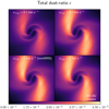Fig. A.1 Fiducial model for various maximum dust differential velocity wcap. Mid-plane view of the total dust ratio at the FHSC formation. (Top-left) wcap = 0.1 km s−1, (top-right) wcap = 0.5 km s−1, (bottom-left)wcap = 1 km s−1, (bottom-right) wcap = 2 km s−1.

Appendix B: Nonlinear dust enrichment: neglecting back-reaction

As stated in Sect. 6, Eq. (25) is valid as long as local dust-ratio variations and the cumulative back-reaction of the dust can be neglected. In this approximation, the dust ratio enrichment increases exponentially with the Stokes number. As pointed out in Sect. 6, we observe deviations from the exponential law in the disk and the envelope in MMMRN, while it is very well verified in the core.

To ascertain whether these deviations are due to back-reaction or not, we perform an additional simulation similar to the fiducial one, but with θ_d,0 = 10⁻⁷ (MMMRNEPS1E-7). For MMMRNEPS1E-7, we expect the back-reaction to be definitely negligible as θ_d,0 ≪ 1.

Figure B.1 shows the dust ratio enrichment as a function of the initial Stokes number for MMMRN (red) and MMMRNEPS1E-7 (pink) in the core, disk, and envelope at t_core + 2 kyr. On top of this, the dust ratio in the disk but at t_core is plotted for MMMRN (gray). As can be seen, the differences between the models at t_core + 2 kyr have similardust-ratio enrichment. This indicates that the cumulative back-reaction of dust is negligible when St_k,0 < 10⁻² and only corrective above that. We are also confident that the mixing between dust-enriched and dust-depleted content, that is, a non-negligible ∇ɛ, are the source of discrepancy between a pure exponential enrichment and the values measured in our models in the disk. We indeed observe very good agreement with the exponential law for MMMRN at t_core. At this timethe disk has just formed from the dense and dust-enriched material of the inner envelope. Later at t_core + 2 kyr, the disk has been accreting material from the envelope that is significantly depleted in large grains which causes a diminution of the average dust enrichment.

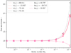Fig. B.1 Semi-analytic and measured dust-ratio enrichment in MMMRN (red) and MMMRNEPS1E-7 (pink) in the core (stars), disk (triangles) and envelope (circles) at tcore + 2 kyr against the initial Stokes number. The lines represent the semi-analytical development using a best fit of χ for the FHSC (dotted), disk (solid), and envelope (dashed), respectively. We display the same information for MMMRN at tcore in the disk (gray).

Appendix C: Charges on dust grains

One can crudely estimate the charges on the grains during the collapse, similarly to Wurster et al. (2016), to compare the relative intensities of the Lorentz and the Epstein drags. For simplicity, we assume that all the grains have the same negative charge Z_d (for all k, Z_k = Z_d) and the ions to have a charge Z_ions = 1. We consider 100 dust bins distributed as an MRN extended to millimeter-sized grains with a dust-to-gas ratio of 1%. Local electroneutrality ensures that $$n_{\text{ions}}-n_{\text{e}}+Z_{\text{d}}{n}_{\text{d}}=0,$$(C.1)

n_ions, n_e and n_d being the number density of the ions, electrons and dust, the latter being given by 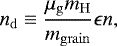$$n_{\text{d}}\equiv \frac{{\mu }_{\text{g}}{m}_{\text{H}}}{m_{\text{grain}}}\varepsilon n,$$(C.2)

where m_grain is the average mass of a dust grain.

Two additional constraints are provided by the evolution equations for the ion and electron charge density (Umebayashi & Nakano 1980; Fujii et al. 2011). Assuming steady state and only considering charge capture by the grains (Keith & Wardle 2014), these equations are 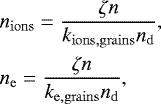$$\begin{array}{l}{n}_{\text{ions}}=\frac{\zeta n}{k_{\text{ions},\text{grains}}{n}_{\text{d}}},\\ n_{\text{e}}=\frac{\zeta n}{k_{\text{e},\text{grains}}{n}_{\text{d}}},\end{array}$$(C.3)

where ζ is the cosmic-ray ionization rate. Similarly to Wurster et al. (2016), we adopt the typical value ζ = 10⁻¹⁷ s⁻¹. We also express k_ions,grains and k_e,grains, the charge capture rates on neutral grains, as in (Fujii et al. 2011) as $$\begin{array}{l}{k}_{\text{ions},\text{grains}}\equiv \pi s_{\text{grain}}^2\sqrt{\frac{8k_{\text{b}}{T}_{\text{g}}}{\pi m_{\text{ions}}}}\left(1-\frac{e^2{Z}_{\text{d}}}{s_{\text{grain}}{k}_{\text{b}}{T}_{\text{g}}}\right),\\ k_{\text{e},\text{grains}}\equiv \pi s_{\text{grain}}^2\sqrt{\frac{8k_{\text{b}}{T}_{\text{g}}}{\pi m_{\text{e}}}}\exp \left[\frac{e^2{Z}_{\text{d}}}{s_{\text{grain}}{k}_{\text{b}}{T}_{\text{g}}}\right],\end{array}$$(C.4)

where s_grain is the average grain size, m_e is the electron mass, and m_ions the ions mass, assumed to be 24.3 proton masses. Using the previous equations, one obtains $$Z_{\text{d}}=\frac{\zeta }{n}{\left(\frac{m_{\text{grain}}}{\varepsilon {\mu }_{\text{g}}{m}_{\text{H}}}\right)}^2\left[\frac{1}{k_{\text{ions},\text{grains}}(Z_{\text{d}})}-\frac{1}{k_{\text{e},\text{grains}}(Z_{\text{d}})}\right],$$(C.5)

which we invert using the Newton-Raphson method to get Z_d.

Appendix D: Distributions

In Table D.1, we provide the initial dust distributions, rounded quantities for the three maximum grain sizes used in our models (the exact calculation can be made using the method presented in Sect. 3.3). Table D.2 shows $<{\Theta }_{\text{d},k}{>}_m$ (in %), the dust-to-gas ratio averaged in mass, along with its corresponding dust enrichment, and the gas mass (in units of M_⊙) for all runs t_core + 2 kyr and all the different objects.

References

All Tables

All Figures

	Fig. 1 Logarithm of the maximum (10th bin) Stokesnumber as a function of the spherical radius for the four models with the largest Stokes numbers at tcore + 2 kyr. Top-left: MMMRN, top-right: MMMRNA0.25, bottom-left: MMMRNMHD, bottom-righ: MMMRNNIMHD.
In the text

Fig. 2 MMMRN test at tcore + 1 kyr and tcore + 2 kyr (tcore =72.84 kyr). Edge-on and mid-plane cuts of the gas and the dust densities for the least coupled species are provided (left and rights respectively). Values of the gas density are indicated by the colorbar at the bottom. Dust densities have been multiplied by a factor 100 to be represented on the same scale. Hence, colors of the gas and the dust maps match when the dust-to-gas ratio equals its initial value 0.01. Dust densityvariations in regions where ɛ0ρd < min(ρg) have voluntarily not been displayed to highlight the enriched regions. These depleted regions are delimited by the dashed gray lines. This choice of colors applies for all density maps in this study. Gas and dust are clearly not perfectly coupled.

In the text

Fig. 3 MMMRN test at tcore + 2 kyr: probability density function (PDF) of the dust ratio enrichment $\log (\overline{\varepsilon })$ for the two most coupled and three least coupled dust species (colored dashed lines) and for all the dust (black line) in the core+fragments (left), the disk (middle), and the envelope (right). Dust is not a good tracer for the gas here and the dust distribution is not uniform in the considered objects.

In the text

Fig. 4 MMMRN test ~ 1 kyr (top), ~2 kyr (middle), and ~4 kyr (bottom) after the first core formation (tcore = 72.84 kyr). Mid-plane view of the total dust ratio (left) and the dust ratio of the least coupled species (right). The colorbar is the same for both figures. The dotted white lines represent the regions where the total (left) or 160 μm grain (right) dust-to-gas ratio is at its initial value, which can also be regarded as a dust enrichment line.

In the text

	Fig. 5 MMMRN test at tcore + 1 kyr (tcore =72.84 kyr). Mid-plane view of the gas pressure (up-close). The white arrows represent the direction of the differential velocity w10.
In the text

Fig. 6 MMMRN test. Volume averaged total dust-to-gas ratio enrichment as a function of time for different density thresholds.The FHSC formation can be identified by the dotted vertical blue line while fragmentation occurs during a time delimited by the green area. We observe a slow decrease of the dust-to-gas ratio at low density which gives rise to an enrichment of high-density regions. Cores and fragments at ρ > 10−11 g cm−3 are formed in a dust-rich environment. The dust-to-gas ratio is almost constant for ρ > 10−11 g cm−3 because the increase of temperature due to the adiabatic contraction strengthens the coupling between the gas and the dust.

In the text

	Fig. 7 MRN test at tcore + 2 kyr (tcore =73.6 kyr). Edge-on (top) and mid-plane (bottom) cuts of the gas density (left) and dust density of the least coupled species (right). The two maps are almost indistinguishable due to the very strong coupling between gas and all dust species.
In the text

	Fig. 8 MRN test at tcore + 2 kyr. Probability density function (PDF) of the total dust ratio enrichment $\log (\overline{\varepsilon })$ in the core and the fragments, the disk, and the envelope. Dust is a very good tracer of mass here and the dust distribution is almost uniform in the objects considered.
In the text

	Fig. 9 100MICMRN test at tcore + 2 kyr. Probability density function of the total dust ratio enrichment $\log (\overline{\varepsilon })$ in the core and the fragments, the disk, and the envelope. Dust is a relatively good tracer of gas although significant variations of the dust-to-gas ratio are observed.
In the text

	Fig. 10 MMMRNA0.25 test at tcore + 2 kyr (tcore =23 kyr). Edge-on (top) and mid-plane (bottom) cuts of the gas density (left) and dust density of the least coupled species (right). Dust has less time to significantly decouple from the gas than in the MMMRN case. A strong dust depletion is observed in the envelope.
In the text

	Fig. 11 MMMRNA0.25 test at tcore + 2 kyr. Probability density function of the total dust ratio enrichment $\log (\overline{\varepsilon })$ in the core+fragments, the disk, and the envelope. Dust is a relatively good tracer for gas in the dense object although a notable depletion is observed in the envelope.
In the text

	Fig. 12 MMMRNMHD at tcore + 2 kyr (tcore =81.1 kyr). Edge-on (top) and mid-plane (bottom) cuts of the gas density (left) and dust density of the least coupled species (right). Dust is significantly decoupled from the gas and concentrates in the high-density regions such as the core, the disk, the pseudo-disk,and the inner regions of the outflow.
In the text

	Fig. 13 MMMRNNIMHD at tcore + 2 kyr (tcore =81.1 kyr). Edge-on (top) and mid-plane (bottom) cuts of the gas density (left) and dust density of the least coupled species (right). As in the ideal case, dust is significantly decoupled from the gas and concentrates in the high-density regions such as the core, the disk, the pseudo-disk, and the inner regions of the outflow.
In the text

	Fig. 14 MMMRNMHD test at tcore + 2 kyr. Probability density function of the dust ratio enrichment $\log (\overline{\varepsilon })$ in the core (blue), the disk (green), the pseudo-disk (purple), the outflow (orange) and the envelope (red). Dust is not a good tracer of gas here and the dust distribution is not uniform in the considered objects.
In the text

	Fig. 15 MMMRNNIMHD test at tcore + 2 kyr. Probability density function of the dust ratio enrichment $\log (\overline{\varepsilon })$ in the core (blue), the disk (green), the pseudo-disk (purple), the outflow (orange) and the envelope (red). Dust is not a good tracer of gas here and the dust distribution is not uniform in the considered objects.
In the text

Fig. 16 All the models at tcore + 2 kyr. The dust-to-gas ratio enrichment averaged in mass is shown as a function of grain size for all the objects. Grains with sizes smaller than 10−4 cm are almost always perfectly coupled with the gas. For larger grain sizes, the enrichment is model dependent. Grains with typical sizes larger than 10−3 cm decouple from the gas. Dense objects such as the fragments $\mathcal{F}$ or the disk $\mathcal{D}$ and pseudo-disk $\mathcal{P}$ are enriched in dust. Low-density objects such as the envelope $\mathcal{E}$ or the outflows $\mathcal{O}$ are depletedin dust. Magnetized models exhibit the strongest decoupling between the gas and the dust.

In the text

	Fig. 17 mmMRNmhd. Edge-on view of the relative variations of the dust ratio at four different times for the 47 μm (left) 160 μm grains (right). The magenta arrows represent the differential velocity with the barycenter. Regions that are dust depleted by more than two orders of magnitude are not displayed (black background).
In the text

	Fig. 18 MMMRNMHD at tcore + 2 kyr. Edge-on view of the total column density log(Σ) (top), the total error Err (middle) and the error when using the largest grains only – 160 μm in this case (bottom).
In the text

Fig. 19 Semi-analytic and measured enrichment in our hydrodynamical models (MRN excluded) against the initial Stokes number. The lines represent the semi-analytical development using a best fit of χ for the FHSC (dotted), disk (solid), and envelope (dashed), respectively. The extreme values of the enrichment given by our toy model are delimited by the blue areas. The color coding and choice of markers is the same as in Fig. 16.

In the text

Fig. 20 Schematic view of a dusty protostellar collapse. Blue regions are dust depleted and red regions are dust enriched. Typically, the outer regions of the envelope are depleted. The outflow, only observed in magnetic runs, is enriched on its surface and depleted elsewhere. Dense regions such as the core and fragments $\mathcal{F}$ (the fragments are observed only in the hydrodynamical case), the pseudo-disk $\mathcal{P}$ (only in magnetic runs), and the disk $\mathcal{D}$ are generally enriched. The strength of dust decoupling depends on the initial choice of parameters such as the maximum grain size, the thermal-to-gravitational energy ratio, or the presence of a magnetic field. This view of a dusty protostellar collapse is simplified and provides only a global sketch of the evolution.

In the text

	Fig. 21 Hall factor as a function of the density and the grain size for μ = 5 for negatively charged grains. The dashed line denotes the equality between the gyration and the stopping time.
In the text

	Fig. A.1 Fiducial model for various maximum dust differential velocity wcap. Mid-plane view of the total dust ratio at the FHSC formation. (Top-left) wcap = 0.1 km s−1, (top-right) wcap = 0.5 km s−1, (bottom-left)wcap = 1 km s−1, (bottom-right) wcap = 2 km s−1.
In the text

Fig. B.1 Semi-analytic and measured dust-ratio enrichment in MMMRN (red) and MMMRNEPS1E-7 (pink) in the core (stars), disk (triangles) and envelope (circles) at tcore + 2 kyr against the initial Stokes number. The lines represent the semi-analytical development using a best fit of χ for the FHSC (dotted), disk (solid), and envelope (dashed), respectively. We display the same information for MMMRN at tcore in the disk (gray).

In the text

References

- Allen, A., Shu, F. H., & Li, Z.-Y. 2003, ApJ, 599, 351 [NASA ADS] [CrossRef] [Google Scholar]
- Andrews, S. M., Wilner, D. J., Hughes, A. M., Qi, C., & Dullemond, C. P. 2010, ApJ, 723, 1241 [NASA ADS] [CrossRef] [Google Scholar]
- Bate, M. R., & Lorén-Aguilar, P. 2017, MNRAS, 465, 1089 [NASA ADS] [CrossRef] [Google Scholar]
- Belloche, A. 2013, EAS Pub. Ser., 62, 25 [CrossRef] [EDP Sciences] [Google Scholar]
- Berger, M. J., & Oliger, J. 1984, J. Comput. Phys., 53, 484 [NASA ADS] [CrossRef] [MathSciNet] [Google Scholar]
- Birnstiel, T., Dullemond, C. P., & Brauer, F. 2009, A&A, 503, L5 [NASA ADS] [CrossRef] [EDP Sciences] [Google Scholar]
- Birnstiel, T., Fang, M., & Johansen, A. 2016, Space Sci. Rev., 205, 41 [NASA ADS] [CrossRef] [Google Scholar]
- Blum, J., & Wurm, G. 2008, ARA&A, 46, 21 [Google Scholar]
- Bodenheimer, P. 1995, ARA&A, 33, 199 [NASA ADS] [CrossRef] [Google Scholar]
- Boss, A. P., & Bodenheimer, P. 1979, ApJ, 234, 289 [NASA ADS] [CrossRef] [Google Scholar]
- Brauer, F., Dullemond, C. P., & Henning, T. 2008, A&A, 480, 859 [NASA ADS] [CrossRef] [EDP Sciences] [Google Scholar]
- Commerçon, B., Hennebelle, P., Audit, E., Chabrier, G., & Teyssier, R. 2008, A&A, 482, 371 [NASA ADS] [CrossRef] [EDP Sciences] [Google Scholar]
- Commerçon, B., Hennebelle, P., Audit, E., Chabrier, G., & Teyssier, R. 2010, A&A, 510, L3 [NASA ADS] [CrossRef] [EDP Sciences] [Google Scholar]
- Commerçon, B., Hennebelle, P., & Henning, T. 2011a, ApJ, 742, L9 [NASA ADS] [CrossRef] [Google Scholar]
- Commerçon, B., Teyssier, R., Audit, E., Hennebelle, P., & Chabrier, G. 2011b, A&A, 529, A35 [NASA ADS] [CrossRef] [EDP Sciences] [Google Scholar]
- Commerçon, B., Debout, V., & Teyssier, R. 2014, A&A, 563, A11 [NASA ADS] [CrossRef] [EDP Sciences] [Google Scholar]
- Dipierro, G., & Laibe, G. 2017, MNRAS, 469, 1932 [NASA ADS] [CrossRef] [Google Scholar]
- Dipierro, G., Laibe, G., Alexander, R., & Hutchison, M. 2018, MNRAS, 479, 4187 [NASA ADS] [CrossRef] [Google Scholar]
- Draine, B. T. 1985, in Protostars and Planets II, eds. D. C. Black, & M. S. Matthews (Tucson, AZ: University of Arizona Press), 621 [Google Scholar]
- Draine, B. T. 2004, in The Cold Universe (Berlin: Springer), 213 [NASA ADS] [CrossRef] [Google Scholar]
- Dra̧żkowska, J., Alibert, Y., & Moore, B. 2016, A&A, 594, A105 [NASA ADS] [CrossRef] [EDP Sciences] [Google Scholar]
- Dubois, Y., & Commerçon B. 2016, A&A, 585, A138 [NASA ADS] [CrossRef] [EDP Sciences] [Google Scholar]
- Dubois, Y., Commerçon, B., Marcowith, A. r., & Brahimi, L. 2019, A&A, 631, A121 [CrossRef] [EDP Sciences] [Google Scholar]
- Elbakyan, V. G., Johansen, A., Lambrechts, M., Akimkin, V., & Vorobyov, E. I. 2020, A&A, 637, A5 [CrossRef] [EDP Sciences] [Google Scholar]
- Epstein, P. S. 1924, Phys. Rev., 23, 710 [NASA ADS] [CrossRef] [Google Scholar]
- Fromang, S., & Papaloizou, J. 2006, A&A, 452, 751 [NASA ADS] [CrossRef] [EDP Sciences] [Google Scholar]
- Fromang, S., Hennebelle, P., & Teyssier, R. 2006, A&A, 457, 371 [NASA ADS] [CrossRef] [EDP Sciences] [Google Scholar]
- Fujii, Y. I., Okuzumi, S., & Inutsuka, S.-i. 2011, ApJ, 743, 53 [NASA ADS] [CrossRef] [Google Scholar]
- Galametz, M., Maury, A. J., Valdivia, V., et al. 2019, A&A, 632, A5 [NASA ADS] [CrossRef] [EDP Sciences] [Google Scholar]
- Galli, D., & Shu, F. H. 1993, ApJ, 417, 220 [NASA ADS] [CrossRef] [Google Scholar]
- Godunov, S. K. 1959, Mat. Sb., 47, 271 [Google Scholar]
- González, M., Vaytet, N., Commerçon, B., & Masson, J. 2015, A&A, 578, A12 [NASA ADS] [CrossRef] [EDP Sciences] [Google Scholar]
- Gonzalez, J.-F., Laibe, G., & Maddison, S. T. 2017, MNRAS, 467, 1984 [NASA ADS] [Google Scholar]
- Gould, R. J., & Salpeter, E. E. 1963, ApJ, 138, 393 [NASA ADS] [CrossRef] [Google Scholar]
- Guillet, V., Pineau Des Forêts, G., & Jones, A. P. 2007, A&A, 476, 263 [NASA ADS] [CrossRef] [EDP Sciences] [Google Scholar]
- Hennebelle, P., & Fromang, S. 2008, A&A, 477, 9 [NASA ADS] [CrossRef] [EDP Sciences] [Google Scholar]
- Hennebelle, P., Commerçon, B., Chabrier, G., & Marchand, P. 2016, ApJ, 830, L8 [NASA ADS] [CrossRef] [Google Scholar]
- Hennebelle, P., Commerçon, B., Lee, Y.-N., & Charnoz, S. 2020, A&A, 635, A67 [CrossRef] [EDP Sciences] [Google Scholar]
- Hincelin, U., Commerçon, B., Wakelam, V., et al. 2016, ApJ, 822, 12 [NASA ADS] [CrossRef] [Google Scholar]
- Hopkins, P. F., & Squire, J. 2018, MNRAS, 479, 4681 [NASA ADS] [CrossRef] [Google Scholar]
- Hutchison, M., Price, D. J., & Laibe, G. 2018, MNRAS, 476, 2186 [NASA ADS] [CrossRef] [Google Scholar]
- Jaupart, E., & Laibe, G. 2020, MNRAS, 492, 4591 [CrossRef] [Google Scholar]
- Johansen, A., Oishi, J. S., Mac Low, M.-M., et al. 2007, Nature, 448, 1022 [Google Scholar]
- Johansen, A., Youdin, A., & Mac Low M.-M. 2009, ApJ, 704, L75 [NASA ADS] [CrossRef] [Google Scholar]
- Joos, M., Hennebelle, P., & Ciardi, A. 2012, A&A, 543, A128 [NASA ADS] [CrossRef] [EDP Sciences] [Google Scholar]
- Kanagawa, K. D., Ueda, T., Muto, T., & Okuzumi, S. 2017, ApJ, 844, 142 [NASA ADS] [CrossRef] [Google Scholar]
- Kataoka, A., Muto, T., Momose, M., et al. 2015, ApJ, 809, 78 [NASA ADS] [CrossRef] [Google Scholar]
- Kataoka, A., Tsukagoshi, T., Momose, M., et al. 2016, ApJ, 831, L12 [NASA ADS] [CrossRef] [Google Scholar]
- Keith, S. L., & Wardle, M. 2014, MNRAS, 440, 89 [NASA ADS] [CrossRef] [Google Scholar]
- Krapp, L., Benítez-Llambay, P., Gressel, O., & Pessah, M. E. 2019, ApJ, 878, L30 [NASA ADS] [CrossRef] [Google Scholar]
- Kunz, M. W., & Mouschovias, T. C. 2009, ApJ, 693, 1895 [NASA ADS] [CrossRef] [Google Scholar]
- Kwok, S. 1975, ApJ, 198, 583 [NASA ADS] [CrossRef] [Google Scholar]
- Laibe, G. 2014, MNRAS, 437, 3037 [NASA ADS] [CrossRef] [Google Scholar]
- Laibe, G., & Price, D. J. 2014a, MNRAS, 440, 2136 [NASA ADS] [CrossRef] [Google Scholar]
- Laibe, G., & Price, D. J. 2014b, MNRAS, 440, 2147 [NASA ADS] [CrossRef] [Google Scholar]
- Laibe, G., & Price, D. J. 2014c, MNRAS, 444, 1940 [NASA ADS] [CrossRef] [Google Scholar]
- Larson, R. B. 1969, MNRAS, 145, 271 [NASA ADS] [CrossRef] [Google Scholar]
- Lebreuilly, U., Commerçon, B., & Laibe, G. 2019, A&A, 626, A96 [NASA ADS] [CrossRef] [EDP Sciences] [Google Scholar]
- Lin, M.-K. 2019, MNRAS, 485, 5221 [NASA ADS] [CrossRef] [Google Scholar]
- Lovascio, F., & Paardekooper, S.-J. 2019, MNRAS, 488, 5290 [CrossRef] [Google Scholar]
- Machida, M. N., Inutsuka, S.-i., & Matsumoto, T. 2014, MNRAS, 438, 2278 [NASA ADS] [CrossRef] [Google Scholar]
- Marchand, P., Masson, J., Chabrier, G., et al. 2016, A&A, 592, A18 [NASA ADS] [CrossRef] [EDP Sciences] [Google Scholar]
- Marchand, P., Commerçon, B., & Chabrier, G. 2018, A&A, 619, A37 [NASA ADS] [CrossRef] [EDP Sciences] [Google Scholar]
- Marchand, P., Tomida, K., Commerçon, B., & Chabrier, G. 2019, A&A, 631, A66 [CrossRef] [EDP Sciences] [Google Scholar]
- Masson, J., Teyssier, R., Mulet-Marquis, C., Hennebelle, P., & Chabrier, G. 2012, ApJS, 201, 24 [NASA ADS] [CrossRef] [Google Scholar]
- Masson, J., Chabrier, G., Hennebelle, P., Vaytet, N., & Commerçon, B. 2016, A&A, 587, A32 [NASA ADS] [CrossRef] [EDP Sciences] [Google Scholar]
- Mathis, J. S., Rumpl, W., & Nordsieck, K. H. 1977, ApJ, 217, 425 [NASA ADS] [CrossRef] [Google Scholar]
- McKee, C. F., & Ostriker, E. C. 2007, ARA&A, 45, 565 [NASA ADS] [CrossRef] [Google Scholar]
- Mignon-Risse, R., González, M., Commerçon, B., & Rosdahl, J. 2020, A&A, 635, A42 [CrossRef] [EDP Sciences] [Google Scholar]
- Miyoshi, T., & Kusano, K. 2005, J. Comput. Phys., 208, 315 [NASA ADS] [CrossRef] [Google Scholar]
- Mouschovias, T. C., & Spitzer, L. J. 1976, ApJ, 210, 326 [NASA ADS] [CrossRef] [Google Scholar]
- Pagani, L., Steinacker, J., Bacmann, A., Stutz, A., & Henning, T. 2010, Science, 329, 1622 [NASA ADS] [CrossRef] [PubMed] [Google Scholar]
- Pohl, A., Kataoka, A., Pinilla, P., et al. 2016, A&A, 593, A12 [NASA ADS] [CrossRef] [EDP Sciences] [Google Scholar]
- Price, D. J., & Bate, M. R. 2007, Ap&SS, 311, 75 [NASA ADS] [CrossRef] [Google Scholar]
- Price, D. J., & Laibe, G. 2015, MNRAS, 454, 2320 [NASA ADS] [CrossRef] [Google Scholar]
- Roe, P. L. 1986, Ann. Rev. Fluid Mech., 18, 337 [NASA ADS] [CrossRef] [Google Scholar]
- Rosdahl, J., & Teyssier, R. 2015, MNRAS, 449, 4380 [NASA ADS] [CrossRef] [Google Scholar]
- Rosdahl, J., Blaizot, J., Aubert, D., Stranex, T., & Teyssier, R. 2013, MNRAS, 436, 2188 [NASA ADS] [CrossRef] [Google Scholar]
- Sadavoy, S. I., Myers, P. C., Stephens, I. W., et al. 2018a, ApJ, 859, 165 [NASA ADS] [CrossRef] [Google Scholar]
- Sadavoy, S. I., Myers, P. C., Stephens, I. W., et al. 2018b, ApJ, 869, 115 [NASA ADS] [CrossRef] [Google Scholar]
- Sadavoy, S. I., Stephens, I. W., Myers, P. C., et al. 2019, ApJS, 245, 2 [NASA ADS] [CrossRef] [Google Scholar]
- Teyssier, R. 2002, A&A, 385, 337 [NASA ADS] [CrossRef] [EDP Sciences] [Google Scholar]
- Teyssier, R., Fromang, S., & Dormy, E. 2006, J. Comput. Phys., 218, 44 [NASA ADS] [CrossRef] [Google Scholar]
- Tomida, K., Okuzumi, S., & Machida, M. N. 2015, ApJ, 801, 117 [NASA ADS] [CrossRef] [Google Scholar]
- Truelove, J. K., Klein, R. I., McKee, C. F., et al. 1997, ApJ, 489, L179 [NASA ADS] [CrossRef] [Google Scholar]
- Tychoniec, Ł., Manara, C. F., Rosotti, G. P., et al. 2020, A&A, 640, A19 [CrossRef] [EDP Sciences] [Google Scholar]
- Umebayashi, T., & Nakano, T. 1980, PASJ, 32, 405 [NASA ADS] [Google Scholar]
- Umebayashi, T., & Nakano, T. 1990, MNRAS, 243, 103 [NASA ADS] [CrossRef] [Google Scholar]
- Valdivia, V., Maury, A., Brauer, R., et al. 2019, MNRAS, 488, 4897 [NASA ADS] [CrossRef] [Google Scholar]
- van Leer B. 1974, J. Comput. Phys., 14, 361 [NASA ADS] [CrossRef] [Google Scholar]
- Vaytet, N., Commerçon, B., Masson, J., González, M., & Chabrier, G. 2018, A&A, 615, A5 [NASA ADS] [CrossRef] [EDP Sciences] [Google Scholar]
- Vorobyov, E. I., & Elbakyan, V. G. 2019, A&A, 631, A1 [NASA ADS] [CrossRef] [EDP Sciences] [Google Scholar]
- Vorobyov, E. I., Skliarevskii, A. M., Elbakyan, V. G., et al. 2019, A&A, 627, A154 [NASA ADS] [CrossRef] [EDP Sciences] [Google Scholar]
- Whitworth, A. P., & Clarke, C. J. 1997, MNRAS, 291, 578 [NASA ADS] [Google Scholar]
- Wurster, J., Price, D. J., & Bate, M. R. 2016, MNRAS, 457, 1037 [NASA ADS] [CrossRef] [Google Scholar]
- Wurster, J., Bate, M. R., & Price, D. J. 2019, MNRAS, 489, 1719 [NASA ADS] [CrossRef] [Google Scholar]
- Yamamoto, T., Kadono, T., & Wada, K. 2014, ApJ, 783, L36 [NASA ADS] [CrossRef] [Google Scholar]
- Zhao, B., Caselli, P., Li, Z.-Y., et al. 2016, MNRAS, 460, 2050 [Google Scholar]
Distinct from the dust density ρk.
All Tables
Syllabus of the different simulations, with the thermal-to-gravitational energy ratios α, and the maximum grain sizes Smax.
Mass-averaged dust-to-gas ratio (in %) and gas mass (in units of M⊙) for all runs tcore + 2 kyr and all the objects;