| Issue |
A&A
Volume 641, September 2020
|
|
|---|---|---|
| Article Number | A118 | |
| Number of page(s) | 26 | |
| Section | Cosmology (including clusters of galaxies) | |
| DOI | https://doi.org/10.1051/0004-6361/202038133 | |
| Published online | 18 September 2020 | |
The MUSE Hubble Ultra Deep Field Survey
XV. The mean rest-UV spectra of Lyα emitters at z > 3⋆,⋆⋆
1
SISSA, Via Bonomea 265, 34136 Trieste, Italy
2
INAF – Osservatorio di Astrofisica e Scienza dello Spazio di Bologna, Via P. Gobetti 93/3, 40129 Bologna, Italy
e-mail: anna.feltre@inaf.it
3
Leiden Observatory, Leiden University, PO Box 9513, 2300 RA Leiden, The Netherlands
4
Univ Lyon, Univ Lyon1, Ens de Lyon, CNRS, Centre de Recherche Astrophysique de Lyon UMR5574, 69230 Saint-Genis-Laval, France
5
Department of Earth and Space Sciences, Indian Institute of Space Science & Technology, Thiruvananthapuram 695547, India
6
Observatoire de Genève, Universite de Genève, 51 Ch. des Maillettes, 1290 Versoix, Switzerland
7
Leibniz-Institut für Astrophysik Potsdam (AIP), An der Sternwarte 16, 14482 Potsdam, Germany
8
Tomonaga Center for the History of the Universe (TCHoU), Faculty of Pure and Applied Sciences, University of Tsukuba, Tsukuba, Ibaraki 305-8571, Japan
9
Instituto de Astrofísica e Cîencias do Espaço, Universidade do Porto, CAUP, Rua das Estrelas, 4150-762 Porto, Portugal
10
Department of Physics, ETH Zürich, Wolfgang-Pauli-Strasse 27, 8093 Zürich, Switzerland
11
Hiroshima Astrophysical Science Center, Hiroshima University, 1-3-1 Kagamiyama, Higashi-Hiroshima, Hiroshima 739-8526, Japan
12
Institut für Astrophysik, Universität Göttingen, Friedrich-Hund Platz 1, 37077 Göttingen, Germany
13
Centre for Astrophysics and Supercomputing, Swinburne University of Technology, Hawthorn, Victoria 3122, Australia
Received:
9
April
2020
Accepted:
1
July
2020
We investigated the ultraviolet (UV) spectral properties of faint Lyman-α emitters (LAEs) in the redshift range 2.9 ≤ z ≤ 4.6, and we provide material to prepare future observations of the faint Universe. We used data from the MUSE Hubble Ultra Deep Survey to construct mean rest-frame spectra of continuum-faint (median MUV of −18 and down to MUV of −16), low stellar mass (median value of 108.4 M⊙ and down to 107 M⊙) LAEs at redshift z ≳ 3. We computed various averaged spectra of LAEs, subsampled on the basis of their observational (e.g., Lyα strength, UV magnitude and spectral slope) and physical (e.g., stellar mass and star-formation rate) properties. We searched for UV spectral features other than Lyα, such as higher ionization nebular emission lines and absorption features. We successfully observed the O III]λ1666 and [C III]λ1907+C III]λ1909 collisionally excited emission lines and the He IIλ1640 recombination feature, as well as the resonant C IVλλ1548,1551 doublet either in emission or P-Cygni. We compared the observed spectral properties of the different mean spectra and find the emission lines to vary with the observational and physical properties of the LAEs. In particular, the mean spectra of LAEs with larger Lyα equivalent widths, fainter UV magnitudes, bluer UV spectral slopes, and lower stellar masses show the strongest nebular emission. The line ratios of these lines are similar to those measured in the spectra of local metal-poor galaxies, while their equivalent widths are weaker compared to the handful of extreme values detected in individual spectra of z > 2 galaxies. This suggests that weak UV features are likely ubiquitous in high z, low-mass, and faint LAEs. We publicly released the stacked spectra, as they can serve as empirical templates for the design of future observations, such as those with the James Webb Space Telescope and the Extremely Large Telescope.
Key words: galaxies: evolution / galaxies: high-redshift / ISM: lines and bands / ultraviolet: ISM / ultraviolet: galaxies
The average spectra computed in this work are only available at the CDS via anonymous ftp to cdsarc.u-strasbg.fr (130.79.128.5) or via http://cdsarc.u-strasbg.fr/viz-bin/cat/J/A+A/641/A118
© ESO 2020
1. Introduction
Ultraviolet (UV) line-emitting galaxies (at low and high redshift) are receiving a great deal of attention, as they are possible analogs of the faint, low-mass but numerous, distant star-forming galaxies, which are considered the best candidates to provide the hydrogren-ionizing budget to sustain the cosmic reionization down to z ≈ 6 (e.g., Robertson et al. 2015; Bouwens et al. 2016; Finkelstein et al. 2019). The rest-frame UV (λ < 3200 Å) is rich in high-ionization metal lines, for example, [C III]λ1907+C III]λ1909, C IVλ1550, and N Vλ1240, which provide additional information to the rest-optical lines commonly explored to understand the nature of ionizing sources (e.g., Steidel et al. 2016; Senchyna et al. 2017; Topping et al. 2020). Spectral features, in absorption or in emission, provide valuable clues concerning the properties of the stellar populations of galaxies and the physical conditions in their interstellar medium (ISM). While the exploitation of strong rest-optical emission lines for statistical studies of the ionized properties of galaxies is limited to z ≤ 3, current optical and near-infrared ground-based spectrographs (e.g., the Multi Unit Spectroscopic Explorer, MUSE, and X-shooter on the ESO-Very Large Telescope and MOSFIRE of the Keck Observatory) are now providing high-quality rest-UV spectra for targeted samples of galaxies at earlier epochs (from z ≈ 3 out to z ≈ 6 − 7).
A fast-growing number of observational studies of z ≳ 2 galaxies present spectra showing strong UV emission features, in addition to the Lyα line. While the detection of multiple UV emission lines on single spectra mainly relies on measurements performed on gravitationally lensed sources (e.g., Stark et al. 2015a; Berg et al. 2018), large deep surveys, such as VUDS (Le Fèvre et al. 2015) and VANDELS (McLure et al. 2018; Pentericci et al. 2018), have just enabled the assembly of non-lensed samples of UV line-emitting galaxies at z ≈ 2 − 4 (e.g., Amorín et al. 2017; Nakajima et al. 2018a; Le Fèvre et al. 2019; Marchi et al. 2019). High-ionization UV nebular emission lines (e.g., C IVλ1550 and He IIλ1640) have been identified in the spectra of young galaxies at high redshift, from z ≈ 2 up to z ≈ 7 (e.g., Stark et al. 2014, 2015a; Mainali et al. 2017; Berg et al. 2018; Nanayakkara et al. 2019; Vanzella et al. 2010, 2016, 2017, 2020), highlighting the central role of young (≤10 Myr) and massive stars in contributing to the spectral energy distribution (SED) of high-z galaxies, and triggering interest in the ionizing properties of these extreme line emitters. These observations challenge current stellar population synthesis models, as they do not predict hard-enough ionizing radiation to account for the strong He II emission observed in local metal-poor galaxies and z > 2 line-emitting galaxies (e.g., Senchyna et al. 2017; Nanayakkara et al. 2019; Plat et al. 2019).
Obtaining individual high signal-to-noise ratio (S/N) detections of multiple UV lines (other than Lyα) at high z is extremely challenging with current instrumentation, and a standard procedure for studying spectral features too faint to be detected in single spectra is spectral stacking, which provides higher S/N data by co-adding individual lower S/N spectra (e.g., Shapley et al. 2003; Steidel et al. 2010, 2016; Berry et al. 2012; Jones et al. 2012; Rigby et al. 2018; Nakajima et al. 2018b; Pahl et al. 2020; Khusanova et al. 2020; Thomas et al. 2020; Trainor et al. 2019). By splitting ∼1000 Lyman-break galaxies (LBGs) into subsamples based on Lyαλ1216 (hereafter Lyα) equivalent width (EW), UV spectral slope, and UV magnitude, Shapley et al. (2003) studied how the spectral properties of the composite spectra of each subsample depend on other galaxy properties. Berry et al. (2012) and Jones et al. (2012) performed similar analyses on ≈80 UV-bright star-forming galaxies at 2.0 < z < 3.5 and on ≈80 LBGs in the range 3 < z < 7, respectively. One of the main outcomes from these works is that galaxies with stronger Lyα emission show bluer UV continuum slopes, lower stellar masses, and spectra with weaker low-ionization absorption-line profiles and more prominent nebular emission lines. More recently, Pahl et al. (2020) computed stacked spectra by grouping a sample of 375 star-forming galaxies at 4 < z < 5.5 in different bins of Lyα EW and found a decrease in the low-ionization absorption-line strength with increasing EW of Lyα emission up to z ≈ 5, confirming previous trends. Rigby et al. (2018) publicly released the composite spectra of 14 highly magnified star-forming galaxies at 1.6 < z < 2.3. They are extremely rich in absorption and nebular emission features and are to be used as diagnostics of the physical properties of the stellar population, the physical conditions of ionized gas, and outflowing winds within these galaxies. Nakajima et al. (2018b) studied the nebular emission features of ∼100 Lyman-alpha emitters (LAEs) at z ≈ 3.1, confirming earlier suggestions of a correlation between the strength of Lyα and C III] emission (Shapley et al. 2003; Stark et al. 2014) and finding similar trends with the UV luminosities and colors. The results from Nakajima et al. (2018b) support earlier suggestions that LAEs have a significantly larger ionizing production efficiency (ξion) than LBGs (see also Lam et al. 2019). Recently, Saxena et al. (2020) presented the stacked spectra of He II emitters at z ≈ 2.5 − 5.0, identified in the deep VANDELS ESO public spectroscopic survey (McLure et al. 2018; Pentericci et al. 2018), finding no significant difference between galaxies with and without He II emission in terms of stellar masses, star formation rates (SFRs) and rest-frame UV magnitudes.
All of these studies rely implicitly on pre-selections that may not result in a sample that is representative of the overall population. The Multi-Unit Spectroscopic Explorer (MUSE; Bacon et al. 2010) on the Very Large Telescope (VLT), however, has recently enabled the detection and analysis of un-targeted samples of LAEs at 2.9 < z < 6.7 (e.g., Bacon et al. 2015; Wisotzki et al. 2016; Leclercq et al. 2017; Hashimoto et al. 2017a; Drake et al. 2017; Maseda et al. 2018, 2020; Marino et al. 2018), that is, selecting galaxies only on their Lyα emission line. In particular, the MUSE Hubble Ultra Deep Field (HUDF) Survey (Bacon et al. 2017) uncovers an unprecedented number of the UV faint (MUV at 1500 Å down to −16), low stellar mass (down to ∼107 M⊙) LAEs at z > 3, reaching UV luminosities (and stellar masses) two orders of magnitude fainter (smaller) than previous studies. A systematic analysis of how the UV spectral features of these faint and low-mass LAEs depends on the observed and physical properties of galaxies and how they compare with those observed in brighter and more massive sources is missing from the literature.
In this work, we present unweighted mean spectra of the MUSE HUDF LAEs grouped in subsamples on the basis of observational (e.g., Lyα strengths and EW, UV magnitude, and UV spectral slopes) and physical (e.g., stellar mass, SFR) galaxy properties. The aim of this paper is to study variations of the spectral properties among the different LAE subsamples, with a particular focus on nebular line emission. The stacked spectra are publicly available together with this paper and can serve as empirical templates for the design of future observations (e.g., those with the JWST and the ELT).
The spectroscopic dataset is described in Sect. 2, and the stacking procedure in Sect. 3. Section 4 illustrates the different mean spectra and their spectral properties, with particular focus on nebular emission lines such as He IIλ1640, O III]λλ1661,1666, [Si III]λ1883+Si III]λ1892, and [C III]λ1907+C III]λ1909, and the C IVλλ1548,1551 resonant doublet. The dependencies of these features on the galaxy properties, and a comparison with the literature are discussed in Sect. 5, followed by the conclusions in Sect. 6. Throughout the paper, we use the AB flux normalization (Oke & Gunn 1983), and we adopt the cosmological parameters from Planck Collaboration XIII (2016), (ΩM, ΩΛ, H0) = (0.308, 0.692, 67.81).
2. Dataset
2.1. MUSE HUDF Survey and sample selection
We made use of spectroscopic observations from the MUSE HUDF Survey (Bacon et al. 2017), which consists of a mosaic of nine pointings (∼3′×3′) with 10-hour exposure (mosaic) in the HUDF and an additional single deeper exposure of 31 h (udf-10) within the same region. We opted for an upgraded version of the mosaic and udf-10 datacubes (version 1.0), which, compared to version 0.42 used in Bacon et al. (2017), is created with an enhanced data reduction process resulting in an improved sky subtraction and S/N of the extracted spectra (Bacon et al., in prep.).
We used the redshift measurements from the first MUSE HUDF Survey Data Release (DR1) catalog (Inami et al. 2017, hereafter I17), which combines galaxies from the mosaic and udf-10, avoiding duplicates. We selected LAEs in the redshift range 2.9 ≤ z ≤ 4.6 to include the following UV lines in the MUSE spectral coverage: N Vλ1240, C IVλλ1548,1551, He IIλ1640, O III]λλ1661,1666, [Si III]λ1883+Si III]λ1892, and [C III]λ1907+C III]λ1909 (hereafter N V, C IV, He II, O III], Si III] and C III], respectively). Throughout the paper, we explicitly report the rest wavelength of a given transition when referring to a specific component of the line doublets.
We assembled our sample of LAEs from the MUSE HUDF Survey according to the following selection procedure:
– We first selected 488 MUSE HUDF targets with secure redshift measurements (CONFID=2 and 3 as explained in I17) in the 2.9 ≤ z ≤ 4.6 range and defined as LAEs (TYPE=6 in I17).
– We excluded a total of 88 sources with multiple HST (Hubble Space Telescope) associations (i.e., blended sources) or without a HST counterpart (cf. Maseda et al. 2018). The HST detections are necessary for inferring physical properties, such as stellar mass and SFR, from SED fitting to the broad-band photometry.
– We removed two sources (ID 1056 and 6672 in the DR1 catalog of I17) that are defined as active galactic nuclei (AGN) on the basis of their X-ray emission from the 7 Ms Source Catalogs of the Chandra Deep Field-South Survey (Luo et al. 2017, see their Sect. 4.5 for source classification). We did not find any other evidence, either from MUSE spectra or from X-ray data, for strong AGN in this sample, as discussed in Sect. 5.3.
– Finally, we required a minimal S/N of 5 for the flux of the Lyα line computed with the curve of growth (CoG) method (e.g., Sect. 5.3.2 of Leclercq et al. 2017, hereafer L17, see also Sect. 2.3 of this work), excluding 178 targets.
With this final step, we were left with 220 LAEs in the redshift range 2.9 ≤ z ≤ 4.6 (62 and 158 in the udf-10 and mosaic, respectively). Since we performed Lyα flux measurements (Sect. 2.3) on the new version (1.0) of the datacube, we compared our measurements with the Lyα fluxes computed by L17 on version 0.42, both obtained with the CoG method, finding agreement within the 1σ errors. Our sample contains a higher number of LAEs in the redshift range of interest than the L17 catalog because of the minimal S/N of 5 imposed on the Lyα flux, compared to the slightly more conservative value of 6 imposed by L17. We relaxed the S/N cut from 6 to 5 to reduce the bias toward brighter halos (see Fig. 1 of L17). The different number of sources between our LAEs and those of Hashimoto et al. (2017a), hereafter H17, is due to i) the additional requirement on the HST band detections imposed during the selection process (Sect. 2.3 and Table 1 of H17), and ii) their pre-selection of LAEs imposing an S/N cut of 5 on Lyα fluxes measured with the PLATEFIT tool (Brinchmann et al. 2004; Tremonti et al. 2004) on the one-dimensional spectral extraction rather than applying the CoG method.
2.2. Properties of LAEs
The redshift distribution of our LAEs is shown in Fig. 1, panel a, along with the distributions of other observational and physical properties of our LAEs. The Lyα luminosities and fluxes (panels b and c, respectively) were computed by applying a CoG method on the new version (1.0) of the datacube. For the 198 LAEs showing a single-peaked Lyα profile, we computed the full width at half maximum, FWHM, shown in panel d. The Lyα EW, panel e, is computed from the Lyα fluxes and the continuum at 1216 Å estimated from the UV magnitude at 1500 Å and the β slope (Sect. 6.1 of H17, see also Sect. 2.2.3 of Kusakabe et al. 2020).
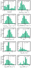 |
Fig. 1. Distributions of observed and physical properties of the LAE sample described in Sect. 2.1. From panel a–j: redshift, Lyα luminosity, Lyα flux, Lyα FWHM, rest-frame Lyα EW, absolute UV magnitude, UV spectral slope, stellar mass, SFR, and sSFR. The Lyα emission shown here has not been corrected by attenuation from dust. The vertical dashed black line indicates the median value, μ1/2 (reported in the top right), of the distributions used to select the subsamples of Sect. 3.2. The vertical dotted gray lines indicate the median absolute deviation. |
The information on the absolute UV magnitude at 1500 Å, MUV, and the UV spectral slope β, panels f and g, computed in H17 (see their Sect. 3.1) is available only for 178 objects in common with their sample. Using the same method as H17, we computed MUV and β for other 26 objects that had at least two HST detections above 2σ in the HST passband filters listed in Table 2 of H17. We caution the reader, however, that the determination of the β slope can be subject to high uncertainties, in particular for weaker sources, with errors as large as one (see Table 3 of H17).
The stellar mass, SFR, and specific SFR (sSFR; panels h, i, and j, respectively) were inferred via SED fitting using the high-z extension of the code MAGPHYS (da Cunha et al. 2008, 2015) and enabling for a minimum stellar mass of 106 M⊙ (see Sect. 3.2 of Maseda et al. 2017). We used HST photometry from the UVUDF catalog of Rafelski et al. (2015) which comprises WFC3/UVIS F225W, F275W, and F336W; ACS/WFC F435W, F606W, F775W, and F850LP and WFC/IR F105W, F125W, F140W, and F160W.
The templates incorporated in MAGPHYS do not include contributions from nebular emission. This does not strongly affect our SED fitting results as the strongest optical emission lines (Hβλ4861, [O III]λ5007 and Hαλ6563) do not fall in any of the HST passband filters used in the fitting process for z > 2.9. However, we note that the weaker [O II]λλ3726,3729 can contaminate the F160W channel for z ≲ 3.2, and Lyα itself falls in the F606W channel for the redshift range of interest in this work. Even if the Lyα EWs are smaller that those of the Balmer lines, this could bias our stellar mass estimates to larger values in some cases (cf., Stark et al. 2013). In addition, the parameters inferred from SED fitting can suffer a certain level of degeneracy as a uniform catalog with deep near-IR (e.g., Spitzer/IRAC) data points, redward of the HST F160W passband filter, is not yet publicly available. For the above reasons, we limited ourselves to using the physical properties, namely stellar mass, SFR, and sSFR, inferred from SED fitting to split the sample in two bins using the median value (dashed lines in all the panels).
Spectroscopic studies in a similar redshift range to the one considered in this work have been performed with VLT/VIMOS and Keck/DEIMOS (Cassata et al. 2011, 2015; Dawson et al. 2007; Pahl et al. 2020). While the limiting magnitude at 1500 Å, MUV of these previous studies is roughly −18, the MUSE HUDF survey has enabled statistical studies of hundreds of fainter LAEs with UV magnitudes in the range of −21.3 < MUV < −15.8. Our observations probe fainter luminosities compared to other samples of LAEs at z ≃ 2 − 3 where the limiting UV magnitude is MUV = −18 (e.g., Erb et al. 2014; Nakajima et al. 2018b) or MUV = −19 in the case of deep VANDELS He II emitters (Saxena et al. 2020), or MUV = −20 for the sample of ∼1000 Lyman-break galaxies from Shapley et al. (2003) (see Fig. 1 of Nakajima et al. 2018b). Previous spectroscopic observations of targets with UV luminosities as faint as those observed in our sample have been mainly performed thanks to gravitational lensing (e.g., Stark et al. 2014; Bina et al. 2016) and for small samples of tens of galaxies.
Our sample does not include LAEs with such high luminosities (LLyα ≳ 1043 erg s−1) as, for example, wider field spectroscopic and narrow band surveys (e.g., Gronwall et al. 2007; Ouchi et al. 2008; Cassata et al. 2011; Sobral et al. 2017; Matthee et al. 2017), which all seem to host an AGN (e.g., Konno et al. 2016; Sobral et al. 2018). We measured Lyα fluxes down to a few ×10−18 erg s−1 cm−2, similar to a few tens of sources from Rauch et al. (2008) and Cassata et al. (2011), while many other surveys probed only the most luminous emitters with Lyα fluxes larger than 10−17 erg s−1 cm−2 (e.g., Ouchi et al. 2008; Sobral et al. 2017). The FWHMs of Lyα are comprised between ≈100 km s−1 and ≈640 km s−1, with a median value of ≈270 km s−1. Our LAEs have a median value of the rest-frame Lyα EW of ≈90 Å and include high Lyα EW values, 34 (9) with EWLyα ≥ 200 (400) Å similar to the extreme emitters detected by Hashimoto et al. (2017b) at z ≈ 2 (see also, Sect. 8.1 of H17 and Maseda et al. 2018). The Lyα EWs of our sample are > 10 Å and on average higher than those found in samples of high-z galaxies selected by photometric redshifts, that is, requiring a detectable continuum in several photometric bands (e.g., Cassata et al. 2015; Cullen et al. 2020). In consequence, many of our galaxies are much fainter in their continua than in other samples, which we exploit in this study.
The UV continuum slope β (fλ ∝ λβ) measured in the rest-frame wavelength interval of ∼ 1700 − 2400 Å (Sect. 3.1 of H17) ranges from ≈ − 3 to 1, with a median value of −1.8. A significant fraction (≈37%) of LAEs have blue UV slopes, β ≲ −2, as those observed in dwarf galaxies at z ≈ 2 (e.g., Stark et al. 2014) and at z ≃ 7 (e.g., Finkelstein et al. 2012; Bouwens et al. 2012, 2013), suggestive of little reddening from dust. The low dust content of most of our LAEs is also supported by the low attenuation in the V-band, AV, inferred from the MAGPHYS fitting tool: median (mean) values of 0.04 (0.11) mag.
This study probes some of the lowest stellar mass objects observed at the redshift range of interest, down to ≈1.6 × 10⁷ M⊙ with SFRs in the range of 0.04 < SFR < 35 M⊙ yr−1. Figure 2 shows the distribution of our MUSE HUDF LAEs in the star formation rate-stellar mass (SFR-M⋆) plane, which overall do not populate areas strongly above the so-called main sequence of galaxies (Noeske et al. 2007; Whitaker et al. 2012) as other z > 2 line emitter galaxies presented in the literature (e.g. Erb et al. 2010; Amorín et al. 2017; Berg et al. 2018). For comparison, we show the distributions of the stellar masses and SFR of 2.4 < z < 5.5 galaxies from the public catalog of the 3D-HST survey (Momcheva et al. 2016), which also include the targets of spectroscopic surveys like VANDELS (McLure et al. 2018). The sSFR, −9.6 < log10(sSFR/yr1) < −7.9, are on average less extreme than those (log10(sSFR/yr−1) ≥ −7.7) found in local and high-z, metal-poor star-forming galaxies and Lyman continuum (LyC) leaker candidates (see Col. 6 of Table 1 from Plat et al. 2019).
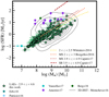 |
Fig. 2. Distribution of the LAE sample (green stars) in the star formation rate-stellar mass (SFR-M⋆) plane. For comparison, values for 2.4 < z < 5.5 galaxies in the 3D-HST survey public catalog by Momcheva et al. (2016) and data for z ≳ 2 star-forming galaxies from Erb et al. (2010), Patrício et al. (2016), Amorín et al. (2017), Vanzella et al. (2017), and Berg et al. (2018) (see also Sect. 5.2) are shown color-coded as labeled in the legend. The curves of the star formation sequence from Whitaker et al. (2014) at 2 < z < 2.5, main sequence (MS) at 2 < z < 3 from Bisigello et al. (2018), and at 3.9 < z < 4.9 from Caputi et al. (2017) and the starburst (SB) sequence at 3.9 < z < 4.9 from Caputi et al. (2017) are shown for reference. |
2.3. Spectral extractions
Three different methods for spatially integrating the data cube and creating one-dimensional spectral extractions are presented in I17 (Sect. 3.1.3): namely the unweighted sum, the white-light weighted, and the PSF-weighted. In this work, we stack PSF-weighted spectral extractions of the 220 LAEs described in Sect. 2.1, as they offer the advantage of a higher S/N of the extracted one-dimensional spectra, a reduced contamination from neighboring objects, and flux conservation that enables easy data comparison. Moreover, the PSF-weighted version is the reference extraction (REF_SPEC in I17) used to compute the spectroscopic redshift for the majority of the sample (215/220). The assignment of a weighted optimal spectra as reference extraction in the MUSE HUDF DR1 catalog depends, as described in Sect. 3.1.3 of I17, on the galaxy size as computed by SExtractor (Bertin & Arnouts 1996) in the HST F775W images from the UVUDF catalog (Rafelski et al. 2015). The PSF-weighted spectrum is adopted for objects with FWHM < 0.7″.
In Sect. 3.2, we group our sample in two bins for each of the properties described in Sect. 2.2, including Lyα properties. As noted in Sect. 3.3 of I17, possible biases on flux measurements introduced by the choice of a weighted extraction could be important, particularly to avoid losing spatially extended line emission, as in the case of the resonant Lyα line. To obtain accurate estimates of the total Lyα emission, we used the Lyα fluxes and EWs recomputed by applying the CoG method (e.g., Sect. 5.3 of Leclercq et al. 2017) accounting for the likely extended emission whose origin is currently a subject of intense discussion (e.g., Wisotzki et al. 2016; Leclercq et al. 2017; Kusakabe et al. 2019). Given that the other UV lines have higher ionization potential, their emission is expected to be less extended than Lyα. We visually inspected the Lyα narrow band images to check against radiation from close companions affecting our Lyα CoG fluxes. We checked that by grouping our sample considering the Lyα properties (flux, luminosity, EWs, and FWHM) computed on the weighted optimal extractions, rather than using the CoG method, the trends described in Sect. 4 and our conclusions (Sect. 6) remain unchanged.
3. Spectral stacking
3.1. Stacking methodology
We statistically combined multiple galaxy spectra to obtain the composite spectrum of different LAE subsamples (defined in Sect. 3.2) and adopted a bootstrapping method to compute the error of the stacked spectra. For most of our sources, the redshift was measured from the Lyα line (see I17), which is often shifted by few hundred km s−1 compared to the systemic redshift (e.g., Hashimoto et al. 2013, 2015; Song et al. 2014; Erb et al. 2014; Trainor et al. 2015; Henry et al. 2015). We therefore computed new redshfits using the empirical correlation between the velocity offset of the Lyα peak and the Lyα FWHM proposed by Verhamme et al. (2018, hereafter V18, Eq. (2)), assuming that the systematic errors are negligible compared to the statistical errors. The uncertainties related to these prescriptions are discussed in Sect. 3.3. We then shifted the spectra of the LAEs to their corrected redshifts and re-binned them to a linear sampling of 0.3 Å (corresponding to the 1.25 Å sampling of MUSE at z ≈ 3). The spectra were averaged over 150 bootstrap iterations in order to compute the noise associated with the stacked spectrum.
There are different possible approaches to combine the spectra from a stack. We used simple unweighted averaging to obtain spectra that are as representative of our LAE subsamples as possible. We decided against the application of any flux-related weighting schemes (e.g., by the inverse variances) because such schemes invariably lead to composites dominated by the few brightest spectra. We compare mean and median stacks, as the brighter and more massive LAEs or galaxies with stronger lines could dominate the signal in the mean spectra of some LAE subsamples. We did consider median stacking in addition to just the mean, which reduces the influence of the brightest and most massive galaxies even further, but at the expense of obtaining a lower S/N in the median composites. Overall, we found that the EWs measured in mean and median stacks are consistent within one standard deviation. The line ratios differ by up to 0.1–0.2 dex comparable with the error measurements of the ratios. The mean and the median stacked spectra of the full sample of LAEs are shown in Fig. 3 (black and blue curves, respectively).
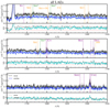 |
Fig. 3. Mean and median spectra of all 220 LAEs described in Sect. 2.1 shown in black and blue with the error displayed via gray and light-blue shaded areas, respectively. The vertical lines indicate the rest-frame wavelengths of some of the main spectral features: nebular emission lines (purple), ISM absorption (orange), and fine-structure transitions (green). The bottom panels show the S/N per pixel (gray and cyan curves for mean and median spectra, respectively) with the dotted red horizontal line indicating S/N = 3. |
We note that the MUSE spectra have not been corrected for dust attenuation due to the complexity of properly modeling the dust embedded in different emitting sources (stars and gas) and to the poor constraints available at high z (e.g., Chevallard et al. 2013; Schaerer et al. 2015; Reddy et al. 2016; Buat et al. 2018, and references therein). Most of the LAEs in our sample have blue UV slopes, suggesting a low dust content. Moreover, SED fitting to the broad-band photometry indicates a median attenuation of 0.11 mag in the V-band. If we take this as proxy for the continuum and nebular attenuation, we can assume a minimum impact from dust on the observed spectra of our LAEs.
3.2. Stacked spectra of LAEs
For each of the properties described in Sect. 2.2, we divided our sample of LAEs in two subsamples adopting as thresholds the median values of the distributions (black vertical lines in the histograms of Fig. 1). This ensures roughly the same number of LAEs for each subsample. It is worth noting that none of the spectra of the individual 220 LAEs have S/N > 3 detections of C III] or any other UV emission lines apart from Lyα (Sect. 4).
We then computed the stacked spectra of all the subsamples in order to study and compare their average spectral properties. As an example, Fig. 4 shows the stacked spectra of fainter and brighter LAEs with log10(LLyα/(erg s−1)) ≤42.0 and > 42.05 (left and right, respectively). All the average spectra of the other subsamples are shown in Appendix A, and their emission line properties are discussed in Sect. 4.
 |
Fig. 4. Mean spectra of LAEs with log10(LLyα/(erg s−1)) ≤42.0 and > 42.05 (left and right, respectively) are shown in black in the top panels, with the error budget displayed via the gray shaded regions. The median values of log10(LLyα/(erg s−1)) for the two subsamples are 41.86 and 42.35, respectively. The vertical lines indicate the rest-frame wavelengths of some of the main spectral features: nebular emission lines (purple), ISM absorption (orange), and fine-structure transitions (green). The bottom panels show the S/N per pixel (gray curves) with the dotted red horizontal line indicating S/N = 3. |
We note that the limited number of sources in our sample prohibits additional binning, and namely splitting them into three or more subsamples. In particular, for lower luminosity and lower mass LAEs, we did not detect emission lines with S/N > 2.5, even though smooth transitions between the stacked spectra could be visually apparent.
3.3. Velocity offset correction
The redshift of the MUSE HUDF galaxies at z > 3 is often determined solely via the Lyα line, which, due to its resonant nature, is often offset by a few hundred km s−1 compared to the systemic redshift (e.g., Hashimoto et al. 2015). Verhamme et al. (2018) propose two prescriptions to recover the systemic redshift from the observed correlations between the separation of the peaks or the FWHM of the Lyα line and the velocity offset of the red peak ( ) with respect to the systemic redshift. As not all the LAEs of our sample show a double-peaked Lyα line profile, we adopted the latter correlation (Eq. (2) of V18). Other empirical prescriptions to recover the systemic redshift of LAEs have been proposed in the literature, such as the relationships between the velocity offset and the Lyα EW proposed by Adelberger et al. (2003) and Nakajima et al. (2018b). The corrected redshifts computed by adopting these two prescriptions differ at maximum by 10% of the uncertainty associated with the redshift computed with Eq. (2) of V18.
By inspecting our stacked spectra, we find some emission line peaks to be redshifted compared to the rest wavelength of the line (Figs. 4 and in Appendix A). For a given stacked spectra, this shift is not the same for all the emission lines, but it varies from 10 to 50 km s−1, reaching values up to 100 km s−1 only when the line has S/N < 2.5. This may suggest that a unique relation is not optimal for all the sources. We consider the subsample split in Lyα FWHM (Fig. A.3) and measure the velocity shift of the peak using the rest wavelengths of the C III] and O III] collisionally excited lines as reference wavelengths. In this way, we obtain, for each line, two points to anchor the relation between the Lyα FWHM and shift of the peak for our LAEs (Fig. 5, green and orange lines). We also consider the mean shift with respect to the two ISM emission features (purple line), which is fully consistent with the V18 relation (in gray). Moreover, the relation obtained using O III] as reference line has a slope very similar to the relation found by Muzahid et al. (2020) obtained from stacking circumgalactic medium (CGM) absorption profiles. It is remarkable how different methods, either object-by-object-based, or averaged over a larger number of sources, provide similar correlations, all within the scatter of the V18 relation.
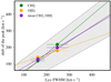 |
Fig. 5. Correlations between shift of Lyα peak and Lyα FWHM obtained from Lyα FWHM subsamples of our LAEs. These correlations were obtained considering the rest wavelengths of C III] (green line) and O III] (orange line) as reference wavelengths and their mean shift (purple line). In gray, Eq. (2) of V18, obtained from object-by-object measurements, and the associated scatter (gray shaded area). |
Given the uncertainty in the systemic redshift of our LAEs, the EWs of the stack are always underestimated compared to true values that one would measure if the correct systemic redshift were known. To investigate to what extent the uncertainty related to the V18 correction affects the spectral measurements of the emission lines presented in Sect. 4.1, we computed two simulated, idealized spectra with constant continuum and FWHMs of 150 and 300 km s−1, respectively. We created 150 copies of these spectra using the same sampling of 0.3 Å as for the LAEs and added random Gaussian noise to each pixel, emulating the continuum S/N of our stack (S/N = 5). We then randomly shifted the line center according to Eq. (2) of V18 (assuming a value for Lyα FWHM of 300 km s−1, close to the median value of our sample) and stacked these idealized spectra with the same method adopted for our real sample of LAEs (Sect. 3.1). We find that EWs of these stacks can be underestimated between 15 and 20% compared to the values of the idealized case. This means that the line EWs measured on the spectra of our LAEs and reported in Table 1 can be up to ≈20% higher than the tabulated value.
Details of the MUSE HUDF LAE subsamples and emission-line EWs measured from the stacked spectra.
4. Results
The mean and median stacked spectra of all the LAEs (Fig. 3) show features in emission and absorption. These include nebular emission lines, like O III] and C III], and absorption features, such as O Iλ1302 +Si IIλ1304 and Si IIλ1527 (hereafter O I + Si II and Si II, respectively). The latter have been identified as uncontaminated tracers of interstellar absorption in the UV spectra of star-forming galaxies (Vidal-García et al. 2017). The other interstellar absorption features that are clearly visible in Fig. 3, Si IIλ1260 and C IIλ1335 (hereafter C II), can be contaminated by nebular emission (Vidal-García et al. 2017). The Si IVλ1403 (hereafter Si IV) ISM absorption feature, which, along with C IV, traces the highly ionized ISM, is also contaminated by stellar wind features. The He II and C IV emission lines are blends of stellar photospheric absorption/winds and nebular emission. In addition, C IV is a resonant line affected by absorption from gas in the ISM and CGM surrounding galaxies. Most of these features have been observed in the stacked spectra of z > 2 galaxies. Interestingly, while the stacked spectra of Shapley et al. (2003) and Saxena et al. (2020) show C IV absorption or P-Cygni, the mean C IV doublet of our LAEs (Fig. 3) is in emission.
This work focuses on measuring the UV nebular emission lines in the mean spectra of the different LAE subsamples (Sect. 4.1) and studying how these features vary with the observational and physical properties of these LAEs (Sect. 5). The stacked spectra of the LAE subsamples show a large variety of nebular emission lines, absorption features, and fine structure transitions, as shown in Figs. 3 and 4, and in Appendix A. None of the 220 LAEs have UV emission lines other than Lyα detected in their individual spectra with S/N > 3. The only exception is ID3621, in the mosaic field, for which the He II line is detected with S/N > 2.5 (Nanayakkara et al. 2019).
In the stacks of Figs. 4 and Appendix A, we identify some of the main UV nebular emission lines that are currently detected in the spectra of high-z or local, metal-poor star-forming galaxies (e.g., Erb et al. 2010; Stark et al. 2014; Berg et al. 2016, 2018, 2019; Patrício et al. 2016; Vanzella et al. 2016, 2017; Nakajima et al. 2018b). Namely, we detected the collisionally excited O III] and C III] doublets, and, in few cases, Si III], as well as the He II emission feature. In addition, we observed different profiles of the C IV resonant doublet, as discussed in Sect. 4.2. Depending on the observed and physical properties of the LAEs, the stacked spectra of several subsamples exhibit absorption features and fine-structure transitions (see Sect. 5). A quantitative study of these features would require a complex modeling that combines stellar continuum, nebular emission and resonant scattering through the ISM and CGM. This is beyond the scope of the current analysis and will be the subject of future works.
4.1. O III], C III], Si III], and He II lines
We computed EWs of He II, O III], C III], and Si III] by performing a Gaussian fit to the portion of the spectrum that contains the emission line, fixed to the systemic redshift; in particular, we fit the line doublets as a sum of two Gaussian functions. The continuum is defined by calculating the mean flux within a window of 100 Å around the emission lines, excluding the central 10 Å around the rest wavelengths of the line features. We note that we did not subtract the stellar continuum during this fitting procedure. This should not strongly affect the collisional lines such as C III] and O III], but multiple mechanisms are known to contribute to the recombination He II line, which has both a nebular and stellar origin. For this reason, the width of the He II line is free to vary in the fit. We found its FWHM to be from 0.6 to 2.5 times that of C III] and O III], consistent with the results from Nanayakkara et al. (2019, Fig. 16). In our case, the possibility of constraining the potential contribution from Wolf-Rayet stellar winds to the total He II flux is hampered by the low S/N. Given the current limitations of theoretical models in correctly reproducing the nebular He II and the uncertainties in modeling the continuum emission from massive stars (e.g., Senchyna et al. 2017; Berg et al. 2018; Nanayakkara et al. 2019; Plat et al. 2019), here we simply provide the integrated fluxes obtained from the Gaussian fitting, without including additional uncertainties in the decomposition of the different mechanisms that can power the He II feature.
The values of the EW of lines detected with S/N > 2.5 in the composite spectra of the different subsamples (and of the complete 220 LAEs sample) are reported in Table 1. In some cases, and in particular for the faintest subsamples, even if the emission features are clearly visible in the stacked spectra, the noise prevents S/N > 2.5 line detections. The EW values of the lines with S/N < 2.5 are reported as 1-σ upper limits in Table 1. No value is reported in the event of non-detection, meaning when the line is embedded within a highly noisy continuum level. The nebular-line EWs for the different LAE properties are shown in Fig. 6, while a comparison with other measurements from the literature and line ratios are shown in Figs. 8 and 9 (Sect. 5.2).
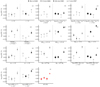 |
Fig. 6. EWs of He II, O III]λ1666, [Si III]λ1883, and [C III]λ1907 for the different subsamples of MUSE HUDF LAEs (x-axis). The symbols refer to different emission lines, as labeled in the legend. Smaller and larger symbol sizes indicate the subsample of LAEs whose properties are lower and higher than the median value, respectively. Empty symbols with downward arrows indicate upper limits, while non-detections are shown by the black dash. Red symbols show the EWs for all 220 LAEs in the sample. |
The [C III]λ1907 blue component of the C III] doublet is detected in almost all the stacks except for z > 3.6. Out of the five stacked spectra where both components are detected, four show a [C III]λ1907 / C III]λ1909 ratio in excess of the value expected in the low-density limit (1.53), implying electron densities ≳103 cm−3 (see Sect. 4.1 of Maseda et al. 2017). We detected the O III]λ1666 component of the O III] intercombination doublet in all the stacks except for the log10(LLyα/(erg s−1)) ≤ 42.05, log10(FLyα/(erg s−1 cm−2)) ≤ −17.02, LyαFWHM > 271 km s−1, Lyα EW ≤97.2 Å and β > −1.79, while the typically weaker blue component of the doublet is never detected with S/N > 2.5. The He II line is observed in the stacks of LAEs with more intense Lyα emission, MUV ≤ −17.9, bluer UV slope, and a higher stellar mass and SFR. The Si III] doublet is detected with S/N > 2.5 only in the stack of the total sample, but not in those of the subsample split. In Col. 6 of Table 1, we report 1σ upper limits for the [Si III]λ1883 component, as this is stronger than Si III]λ1892 for electron densities < 105 cm−3.
4.2. CIV doublet and absorption features
Figure 7 shows the C IV resonant doublet, the Si II interstellar absorption, and the SiII*λ1533 (hereafter SiII*) fine-structure transition for the composite spectra of the LAE subsamples. Multiple physical processes can contribute to the observed C IV spectral profile, like stellar winds in massive O and B stars, nebular emission and absorption in the ISM and CGM (e.g., Vidal-García et al. 2017; Byler et al. 2018; Berg et al. 2018). Producing C IV emission requires photons with energies (> 47.9 eV) associated with hard ionizing radiation fields from massive stars, AGN, and radiative shocks. The C IV doublet is currently receiving a great deal of attention, as it is one of the strongest UV lines measured at high z (e.g., Stark et al. 2015a; Mainali et al. 2017; Schmidt et al. 2017; Vanzella et al. 2017; Berg et al. 2018) and in local metal-poor galaxies (e.g., Senchyna et al. 2017, 2019; Berg et al. 2019). Disentangling the multiple physical mechanisms contributing to the C IV profile requires a proper modeling of the stellar continuum, as well as of the resonant scattering through the medium within and around galaxies. A self-consistent modeling of photon scattering is important for the interpretation of the shapes of the interstellar absorption features, for example, Si II, and will be the subject of another work (Mauerhofer et al., in prep.). In this work, we limit ourselves to a qualitative discussion of the appearance of the C IV feature and of the main absorption features.
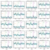 |
Fig. 7. Zoom-in around the rest wavelengths of the C IVλλ1548,1551 doublet (purple vertical lines) for the different averaged spectra (black lines) of the MUSE HUDF LAEs (as described in the title of each panel). The light blue shading indicates the noise. The other vertical lines indicate the rest-frame wavelengths of the Si IIλ1527 ISM absorption feature (orange) and the SiII*λ1533 fine-structure transition (green). |
We observed C IV with a P-Cygni profile in the stacked spectra of LAEs with higher Lyα luminosity and flux, lower Lyα EW, brighter UV magnitudes, redder UV slopes, higher masses, and higher SFRs (Fig. 7). The origin of this P-Cygni profile can be associated with the presence of stellar winds from OB stars and depends both on the stellar metallicity and the relative fractions of O and B stars. Instead, the average spectra of LAEs with lower Lyα FWHM, higher Lyα EW, fainter UV magnitude, bluer UV slope, lower stellar mass, and lower SFRs show an emission-line doublet at the C IV rest wavelengths, with no sign of absorption on the blue side. In these cases, the nebular emission from ionized gas dominates the spectra. This is indicative of very low (Z < 0.002) interstellar metallicity (see for example Figs. 15 and 18 of Vidal-García et al. 2017). We fit two Gaussian profiles to the C IV emission doublet, meaning under the assumption that nebular emission dominates the feature profile in the stacked spectra, without evidence of a P-Cygni profile, and we found C IV EWs ranging between 1.95 and 4.74 Å.
The Si IV interstellar absorption exhibits a behavior similar to that of C IV and appears in absorption or P−Cygni when C IV is in P−Cygni, while it is reduced, if not suppressed, when the C IV nebular emission dominates the profile. Absorption in the ISM or CGM can also play a significant role in shaping the C IV profile. In addition, stellar Si IV P−Cygni, which is a signature of stellar winds, can be contaminated by interstellar lines of the same element. Interestingly, the appearance of low-ionization absorption features resemble those of C IV and Si IV. In particular, C II and Si II are in absorption when C IV shows a P-Cygni profile, as in the cases of higher Lyα FWHM, lower Lyα EW, redder UV slope, and more massive LAEs. This is suggestive of common variables, likely stellar mass and SFR, driving the spectral differences between the LAE subsamples, as discussed at the end of Sect. 5.1.
5. Discussion
5.1. Dependence of UV line features on galaxy properties
The main goal of this paper is to investigate how the UV spectral features of continuum faint (−20 ≲ MUV ≲ −16 ) and low-mass (107 ≲ M⋆ ≲ 1010 M⊙ ) LAEs at 2.9 ≤ z ≤ 4.6 vary with their properties. These variations can be appreciated in Figs. 6 and 7 and are discussed below.
5.1.1. Redshift
The stacked spectra of LAEs in the two redshift intervals (Fig. A.1) do not show strong qualitative differences in the absorption and emission features. A more quantitative comparison is hampered by the low S/N at z > 3.6. For example, the non-detections of [Si III]λ1883 and the upper limits of C III] in the higher redshift subsample are hardly ascribable to a difference in terms of physical properties, but can be associated with a higher spectral noise of z > 3.6 LAEs. This is because of the higher luminosity distance and the higher noise level due to the sky emission at a longer wavelength. However, the limits derived from the higher z subsample are still consistent with those of the lower z stacked spectra (panel a of Fig. 6).
5.1.2. Lyα luminosity and flux
Even though most of the emission lines are clearly visible in the mean spectra of LAEs in different bins of Lyα luminosity and flux, the He II, O III]λ1666 and C III]λ1909 lines are detected with S/N > 2.5 only in the composite spectra of the brightest (log10(LLyα/(erg s−1)) > 42.05 and log10(FLyα/(ergs−1cm−2)) > −17.02) LAEs (panels b and c of Fig. 6). This is mainly due to the, on average, higher continuum S/N of a single spectrum for the brightest sources, as most of them have stronger Lyα emission. This is also the case for the stacked spectra of the higher SFR bin, reflecting that, to first order, the Lyα luminosity scales with the SFR (e.g., Sobral & Matthee 2019). The spectral stacks of the brightest LAEs (Figs. 4 and A.2) exhibit typical absorption profiles of stellar winds, such as C IV and Si IV. Theoretical models predict the strengths of these features to be higher at younger ages and increase from low to high stellar metallicities (e.g., Vidal-García et al. 2017; Byler et al. 2018). Given the absorption features (Si II, O I + Si II, C II) in the spectra of brighter Lyα subsamples, one cannot neglect a contribution from gas and dust in the ISM and CGM in shaping the P−Cygni profiles. If this is the case, the differences between the Lyα-faint and -bright subsamples (Fig. 7) can be explained in terms of photon scattering through a larger amount of gas and dust in the ISM of the brightest sources, which are, in general, more massive. This scenario is strengthened by the stacked spectra for LAEs grouped in mass, where the more massive LAEs show stronger P−Cygni profiles and absorption features. An alternative or additional explanation is that C IV photons are scattered out by outflowing gas in the CGM escaping at larger radii. The stacked spectrum of less luminous LAEs show C IV nebular emission (Fig. 7), with no evidence of absorption, which is indicative of low metallicities. However, the low S/N of the stacked spectra of UV fainter sources reduces our ability to clean the nebular emission of contamination from stellar and interstellar absorption. In a recent work on z ∼ 5 star-forming galaxies, Pahl et al. (2020) concluded that the increase of Lyα strength and the detection of strong nebular C IV emission points toward elevated ionized photon production efficiency. In the case of our sample, this is further supported by detection of the He II recombination line (which requires photons with energy > 54 eV) in the stacked spectra of our brightest LAEs.
5.1.3. Lyα FWHM and EW
The EWs of the [C III]λ1907 and O III]λ1666 collisionally excited emission lines are more than 0.2 dex larger in the mean spectra of LAEs with FWHM ≤271 km s−1 and with Lyα EW > 97.2 Å (panels d and e of Fig. 6). An increase of C III] with increasing Lyα EW has been observed in previous works (e.g., Shapley et al. 2003; Stark et al. 2014; Nakajima et al. 2018b; Du et al. 2018). This is interpreted as a common mechanism dominating the emission of collisionally excited UV lines and the production and escape of Lyα radiation. A higher ionizing photon production by young and metal-poor stars for stronger Lyα EWs reduces the neutral covering fraction and allows more photons to escape the galaxy (e.g., Du et al. 2018). This would be consistent with the scenario in which the extended Lyα radiation (more than 50% of the total Lyα radiation in a galaxy comes from extended haloes, e.g., Leclercq et al. 2017), or a fraction of it, is radiation produced in star-forming regions scattered in an outflowing medium. However, while the relation between Lyα and C III] EWs seems to hold for LAEs with similarly high Lyα EW to those considered in this work, it becomes weaker when galaxies with lower Lyα EW or Lyα in absorption are considered. For example, Le Fèvre et al. (2019, Fig. 6) found a broad scatter between the EW of Lyα and that of C III], and also a fraction of galaxies with significant C III] emission and Lyα in absorption.
For LAEs with higher FWHM or smaller EW, the [C III]λ1907 and O III]λ1666 EWs are smaller because of the stronger underlying continuum as result of a more intense star formation. The mean SFR is 0.3 and 1.2 M⊙ yr−1 for lower and higher FWHM subsamples splits, respectively. Similarly, the LAEs have a mean SFR of 0.4 and 1.35 M⊙ yr−1 for the larger and smaller EW subsamples.
C IV is in emission for the LAEs with lower FWHMs, while in the case of higher FWHMs, the C IV P-Cygni profile and interstellar absorption features are clearly visible (Fig. 7). The C IV doublet is observed in emission (C IV EW of 4.2 Å) for large Lyα EW, while the C IV profile is unclear for the stacked spectra of the subsample with smaller Lyα EW. If we neglect the stellar continuum, these differences in the Lyα and C IV profiles between the subsamples with lower/higher FWHMs and larger/smaller EWs can be interpreted as radiation transfer through a different amount of gas. The emission from resonant lines can be similarly affected if they are seen through the same gas, as is also shown for the Lyα and Mg IIλ2800 doublet in local “green pea” galaxies (e.g., Henry et al. 2018). However, Lyα and C IV trace different phases of the medium within and around galaxies. While Lyα profiles are shaped by resonant scattering in the neutral gas, C IV traces the highly ionized gas. Our result would suggest that a lower amount of neutral gas implies a lower amount of ionized gas. A Spearman’s correlation coefficient of 0.52 supports a moderate dependence of Lyα FWHM with stellar mass. Similarly, smaller EW LAEs (which would correspond to a lower amount of gas) have higher stellar masses. This is consistent with the mean spectra of LAEs with higher stellar mass exhibiting C IV in P-Cygni profile. A higher fraction of neutral gas for higher Lyα FWHM and lower Lyα EWs is also supported by the presence of stronger low-ionization absorption features in the stacked spectra of these subsamples. A correlation between low-ionization absorption lines and Lyα EW, stellar mass, UV luminosity, and β slope has been observed in LBG at z ≈ 3 by Jones et al. (2012) and explained in terms of star formation-driven outflows of neutral gas responsible for Lyα scattering and the strong low-ionization absorption lines, while increasing stellar mass, metallicity, and dust content. Our results are consistent with their picture, as low-ionization absorption features are stronger for redder UV slopes (higher dust content), larger stellar mass, higher SFR, and brighter LAEs.
5.1.4. UV magnitude and spectral slope
The stacked spectra of the UV fainter LAEs exhibits larger (> 0.5 dex) O III]λ1666 and [C III]λ1907 EWs than the UV brighter subsample (panel f of Fig. 6). Very interestingly, a clear C IV in emission (C IV EW of 3.9 Å) is observed in the mean spectra of the fainter (MUV > −17.9) LAEs (Fig. 7), indicative of a hard ionization field, such as that from young and massive stars, and of an elevated ionized photon production efficiency. The UV spectral slope is considered a proxy for the dust content as well as for the hardness of the ionizing radiation. Since the fainter sources have, on average, bluer colors (Fig. 2 of H17), the subsample splits in β present similar stacked spectra to those of the MUV subsamples (Figs. A.5 and A.6). With the cautiousness on the uncertainties related to the β slope calculation (Sect. 2.2) in mind, we note that LAEs with bluer UV slopes show C IV in emission (C IV EW of 1.95 Å). They also have C III] EWs more than 0.2 dex larger than LAEs with higher β. In the case of LAEs with redder slopes, deep absorption features suggest the presence of a higher fraction of neutral gas in the ISM and CGM of these sources. The harder ionization field of the bluer LAEs is confirmed by the detection of the He II line in emission. The UV fainter LAEs of our sample have, on average, higher Lyα emission strengths (LAEs with MUV> and ≤ − 17.9 have average Lyα EWs of 201 and 76 Å, respectively), which implies higher ionzing photon production rate in stronger LAEs. These results are in line with current detections of C IV and He II in emission in low-mass, UV-faint star-forming systems in the local Universe (e.g., Senchyna et al. 2017; Berg et al. 2019) and at z ≈ 2 − 3 (e.g., Berg et al. 2018; Nakajima et al. 2018b).
5.1.5. Stellar mass, SFR, and sSFR
The stacked spectrum for the lower stellar mass bin shows, in addition to the C IV doublet in emission, [C III]λ1907 and O III]λ1666 EWs are 0.3 dex larger compared to that of the higher mass bin (panel h of Fig. 6). At the same time, the stacked spectra of the higher mass LAEs show absorption features that are not clearly observed in the spectra of the lower mass subsample (Fig. A.7). The [C III]λ1907 and O III]λ1666 EWs are stronger (0.6 and 0.4 dex, respectively, panel i of Fig. 6) for the lower SFR subsample as LAEs with low SFR are, on average, less massive. High SFR implies a strong emission continuum. As already mentioned, the C IV doublet varies from emission to P-Cygni with increasing stellar mass and SFR. A similar behavior has been observed for the also resonant Mg II doublet (e.g., Finley et al. 2017; Feltre et al. 2018).
The mean spectra of LAEs with higher sSFR have larger C III] EW. This has been found to correlate with the EW of the optical [O III]λ5007 line (Maseda et al. 2017), which in turn correlates with the sSFR for low-metallicity starbursts (Tang et al. 2019). It is not possible to discuss the trends of the other features as a function of sSFR because of the difficulty in detecting emission features in the stacked spectra of LAEs with higher sSFR, as these are also among those with the lowest UV luminosity, and therefore have individual spectra of lower S/N.
The similarity of the variation of spectral features among the LAE subsamples implies that these spectral differences contain important information on the physics of galaxies and that these are mainly dictated by SFR and stellar mass, which are intrinsically linked to differences in ages, metallicity and dust content of galaxies.
5.2. Comparison with the literature
With caution for uncertainties on the systemic redshift in mind (Sect. 3.3), we investigated how the line measurements described in Sect. 4.1 compare with those already presented in the literature. We considered data from local metal-poor galaxies (Fig. 8) and strong line emitters at z ≥ 2 − 3 (Fig. 9), which are both considered valuable examples of the young galaxies that could have significantly contributed to the ionizing photon budget necessary to sustain cosmic reionization. Figures 8 and 9 show comparisons of EWs and line ratios of the MUSE HUDF LAEs with those from the literature. The spectra of our LAEs have not been corrected for potential attenuation by dust in order to avoid using an arbitrary attenuation curve, while the data from the literature have been corrected as described in the corresponding works. The impact of this on our analysis is negligible, as we considered the C III]/He II, C III]/O III]λ1666, O III]λ1666/He II line ratios that would differ by ≈0.1 dex assuming a V-band attenuation of one order of magnitude (AV = 1) and the Calzetti et al. (2000) curve (see also, Sect. 5.1 of Hirschmann et al. 2019). By adopting an AV = 1 mag, we would vastly overestimate the dust content of our LAEs. As discussed in Sect. 3.1, the SED fitting to the HST photometry indicates a mean attenuation of 0.1 mag in the V-band, and the blue UV slopes of our LAEs are in line with a low dust content.
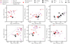 |
Fig. 8. UV emission line properties of MUSE HUDF LAE subsamples and local galaxies from the literature described in Sects. 4.1 and 5.2. The diagrams show different combinations of EWs and ratios of the He II, O III]λ1666, C III], and [C III]λ1907 emission lines. Different black symbols refer to S/N > 2.5 line detections for different LAE subsamples and the red cross to the total LAE sample. Smaller and larger symbols indicate the subsample of LAEs whose property is lower or higher than the median value, respectively. Different colors refer to different samples from the literature, as labelled in the legend. Open and filled symbols indicate upper limits and detections, respectively. The left triangles refer to local galaxies. The gray dashed lines are the separation criteria between AGN and star-forming galaxies from Nakajima et al. (2018b), while the gray dotted lines represent the selection criteria for the AGN, composite, and star-forming galaxies from Hirschmann et al. (2019). |
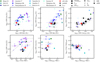 |
Fig. 9. Same as Fig. 9. Open and filled symbols indicate upper limits and detections, respectively. The pentagons refer to data for 2 ≤ z ≤ 4 galaxies. |
Comparison with local metal-poor galaxies. Figure 8 shows measurements performed on local low-mass, metal-poor (Z ≲ 10 − 20% Z⊙) star-forming systems with sSFRs from 1 up to ∼102 Gyr−1 (Berg et al. 2016, 2019; Senchyna et al. 2017, 2019) and 0.13 < z < 0.3 green pea galaxies from Ravindranath et al. (2020). In particular, Senchyna et al. (2017) observed a marked transition in the spectral properties of the UV features with decreasing metallicity. Their star-forming systems with Z < 1/5 Z⊙ showed more prominent nebular emission in He II and C IV, and weak, if not absent, stellar wind features compared to the less metal-poor targets in their sample. Our LAE subsamples show similar spectral variations. For example, the prominent nebular emission lines (C IV, O III], C III]) observed in lower mass, UV faint but higher Lyα EW LAEs require a strong ionizing radiation field and unveil the role of young and metal-poor massive stars in dominating the spectra of these sources. This reveals a strong interplay between the physical properties, such as stellar mass and SFR, and therefore age and metallicity, in driving the differences in spectral features.
The O III]λ1661 and [C III]λ1907 EWs of the mean spectra of our LAEs are, on average, lower (0.3 and 0.5 dex, respectively) than those in the local systems (Fig. 8) and compatible only with the upper limits from Senchyna et al. (2017, 2019). Our LAEs have emission line EWs similar to those of the local metal-poor galaxies for the bluer, lower stellar mass and higher Lyα EW subsamples. These are the properties that characterized the local galaxies considered for this comparison. The C III] EWs of the 0.13 < z < 0.3 green pea galaxies from Ravindranath et al. (2020, Table 3) are < 10 Å and reach values as low as the lowest of our LAEs, in addition to 1-σ upper limits with C III] EW < 1 Å, indicating even weaker emission for the green pea galaxy sample.
The ratios of the collisionally excited O III]λ1666 and C III] lines to the He II recombination line is about 0.2 dex lower in our LAEs than the ratios measured in the local Universe, suggesting a more intense ionizing radiation field for our LAEs, which would increase the He II emission. This is also supported by the stronger EWs of the C IV nebular emission measured on our stacks compared to those of the local sources. An increase from low to high z in the ionization parameter (i.e., the ratio of the number of H-ionizing photons to the number of atoms of neutral hydrogen), which is linked to SFR, or in the ionizing photons’ production efficiency can explain this small difference in line ratios. In addition, the differences in the spectral properties of local sources are affected by the target selection, given that the low-z galaxies considered here have been selected to be extremely metal-poor galaxies with bright optical emission lines.
Comparison with z ≈ 2−4galaxies. High-ionization UV lines have been detected in the spectra of z ≳ 2 galaxies through gravitational lensing (e.g., Stark et al. 2014; Patrício et al. 2016; Vanzella et al. 2016, 2017; Berg et al. 2018), spectral stacking (e.g., Nakajima et al. 2018b; Rigby et al. 2018; Saxena et al. 2020), and deep spectroscopic observations (e.g., Erb et al. 2010; Maseda et al. 2017; Amorín et al. 2017; Nanayakkara et al. 2019). The EWs of He II, O III]λ1666, and C III] from these works are larger than those measured in the average spectra of our LAEs, with the exception of some of the MUSE sources at z ≳ 3 studied by Patrício et al. (2016) and Nanayakkara et al. (2019), some of the stacks from Nakajima et al. (2018b), and some of the VANDELS He II emitters from Saxena et al. (2020). The EWs from Nakajima et al. (2018b) are computed from average spectra of a z ≈ 3 LAE population whose median UV luminosity is about two orders of magnitude brighter than ours. Most of the 2.4 < z < 3.5 UV-selected, low-luminosity galaxies from Amorín et al. (2017) have higher He II and C III] EWs, most likely because of their higher SFR (see Fig. 2). The line measurements from Saxena et al. (2020) are performed on the stacked spectra of UV continuum, bright He II emitters (−19 < MUV < −22). The strong line emitters from Erb et al. (2010) and Berg et al. (2018) are brighter and more massive than the median value of our LAEs. The lensed galaxies from Vanzella et al. (2016, 2017) are among the least massive, most metal-poor, young, and faintest systems observed at z ∼ 3. With MUV > −16, the source ID14 from Vanzella et al. (2017) is roughly one order of magnitude fainter that the faintest LAE in our sample, while the source ID11 from Vanzella et al. (2016) has an remarkable blue UV slope (β = −2.95). Recently, Du et al. (2020) measured C III] EWs in z ∼ 2 analogs of galaxies in the reionization era, obtaining values from 13.2 Å down to 1 Å, reaching values as low as those of our LAEs. The authors also found differences in the C III] EW depending on the selection criteria, with higher values of C III] EW for emission lines rather than for continuum-selected galaxies. Mainali et al. (2020) detected two targets with C III] emission reaching EW ≈ 17 − 21 Å in the spectra of z ∼ 2 galaxies selected for their strong rest-optical line ([O III]λ5007+Hβ) EWs. These values are above the ones of our LAEs and are similar to those observed at z > 6 (e.g., Stark et al. 2015b, 2017; Hutchison et al. 2019).
Interestingly, the line ratios (bottom panels of Fig. 9) of z ≈ 2 − 4 galaxies from the literature are consistent with those measured for our LAEs, suggesting comparable ISM conditions at these similar redshift ranges. The fact that the targets from the aforementioned published works have been selected as strong line emitters can explain the difference in terms of EW strengths. Our results indicate that these extreme emitters may not be representative of the whole population of UV-faint, low-mass LAEs at z ≳ 3.
Comparison with z ≳ 6 galaxies. In recent years, the detection of high-ionization nebular emission lines, such as C IV, C III], and He II, has been possible in the deep rest-frame UV spectra of z ≳ 6 rare, very bright, or gravitationally lensed galaxies (e.g., Sobral et al. 2015, 2019; Stark et al. 2015b,a; Mainali et al. 2017; Schmidt et al. 2017; Mainali et al. 2018; Hutchison et al. 2019). In particular, the C IV EWs measured from the spectra of high-z galaxies with UV magnitude in the same range as our LAEs (MUV ≥ −21) are larger than 20 Å (see Fig. 6 of Mainali et al. 2018). These extreme values are compatible with those measured in obscured AGN but also with photo-ionization by young and massive stars (Stark et al. 2015a). These values are, however, at least four times higher than the C IV EWs of the average of our LAE subsamples showing the C IV doublet in emission. This could reflect a harder ionizing radiation field associated with young, hot, and metal-poor stars, as well as a much higher ionizing photon production efficiency at high redshift (Sect. 4.4 of Nanayakkara et al. 2020). We also have not yet detected a less extreme population of z ≳ 6 faint and low mass galaxies exhibiting spectral properties similar to the average ones of faint LAEs at 3 ≤ z ≤ 4.6, probably because of the selection methods (e.g., Du et al. 2020). Spectroscopic studies of galaxies in the first billion years (z ≳ 6) are still confined mainly to a few gravitationally lensed or exceptionally bright sources with spectral information limited to a few emission lines, along with upper limits, per target, preventing any statistical comparison with lower z sources.
5.3. AGN and other ionizing sources
It is worth investigating the possible contributions from AGN to the average spectra of the MUSE HUDF LAEs. We can exclude the possibility that the mean spectra of our LAEs are dominated by AGN for several reasons. First, our LAEs do not have Lyα FWHMs larger than 1000 km s−1, which would indicate a broad-line AGN (see e.g., Sobral et al. 2017). Second, the LAE subsample with the larger FWHM does not show the C IV doublet, which can be used as proxy for AGN activity (e.g., Mignoli et al. 2019), and we do not detect N V emission, which requires photons with energy > 77.4 eV and is usually a tracer of the presence of an AGN (e.g., Laporte et al. 2017; Sobral et al. 2018). In addition, we discarded the objects defined as X-ray AGN in the 7 Ms Source Catalogs of the Chandra Deep Field-South Survey (Luo et al. 2017, see Sect. 4.5 for source classification) from our sample. Even the deepest X-ray stacks yielded no signal for high-z LAEs (Urrutia et al. 2019; Calhau et al. 2020).
Moreover, by exploring diagnostic diagrams based on EWs and ratios of other rest-UV emission lines (C IV, He II, O III], C III], e.g., Feltre et al. 2016; Nakajima et al. 2018a; Hirschmann et al. 2019), we note that the C III]/He II and O III]λ1666/He II ratios of our LAEs are > 1 and 0.3, respectively, and thus not compatible with pure AGN photo-ionization models (Fig. A1 of Feltre et al. 2016). The low values of C III] and C IV EW (≤ 20 Å) exclude a dominant AGN contribution to the spectral emission (Nakajima et al. 2018a; Plat et al. 2019). Our LAEs would instead be classified as composite (AGN and star-forming) galaxies in the diagrams from Hirschmann et al. (2019) whose selection criteria are, however, customized for massive galaxies (≳109.5 M⊙). We caution that current photo-ionization models for star-forming regions can underestimate, even by one order of magnitude, the He II nebular emission of local metal-poorlocal met (below 1/5 solar), dwarf, and z ≳ 2 galaxies (e.g., Jaskot & Ravindranath 2016; Steidel et al. 2016; Senchyna et al. 2017; Berg et al. 2018), including those detected in our stacks, and MUSE individual spectra (e.g., Nanayakkara et al. 2019). In this context, the reliability of the UV selection criteria for AGN for our LAEs may be reduced, and further improvements in the modeling of the He II ionizing flux from young and metal-poor stellar populations (single stars or binaries) could bring the predictions for nebular emission from star-forming galaxies into agreement with the spectral properties measured in our LAEs.
The presence of strong He II emission implies the need for a hard ionizing spectrum (see e.g., Fig. 1 of Feltre et al. 2016) able to provide photons with sufficient energy to doubly ionize helium (54 eV) that, subsequently, recombines giving rise to He II emission. At the moment, in addition to refinements to the models of young and metal-poor stars, an additional source of harder ionizing radiation seems to be the most likely explanation to account for the measured He II flux. This includes weak AGN or a contribution from other sources, such as exotic Pop III stars, X-ray binaries, radiative shocks, and super-soft X-ray sources such as accreting white dwarfs (Shirazi & Brinchmann 2012; Kehrig et al. 2015; Woods & Gilfanov 2016; Schaerer et al. 2019; Plat et al. 2019).
6. Summary and conclusions
The MUSE HUDF enabled spectroscopic observations of faint (−20 ≲ MUV ≲ −16) and low-mass (between 107 and 1010 M⊙) LAEs at z ≳ 3. Information about the gas emission in these systems comes mainly through the Lyα line which is the strongest emission line in UV spectra. We selected a sample of 220 LAEs and performed spectral stacking to explore the UV emission and absorption features that are too weak to be detected in single spectra. Stacked spectra were computed for different subsamples, partitioned on the basis of both observed (Lyα luminosity, flux, FWHM and EW, UV magnitude, and UV slope) and physical (stellar mass, SFR, and sSFR) properties of the LAEs.
The main focus of this work was to investigate spectral differences of the ionized gas emission features for LAEs with different properties. We were able to detect emission lines such as He II, O III], Si III], and C III], as well as the C IV doublet. The main results of this analysis are summarized below.
-
With the obvious exception of Lyα, the individual deep MUSE spectra do not show the presence of other UV lines, which are clearly detected in the spectra of galaxies. That they appear in the stacked spectra suggests weak UV emission is ubiquitous in the general population of faint and low-mass LAEs, regardless of the differences among the LAE stacks (Sects. 4.1 and 4.2).
-
The C III] and O III] collisional excitation doublets vary with the observed properties in which LAEs have been subsampled (Sect. 5.1). In particular, we find that the C III] EW of our 2.9 ≤ z ≤ 4.6 LAEs increases with that of Lyα EW, similarly to what observed at z ≈ 2 in faint dwarf galaxies (Stark et al. 2014) and in stacked spectra of z ≈ 3 galaxies that are on average much brighter than our LAEs (Shapley et al. 2003; Nakajima et al. 2018b). We note, however, that the relation between the Lyα and C III] EW can present a larger scatter when extended to LAEs with lower Lyα EWs and Lyα emission in absorption (e.g., Le Fèvre et al. 2019). We find larger C III] and O III] EWs in the spectral stacks of the UV fainter and bluer LAEs.
-
We detect the He II emission feature in the mean spectra of brighter, bluer and intensively star-forming LAEs of our sample (Sect. 4.1). The strengths of He II emission are consistent with those observed in other local and z > 2 galaxies, which are challenging current stellar evolution models (Sect. 5.3).
-
We find two different main profiles for the C IV doublet, namely P-Cygni profiles and emission, without clear signs of blue-shifted absorption. These different C IV profiles encode information on the main mechanisms shaping this feature, such as stellar winds from massive stars, nebular emission from ionized gas, and the presence of a neutral medium and outflowing gas. At the same time, the differences that we observe among the stacked spectra suggest that the shape of the C IV profile could also be used as a proxy for galaxy properties. For example, we observe C IV purely in emission in the stacked spectra of low stellar mass, faint, and blue LAEs at 2.9 ≤ z ≤ 4.6 (Sects. 4.2 and 5.1).
-
The emission features detected in our LAE stacked spectra are overall in agreement with those measured for other MUSE sources at similar redshifts and with metal-poor, low-mass star-forming systems in the local Universe (Sect. 5.2). One exception is the He II and C III] EWs of z ∼ 2 analogs of galaxies in the reionization era, which are higher than the average values of our LAEs, likely because of the emission-line selection criteria and their intense SFR, or both. Moreover, the O III]λ1666/He II and C III]/He II ratios of our LAEs are smaller than those of the local dwarf galaxies. This is likely to be because of a variation in production efficiency, strength, and hardness of the ionizing radiation.
The variations in the emission and absorption features in the different spectra are mainly dictated by SFR and stellar mass, which are intimately related to the stellar ages, metal, and dust content of galaxies. This observational evidence could be coupled with theoretical predictions for galaxy evolution to investigate whether the observed trends of the spectral features enable the identification of a given galaxy’s evolutionary phase in the SFR-M⋆ plane.
The stacked spectra presented in this work can be exploited to understand the properties of stellar populations and ionized-versus-neutral gas in faint, low-mass LAEs at high z. While the presence of carbon and oxygen UV lines (O III], C III], and C IV) provides important constraints on the C/O abundance ratio, the absence of hydrogen lines other than Lyα in the UV regime, whose complex resonant nature seriously hampers any estimate of the intrinsic nebular flux, may challenge the estimates of the oxygen abundance (O/H). The latter can be directly probed through rest-frame optical spectroscopy (e.g., [O III]λ5007 and hydrogen Balmer lines), which, in addition, offers the possibility of exploiting standard strong line diagnostics of the properties of the ionized gas such as metallicity, density and ionization level. Regarding our LAEs, additional information from rest-frame optical lines (e.g., from Keck/MOSFIRE or, in the future, from JWST/NIRSpec) will play a crucial role in determining the physical conditions (SFRs, ionization conditions, and gas-phase metallicities) within them, and further constraining the ionizing photon production rates from stellar population models.
To conclude, our stacked spectra are the only available empirical templates of faint and low-mass LAEs, and they will be instrumental to the design of spectroscopic observations of higher z galaxies, including targets in the epoch of reionization, with future facilities (e.g., JWST, ELT)1.
Acknowledgments
We thank Margherita Talia, Stéphane Charlot, Adele Plat and Alba Vidal-García for helpful discussions. This work is supported by the ERC advanced grant 339659-MUSICOS (R. Bacon). AF acknowledges the support from grant PRIN MIUR 2017 20173ML3WW. MVM and JP would like to thank the Leiden/ESA Astrophysics Program for Summer Students (LEAPS) for funding at the outset of this project. FL, HK, and AV acknowledge support from the ERC starting grant ERC-757258-TRIPLE. TH was supported by Leading Initiative for Excellent Young Researchers, MEXT, Japan. JB acknowledges support by FCT/MCTES through national funds by the grant UID/FIS/04434/2019, UIDB/04434/2020 and UIDP/04434/2020 and through the Investigador FCT Contract No. IF/01654/2014/CP1215/CT0003. HI acknowledges support from JSPS KAKENHI Grant Number JP19K23462. We would also like to thank the organizers and participants of the Leiden Lorentz Center workshop: Revolutionary Spectroscopy of Today as a Springboard to Webb. This work made use of several open source python packages: NUMPY (van der Walt et al. 2011), MATPLOTLIB (Hunter 2007), ASTROPY (Astropy Collaboration 2013) and MPDAF (MUSE Python Data Analysis Framework, Piqueras et al. 2019).
References
- Adelberger, K. L., Steidel, C. C., Shapley, A. E., & Pettini, M. 2003, ApJ, 584, 45 [NASA ADS] [CrossRef] [Google Scholar]
- Amorín, R., Fontana, A., Pérez-Montero, E., et al. 2017, Nat. Astron., 1, 0052 [NASA ADS] [CrossRef] [Google Scholar]
- Astropy Collaboration (Robitaille, T. P., et al.) 2013, A&A, 558, A33 [NASA ADS] [CrossRef] [EDP Sciences] [Google Scholar]
- Bacon, R., Accardo, M., Adjali, L., et al. 2010, in The MUSE Second-generation VLT Instrument, SPIE Conf. Ser., 7735, 773508 [Google Scholar]
- Bacon, R., Brinchmann, J., Richard, J., et al. 2015, A&A, 575, A75 [NASA ADS] [CrossRef] [EDP Sciences] [Google Scholar]
- Bacon, R., Conseil, S., Mary, D., et al. 2017, A&A, 608, A1 [NASA ADS] [CrossRef] [EDP Sciences] [Google Scholar]
- Berg, D. A., Skillman, E. D., Henry, R. B. C., Erb, D. K., & Carigi, L. 2016, ApJ, 827, 126 [NASA ADS] [CrossRef] [Google Scholar]
- Berg, D. A., Erb, D. K., Auger, M. W., Pettini, M., & Brammer, G. B. 2018, ApJ, 859, 164 [NASA ADS] [CrossRef] [Google Scholar]
- Berg, D. A., Erb, D. K., Henry, R. B. C., Skillman, E. D., & McQuinn, K. B. W. 2019, ApJ, 874, 93 [NASA ADS] [CrossRef] [Google Scholar]
- Berry, M., Gawiser, E., Guaita, L., et al. 2012, ApJ, 749, 4 [NASA ADS] [CrossRef] [Google Scholar]
- Bertin, E., & Arnouts, S. 1996, A&AS, 117, 393 [NASA ADS] [CrossRef] [EDP Sciences] [Google Scholar]
- Bina, D., Pelló, R., Richard, J., et al. 2016, A&A, 590, A14 [NASA ADS] [CrossRef] [EDP Sciences] [Google Scholar]
- Bisigello, L., Caputi, K. I., Grogin, N., & Koekemoer, A. 2018, A&A, 609, A82 [NASA ADS] [CrossRef] [EDP Sciences] [Google Scholar]
- Bouwens, R. J., Illingworth, G. D., Oesch, P. A., et al. 2012, ApJ, 754, 83 [NASA ADS] [CrossRef] [Google Scholar]
- Bouwens, R. J., Oesch, P. A., Illingworth, G. D., et al. 2013, ApJ, 765, L16 [NASA ADS] [CrossRef] [Google Scholar]
- Bouwens, R. J., Smit, R., Labbé, I., et al. 2016, ApJ, 831, 176 [NASA ADS] [CrossRef] [Google Scholar]
- Brinchmann, J., Charlot, S., White, S. D. M., et al. 2004, MNRAS, 351, 1151 [NASA ADS] [CrossRef] [Google Scholar]
- Buat, V., Boquien, M., Małek, K., et al. 2018, A&A, 619, A135 [NASA ADS] [CrossRef] [EDP Sciences] [Google Scholar]
- Byler, N., Dalcanton, J. J., Conroy, C., et al. 2018, ApJ, 863, 14 [CrossRef] [Google Scholar]
- Calhau, J., Sobral, D., Santos, S., et al. 2020, MNRAS, 493, 3341 [CrossRef] [Google Scholar]
- Calzetti, D., Armus, L., Bohlin, R. C., et al. 2000, ApJ, 533, 682 [NASA ADS] [CrossRef] [Google Scholar]
- Caputi, K. I., Deshmukh, S., Ashby, M. L. N., et al. 2017, ApJ, 849, 45 [NASA ADS] [CrossRef] [Google Scholar]
- Cassata, P., Le Fèvre, O., Garilli, B., et al. 2011, A&A, 525, A143 [NASA ADS] [CrossRef] [EDP Sciences] [Google Scholar]
- Cassata, P., Tasca, L. A. M., Le Fèvre, O., et al. 2015, A&A, 573, A24 [NASA ADS] [CrossRef] [EDP Sciences] [Google Scholar]
- Chevallard, J., Charlot, S., Wandelt, B., & Wild, V. 2013, MNRAS, 432, 2061 [NASA ADS] [CrossRef] [Google Scholar]
- Cullen, F., McLure, R. J., Dunlop, J. S., et al. 2020, MNRAS, 495, 1501 [CrossRef] [Google Scholar]
- da Cunha, E., Charlot, S., & Elbaz, D. 2008, MNRAS, 388, 1595 [Google Scholar]
- da Cunha, E., Walter, F., Smail, I. R., et al. 2015, ApJ, 806, 110 [Google Scholar]
- Dawson, S., Rhoads, J. E., Malhotra, S., et al. 2007, ApJ, 671, 1227 [NASA ADS] [CrossRef] [Google Scholar]
- Drake, A. B., Guiderdoni, B., Blaizot, J., et al. 2017, MNRAS, 471, 267 [NASA ADS] [CrossRef] [Google Scholar]
- Du, X., Shapley, A. E., Reddy, N. A., et al. 2018, ApJ, 860, 75 [NASA ADS] [CrossRef] [Google Scholar]
- Du, X., Shapley, A. E., Tang, M., et al. 2020, ApJ, 890, 65 [CrossRef] [Google Scholar]
- Erb, D. K., Pettini, M., Shapley, A. E., et al. 2010, ApJ, 719, 1168 [NASA ADS] [CrossRef] [Google Scholar]
- Erb, D. K., Steidel, C. C., Trainor, R. F., et al. 2014, ApJ, 795, 33 [NASA ADS] [CrossRef] [Google Scholar]
- Feltre, A., Charlot, S., & Gutkin, J. 2016, MNRAS, 456, 3354 [Google Scholar]
- Feltre, A., Bacon, R., Tresse, L., et al. 2018, A&A, 617, A62 [NASA ADS] [CrossRef] [EDP Sciences] [Google Scholar]
- Finkelstein, S. L., Papovich, C., Salmon, B., et al. 2012, ApJ, 756, 164 [NASA ADS] [CrossRef] [Google Scholar]
- Finkelstein, S. L., D’Aloisio, A., Paardekooper, J.-P., et al. 2019, ApJ, 879, 36 [NASA ADS] [CrossRef] [Google Scholar]
- Finley, H., Bouché, N., Contini, T., et al. 2017, A&A, 608, A7 [NASA ADS] [CrossRef] [EDP Sciences] [Google Scholar]
- Gronwall, C., Ciardullo, R., Hickey, T., et al. 2007, ApJ, 667, 79 [NASA ADS] [CrossRef] [Google Scholar]
- Hashimoto, T., Ouchi, M., Shimasaku, K., et al. 2013, ApJ, 765, 70 [NASA ADS] [CrossRef] [Google Scholar]
- Hashimoto, T., Verhamme, A., Ouchi, M., et al. 2015, ApJ, 812, 157 [NASA ADS] [CrossRef] [Google Scholar]
- Hashimoto, T., Garel, T., Guiderdoni, B., et al. 2017a, A&A, 608, A10 [NASA ADS] [CrossRef] [EDP Sciences] [Google Scholar]
- Hashimoto, T., Ouchi, M., Shimasaku, K., et al. 2017b, MNRAS, 465, 1543 [NASA ADS] [CrossRef] [Google Scholar]
- Henry, A., Scarlata, C., Martin, C. L., & Erb, D. 2015, ApJ, 809, 19 [NASA ADS] [CrossRef] [Google Scholar]
- Henry, A., Berg, D. A., Scarlata, C., Verhamme, A., & Erb, D. 2018, ApJ, 855, 96 [NASA ADS] [CrossRef] [Google Scholar]
- Hirschmann, M., Charlot, S., Feltre, A., et al. 2019, MNRAS, 487, 333 [NASA ADS] [CrossRef] [Google Scholar]
- Hunter, J. D. 2007, Comput. Sci. Eng., 9, 90 [NASA ADS] [CrossRef] [Google Scholar]
- Hutchison, T. A., Papovich, C., Finkelstein, S. L., et al. 2019, ApJ, 879, 70 [CrossRef] [Google Scholar]
- Inami, H., Bacon, R., Brinchmann, J., et al. 2017, A&A, 608, A2 [NASA ADS] [CrossRef] [EDP Sciences] [Google Scholar]
- Jaskot, A. E., & Ravindranath, S. 2016, ApJ, 833, 136 [NASA ADS] [CrossRef] [Google Scholar]
- Jones, T., Stark, D. P., & Ellis, R. S. 2012, ApJ, 751, 51 [NASA ADS] [CrossRef] [Google Scholar]
- Kehrig, C., Vílchez, J. M., Pérez-Montero, E., et al. 2015, ApJ, 801, L28 [NASA ADS] [CrossRef] [Google Scholar]
- Khusanova, Y., Le Fèvre, O., Cassata, P., et al. 2020, A&A, 634, A97 [CrossRef] [EDP Sciences] [Google Scholar]
- Konno, A., Ouchi, M., Nakajima, K., et al. 2016, ApJ, 823, 20 [NASA ADS] [CrossRef] [Google Scholar]
- Kusakabe, H., Shimasaku, K., Momose, R., et al. 2019, PASJ, 71, 55 [NASA ADS] [CrossRef] [Google Scholar]
- Kusakabe, H., Blaizot, J., Garel, T., et al. 2020, A&A, 638, A12 [CrossRef] [EDP Sciences] [Google Scholar]
- Lam, D., Bouwens, R. J., Labbé, I., et al. 2019, A&A, 627, A164 [NASA ADS] [CrossRef] [EDP Sciences] [Google Scholar]
- Laporte, N., Nakajima, K., Ellis, R. S., et al. 2017, ApJ, 851, 40 [NASA ADS] [CrossRef] [Google Scholar]
- Leclercq, F., Bacon, R., Wisotzki, L., et al. 2017, A&A, 608, A8 [NASA ADS] [CrossRef] [EDP Sciences] [Google Scholar]
- Le Fèvre, O., Tasca, L. A. M., Cassata, P., et al. 2015, A&A, 576, A79 [NASA ADS] [CrossRef] [EDP Sciences] [Google Scholar]
- Le Fèvre, O., Lemaux, B. C., Nakajima, K., et al. 2019, A&A, 625, A51 [NASA ADS] [CrossRef] [EDP Sciences] [Google Scholar]
- Luo, B., Brandt, W. N., Xue, Y. Q., et al. 2017, ApJS, 228, 2 [Google Scholar]
- Mainali, R., Kollmeier, J. A., Stark, D. P., et al. 2017, ApJ, 836, L14 [NASA ADS] [CrossRef] [Google Scholar]
- Mainali, R., Zitrin, A., Stark, D. P., et al. 2018, MNRAS, 479, 1180 [NASA ADS] [Google Scholar]
- Mainali, R., Stark, D. P., Tang, M., et al. 2020, MNRAS, 494, 719 [CrossRef] [Google Scholar]
- Marchi, F., Pentericci, L., Guaita, L., et al. 2019, A&A, 631, A19 [NASA ADS] [CrossRef] [EDP Sciences] [Google Scholar]
- Marino, R. A., Cantalupo, S., Lilly, S. J., et al. 2018, ApJ, 859, 53 [NASA ADS] [CrossRef] [Google Scholar]
- Maseda, M. V., Brinchmann, J., Franx, M., et al. 2017, A&A, 608, A4 [NASA ADS] [CrossRef] [EDP Sciences] [Google Scholar]
- Maseda, M. V., Bacon, R., Franx, M., et al. 2018, ApJ, 865, L1 [NASA ADS] [CrossRef] [Google Scholar]
- Maseda, M. V., Bacon, R., Lam, D., et al. 2020, MNRAS, 493, 5120 [CrossRef] [Google Scholar]
- Matthee, J., Sobral, D., Best, P., et al. 2017, MNRAS, 471, 629 [NASA ADS] [CrossRef] [Google Scholar]
- McLure, R. J., Pentericci, L., Cimatti, A., et al. 2018, MNRAS, 479, 25 [NASA ADS] [Google Scholar]
- Mignoli, M., Feltre, A., Bongiorno, A., et al. 2019, A&A, 626, A9 [CrossRef] [EDP Sciences] [Google Scholar]
- Momcheva, I. G., Brammer, G. B., van Dokkum, P. G., et al. 2016, ApJS, 225, 27 [NASA ADS] [CrossRef] [Google Scholar]
- Muzahid, S., Schaye, J., Marino, R. A., et al. 2020, MNRAS, 496, 1013 [CrossRef] [Google Scholar]
- Nakajima, K., Schaerer, D., Le Fèvre, O., et al. 2018a, A&A, 612, A94 [NASA ADS] [CrossRef] [EDP Sciences] [Google Scholar]
- Nakajima, K., Fletcher, T., Ellis, R. S., Robertson, B. E., & Iwata, I. 2018b, MNRAS, 477, 2098 [NASA ADS] [CrossRef] [Google Scholar]
- Nanayakkara, T., Brinchmann, J., Boogaard, L., et al. 2019, A&A, 624, A89 [NASA ADS] [CrossRef] [EDP Sciences] [Google Scholar]
- Nanayakkara, T., Brinchmann, J., Glazebrook, K., et al. 2020, ApJ, 889, 180 [CrossRef] [Google Scholar]
- Noeske, K. G., Weiner, B. J., Faber, S. M., et al. 2007, ApJ, 660, L43 [Google Scholar]
- Oke, J. B., & Gunn, J. E. 1983, ApJ, 266, 713 [NASA ADS] [CrossRef] [Google Scholar]
- Ouchi, M., Shimasaku, K., Akiyama, M., et al. 2008, ApJS, 176, 301 [NASA ADS] [CrossRef] [Google Scholar]
- Pahl, A. J., Shapley, A., Faisst, A. L., et al. 2020, MNRAS, 493, 3194 [CrossRef] [Google Scholar]
- Patrício, V., Richard, J., Verhamme, A., et al. 2016, MNRAS, 456, 4191 [NASA ADS] [CrossRef] [Google Scholar]
- Pentericci, L., McLure, R. J., Garilli, B., et al. 2018, A&A, 616, A174 [NASA ADS] [CrossRef] [EDP Sciences] [Google Scholar]
- Piqueras, L., Conseil, S., Shepherd, M., et al. 2019, in MPDAF - A Python Package for the Analysis of VLT/MUSE Data, eds. M. Molinaro, K. Shortridge, F. Pasian, et al., ASP Conf. Ser., 521, 545 [Google Scholar]
- Planck Collaboration XIII. 2016, A&A, 594, A13 [NASA ADS] [CrossRef] [EDP Sciences] [Google Scholar]
- Plat, A., Charlot, S., Bruzual, G., et al. 2019, MNRAS, 490, 978 [NASA ADS] [CrossRef] [Google Scholar]
- Rafelski, M., Teplitz, H. I., Gardner, J. P., et al. 2015, AJ, 150, 31 [NASA ADS] [CrossRef] [Google Scholar]
- Rauch, M., Haehnelt, M., Bunker, A., et al. 2008, ApJ, 681, 856 [NASA ADS] [CrossRef] [Google Scholar]
- Ravindranath, S., Monroe, T., Jaskot, A., Ferguson, H. C., & Tumlinson, J. 2020, ApJ, 896, 170 [CrossRef] [Google Scholar]
- Reddy, N. A., Steidel, C. C., Pettini, M., Bogosavljević, M., & Shapley, A. E. 2016, ApJ, 828, 108 [NASA ADS] [CrossRef] [Google Scholar]
- Rigby, J. R., Bayliss, M. B., Chisholm, J., et al. 2018, ApJ, 853, 87 [NASA ADS] [CrossRef] [Google Scholar]
- Robertson, B. E., Ellis, R. S., Furlanetto, S. R., & Dunlop, J. S. 2015, ApJ, 802, L19 [Google Scholar]
- Saxena, A., Pentericci, L., Mirabelli, M., et al. 2020, A&A, 636, A47 [CrossRef] [EDP Sciences] [Google Scholar]
- Schaerer, D., Boone, F., Zamojski, M., et al. 2015, A&A, 574, A19 [NASA ADS] [CrossRef] [EDP Sciences] [Google Scholar]
- Schaerer, D., Fragos, T., & Izotov, Y. I. 2019, A&A, 622, L10 [NASA ADS] [CrossRef] [EDP Sciences] [Google Scholar]
- Schmidt, K. B., Huang, K. H., Treu, T., et al. 2017, ApJ, 839, 17 [NASA ADS] [CrossRef] [Google Scholar]
- Senchyna, P., Stark, D. P., Vidal-García, A., et al. 2017, MNRAS, 472, 2608 [NASA ADS] [CrossRef] [Google Scholar]
- Senchyna, P., Stark, D. P., Chevallard, J., et al. 2019, MNRAS, 488, 3492 [NASA ADS] [CrossRef] [Google Scholar]
- Shapley, A. E., Steidel, C. C., Pettini, M., & Adelberger, K. L. 2003, ApJ, 588, 65 [NASA ADS] [CrossRef] [Google Scholar]
- Shirazi, M., & Brinchmann, J. 2012, MNRAS, 421, 1043 [NASA ADS] [CrossRef] [Google Scholar]
- Sobral, D., & Matthee, J. 2019, A&A, 623, A157 [CrossRef] [EDP Sciences] [Google Scholar]
- Sobral, D., Matthee, J., Darvish, B., et al. 2015, ApJ, 808, 139 [NASA ADS] [CrossRef] [Google Scholar]
- Sobral, D., Matthee, J., Best, P., et al. 2017, MNRAS, 466, 1242 [NASA ADS] [CrossRef] [Google Scholar]
- Sobral, D., Matthee, J., Darvish, B., et al. 2018, MNRAS, 477, 2817 [NASA ADS] [CrossRef] [Google Scholar]
- Sobral, D., Matthee, J., Brammer, G., et al. 2019, MNRAS, 482, 2422 [NASA ADS] [CrossRef] [Google Scholar]
- Song, M., Finkelstein, S. L., Gebhardt, K., et al. 2014, ApJ, 791, 3 [NASA ADS] [CrossRef] [Google Scholar]
- Stark, D. P., Schenker, M. A., Ellis, R., et al. 2013, ApJ, 763, 129 [NASA ADS] [CrossRef] [Google Scholar]
- Stark, D. P., Richard, J., Siana, B., et al. 2014, MNRAS, 445, 3200 [NASA ADS] [CrossRef] [Google Scholar]
- Stark, D. P., Walth, G., Charlot, S., et al. 2015a, MNRAS, 454, 1393 [Google Scholar]
- Stark, D. P., Richard, J., Charlot, S., et al. 2015b, MNRAS, 450, 1846 [NASA ADS] [CrossRef] [Google Scholar]
- Stark, D. P., Ellis, R. S., Charlot, S., et al. 2017, MNRAS, 464, 469 [NASA ADS] [CrossRef] [Google Scholar]
- Steidel, C. C., Erb, D. K., Shapley, A. E., et al. 2010, ApJ, 717, 289 [NASA ADS] [CrossRef] [Google Scholar]
- Steidel, C. C., Strom, A. L., Pettini, M., et al. 2016, ApJ, 826, 159 [NASA ADS] [CrossRef] [Google Scholar]
- Tang, M., Stark, D. P., Chevallard, J., & Charlot, S. 2019, MNRAS, 489, 2572 [CrossRef] [Google Scholar]
- Thomas, R., Pentericci, L., Le Fèvre, O., et al. 2020, A&A, 634, A110 [CrossRef] [EDP Sciences] [Google Scholar]
- Topping, M. W., Shapley, A. E., Reddy, N. A., et al. 2020, MNRAS, 495, 4430 [Google Scholar]
- Trainor, R. F., Steidel, C. C., Strom, A. L., & Rudie, G. C. 2015, ApJ, 809, 89 [NASA ADS] [CrossRef] [Google Scholar]
- Trainor, R. F., Strom, A. L., Steidel, C. C., et al. 2019, ApJ, 887, 85 [CrossRef] [Google Scholar]
- Tremonti, C. A., Heckman, T. M., Kauffmann, G., et al. 2004, ApJ, 613, 898 [NASA ADS] [CrossRef] [Google Scholar]
- Urrutia, T., Wisotzki, L., Kerutt, J., et al. 2019, A&A, 624, A141 [NASA ADS] [CrossRef] [EDP Sciences] [Google Scholar]
- van der Walt, S., Colbert, S. C., & Varoquaux, G. 2011, Comput. Sci. Eng., 13, 22 [Google Scholar]
- Vanzella, E., Grazian, A., Hayes, M., et al. 2010, A&A, 513, A20 [NASA ADS] [CrossRef] [EDP Sciences] [Google Scholar]
- Vanzella, E., De Barros, S., Cupani, G., et al. 2016, ApJ, 821, L27 [NASA ADS] [CrossRef] [Google Scholar]
- Vanzella, E., Castellano, M., Meneghetti, M., et al. 2017, ApJ, 842, 47 [NASA ADS] [CrossRef] [Google Scholar]
- Vanzella, E., Caminha, G. B., Calura, F., et al. 2020, MNRAS, 491, 1093 [NASA ADS] [CrossRef] [Google Scholar]
- Verhamme, A., Garel, T., Ventou, E., et al. 2018, MNRAS, 478, L60 [Google Scholar]
- Vidal-García, A., Charlot, S., Bruzual, G., & Hubeny, I. 2017, MNRAS, 470, 3532 [NASA ADS] [CrossRef] [Google Scholar]
- Whitaker, K. E., van Dokkum, P. G., Brammer, G., & Franx, M. 2012, ApJ, 754, L29 [NASA ADS] [CrossRef] [Google Scholar]
- Whitaker, K. E., Franx, M., Leja, J., et al. 2014, ApJ, 795, 104 [NASA ADS] [CrossRef] [MathSciNet] [Google Scholar]
- Wisotzki, L., Bacon, R., Blaizot, J., et al. 2016, A&A, 587, A98 [NASA ADS] [CrossRef] [EDP Sciences] [Google Scholar]
- Woods, T. E., & Gilfanov, M. 2016, MNRAS, 455, 1770 [NASA ADS] [CrossRef] [Google Scholar]
Appendix A: Average spectra of LAEs for the whole sample and subsamples
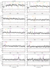 |
Fig. A.1. Mean spectra of LAEs with z ≤ 3.6 and > 3.6 (left and right, respectively). The median values of z for the two subsamples are 3.3 and 4.0, respectively. Lines and symbols as in Fig. 4. |
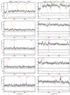 |
Fig. A.2. Mean spectra of LAEs with log10(FLyα/(erg s−1cm−2)) ≤ −17.02 and > − 17.02 (left and right, respectively). The median values of log10(FLyα/(erg s−1cm−2)) for the two subsamples are −17.24 and −16.78, respectively. Lines and symbols as in Fig. 4. |
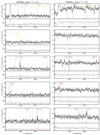 |
Fig. A.3. Mean spectra of LAEs with LyαFWHM ≤ 271 and > 271 km s−1 (left and right, respectively). The median values of the Lyα FWHM for the two subsamples are 222 and 360, respectively. Lines and symbols as in Fig. 4. |
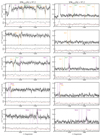 |
Fig. A.4. Mean spectra of LAEs with Lyα EW [Å] ≤97.2 and > 97.2 (left and right, respectively). The median values of the Lyα EW for the two subsamples are 54.7 and 163.1, respectively. Lines and symbols as in Fig. 4. |
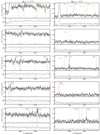 |
Fig. A.5. Mean spectra of LAEs with MUV ≤ −17.9 and > − 17.9 (left and right, respectively). The median values of the MUV for the two subsamples are −18.8 and −17.2, respectively. Lines and symbols as in Fig. 4. |
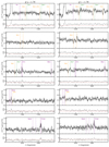 |
Fig. A.6. Mean spectra of LAEs with β ≤ −1.78 and > − 1.78 (left and right, respectively). The median values of β for the two subsamples are −2.07 and −1.40, respectively. Lines and symbols as in Fig. 4. |
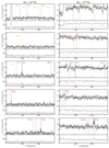 |
Fig. A.7. Mean spectra of LAEs with stellar mass ≤ − 0.32 and > − 0.32 M⊙ (left and right, respectively). The median values of the stellar mass for the two subsamples are 107.9 and 109 M⊙, respectively. Lines and symbols as in Fig. 4. |
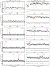 |
Fig. A.8. Mean spectra of LAEs with log10(SFR/(M⊙ yr−1)) ≤ − 0.25 and > − 0.25 (left and right, respectively). The median values of log10(SFR/(M⊙ yr−1)) for the two subsamples are −0.57 and 0.16, respectively. Lines and symbols as in Fig. 4. |
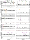 |
Fig. A.9. Mean spectra of LAEs with log10(sSFR/yr−1) ≤ − 8.5 and > − 8.5 (left and right, respectively). The median values of log10(sSFR/yr−1) for the two subsamples are −8.8 and −8.5, respectively. Lines and symbols as in Fig. 4. |
All Tables
Details of the MUSE HUDF LAE subsamples and emission-line EWs measured from the stacked spectra.
All Figures
|
Fig. 1. Distributions of observed and physical properties of the LAE sample described in Sect. 2.1. From panel a–j: redshift, Lyα luminosity, Lyα flux, Lyα FWHM, rest-frame Lyα EW, absolute UV magnitude, UV spectral slope, stellar mass, SFR, and sSFR. The Lyα emission shown here has not been corrected by attenuation from dust. The vertical dashed black line indicates the median value, μ1/2 (reported in the top right), of the distributions used to select the subsamples of Sect. 3.2. The vertical dotted gray lines indicate the median absolute deviation. |
| In the text | |
|
Fig. 2. Distribution of the LAE sample (green stars) in the star formation rate-stellar mass (SFR-M⋆) plane. For comparison, values for 2.4 < z < 5.5 galaxies in the 3D-HST survey public catalog by Momcheva et al. (2016) and data for z ≳ 2 star-forming galaxies from Erb et al. (2010), Patrício et al. (2016), Amorín et al. (2017), Vanzella et al. (2017), and Berg et al. (2018) (see also Sect. 5.2) are shown color-coded as labeled in the legend. The curves of the star formation sequence from Whitaker et al. (2014) at 2 < z < 2.5, main sequence (MS) at 2 < z < 3 from Bisigello et al. (2018), and at 3.9 < z < 4.9 from Caputi et al. (2017) and the starburst (SB) sequence at 3.9 < z < 4.9 from Caputi et al. (2017) are shown for reference. |
| In the text | |
|
Fig. 3. Mean and median spectra of all 220 LAEs described in Sect. 2.1 shown in black and blue with the error displayed via gray and light-blue shaded areas, respectively. The vertical lines indicate the rest-frame wavelengths of some of the main spectral features: nebular emission lines (purple), ISM absorption (orange), and fine-structure transitions (green). The bottom panels show the S/N per pixel (gray and cyan curves for mean and median spectra, respectively) with the dotted red horizontal line indicating S/N = 3. |
| In the text | |
|
Fig. 4. Mean spectra of LAEs with log10(LLyα/(erg s−1)) ≤42.0 and > 42.05 (left and right, respectively) are shown in black in the top panels, with the error budget displayed via the gray shaded regions. The median values of log10(LLyα/(erg s−1)) for the two subsamples are 41.86 and 42.35, respectively. The vertical lines indicate the rest-frame wavelengths of some of the main spectral features: nebular emission lines (purple), ISM absorption (orange), and fine-structure transitions (green). The bottom panels show the S/N per pixel (gray curves) with the dotted red horizontal line indicating S/N = 3. |
| In the text | |
|
Fig. 5. Correlations between shift of Lyα peak and Lyα FWHM obtained from Lyα FWHM subsamples of our LAEs. These correlations were obtained considering the rest wavelengths of C III] (green line) and O III] (orange line) as reference wavelengths and their mean shift (purple line). In gray, Eq. (2) of V18, obtained from object-by-object measurements, and the associated scatter (gray shaded area). |
| In the text | |
|
Fig. 6. EWs of He II, O III]λ1666, [Si III]λ1883, and [C III]λ1907 for the different subsamples of MUSE HUDF LAEs (x-axis). The symbols refer to different emission lines, as labeled in the legend. Smaller and larger symbol sizes indicate the subsample of LAEs whose properties are lower and higher than the median value, respectively. Empty symbols with downward arrows indicate upper limits, while non-detections are shown by the black dash. Red symbols show the EWs for all 220 LAEs in the sample. |
| In the text | |
|
Fig. 7. Zoom-in around the rest wavelengths of the C IVλλ1548,1551 doublet (purple vertical lines) for the different averaged spectra (black lines) of the MUSE HUDF LAEs (as described in the title of each panel). The light blue shading indicates the noise. The other vertical lines indicate the rest-frame wavelengths of the Si IIλ1527 ISM absorption feature (orange) and the SiII*λ1533 fine-structure transition (green). |
| In the text | |
|
Fig. 8. UV emission line properties of MUSE HUDF LAE subsamples and local galaxies from the literature described in Sects. 4.1 and 5.2. The diagrams show different combinations of EWs and ratios of the He II, O III]λ1666, C III], and [C III]λ1907 emission lines. Different black symbols refer to S/N > 2.5 line detections for different LAE subsamples and the red cross to the total LAE sample. Smaller and larger symbols indicate the subsample of LAEs whose property is lower or higher than the median value, respectively. Different colors refer to different samples from the literature, as labelled in the legend. Open and filled symbols indicate upper limits and detections, respectively. The left triangles refer to local galaxies. The gray dashed lines are the separation criteria between AGN and star-forming galaxies from Nakajima et al. (2018b), while the gray dotted lines represent the selection criteria for the AGN, composite, and star-forming galaxies from Hirschmann et al. (2019). |
| In the text | |
|
Fig. 9. Same as Fig. 9. Open and filled symbols indicate upper limits and detections, respectively. The pentagons refer to data for 2 ≤ z ≤ 4 galaxies. |
| In the text | |
|
Fig. A.1. Mean spectra of LAEs with z ≤ 3.6 and > 3.6 (left and right, respectively). The median values of z for the two subsamples are 3.3 and 4.0, respectively. Lines and symbols as in Fig. 4. |
| In the text | |
|
Fig. A.2. Mean spectra of LAEs with log10(FLyα/(erg s−1cm−2)) ≤ −17.02 and > − 17.02 (left and right, respectively). The median values of log10(FLyα/(erg s−1cm−2)) for the two subsamples are −17.24 and −16.78, respectively. Lines and symbols as in Fig. 4. |
| In the text | |
|
Fig. A.3. Mean spectra of LAEs with LyαFWHM ≤ 271 and > 271 km s−1 (left and right, respectively). The median values of the Lyα FWHM for the two subsamples are 222 and 360, respectively. Lines and symbols as in Fig. 4. |
| In the text | |
|
Fig. A.4. Mean spectra of LAEs with Lyα EW [Å] ≤97.2 and > 97.2 (left and right, respectively). The median values of the Lyα EW for the two subsamples are 54.7 and 163.1, respectively. Lines and symbols as in Fig. 4. |
| In the text | |
|
Fig. A.5. Mean spectra of LAEs with MUV ≤ −17.9 and > − 17.9 (left and right, respectively). The median values of the MUV for the two subsamples are −18.8 and −17.2, respectively. Lines and symbols as in Fig. 4. |
| In the text | |
|
Fig. A.6. Mean spectra of LAEs with β ≤ −1.78 and > − 1.78 (left and right, respectively). The median values of β for the two subsamples are −2.07 and −1.40, respectively. Lines and symbols as in Fig. 4. |
| In the text | |
|
Fig. A.7. Mean spectra of LAEs with stellar mass ≤ − 0.32 and > − 0.32 M⊙ (left and right, respectively). The median values of the stellar mass for the two subsamples are 107.9 and 109 M⊙, respectively. Lines and symbols as in Fig. 4. |
| In the text | |
|
Fig. A.8. Mean spectra of LAEs with log10(SFR/(M⊙ yr−1)) ≤ − 0.25 and > − 0.25 (left and right, respectively). The median values of log10(SFR/(M⊙ yr−1)) for the two subsamples are −0.57 and 0.16, respectively. Lines and symbols as in Fig. 4. |
| In the text | |
|
Fig. A.9. Mean spectra of LAEs with log10(sSFR/yr−1) ≤ − 8.5 and > − 8.5 (left and right, respectively). The median values of log10(sSFR/yr−1) for the two subsamples are −8.8 and −8.5, respectively. Lines and symbols as in Fig. 4. |
| In the text | |
Current usage metrics show cumulative count of Article Views (full-text article views including HTML views, PDF and ePub downloads, according to the available data) and Abstracts Views on Vision4Press platform.
Data correspond to usage on the plateform after 2015. The current usage metrics is available 48-96 hours after online publication and is updated daily on week days.
Initial download of the metrics may take a while.