| Issue |
A&A
Volume 641, September 2020
|
|
|---|---|---|
| Article Number | A25 | |
| Number of page(s) | 11 | |
| Section | Stellar structure and evolution | |
| DOI | https://doi.org/10.1051/0004-6361/202037461 | |
| Published online | 01 September 2020 | |
TESS asteroseismology of the known planet host star λ2 Fornacis
1
School of Physics and Astronomy, University of Birmingham, Birmingham B15 2TT, UK
e-mail: m.b.nielsen.1@bham.ac.uk
2
Stellar Astrophysics Centre (SAC), Department of Physics and Astronomy, Aarhus University, Ny Munkegade 120, 8000 Aarhus C, Denmark
3
Center for Space Science, NYUAD Institute, New York University Abu Dhabi, PO Box 129188, Abu Dhabi, UAE
e-mail: mbn4@nyu.edu
4
Department of Chemistry and Physics, Florida Gulf Coast University, 10501 FGCU Blvd., Fort Myers, FL 33965, USA
5
Department of Physics & Astronomy, Vanderbilt University, Nashville, TN 37235, USA
6
Department of Earth and Planetary Sciences, University of California, Riverside, CA 92521, USA
7
School of Physics, University of New South Wales, Kensington, NSW 2033, Australia
8
LESIA, Observatoire de Paris, Université PSL, CNRS, Sorbonne Université, Université de Paris, 92195 Meudon, France
9
Department of Astronomy and Space Sciences, Science Faculty, Ege University, 35100 Bornova, İzmir, Turkey
10
Astronomy Unit, School of Physics and Astronomy, Queen Mary University of London, London E1 4NS, UK
11
Instituto de Astrofísica e Ciências do Espaço, Universidade do Porto, Rua das Estrelas, 4150-762 Porto, Portugal
12
Departamento de Física e Astronomia, Faculdade de Ciências da Universidade do Porto, Rua do Campo Alegre, s/n, 4169-007 Porto, Portugal
13
IRFU, CEA, Université Paris-Saclay, 91191 Gif-sur-Yvette, France
14
AIM, CEA, CNRS, Université Paris-Saclay, Université Paris Diderot, Sorbonne Paris Cité, 91191 Gif-sur-Yvette, France
15
Instituto de Astrofísica de Canarias, La Laguna, Tenerife, Spain
16
Dpto. de Astrofísica, Universidad de La Laguna, La Laguna, Tenerife, Spain
17
Institute of Space Sciences (ICE, CSIC), Carrer de Can Magrans S/N, 08193 Bellaterra, Spain
18
Institut d’Estudis Espacials de Catalunya (IEEC), Carrer Gran Capita 2, 08034 Barcelona, Spain
19
Department of Astronomy, The Ohio State University, Columbus, OH 43210, USA
20
Homi Bhabha Centre for Science Education, TIFR, V. N. Purav Marg, Mankhurd, Mumbai 400088, India
Received:
8
January
2020
Accepted:
15
June
2020
Context. The Transiting Exoplanet Survey Satellite (TESS) is observing bright known planet-host stars across almost the entire sky. These stars have been subject to extensive ground-based observations, providing a large number of radial velocity measurements.
Aims. The objective of this work is to use the new TESS photometric observations to characterize the star λ2 Fornacis, and following this to update the parameters of the orbiting planet λ2 For b.
Methods. We measured the frequencies of the p-mode oscillations in λ2 For, and in combination with non-seismic parameters estimated the stellar fundamental properties using stellar models. Using the revised stellar properties and a time series of archival radial velocities from the UCLES, HIRES and HARPS instruments spanning almost 20 years, we refit the orbit of λ2 For b and searched the residual radial velocities for remaining variability.
Results. We find that λ2 For has a mass of 1.16 ± 0.03 M⊙ and a radius of 1.63 ± 0.04 R⊙, with an age of 6.3 ± 0.9 Gyr. This and the updated radial velocity measurements suggest a mass of λ2 For b of 16.8−1.3+1.2 M⊕, which is ∼5M⊕ less than literature estimates. We also detect an additional periodicity at 33 days in the radial velocity measurements, which is likely due to the rotation of the host star.
Conclusions. While previous literature estimates of the properties of λ2 For are ambiguous, the asteroseismic measurements place the star firmly at the early stage of its subgiant evolutionary phase. Typically only short time series of photometric data are available from TESS, but by using asteroseismology it is still possible to provide tight constraints on the properties of bright stars that until now have only been observed from the ground. This prompts a reexamination of archival radial velocity data that have been accumulated in the past few decades in order to update the characteristics of the planet hosting systems observed by TESS for which asteroseismology is possible.
Key words: asteroseismology / stars: individual: HD 16417 / planetary systems / techniques: radial velocities / techniques: photometric
© ESO 2020
1. Introduction
The Transiting Exoplanet Survey Satellite (TESS, Ricker et al. 2014) observed the southern celestial hemisphere in the period from July 2018 to July 2019. The main objective of TESS is to observe short-period transiting exoplanets around bright stars. The observation strategy during the first year of operations covered almost the entirety of the southern hemisphere, observing large swaths of the sky for short periods of time (≈27 days). This is a departure from the previous space-based photometry missions CoRoT (Fridlund et al. 2006) and Kepler (Borucki et al. 2010), which provided photometric time series of hundreds of days or even several years for a few select fields. These time series have been a huge advantage for asteroseismology, which benefits from long observations and bright stars to make precise measurements of the oscillation modes of a star. The cohort of TESS targets extends to much brighter targets than Kepler and CoRoT, and so despite a lack of long baseline time series, the mission has already yielded a multitude of previously unknown variable stars, including solar-like oscillators.
The star λ2 Fornacis (HD 16417, λ2 For) was initially selected for observation in the TESS two-minute cadence mode based on its brightness (G-band magnitude of 5.59) and high likelihood of exhibiting solar-like oscillations, as indicated by the Asteroseismic Target List (Schofield et al. 2019). It was observed for approximately two months shortly after the beginning of the TESS mission, and is one of the first planet-host stars to be observed by TESS with confirmed solar-like oscillations (see also Huber et al. 2019; Campante et al. 2019). Previous studies of λ2 For have yielded a wide range of physical parameters (e.g., Bond et al. 2006; Gehren 1981; Bensby et al. 2014), indicating a spectral type anywhere between G2V or G8IV. Despite the relatively short amount of time that this star was observed by TESS, the photometric variability shows an unambiguous power excess at a frequency of ≈1280 μHz, caused by solar-like acoustic (p-mode) oscillations. Stars with outer convective zones like the Sun and λ2 For oscillate with regularly spaced overtones of radial and non-radial modes with angular degree, l. These modes propagate through the interior of the star, and therefore place tight constraints on its physical properties (e.g., García & Ballot 2019). The oscillation power of λ2 For peaks at around 1280 μHz, which alone places the star firmly in the subgiant regime. However, going a step further and measuring the individual mode frequencies has been shown to yield estimates of the mass and radius at a precision of a few percent, and the stellar age at ≈10% (e.g., Brown et al. 1994; Lebreton & Goupil 2014; Angelou et al. 2017; Bellinger et al. 2019). This has implications for estimates of the characteristics of any potential orbiting planets, in particular with respect to the mass of the planets, but also in terms of the dynamical history of the system itself.
O’Toole et al. (2009) discovered a roughly Neptune-mass planet in a 17.25-day orbit around λ2 For. The detection was made using radial velocity (RV) measurements from the UCLES spectrograph at the Anglo-Australian Telescope (AAT), and the HIRES spectrograph at the Keck telescope. Since then an extensive set of HARPS (Mayor et al. 2003) data from the ESO La Silla 3.6 m telescope has become publicly available (see Table E.1). Here we combine the original observations by O’Toole et al. (2009) and the HARPS measurements to construct an almost 20-year set of RV data. This, combined with the updated estimates of the stellar mass from asteroseismology, allows us to better constrain the planet and its orbital parameters. Furthermore, the extensive RV data set and the high quality of the HARPS measurements presents an opportunity to investigate variability on timescales other than the orbit of the known planet.
The TESS time series reduction is presented in Sect. 2. The modeling process of λ2 For is described in Sect. 3, including the power spectrum and spectral energy density SED fitting processes, which yields the seismic and non-seismic constraints, respectively. In Sect. 4 we discuss the methods used to improve the estimates of the planet and orbital characteristics of the known planet and the methods used to investigate additional periodicity in the RV measurements.
2. Time series preparation
λ2 For was observed by TESS in Sectors 3 and 4, for a total of approximately 2 months. The photometric time series are available in a pre-reduced version from the Science Processing Operations Center (SPOC) pipeline (Jenkins et al. 2012), and in the form of pixel-level data. The SPOC pipeline removes artifacts and carries out traditional CCD data reduction activities, such as bias correction and flat-fielding, prior to performing aperture photometry. Aperture sizes are computed using the algorithm originally developed for Kepler postage stamps, which makes use of stellar parameters from the TESS Input Catalog (Stassun et al. 2018a) together with models of the detector and spacecraft attitude control system. Following extraction, the presearch data conditioning (PDC) algorithm removes instrumental signatures due to changes in pointing and focus, and performs corrections due to stellar crowding and aperture overfilling by the target star.
We attempted to improve on the SPOC result by manually reducing the pixel-level data. This was done using a procedure that has previously produced better signal-to-noise ratio (S/N) oscillation spectra for asteroseismic analyses of bright stars compared to the standard SPOC pipeline (Metcalfe et al., in prep.). The approach broadly mirrors that used successfully on K2 data in the past (see, e.g., Buzasi et al. 2015), and involved defining a custom photometric aperture pixel mask. In the case of λ2 For this procedure did not reduce the noise level around the p-mode envelope, but for completeness we briefly summarize the method and the result in Appendix A. In the following sections we only use the SPOC PDC time series.
3. Modeling λ2 For
To estimate the fundamental properties of λ2 For we used both seismic and non-seismic constraints. The seismic constraints came from measuring the individual oscillation frequencies observed in the power spectrum of the SPOC time series, also known as peakbagging. The non-seismic constraints were derived from SED fitting. These constraints were then used by several independent modeling teams to provide estimates of the mass, radius, and age of λ2 For. These steps are detailed in the following section.
3.1. Seismic constraints
To measure the oscillation frequencies of λ2 For we used the SPOC flux time series as described above. Because of the low S/N of the oscillations, several independent peakbaggers1 were tasked with finding and fitting the oscillation peaks. Initial guesses for the frequencies were found using the universal pattern approach (see Mosser et al. 2013) and by-eye inspection. The final choice of which modes to fit was based on the subset that all teams agreed on within their respective uncertainties. Each mode alone only has a ∼95% probability of not being due to background noise, whereas this manual approach also incorporates knowledge of the repeating pattern of the p-modes. In a low S/N case like λ2 For, this repeating pattern helps identify the initial mode frequencies. The mode frequencies range from 1142 μHz to 1380 μHz, with a peak of oscillation power at νmax ≈ 1280 μHz and a separation of consecutive overtones of the same angular degree (large separation), Δν ≈ 69 μHz.
The final list of frequencies was then fit using a Markov chain Monte Carlo (MCMC) approach, the result of which was used in the remaining analysis of λ2 For. The model used to fit the power spectrum mirrors that used in previous peakbagging efforts such as Handberg & Campante (2011) or Lund et al. (2017). The mode frequencies and heights were treated as independent variables for each mode, and the mode widths were assumed to follow the relation by Appourchaux et al. (2014). The fit assumed a single rotational splitting and inclination axis for all oscillation modes. The background noise levels from granulation, activity, and uncorrected instrumental effects were fit concurrently with the modes, using two Harvey-like profiles (Harvey et al. 1988; Kallinger et al. 2014). We applied uniform priors on the mode frequencies, background timescales, rotational splitting, inclination angle, and the location parameters of the mode width relation (see Appourchaux et al. 2014). For the remaining model parameters we used log-uniform priors.
The posterior distribution of the model parameters was mapped using an MCMC sampler2. For each model parameter the median of the marginalized posterior distribution was taken as the best-fit solution, and the 16th and 84th percentile interval as a measure of the parameter uncertainties.
The power density spectrum and the resulting fit frequencies are shown in Fig. 1, and the échelle diagram in Fig. 2. Modes of angular degree l = 3 were not considered by any of the teams as these are typically very low amplitude, and thus require exceptional S/N to be observed. One team suggested the possible presence of mixed l = 1, but this could not be verified by the other teams and so they were not included in the final fit. The final list of fit frequencies is presented in Table B.1.
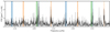 |
Fig. 1. Power density spectrum (gray) and the smoothed spectrum (black) around the p-mode oscillation frequencies. The 68% confidence interval of the fit mode frequencies are shown as the vertical shaded regions. Colors denote the angular degree, l, where blue is l = 0, orange is l = 1, and green is l = 2. |
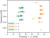 |
Fig. 2. Échelle diagram showing oscillation frequencies modulo the large separation (Δν = 69.0 μHz) supplied by each team: MV (circles), IWR (squares), MBN (diamonds), and WJC (triangles). The colors represent the angular degrees, l, that were considered. The shaded regions represent 68% confidence interval of the frequencies in the final fit. Several mixed modes (diverging modes along the l = 1 ridge) were suggested, but could not be verified by the other teams, and so were not included in the final fit. |
The fit to the power spectrum was unable to constrain the rotational splitting of the modes to less than ≈2.1 μHz, and thus the stellar rotation rate. Similarly, the seismic data were unable to constrain the stellar inclination angle. The marginalized posterior distributions of the inclination angle and rotational splitting are shown in Fig. C.1.
3.2. Stellar modeling
Three teams, identified by their principal locations, independently fit stellar models to the seismic and non-seismic data for λ2 For. The teams independently chose stellar evolution codes, stellar pulsation codes, non-seismic observables, and fitting methods. The main choices of input physics are summarized in Table 1 and the best-fitting parameters of the models, with uncertainties, are listed in Table 2. For the frequencies derived from seismology, all the teams used either the one- or two-term surface correction by Ball & Gizon (2014). We did not enforce a line-of-sight velocity correction as this was negligible for λ2 For (Davies et al. 2014; Soubiran et al. 2018). We describe below more complicated details of the stellar models, and how each team fit their models to the data. Our final estimates of the stellar properties are precise to 3% in mass, 2.7% in radius, and 14% in age.
Stellar model settings for the different teams.
Model parameters for λ2 For using seismic and non-seismic constraints.
3.2.1. Birmingham
The Birmingham team used Modules for Experiments in Stellar Astrophysics (MESA, r10398; Paxton et al. 2011, 2013, 2015) with the atmosphere models and calibrated mixing-length (MLT) parameters from Trampedach et al. (2014a,b) as implemented in Mosumgaard et al. (2018). The mixing-length parameter in Table 1 is the calibrated correction factor that accommodates slight differences between MESA’s input physics and mixing-length model and that of the simulations by Trampedach et al. (2014a,b), rather than the mixing-length parameter αMLT. The free parameters in the fit are the stellar mass M, the initial metallicity [Fe/H]i, and the age t.
The free parameters were optimized by first building a crude grid based on scaling relations, then optimizing the best model from that grid using a combination of a downhill simplex (i.e., Nelder–Mead method, Nelder & Mead 1965) and random resampling within error ellipses around the best-fitting parameters when the simplex stagnated. Uncertainties were estimated by the same procedure as used by Ball & Gizon (2017).
The objective function for the optimization was the unweighted total χ2 of both the seismic and non-seismic data, using observed non-seismic values of Teff, [Fe/H], and L⋆/ L⊙. The Teff = 5841 ± 60 K and [Fe/H] = 0.13 ± 0.06 values were taken from Delgado Mena et al. (2017), with uncertainties increased to those used for most of the stars in Lund et al. (2017). The luminosity was derived from SED fitting following the procedures described in Stassun & Torres (2016), and Stassun et al. (2017, 2018b). The available photometry spans the wavelength range 0.35–22 μm (see Fig. 3). We fit the SED using Kurucz stellar atmosphere models (Kurucz 2013), with the priors on effective temperature Teff, surface gravity log g, and metallicity [Fe/H] from the spectroscopically determined values. The remaining free parameter in the SED fit is the extinction (AV), which we restricted to the maximum line-of-sight value from the dust maps of Schlegel et al. (1998). The best-fit extinction is AV = 0.04 ± 0.04. Integrating the model SED (which is unreddened) gives the bolometric flux at Earth of Fbol = 1.36 ± 0.05 × 10⁻⁷ erg s cm−2. Together with the Gaia parallax of 39.3512 ± 0.0534 mas, this yielded a constraint for the luminosity of log L⋆/ L⊙ = 0.436 ± 0.015.
 |
Fig. 3. Spectral energy distribution of λ2 For. Red symbols represent the observed photometric measurements, where the horizontal bars represent the effective width of the passband. The photometric measurements are BTVT magnitudes from Tycho-2, the BVgri magnitudes from APASS, the JHKS magnitudes from 2MASS, the W1–W4 magnitudes from WISE, and the G magnitude from Gaia. Blue symbols are the model fluxes from the best-fit Kurucz atmosphere model (black). |
3.2.2. Mumbai
The Mumbai team computed a grid of stellar models also using MESA (r10398). The grid spans masses from 1.10 to 1.38 M⊙ in steps of 0.01 M⊙, initial metallicities [Fe/H]i from −0.02 to 0.36 in steps of 0.02, and mixing-length parameters αMLT of 1.81, 1.91, and 2.01. Gravitational settling, which is otherwise included in the stellar models, is disabled for models with M⋆ > 1.3 M⊙, but the best-fitting models are less massive and unaffected by this choice. The grid uses two values for the length scale of core convective overshooting, using the exponentially decaying formulation by Herwig (2000): fov = 0 (i.e., no overshooting) and 0.016.
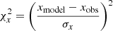
The goodness of fit was evaluated through a total misfit defined by
![$$ \begin{aligned} \chi ^2_\mathrm{Mum} = (\chi ^2_{\,T_\mathrm{eff} } + \chi ^2_{\log g} + \chi ^2_{\,[\mathrm{Fe} /\mathrm{H} ]} + \chi ^2_\nu ) ,\end{aligned} $$](/articles/aa/full_html/2020/09/aa37461-20/aa37461-20-eq2.gif)
where for x = Teff, log g, or [Fe/H]:
and
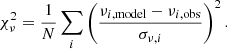
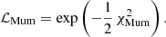
The observed values of the non-seismic data were Teff = 5790 ± 150 K, log g = 4.11 ± 0.06, and [Fe/H] = 0.09 ± 0.11. The reported parameters are likelihood-weighted averages and standard deviations of the likelihood evaluated for each model in the grid, where the unnormalized likelihood is
3.2.3. Porto
The Porto team used Asteroseismic Inference on a Massive Scale (AIMS: Lund & Reese 2018; Rendle et al. 2019) to optimize a grid of stellar models computed with GARSTEC (Weiss & Schlattl 2008). The observed non-seismic values were taken to be Teff = 5792.5 ± 143.5 K, metallicity [Fe/H] = 0.09 ± 0.10, and luminosity L⋆/ L⊙ = 2.71 ± 0.10. The luminosity was determined from the relation by Pijpers (2003) using the extinction correction derived from the SED fit described in Sect. 3.2.1. The masses M in the grid ranged from 0.7 to 1.6 M⊙ in steps of 0.01 M⊙ and the initial metallicity [Fe/H]i ranged from −0.95 to 0.6 in steps of 0.05. The models included extra mixing below the convective envelope according to the prescription by VandenBerg et al. (2012). The efficiency of microscopic diffusion is smoothly decreased to zero from 1.25 to 1.35 M⊙ though, again, the best-fitting models are all significantly below 1.25 M⊙ and therefore not affected by this choice. In addition, a geometric limit is applied for small convective regions, as described in Magic et al. (2010).
The goodness-of-fit function was the unweighted total χ2 of the seismic and non-seismic data, as used by the Birmingham team (Sect. 3.2.1).
3.3. Adopted fundamental stellar parameters
Table 2 includes parameters averaged across the three stellar model fits. Specifically, we took the average and 1σ percentile ranges from the evenly weighted combination of the three fits.
Figure 4 shows the log g and Teff values estimated by each team in relation to the literature values (see also Table D.1). Among the more recent literature sources the estimates of log g span a considerable range of ≈0.2 dex, and a subset of sources reported a mass ranging from  to 1.38 ± 0.12 M⊙, and corresponding radius between 1.45 ± 0.05 R⊙ and 1.61 ± 0.13 R⊙ (see bottom frame of Fig. 4, Valenti & Fischer 2005; Ramírez et al. 2014).
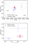 |
Fig. 4. Top: Kiel diagram showing the literature values (purple) and seismic values (red; see Table 2) of λ2 For. Dashed lines indicate evolutionary tracks spanning a mass range of 0.8 − 2 M⊙, in increments of 0.2 M⊙. Literature values are presented in Table D.1. Bottom: masses and radii of the literature sources with a combination of log g with either mass or radius in comparison to the seismic estimates. |
The asteroseismic measurements allow us to obtain robust estimates of the surface gravity, and subsequently of the mass and radius. Despite the inclusion of different model physics and approaches taken by the modeling teams in this work, the resulting estimates all fall within a few percentage points of each other in both mass and radius, with average values of M⋆ = 1.16 ± 0.03 M⊙ and R⋆ = 1.63 ± 0.04 R⊙. There is therefore agreement between the asteroseismic modeling results that λ2 For is at the early stages of the subgiant evolutionary phase, whereas previous estimates were unable to confirm this unambiguously.
The literature estimates of the age (Valenti & Fischer 2005; Tsantaki et al. 2013; Bonfanti et al. 2016) fall within 1 − 2σ of the asteroseismic estimates of 6.3 ± 0.9 Gyr, with the extremes at 4.3 ± 0.8 Gyr (da Silva et al. 2006) and 7.6 ± 0.7 (Nordström et al. 2004).
4. Radial velocity analysis of the λ2 For system
Since the discovery of λ2 For b, a much larger sample of RV measurements has become available from the HARPS spectrometer at the ESO La Silla 3.6 m telescope. This presents an opportunity to update the orbital parameters of the planet based on this new data, and by using the new estimates of the stellar mass from asteroseismology. The HARPS data were downloaded via the ESO Science Portal3. We combined these data with the AAT and Keck data as presented by O’Toole et al. (2009) in Table 2 of that publication.
4.1. Updated characteristics λ2 For b
We used Kima (Faria et al. 2018) to analyze the combined data set. Kima fits a sum of Keplerian curves to RV data corresponding to one or more potential planets. It uses a diffusive nested sampling algorithm (Brewer et al. 2009) to sample the posterior distribution of parameters explaining the data, where in this case the number of planets Np was left as a free parameter. This allowed us to use Kima to estimate the fully marginalized Bayesian evidence of the parameter space, which was used to determine the likelihood of any number of planets that may be present and detectable in the data.
For the analysis of the RV data from λ2 For, Np was set as a free parameter with an upper limit of Np = 5. Once samples of the fit posterior were obtained from Kima any proposed crossing orbits were removed a posteriori. The resulting posterior consists of a wide parameter space with a number of overdensities corresponding to regions of high likelihood for each of the parameters, such as orbital period P, semi-amplitude K, and eccentricity e. We identified these regions with the clustering algorithm HDBSCAN (McInnes et al. 2017). HDBSCAN identified a cluster corresponding to the orbital period of λ2 For b. We extracted these samples from the posterior and used them to approximate the posterior probability density of the planetary orbital and physical parameters. As a result we provide the median of the distribution of each parameter (see Figs. C.2 and C.3), and provide uncertainties estimated from the 16th and 84th percentiles, which are shown in Table 3. The best-fit model is shown in Fig. 5, along with the residual RV signal, which has a standard deviation of σ = 2.64 m s−1.
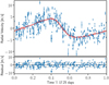 |
Fig. 5. Top: observational RV data (blue) of λ2 For, from AAT, Keck, and HARPS, phase-folded at a period of 17.25 days. The phase-folded best-fit model is shown in red, with the model uncertainties in shaded red. Bottom: residual RV after subtracting the best-fit RV model. The dashed lines indicate the standard deviation, σ = 2.64 m s−1, of the residual. |
Best-fit orbital parameters of λ2 For b.
To verify the Kima results, we also fit the RV data using the exoplanet package (Foreman-Mackey et al. 2019), which, like Kima, also fits Keplerian orbits, but includes the signal from stellar granulation noise as a Gaussian process in the RV model. The exoplanet package uses the celerite library (Foreman-Mackey et al. 2017) to model any variability in the RV signal that can be represented as a stationary Gaussian process. The choice of kernel for the Gaussian process was set by the quality factor which we here chose to be Q = 1/2 to represent a stochastically excited damped harmonic oscillator with a characteristic timescale w0 and amplitude S0. We applied a normal prior on w0 based on the modeling of the TESS power spectrum presented in Sect. 3 as the granulation timescale is expected to be identical in both radial velocity and photometric variability. The granulation power in the TESS intensity spectrum is not easily converted to a radial velocity signal as seen from multiple different instruments, we therefore use a weakly-informative log-normal prior on S0. We found that the Kima and exoplanet results were consistent within 1σ.
4.2. Additional radial velocity variability
O’Toole et al. (2009) suggested the presence of a periodicity at ≈298 days, which they ultimately did not attribute to the presence of an additional planet. The posterior distribution of the fit parameters obtained from Kima indeed shows a periodicity at ≈300 days, but the Bayesian evidence does not support the added model complexity that comes from adding a planet at or near this orbital period. This was quantified by calculating the Bayes factor (the ratio of evidence weighted probabilities, Kass & Raftery 1995) for an increase in the number of planets from Np = 1, i.e., assuming only λ2 For b exists, to Np = 2 (see Fig. C.2). This yielded a Bayes factor of ≈1.67, which is “not worth more than a bare mention” (Kass & Raftery 1995). This was found to be the case when testing both just the AAT and Keck data set, and with the added HARPS data.
However, using the combined data sets highlights a period at ≈33 days. Figure 6 shows the periodogram of the RV measurements, where the signal due to λ2 For b is visible at P = 17.25 days, with surrounding aliases caused by the observational window function. The 33-day periodicity shows aliasing in the RV, but also appears in the bisector span, which in addition shows harmonic peaks at a period of ≈16.5 days. This signal was not discussed by O’Toole et al. (2009), and so to investigate this periodicity further we established two scenarios: first, that it is due to another planet in a wider orbit than the known planet or second, that it is due to variability induced by magnetic activity on the stellar surface.
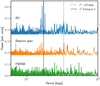 |
Fig. 6. Periodograms of the HARPS RV data (blue), the spectral line bisector span (orange), and the cross-correlation function full-width at half maximum (FWHM, green). The FWHM and bisector span were only available for the HARPS data, and so the AAT and Keck data are not included in the power spectra shown here. The full vertical line shows the period of λ2 For b, and the dashed line is the secondary 33-day periodicity. The comb of peaks around the orbital period of λ2 For b are caused by the observational window function, as is the case for many of the peaks around the 33-day periodicity. |
4.2.1. Scenario 1: An additional planet
In the first scenario we consider that the 33-day signal is due to an additional planet in the λ2 For system. From Fig. 6 a bisector span variation is apparent at this period, which is a strong indication that the signal is not a planet (see, e.g., Queloz et al. 2001). In addition, we used Kima to evaluate the possibility of a planet in such an orbit, but the Bayesian evidence for the additional planet remains small. This in itself would suggest that the existence of a second planet is unlikely but as a final belts-and-braces measure we tested the dynamical stability of such a planet to investigate whether it could survive on timescales comparable to the ≈6.3 Gyr lifetime of the λ2 For system.
The dynamical simulations were performed using the REBOUND package4, described in detail by Rein & Liu (2012), and using the WHFast integrator (Rein & Tamayo 2015). REBOUND computes the Mean Exponential Growth factor of Nearby Orbits (MEGNO, Maffione et al. 2011), which is a chaos indicator on a logarithmic scale that quantifies the divergence of a test particle placed in relation to known orbiting planet, in this case λ2 For b. These techniques have been applied to a range of exoplanetary systems (Goździewski et al. 2001; Goździewski 2002; Satyal et al. 2013, 2014; Triaud et al. 2017; Kane 2019).
Figure 7 shows the results of our dynamical simulation, where the MEGNO values are presented as a function of eccentricity and orbital period. MEGNO values ≲2 indicate very likely stable orbits, while values ≳2 are either approaching instability (chaos), or for MEGNO ≫2 have already diverged at the end of the simulation. The simulations were run for 105 orbits of λ2 For b, equivalent to ≈4700 years, where the configuration seen in Fig. 7 was reached after just a few hundred orbits. Figure 7 also shows the marginalized posterior distribution of the eccentricity and period obtained from Kima, for the 33-day periodicity. The range of periods is narrower than the symbol size (see Table 3), but the eccentricity spans a wide range. None of the orbits within the period range have MEGNO values ≲2, indicating that any orbit at this period would be unstable. A number of very narrow stable regions appear at multiple different periods. These are all likely due to resonances with λ2 For b. However, none fall near the 33-day periodicity, excluding the possibility that a planet in this orbit could be stable due to a resonance.
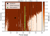 |
Fig. 7. Stability map (MEGNO) for a particle at different periods and inclinations, in the presence of the known planet λ2 For b. The color bar indicates the linear scale of the MEGNO statistic, for which darker colors represent a higher degree of orbital divergence (chaos) on timescales of 105 orbits of λ2 For b. Lighter shaded regions denote stable orbits. The upper range of the color bar has been truncated at a MEGNO value of 4 for clarity. The marginalized posterior distribution of the 33-day orbit is shown in green, with the median indicated by the square symbol. Orbits in resonance with λ2 For b are indicated by vertical dashed lines. Additional resonances are not marked for clarity. The solid black square denotes the period and eccentricity of λ2 For b. |
4.2.2. Scenario 2: Stellar activity
O’Toole et al. (2009) did not discus the 33-day RV variability; however, they estimated a rotation period of the star of 22 − 33 days, based on the measured  and the age-activity relation by Wright et al. (2004). Estimates of the projected rotational velocity v sin i in the literature fall in the range 2.1 − 2.5 km s−1 (Nordström et al. 2004; Valenti & Fischer 2005; Ammler-von Eiff & Reiners 2012), which is consistent with a rotation period of 33 days when assuming a stellar radius of 1.63 R⊙ and an inclined rotation axis on the order of i ≈ 50° relative to the line of sight to the observer.
While the asteroseismic fit included the rotation rate and inclination of the rotation axis of the star as free variables, the marginalized posteriors for these parameters (see Fig. C.1) could only constrain the rotation rate to ≲2.1 μHz. This is likely in part due to the low frequency resolution of the power spectrum (0.2 μHz) compared to the expected slow rotation rate of the star (≈0.36 μHz). Measuring rotation rates from the oscillation modes may also be further hampered by a very low angle of inclination of the rotation axis relative to the observer.
No signatures of star spots are visible in the TESS photometry, either in the SPOC or manually reduced light curves (see Fig. A.1), which might also be expected for a star with a low inclination angle and low activity level.
If this signal is indeed due to rotation, a similar period is expected in the spectral line bisector, and in some cases in the full width at half maximum (FWHM) of the cross-correlation function used to measure the RV (e.g., Dumusque et al. 2012; Gomes da Silva et al. 2012). In the case of λ2 For the power spectra of the HARPS RV data and the bisector span (see Fig. 6) show a power excess at around 33 days, but the FWHM spectrum does not show any clear peaks at this period. Furthermore, no significant correlation was found between the residual RV, after removing the signal from λ2 For b, and the bisector span where a negative correlation is in some cases an indication that the bisector span variation is caused by stellar activity (Huélamo et al. 2008; Queloz et al. 2009).
Using the gyrochronology relation by Barnes (2003), with the asteroseismic ages from Sect. 3 and a B − V = 0.66 (Ducati 2002) as input, we find that the rotation period of the star is likely between Prot = 27 − 31 days. While correcting the B − V estimate for interstellar reddening decreases this estimated period range, we note that the Barnes (2003) relation is only calibrated for young main-sequence stars and does not account for structural evolution that occurs after stars leave the main sequence. This is expected to increase the surface rotation period as the radius of the stellar envelope increases after the main sequence (see, e.g., Fig. 3 in van Saders et al. 2016).
5. Discussion and conclusions
We used the recent release of TESS photometric data to perform an asteroseismic analysis of the star λ2 For. This allowed us to place tighter constraints on the stellar parameters than has previously been possible. We measured individual oscillation mode frequencies of the star centered at ≈1280 μHz, which were then distributed to several modeling teams. Using different approaches and input physics each team returned estimates of the physical properties of the star that were consistent to within 1 − 2σ, suggesting that the application of asteroseismic constraints produces more robust estimates of the stellar properties. For the mass and radius, which are typically well constrained by asteroseismology (Lebreton & Goupil 2014; Stokholm et al. 2019), we adopted the overall values M⋆ = 1.16 ± 0.03 M⊙ and R⋆ = 1.63 ± 0.04 R⊙. Together with a surface temperature of Teff = 5829 ± 80 K. Previous literature estimates suggest λ2 For could be anything from an early G dwarf to a late G-type subgiant; however, multiple modeling teams using asteroseismic constraints all place the star firmly at the start of the subgiant phase of its evolution.
The age of the system was less well constrained, despite the seismic constraint, with an estimate of 6.3 ± 0.9 Gyr, with most literature values falling within this range. This is likely due to the correlation with the other model parameters, where particularly the mass and metallicity are important for estimating the age. In our case the uncertainty on the mass estimate is caused in part by the uncertainty on the mode frequencies due to the relativity short TESS time series, while the metallicity is taken from spectroscopic values in the literature.
Following this we revisited the analysis of λ2 For b originally performed by O’Toole et al. (2009), who discovered the Neptune-like planet. We combined the radial velocity measurements from the original publication with the now public HARPS measurements, yielding an RV time series spanning approximately 20 years. Combining this with the asteroseismic mass estimate, reduces the lower mass limit of λ2 For b from mp sin i = 22.1 ± 2.0M⊕ to 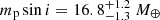 . The majority of this reduction is due to the long RV time series, which alone sets a lower limit of mp sin i = 17.2 ± 1.3 M⊕. The stellar mass found here using asteroseismology is ∼3% lower than that used by O’Toole et al. (2009), and as such reduces the lower limit on the planet by a similar amount.
The orbital eccentricity was also found to be significantly higher at e = 0.35 ± 0.05, as opposed to the previous estimate of e = 0.20 ± 0.09. We estimate the circularization timescale due to tidal interaction following an expression derived in Barker & Ogilvie (2009) and find it to be ≈1120 Gyr, which is much longer than the age of the system. The slightly higher eccentricity found here is then perhaps more consistent with this long circularization timescale, compared to the original estimate, which at a 2σ level encompasses almost circular orbits.
In addition to the revised parameters for λ2 For b, the larger set of RV measurements also revealed a periodicity at 33 days. Despite the relatively low activity level of the star, this periodicity is more likely due to stellar rotation when compared to the case of an additional unknown planet being present in the system. Although difficult to confirm, the former scenario is consistent with the expected rotation rate of an old inactive star like λ2 For, and we showed that the latter scenario is not possible as such an orbit would be unstable after ∼103 years. Assuming then that the 33-day RV signal is indeed due to rotation, the relatively short 17.25 day orbit of λ2 For b means that tidal interaction with the host star will cause the planet to gradually spiral inward into the star. Using the relation by Barker & Ogilvie (2009) we can estimate the current infall timescale to be on the order of 103 − 104 Gyr. This is obviously much longer than the evolutionary timescale of the host star, and so the time when the star expands to the current periastron of λ2 For b (0.1 AU, 21.5 R⊙) sets an upper limit for when the planet will be engulfed. The models presented in Sect. 3.2 suggest that this will happen in approximately 1.5 Gyr. However, the tidal interaction, and thus the in-fall timescale, is a strong function of the stellar radius and the orbital period (Barker & Ogilvie 2009). This will cause the in-fall to accelerate considerably over time and the planet will likely be engulfed well before λ2 For expands to the current orbit.
Despite the rather modest time series that was obtained from TESS for λ2 For, we have shown that it is still possible to measure the individual oscillation frequencies of the star. Moreover, using these frequencies, multiple modeling teams find consistent results on the percent level for the mass and radius of λ2 For. This shows that asteroseismology is a useful tool for obtaining robust constraints on these stellar parameters, for the enormous selection of stars being observed by TESS, which previously has only been possible for select areas of the sky like those observed by CoRoT and Kepler. This new and much wider range of stars that TESS is observing prompts the reexamination of the wealth of archival radial velocity data that has been accumulated in the last few decades for planet hosting systems, in order to better characterize these systems.
emcee: Foreman-Mackey et al. (2013).
The HARPS data set was collected thanks to several observing programs listed in Appendix E.1, and were obtained from: https://archive.eso.org/scienceportal/home?data_release_date=*:2019-09-18pos=39.2442,-34.57798r=0.016667poly=39.318719,-34.614387,39.169781,-34.614387,39.169846,-34.541445,39.318654,-34.541445dp_type=SPECTRUMsort=dist,-fov,-obs_dates=P%2fDSS2%2fcolorf=0.122541fc=39.318654,-34.541445cs=J2000av=trueac=falsec=8,9,10,11,12,13,14,15,16,17,18ta=RESdts=truesdtm=%7b%22SPECTRUM%22%3atrue%7dat=39.2442,-34.57798
Acknowledgments
The authors would like to thank J. P. Faria and H. Rein for useful discussions. This paper includes data collected by the TESS mission. MBN, WHB, MRS, AHMJT, and WJC acknowledge support from the UK Space Agency. AHMJT and MRS have benefited from funding from the European Research Council (ERC) under the European Union’s Horizon 2020 research and innovation programme (grant agreement no 803193/BEBOP). Funding for the Stellar Astrophysics Centre is funded by the Danish National Research Foundation (Grant agreement no.: DNRF106). ZÇO, MY, and SÖ acknowledge the Scientific and Technological Research Council of Turkey (TÜBİTAK:118F352). AS acknowledges support from grants ESP2017-82674-R (MICINN) and 2017-SGR-1131 (Generalitat Catalunya). TLC acknowledges support from the European Union’s Horizon 2020 research and innovation programme under the Marie Skłodowska-Curie grant agreement No. 792848 (PULSATION). This work was supported by FCT/MCTES through national funds (UID/FIS/04434/2019). MD is supported by FCT/MCTES through national funds (PIDDAC) by this grant UID/FIS/04434/2019. MD and MV are supported by FEDER - Fundo Europeu de Desenvolvimento Regional through COMPETE2020 - Programa Operacional Competitividade e Internacionalização by these grants: UID/FIS/04434/2019; PTDC/FIS-AST/30389/2017 & POCI-01-0145-FEDER-030389 & POCI-01-0145-FEDER03038. MD is supported in the form of a work contract funded by national funds through Fundação para a Ciência e Tecnologia (FCT). SM acknowledges support by the Spanish Ministry with the Ramon y Cajal fellowship number RYC-2015-17697. BM and RAG acknowledge the support of the CNES/PLATO grant. DLB and LC acknowledge support from the TESS GI Program under awards 80NSSC18K1585 and 80NSSC19K0385. LGC thanks the support from grant FPI-SO from the Spanish Ministry of Economy and Competitiveness (MINECO) (research project SEV-2015-0548-17-2 and predoctoral contract BES-2017-082610). Funding for the TESS mission is provided by the NASA Explorer Program. Based in part on data acquired at the Anglo-Australian Telescope. We acknowledge the traditional owners of the land on which the AAT stands, the Gamilaraay people, and pay our respects to elders past and present. The data presented herein were in part obtained at the W. M. Keck Observatory, which is operated as a scientific partnership among the California Institute of Technology, the University of California and the National Aeronautics and Space Administration. The Observatory was made possible by the generous financial support of the W. M. Keck Foundation. The authors wish to recognize and acknowledge the very significant cultural role and reverence that the summit of Maunakea has always had within the indigenous Hawaiian community.
References
- Adelberger, E. G., García, A., Robertson, R. G. H., et al. 2011, Rev. Mod. Phys., 83, 195 [NASA ADS] [CrossRef] [Google Scholar]
- Ammler-von Eiff, M., & Reiners, A. 2012, A&A, 542, A116 [NASA ADS] [CrossRef] [EDP Sciences] [Google Scholar]
- Angelou, G. C., Bellinger, E. P., Hekker, S., & Basu, S. 2017, ApJ, 839, 116 [Google Scholar]
- Appourchaux, T., Antia, H. M., Benomar, O., et al. 2014, A&A, 566, A20 [NASA ADS] [CrossRef] [EDP Sciences] [Google Scholar]
- Ball, W. H., & Gizon, L. 2014, A&A, 568, A123 [NASA ADS] [CrossRef] [EDP Sciences] [Google Scholar]
- Ball, W. H., & Gizon, L. 2017, A&A, 600, A128 [NASA ADS] [CrossRef] [EDP Sciences] [Google Scholar]
- Barker, A. J., & Ogilvie, G. I. 2009, MNRAS, 395, 2268 [NASA ADS] [CrossRef] [Google Scholar]
- Barnes, S. A. 2003, ApJ, 586, 464 [NASA ADS] [CrossRef] [Google Scholar]
- Battistini, C., & Bensby, T. 2015, A&A, 577, A9 [NASA ADS] [CrossRef] [EDP Sciences] [Google Scholar]
- Bellinger, E. P., Hekker, S., Angelou, G. C., Stokholm, A., & Basu, S. 2019, A&A, 622, A130 [NASA ADS] [CrossRef] [EDP Sciences] [Google Scholar]
- Bensby, T., Feltzing, S., & Lundström, I. 2003, A&A, 410, 527 [NASA ADS] [CrossRef] [EDP Sciences] [Google Scholar]
- Bensby, T., Feltzing, S., & Oey, M. S. 2014, A&A, 562, A71 [NASA ADS] [CrossRef] [EDP Sciences] [Google Scholar]
- Bertran de Lis, S., Delgado Mena, E., Adibekyan, V. Z., Santos, N. C., & Sousa, S. G. 2015, A&A, 576, A89 [NASA ADS] [CrossRef] [EDP Sciences] [Google Scholar]
- Bond, J. C., Tinney, C. G., Butler, R. P., et al. 2006, MNRAS, 370, 163 [NASA ADS] [CrossRef] [EDP Sciences] [Google Scholar]
- Bonfanti, A., Ortolani, S., & Nascimbeni, V. 2016, A&A, 585, A5 [NASA ADS] [CrossRef] [EDP Sciences] [Google Scholar]
- Borucki, W. J., Koch, D., Basri, G., et al. 2010, Science, 327, 977 [NASA ADS] [CrossRef] [PubMed] [Google Scholar]
- Brewer, B. J., Pártay, L. B., & Csányi, G. 2009, Stat. Comput., 21, 649 [CrossRef] [Google Scholar]
- Brown, T. M., Christensen-Dalsgaard, J., Weibel-Mihalas, B., & Gilliland, R. L. 1994, ApJ, 427, 1013 [NASA ADS] [CrossRef] [Google Scholar]
- Buzasi, D. L., Carboneau, L., Hessler, C., Lezcano, A., & Preston, H. 2015, IAU Gen. Assembly, 29, 2256843 [NASA ADS] [Google Scholar]
- Campante, T. L., Corsaro, E., Lund, M. N., et al. 2019, ApJ, 885, 31 [Google Scholar]
- Carretta, E. 2013, A&A, 557, A128 [NASA ADS] [CrossRef] [EDP Sciences] [Google Scholar]
- da Silva, L., Girardi, L., Pasquini, L., et al. 2006, A&A, 458, 609 [NASA ADS] [CrossRef] [EDP Sciences] [Google Scholar]
- Datson, J., Flynn, C., & Portinari, L. 2015, A&A, 574, A124 [NASA ADS] [CrossRef] [EDP Sciences] [Google Scholar]
- Davies, G. R., Handberg, R., Miglio, A., et al. 2014, MNRAS, 445, L94 [NASA ADS] [CrossRef] [Google Scholar]
- Delgado Mena, E., Tsantaki, M., Adibekyan, V. Z., et al. 2017, A&A, 606, A94 [NASA ADS] [CrossRef] [EDP Sciences] [Google Scholar]
- Ducati, J. R. 2002, VizieR Online Data Catalog:II/237 [Google Scholar]
- Dumusque, X., Pepe, F., Lovis, C., et al. 2012, Nature, 491, 207 [NASA ADS] [CrossRef] [PubMed] [Google Scholar]
- Faria, J. P., Santos, N. C., Figueira, P., & Brewer, B. J. 2018, J. Open Source Soft., 3, 487 [Google Scholar]
- Ferguson, J. W., Alexander, D. R., Allard, F., et al. 2005, ApJ, 623, 585 [NASA ADS] [CrossRef] [Google Scholar]
- Foreman-Mackey, D., Hogg, D. W., Lang, D., & Goodman, J. 2013, PASP, 125, 306 [CrossRef] [Google Scholar]
- Foreman-Mackey, D., Agol, E., Ambikasaran, S., & Angus, R. 2017, AJ, 154, 220 [NASA ADS] [CrossRef] [Google Scholar]
- Foreman-Mackey, D., Czekala, I., Luger, R., et al. 2019, dfm/exoplanet v0.2.3 [Google Scholar]
- Fridlund, M., Baglin, A., Lochard, J., & Conroy, L. 2006, in The CoRoT Mission Pre-Launch Status - Stellar Seismology and Planet Finding, ESA Spec. Publ., 1306 [Google Scholar]
- García, R. A., & Ballot, J. 2019, Liv. Rev. Sol. Phys., 16, 4 [Google Scholar]
- Gehren, T. 1981, A&A, 100, 97 [NASA ADS] [Google Scholar]
- Gomes da Silva, J., Santos, N. C., Bonfils, X., et al. 2012, A&A, 541, A9 [NASA ADS] [CrossRef] [EDP Sciences] [Google Scholar]
- Goździewski, K. 2002, A&A, 393, 997 [NASA ADS] [CrossRef] [EDP Sciences] [Google Scholar]
- Goździewski, K., Bois, E., Maciejewski, A. J., & Kiseleva-Eggleton, L. 2001, A&A, 378, 569 [NASA ADS] [CrossRef] [EDP Sciences] [Google Scholar]
- Gray, R. O., Corbally, C. J., Garrison, R. F., et al. 2006, AJ, 132, 161 [NASA ADS] [CrossRef] [Google Scholar]
- Grevesse, N., & Noels, A. 1993, in Origin and Evolution of the Elements, eds. N. Prantzos, E. Vangioni-Flam, & M. Casse, 15 [Google Scholar]
- Handberg, R., & Campante, T. L. 2011, A&A, 527, A56 [NASA ADS] [CrossRef] [EDP Sciences] [Google Scholar]
- Harvey, J. W., Hill, F., Kennedy, J. R., Leibacher, J. W., & Livingston, W. C. 1988, Adv. Space Res., 8, 117 [CrossRef] [Google Scholar]
- Hearnshaw, J. B., & Schmidt, E. G. 1972, A&A, 21, 111 [Google Scholar]
- Herwig, F. 2000, A&A, 360, 952 [NASA ADS] [Google Scholar]
- Huber, D., Chaplin, W. J., Chontos, A., et al. 2019, AJ, 157, 245 [Google Scholar]
- Huélamo, N., Figueira, P., Bonfils, X., et al. 2008, A&A, 489, L9 [NASA ADS] [CrossRef] [EDP Sciences] [Google Scholar]
- Iglesias, C. A., & Rogers, F. J. 1993, ApJ, 412, 752 [NASA ADS] [CrossRef] [Google Scholar]
- Iglesias, C. A., & Rogers, F. J. 1996, ApJ, 464, 943 [NASA ADS] [CrossRef] [Google Scholar]
- Irwin, A. W. 2012, FreeEOS: Equation of State for Stellar Interiors Calculations [Google Scholar]
- Jenkins, J. M., Twicken, J. D., McCauliff, S., et al. 2012, in The TESS Science Processing Operations Center, SPIE Conf. Ser., 9913, 99133E [NASA ADS] [Google Scholar]
- Kallinger, T., De Ridder, J., Hekker, S., et al. 2014, A&A, 570, A41 [NASA ADS] [CrossRef] [EDP Sciences] [Google Scholar]
- Kane, S. R. 2019, AJ, 158, 72 [NASA ADS] [CrossRef] [Google Scholar]
- Kass, R. E., & Raftery, A. E. 1995, J. Am. Stat. Assoc., 90, 773 [CrossRef] [Google Scholar]
- Krishna Swamy, K. S. 1966, ApJ, 145, 174 [NASA ADS] [CrossRef] [Google Scholar]
- Kurucz, R. L. 2013, ATLAS12: Opacity Sampling Model Atmosphere Program [Google Scholar]
- Lebreton, Y., & Goupil, M. J. 2014, A&A, 569, A21 [NASA ADS] [CrossRef] [EDP Sciences] [Google Scholar]
- Lund, M. N., & Reese, D. R. 2018, Asteroseismology and Exoplanets: Listening to the Stars and Searching for New Worlds, 49, 149 [Google Scholar]
- Lund, M. N., Silva Aguirre, V., Davies, G. R., et al. 2017, ApJ, 835, 172 [CrossRef] [Google Scholar]
- Maffione, N. P., Giordano, C. M., & Cincotta, P. M. 2011, Int. J. Non Linear Mech., 46, 23 [NASA ADS] [CrossRef] [Google Scholar]
- Magic, Z., Serenelli, A., Weiss, A., & Chaboyer, B. 2010, ApJ, 718, 1378 [NASA ADS] [CrossRef] [Google Scholar]
- Mayor, M., Pepe, F., Queloz, D., et al. 2003, The Messenger, 114, 20 [NASA ADS] [Google Scholar]
- McInnes, L., Healy, J., & Astels, S. 2017, J. Open Source Soft., 2 [Google Scholar]
- Mosser, B., Michel, E., Belkacem, K., et al. 2013, A&A, 550, A126 [NASA ADS] [CrossRef] [EDP Sciences] [Google Scholar]
- Mosumgaard, J. R., Ball, W. H., Silva Aguirre, V., Weiss, A., & Christensen-Dalsgaard, J. 2018, MNRAS, 478, 5650 [NASA ADS] [CrossRef] [Google Scholar]
- Nason, G. 2006, Stationary and non-stationary time series, eds. H. Mader, & S. Coles (UK: Geological Society of London), 129 [Google Scholar]
- Nelder, J. A., & Mead, R. 1965, Comput. J., 7, 308 [Google Scholar]
- Nordström, B., Mayor, M., Andersen, J., et al. 2004, A&A, 418, 989 [NASA ADS] [CrossRef] [EDP Sciences] [Google Scholar]
- O’Toole, S., Tinney, C. G., Butler, R. P., et al. 2009, ApJ, 697, 1263 [NASA ADS] [CrossRef] [Google Scholar]
- Paxton, B., Bildsten, L., Dotter, A., et al. 2011, ApJ, 192, 3 [Google Scholar]
- Paxton, B., Cantiello, M., Arras, P., et al. 2013, ApJS, 208, 4 [NASA ADS] [CrossRef] [Google Scholar]
- Paxton, B., Marchant, P., Schwab, J., et al. 2015, ApJS, 220, 15 [Google Scholar]
- Pijpers, F. P. 2003, A&A, 400, 241 [NASA ADS] [CrossRef] [EDP Sciences] [Google Scholar]
- Prša, A., Zhang, M., & Wells, M. 2019, PASP, 131, 068001 [NASA ADS] [CrossRef] [Google Scholar]
- Queloz, D., Henry, G. W., Sivan, J. P., et al. 2001, A&A, 379, 279 [NASA ADS] [CrossRef] [EDP Sciences] [Google Scholar]
- Queloz, D., Bouchy, F., Moutou, C., et al. 2009, A&A, 506, 303 [NASA ADS] [CrossRef] [EDP Sciences] [Google Scholar]
- Ramírez, I., Meléndez, J., & Asplund, M. 2014, A&A, 561, A7 [NASA ADS] [CrossRef] [EDP Sciences] [Google Scholar]
- Rein, H., & Liu, S. F. 2012, A&A, 537, A128 [NASA ADS] [CrossRef] [EDP Sciences] [Google Scholar]
- Rein, H., & Tamayo, D. 2015, MNRAS, 452, 376 [NASA ADS] [CrossRef] [Google Scholar]
- Rendle, B. M., Buldgen, G., Miglio, A., et al. 2019, MNRAS, 484, 771 [NASA ADS] [CrossRef] [Google Scholar]
- Ricker, G. R., Winn, J. N., & Vanderspek, R. 2014, in Space Telescopes and Instrumentation 2014: Optical, Infrared, and Millimeter Wave, Proc. SPIE, 9143, 914320 [Google Scholar]
- Rogers, F. J., & Nayfonov, A. 2002, ApJ, 576, 1064 [Google Scholar]
- Satyal, S., Quarles, B., & Hinse, T. C. 2013, MNRAS, 433, 2215 [NASA ADS] [CrossRef] [Google Scholar]
- Satyal, S., Hinse, T. C., Quarles, B., & Noyola, J. P. 2014, MNRAS, 443, 1310 [NASA ADS] [CrossRef] [Google Scholar]
- Schlegel, D. J., Finkbeiner, D. P., & Davis, M. 1998, ApJ, 500, 525 [NASA ADS] [CrossRef] [Google Scholar]
- Schofield, M., Chaplin, W. J., Huber, D., et al. 2019, ApJS, 241, 12 [Google Scholar]
- Soubiran, C., Jasniewicz, G., Chemin, L., et al. 2018, A&A, 616, A7 [NASA ADS] [CrossRef] [EDP Sciences] [Google Scholar]
- Sousa, S. G., Santos, N. C., Israelian, G., Mayor, M., & Monteiro, M. J. P. F. G. 2006, A&A, 458, 873 [NASA ADS] [CrossRef] [EDP Sciences] [Google Scholar]
- Sousa, S. G., Santos, N. C., Mayor, M., et al. 2008, A&A, 487, 373 [NASA ADS] [CrossRef] [EDP Sciences] [MathSciNet] [Google Scholar]
- Stassun, K. G., & Torres, G. 2016, AJ, 152, 180 [Google Scholar]
- Stassun, K. G., Collins, K. A., & Gaudi, B. S. 2017, AJ, 153, 136 [NASA ADS] [CrossRef] [Google Scholar]
- Stassun, K. G., Oelkers, R. J., Pepper, J., et al. 2018a, AJ, 156, 102 [NASA ADS] [CrossRef] [Google Scholar]
- Stassun, K. G., Corsaro, E., Pepper, J. A., & Gaudi, B. S. 2018b, AJ, 155, 22 [NASA ADS] [CrossRef] [Google Scholar]
- Stokholm, A., Nissen, P. E., Silva Aguirre, V., et al. 2019, MNRAS, 489, 928 [Google Scholar]
- Thoul, A. A., Bahcall, J. N., & Loeb, A. 1994, ApJ, 421, 828 [NASA ADS] [CrossRef] [Google Scholar]
- Townsend, R. H. D., & Teitler, S. A. 2013, MNRAS, 435, 3406 [NASA ADS] [CrossRef] [Google Scholar]
- Townsend, R. H. D., Goldstein, J., & Zweibel, E. G. 2018, MNRAS, 475, 879 [Google Scholar]
- Trampedach, R., Stein, R. F., Christensen-Dalsgaard, J., Nordlund, Å., & Asplund, M. 2014a, MNRAS, 442, 805 [NASA ADS] [CrossRef] [Google Scholar]
- Trampedach, R., Stein, R. F., Christensen-Dalsgaard, J., Nordlund, Å., & Asplund, M. 2014b, MNRAS, 445, 4366 [NASA ADS] [CrossRef] [Google Scholar]
- Triaud, A. H. M. J., Neveu-VanMalle, M., Lendl, M., et al. 2017, MNRAS, 467, 1714 [NASA ADS] [Google Scholar]
- Tsantaki, M., Sousa, S. G., Adibekyan, V. Z., et al. 2013, A&A, 555, A150 [NASA ADS] [CrossRef] [EDP Sciences] [Google Scholar]
- Valenti, J. A., & Fischer, D. A. 2005, ApJS, 159, 141 [NASA ADS] [CrossRef] [MathSciNet] [Google Scholar]
- Vanderburg, A., & Johnson, J. A. 2014, PASP, 126, 948 [NASA ADS] [CrossRef] [Google Scholar]
- VandenBerg, D. A., Bergbusch, P. A., Dotter, A., et al. 2012, ApJ, 755, 15 [NASA ADS] [CrossRef] [Google Scholar]
- van Saders, J. L., Ceillier, T., Metcalfe, T. S., et al. 2016, Nature, 529, 181 [NASA ADS] [CrossRef] [PubMed] [Google Scholar]
- Weiss, A., & Schlattl, H. 2008, Ap&SS, 316, 99 [NASA ADS] [CrossRef] [Google Scholar]
- Wright, J. T., Marcy, G. W., Butler, R. P., & Vogt, S. S. 2004, ApJS, 152, 261 [NASA ADS] [CrossRef] [Google Scholar]
Appendix A: Manual time series reduction
For each TESS orbit we extracted a time series for each pixel and took the brightest pixel as our initial time series. The pixel time series quality figure of merit was parameterized by 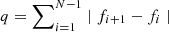 , where f is the flux at cadence i, and N is the length of the time series. Using the first differences of the light curve acts to whiten the time series, and thus correct for its non-stationary nature (Nason et al. 2006); similar approaches have been used in astronomical time series analysis by Buzasi et al. (2015) and Prša et al. (2019), among others.
We then iteratively added the flux of the pixels surrounding the brightest pixel. The process continued until the light curve quality stopped improving, and the resulting pixel collection was adopted as our aperture mask. The light curve produced by our aperture mask was then detrended against the centroid pixel coordinates by fitting a second-order polynomial with cross terms. Similar approaches have been used for K2 data reduction (see, e.g., Vanderburg & Johnson 2014).
Figure A.1 shows the resulting time series, compared to that derived by the SPOC. In this case, low-frequency noise was somewhat improved over the SPOC light curve product, but noise levels at the frequencies near the stellar oscillation spectrum were not. We accordingly used the SPOC light curve for the analysis outlined above.
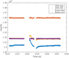 |
Fig. A.1. Resulting counts over time for different TESS data reduction pipelines. The Buzasi Corr time series very effectively removes most of the long-period variability; however, the SPOC time series still shows the lowest variance in the frequency range around the p-mode envelope. |
Appendix B: Peakbagging frequencies
Oscillation frequencies ν with angular degree l of λ2 For.
Appendix C: Posterior distributions
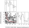 |
Fig. C.1. Corner plot of the rotational splitting and inclination angle posterior distributions from the seismic fit, consisting of 105 samples. The marginalized posterior distributions are shown in the diagonal frames. The dashed vertical lines show the 16th, 50th, and 84th percentiles of the distributions at |

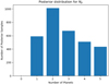 |
Fig. C.2. Marginalized posterior of the Np parameter in the Kima fit to the RV measurements of λ2 For. The number of samples in each bin corresponds to the likelihood, while the ratio of the height of each bin indicates the Bayes factor of one configuration over another. Comparing the cases of Np = 0 and Np = 1 the Bayes factor is effectively infinite, indicating that there is at least one planet in the system. In contrast, the ratio between Np = 2 and Np = 1 is low, with a Bayes factor of 1.67, suggesting that there is little evidence to support a two-planet configuration. |
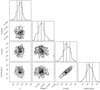 |
Fig. C.3. Corner plot of the orbital parameters from the Kima fit: the eccentricity e, the orbital period P, velocity semi-amplitude K, and the projected planet mass M. |
Appendix D: Stellar properties literature values
Literature sources for Teff and log g values shown in Fig. 4.
Appendix E: HARPS observing programs
HARPS observing program PIs and IDs for data used in this work.
All Tables
All Figures
|
Fig. 1. Power density spectrum (gray) and the smoothed spectrum (black) around the p-mode oscillation frequencies. The 68% confidence interval of the fit mode frequencies are shown as the vertical shaded regions. Colors denote the angular degree, l, where blue is l = 0, orange is l = 1, and green is l = 2. |
| In the text | |
|
Fig. 2. Échelle diagram showing oscillation frequencies modulo the large separation (Δν = 69.0 μHz) supplied by each team: MV (circles), IWR (squares), MBN (diamonds), and WJC (triangles). The colors represent the angular degrees, l, that were considered. The shaded regions represent 68% confidence interval of the frequencies in the final fit. Several mixed modes (diverging modes along the l = 1 ridge) were suggested, but could not be verified by the other teams, and so were not included in the final fit. |
| In the text | |
|
Fig. 3. Spectral energy distribution of λ2 For. Red symbols represent the observed photometric measurements, where the horizontal bars represent the effective width of the passband. The photometric measurements are BTVT magnitudes from Tycho-2, the BVgri magnitudes from APASS, the JHKS magnitudes from 2MASS, the W1–W4 magnitudes from WISE, and the G magnitude from Gaia. Blue symbols are the model fluxes from the best-fit Kurucz atmosphere model (black). |
| In the text | |
|
Fig. 4. Top: Kiel diagram showing the literature values (purple) and seismic values (red; see Table 2) of λ2 For. Dashed lines indicate evolutionary tracks spanning a mass range of 0.8 − 2 M⊙, in increments of 0.2 M⊙. Literature values are presented in Table D.1. Bottom: masses and radii of the literature sources with a combination of log g with either mass or radius in comparison to the seismic estimates. |
| In the text | |
|
Fig. 5. Top: observational RV data (blue) of λ2 For, from AAT, Keck, and HARPS, phase-folded at a period of 17.25 days. The phase-folded best-fit model is shown in red, with the model uncertainties in shaded red. Bottom: residual RV after subtracting the best-fit RV model. The dashed lines indicate the standard deviation, σ = 2.64 m s−1, of the residual. |
| In the text | |
|
Fig. 6. Periodograms of the HARPS RV data (blue), the spectral line bisector span (orange), and the cross-correlation function full-width at half maximum (FWHM, green). The FWHM and bisector span were only available for the HARPS data, and so the AAT and Keck data are not included in the power spectra shown here. The full vertical line shows the period of λ2 For b, and the dashed line is the secondary 33-day periodicity. The comb of peaks around the orbital period of λ2 For b are caused by the observational window function, as is the case for many of the peaks around the 33-day periodicity. |
| In the text | |
|
Fig. 7. Stability map (MEGNO) for a particle at different periods and inclinations, in the presence of the known planet λ2 For b. The color bar indicates the linear scale of the MEGNO statistic, for which darker colors represent a higher degree of orbital divergence (chaos) on timescales of 105 orbits of λ2 For b. Lighter shaded regions denote stable orbits. The upper range of the color bar has been truncated at a MEGNO value of 4 for clarity. The marginalized posterior distribution of the 33-day orbit is shown in green, with the median indicated by the square symbol. Orbits in resonance with λ2 For b are indicated by vertical dashed lines. Additional resonances are not marked for clarity. The solid black square denotes the period and eccentricity of λ2 For b. |
| In the text | |
|
Fig. A.1. Resulting counts over time for different TESS data reduction pipelines. The Buzasi Corr time series very effectively removes most of the long-period variability; however, the SPOC time series still shows the lowest variance in the frequency range around the p-mode envelope. |
| In the text | |
|
Fig. C.1. Corner plot of the rotational splitting and inclination angle posterior distributions from the seismic fit, consisting of 105 samples. The marginalized posterior distributions are shown in the diagonal frames. The dashed vertical lines show the 16th, 50th, and 84th percentiles of the distributions at |
| In the text | |
|
Fig. C.2. Marginalized posterior of the Np parameter in the Kima fit to the RV measurements of λ2 For. The number of samples in each bin corresponds to the likelihood, while the ratio of the height of each bin indicates the Bayes factor of one configuration over another. Comparing the cases of Np = 0 and Np = 1 the Bayes factor is effectively infinite, indicating that there is at least one planet in the system. In contrast, the ratio between Np = 2 and Np = 1 is low, with a Bayes factor of 1.67, suggesting that there is little evidence to support a two-planet configuration. |
| In the text | |
|
Fig. C.3. Corner plot of the orbital parameters from the Kima fit: the eccentricity e, the orbital period P, velocity semi-amplitude K, and the projected planet mass M. |
| In the text | |
Current usage metrics show cumulative count of Article Views (full-text article views including HTML views, PDF and ePub downloads, according to the available data) and Abstracts Views on Vision4Press platform.
Data correspond to usage on the plateform after 2015. The current usage metrics is available 48-96 hours after online publication and is updated daily on week days.
Initial download of the metrics may take a while.