| Issue |
A&A
Volume 640, August 2020
|
|
|---|---|---|
| Article Number | A113 | |
| Number of page(s) | 9 | |
| Section | Stellar structure and evolution | |
| DOI | https://doi.org/10.1051/0004-6361/202038292 | |
| Published online | 25 August 2020 | |
The flux-weighted gravity-luminosity relation of Galactic classical Cepheids⋆
Koninklijke Sterrenwacht van België, Ringlaan 3, 1180 Brussels, Belgium
e-mail: This email address is being protected from spambots. You need JavaScript enabled to view it.
Received:
29
April
2020
Accepted:
22
June
2020
Abstract
The flux-weighted gravity-luminosity relation (FWGLR) is investigated for a sample of 477 classical Cepheids (CCs), including stars that have been classified in the literature as such but are probably not. The luminosities are taken from the literature, based on the fitting of the spectral energy distributions (SEDs) assuming a certain distance and reddening. The flux-weighted gravity (FWG) is taken from gravity and effective temperature determinations in the literature based on high-resolution spectroscopy. There is a very good agreement between the theoretically predicted and observed FWG versus pulsation period relation that could serve in estimating the FWG (and log g) in spectroscopic studies with a precision of 0.1 dex. As was known in the literature, the theoretically predicted FWGLR relation for CCs is very tight and is not very sensitive to metallicity (at least for LMC and solar values), rotation rate, and crossing of the instability strip. The observed relation has a slightly different slope and shows more scatter (0.54 dex). This is due both to uncertainties in the distances and to the pulsation phase averaged FWG values. Data from future Gaia data releases should reduce these errors, and then the FWGLR could serve as a powerful tool in Cepheid studies.
Key words: stars: distances / stars: fundamental parameters / stars: variables: Cepheids
Full Table A.3 is only available at the CDS via anonymous ftp to cdsarc.u-strasbg.fr (130.79.128.5) or via http://cdsarc.u-strasbg.fr/viz-bin/cat/J/A+A/640/A113
© ESO 2020
1. Introduction
Classical Cepheids (CCs) are considered an important standard candle because they are bright, and thus they comprise a link between the distance scale in the nearby universe and that further out via those galaxies that contain both Cepheids and SNIa (see Riess et al. 2019 for a determination of the Hubble constant to 1.9% precision, taking into account the new 1.1% precise distance to the Large Magellanic Cloud from Pietrzyński et al. 2019).
This is the third paper in a series on Galactic CCs based on the Gaia second data release (GDR2, Gaia Collaboration 2018). Groenewegen (2018) (hereafter G18) started from an initial sample of 452 Galactic CCs with accurate [Fe/H] abundances from spectroscopic analysis. Based on parallax data from Gaia DR2, supplemented with accurate non-Gaia parallax data when available, a final sample of about 200 FU mode Cepheids with good astrometric solutions was retained to derive period-luminosity (PL) and period-luminosity-metallicity (PLZ) relations. The influence of a parallax zeropoint offset on the derived PL(Z) relation is large and means that the current GDR2 results do not allow to improve on the existing calibration of the relation or on the distance to the LMC (as also concluded by Riess et al. 2018). The zeropoint, the slope of the period dependence, and the metallicity dependence of the PL(Z) relations are correlated with any assumed parallax zeropoint offset.
In Groenewegen (2020) (hereafter G20) the sample was expanded to 477 stars. Using photometry over the widest available range in wavelength (and at mean light when available) the spectral energy distributions (SEDs) were constructed and fitted with model atmospheres (and a dust component when required). For an adopted distance and reddening these fits resulted in a best-fitting bolometric luminosity (L) and the photometrically derived effective temperature (Teff). This allowed for the derivation of period-radius (PR) and PL relations, the construction of the Hertzsprung-Russell diagram (HRD), and a comparison to theoretical instability strips (ISs). The position of most stars in the HRD was consistent with theoretical predictions. Outliers were often associated with sources where the spectroscopically and photometrically determined effective temperatures differed, or with sources with large and uncertain reddenings.
In this paper the relation between bolometric absolute magnitude and the flux-weighted gravity (FWG),  , is investigated: the so-called flux-weighted gravity-luminosity relation (FWGLR). The tight correlation between gF and luminosity was first demonstrated by Kudritzki et al. (2003, 2008) for blue supergiants, and was then used for extragalactic distance determinations in Kudritzki et al. (2016). Anderson et al. (2016) demonstrated that theoretical pulsation models for CCs also followed a tight FWGLR, in fact tighter than the PL relation, and that there was a good correspondence between observed gF and period for a sample of CCs. The latest calibration of the FWGLR is presented in Kudritzki et al. (2020) based on 445 stars ranging from Mbol = +9.0 to −8.0.
The paper is structured as follows. In Sect. 2 the theoretical models of Anderson et al. (2016) are compared to the latest calibration in Kudritzki et al. (2020). In Sect. 3 the sample of 477 (candidate) CCs is introduced and the gF are derived, and the correlation with period and luminosity are presented. A brief discussion and summary concludes the paper.
2. Theoretical FWGLR for CCs
The FWG is defined as log gF = log g − 4 ⋅ log(Teff/104) (Kudritzki et al. 2003). Kudritzki et al. (2020) present the latest calibration of the FWG against absolute bolometric magnitude as
 (1)
(1)
for  and
and
 (2)
(2)
for  , with a scatter of 0.17 and 0.29 mag, respectively. The break in the relation is set at
  , while the FWG of the Sun is
  .
.
Anderson et al. (2016) presented a large set of pulsation models for CCs based on stellar evolutionary models for a range of initial masses (1.7−15 M⊙), initial rotation rates (ωini = 0.0, 0.5, 0.9 in terms of the critical rotation rates), metallicities (Z = 0.002, 0.006, 0.014), and for fundamental mode (FU) and first overtone (FO) CCs. Stellar parameters (L, Teff), and pulsation periods are given at the entry and exit of the IS for various crossings. They used these models to show the tight FWGLR for CCs for the first time (Fig. 16 in Anderson et al. 2016).
The top panel in Fig. 1 shows the theoretical FWGLR based on these models for FU pulsators with periods > 0.6 d, FO pulsators with periods > 0.4 d, Z = 0.006 and 0.014, and all rotation rates and crossings of the IS as the coloured lines and symbols. Also shown are Eqs. (1) and (2). For the lower gravities the models deviate from Eq. (2), and appear to be closer to an extension of Eq. (1). A linear fit to these models gives the relation
 (3)
(3)
with an rms of 0.16 mag, shown as the green line in the figure. Additional fits are given in Appendix A.
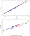 |
Fig. 1. Top panel: FWGLR based on the pulsation models in Anderson et al. (2016). FU models are shown in red, FO models are shown in blue. For clarity FU (FO) models are plotted with an offset of +0.05 (−0.05) dex in Mbol. Symbols indicate the entry point of the IS, the lines connect it to the exit point of the IS. The first, second, and third crossing models are plotted as circles, squares, and triangles, respectively. Solar metallicity models are plotted with open symbols, models with Z = 0.006 with filled symbols. The black lines refer to Eqs. (1) and (2), the green line to the best fit (Eq. (3)). Bottom panel: relation between FWG and period for the same models. The period of the FO models was fundamentalised. The green line refers to the best fit, Eq. (4). |
The bottom panel shows the relation between FWG and period for the same selection of models (cf. Fig. 17 in Anderson et al. 2016, 2020). Periods of FO models are fundamentalised using the relation P0 = P1/(0.716−0.027 log P1) following Feast & Catchpole (1997). The best fit is
 (4)
(4)
with an rms of 0.09 dex. Eliminating the second crossing models would result in a fit with a smaller scatter, but as this information is not known a priori the relation as presented is more generally applicable when an estimate of log gF is desired. Figures and relations for FU and FO models separately are presented in the appendix.
3. Sample and observed FWGs
The sample studied here is the collection of 477 stars considered in G20. It is based on the original sample of 452 stars compiled in G18, extended by 25 additional stars for which accurate iron abundances have since become available, including five CCs in the inner disk of our Galaxy (Inno et al. 2019).
G20 constructed the SEDs for these stars, considering photometry from the ultraviolet to the far-infrared, and as much as possible at mean light. Distances and reddening were collected from the literature. Distances from GDR2 data was available for 232 sources, and from other parallax data for 26 stars.
Luck (2018) (hereafter L18) published a list of abundances and stellar parameters for 435 Cepheids based on the analysis of 1137 spectra. L18 reduced all data in a uniform way using MARCS LTE model atmospheres (Gustafsson et al. 2008). Effective temperatures were determined in that paper using the line depth ratio (LDR) – effective temperature calibration of Kovtyukh (2007) as updated by Kovtyukh (2010, priv. comm. to Luck), while gravities were determined from the ionisation balance between Fe I and Fe II lines, and micro-turbulent velocities (vt) by forcing there to be no dependence in the per-line Fe I abundances on equivalent width (see L18 for additional details).
Table 1 contains information on the set of 52 CCs for which five or more spectra were available in L18 taken at different phases in the pulsation cycle. FWGs are calculated on the one hand from the mean effective temperatures and mean gravities (as given by L18 in his Table 11), and on the other hand from an analysis of the FWGs calculated for the individual epochs and plotted versus phase. Using the code PERIOD04 (Lenz & Breger 2005) to fit a low-order harmonic, this gives the mean log gF, the amplitude of the log gF curve, and the rms value. Some log gF phased curves with fits are shown in Fig. 2.
FWGL data for the subsample with more than five spectra.
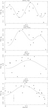 |
Fig. 2. FWG vs pulsation phase for four CCs. The typical error bar in each point is 0.15 dex in FWG, as indicated in the bottom plot. The lines are low-order harmonic fits to the data (see Col. 7 in Table 1). |
These curves show considerable scatter even when the pulsation cycle is well sampled. This is likely due to the error bar in an individual determination of gF. The error on effective temperature generally has a negligible contribution in this. Ninety-five percent of individual effective temperature error bars among the 1137 spectra in L18 are between 30 and 220 K with a median of 65 K. An error of 100 K at Teff = 6000 K introduces an error of 0.03 dex in gF, much smaller than the error on log g, which was estimated to be ∼0.15 dex by L18. A comparison of log gF values determined from the averages of the effective temperatures and gravities, and from fitting the log gF curve with phase show essentially the same result, especially when seven of more spectra are averaged (with an average difference between Cols. 6 and 8 of −0.02 ± 0.04 dex).
Figure 3 shows the FWGLR for the sample of 52 stars from Table 1, where the luminosity and error are taken from G20. Equations (1)–(3) are plotted as reference. Using a linear bi-sector fit (using the code SIXLIN from Isobe et al. 1990) the best fit is
 (5)
(5)
with an rms of 0.38 mag (blue line in the figure). A standard least-squares fit has a shallower slope of 2.54. The theoretical fit is shown in Eq. (3), and this fit differs by about 0.4 mag at log gF = 2.5. Alternatively, the observed log gF values are systematically too small by 0.4/2.8 ∼ 0.14 dex. At lower FWG or longer periods the difference with the theoretical relation is larger.
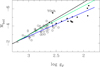 |
Fig. 3. FWGLR based on the subsample with more than five spectra. FU mode pulsators are plotted as circles (filled circles for periods over 10 days), FO pulsators as open squares, the single second-overtone pulsator as open triangle. The black lines refer to Eqs. (1) and (2), the green line to Eq. (3). The blue line is a fit to the data points, excluding Y Oph (Eq. (5)). |
Table A.3 collects the FWG data for the entire sample of 477 stars. Overall, most of the data (435 stars) come from L18, and for the remaining stars log g and Teff have been collected from the literature in order to calculate log gF. Multiple determinations of log gF have been averaged and so can differ slightly from the values in Table 1. The table also includes the period, pulsation type, distance with error, and luminosity with error from G20. Figure 4 shows the observational equivalent to the bottom panel in Fig. 1, the FWG determined from spectroscopy against pulsation period (fundamentalised for FO pulsators).
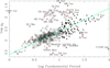 |
Fig. 4. FWG vs fundamental pulsation period. Some outliers are named. The green line refers to the best fit, Eq. (6), which excludes the outliers and non-CCs indicated by a red cross. |
There is a tight correlation between the two quantities. Removing non-CCs (see Table A.3) and applying iterative 3σ clipping results in the fit
 (6)
(6)
with an rms of 0.16 dex, in very good agreement with the theoretically predicted relation. Interestingly, many of the outliers come from a single source, Genovali et al. (2014), who derived very low log g values for some objects. Some additional information and fits are provided in Appendix A.
Figure 5 is the equivalent to Fig. 3 for the entire sample, using a simple averaging of the available FWGs. The error on distance is now taken into account in calculating the error on luminosity. Following the discussion above and in the appendix, the data from Genovali et al. (2014) has been excluded, and to reduce the scatter only stars with two or more spectra are considered. A linear bi-sector fit applying iterative 3σ clipping results in
 (7)
(7)
with an rms of 0.54 mag using 170 stars and is shown as the blue line in the figure. This is currently the best observational determination of the FWGL relation for CCs.
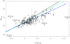 |
Fig. 5. FWGLR, with some outliers named. The black lines refer to Eqs. (1) and (2), the green line to Eq. (3). The blue line refers to the best fit, Eq. (7), which excludes the outliers and non-CCs indicated by a red cross. Outliers located outside the plot window are SU Cru (log gF = 0.19, Mbol = −3.7), SY Nor (log gF = 2.4, Mbol = +3.3), and V382 Car (log gF = 1.8, Mbol = −8.6). |
4. Discussion and summary
The relation between FWG and period, and FWG and bolometric luminosity is investigated for a sample 477 CCs. The FWGs are derived from effective temperatures and log g values available in the literature based on high-resolution spectroscopy. The overall majority of parameters have been compiled from a single source (L18) that determined log g and Teff in an uniform manner. For a subset of stars multiple-phase data is available. The FWG-Period and FWGLR are compared to theoretical models from Anderson et al. (2016)
A very good agreement is found between the theoretical and observed relations between FWG and period. These relations could serve as a prediction for a reasonable range in log g values (assuming an effective temperature) in a spectroscopic analysis.
The observed FWGLR is found to have a shallower slope than the theoretical relation. It is not clear at the moment if this is a significant effect or not. As the observed relation between FWG and period agrees with the theoretical relation, one would be inclined to think that there could be a systematic effect in the bolometric magnitudes of the long-period Cepheids. They are rarer and on average at longer distance, likely to be more susceptible to (systematic) errors on parallax. This is qualitatively confirmed by repeating the fit of Eq. (6) restricting the sample to stars with σL/L < 0.2. The slope is increased, but has a larger error bar (3.05 ± 0.19) and the rms is reduced to 0.44 mag.
On the other hand, although the Teff determinations based on the LDR method are precise (as discussed earlier), possible systematic effects (which would also affect the determination of log g and log gF) could play a role (Mancino et al. 2020). For the subsample of 52 stars in L18 with five or more spectra, the cycle averaged Teffs (as quoted in Table 1) are compared to the photometrically derived Teffs based on the SED fitting in G20. The errors on the photometrically derived effective temperatures (the median is 180 K) are larger than those derived from spectroscopy. There are two outliers Y Oph and S Vul, where the photometrically derived temperatures are considerably lower than those quoted in L18 (570 and 830 K; > 4.3σ). For the other stars the difference (spectroscopically – photometrically derived Teff) is 140 ± 150 K.
Systematic errors on the determination of the gravity could also play a role. The methodology used by L18 to determine the stellar parameters, in particular vt and gravity, is the standard one. A non-standard method is sometimes also used in the literature, as introduced by Kovtyukh & Andrievsky (1999). To avoid non-LTE-sensitive stronger Fe I lines, vt is derived from Fe II lines and weak Fe I lines alone. This leads to higher vt, which in turn leads to higher gravities when the ionisation balance is enforced. For δ Cep Kovtyukh & Andrievsky (1999) find that the gravities are higher by 0.5 dex using the non-standard method. The matter is also debated in Yong et al. (2006). They note that the non-standard method “has merits”, but show that their derived gravities using the standard method are self-consistent, one argument being that this gravity also produces ionisation equilibrium for Ti I lines that are more susceptible to non-LTE effects than Fe. The non-standard method is also used in Takeda et al. (2013). Anderson et al. (2016) excluded the gravities from that paper as they differed from other sources they used. Twelve stars overlap with the sample of stars with multi-epoch data from L18 (in Table 1). Takeda et al. (2013) present stellar parameters at between 7 and 17 epochs. The mean effective temperatures and mean gravities are calculated, as well are FWGs at these epochs based on the data in Takeda et al. (2013), and fitted with low-order harmonic sine curves, as before, to give the mean FWG. The difference (min−max (mean)) between the parameters from the non-standard method minus those from the standard method are −8 − +444 (167) K in Teff, +0.22 − +0.72 (+0.36) dex in log g, and +0.11 − +0.67 (+0.34) dex in FWG, with tendencies that the difference in all three quantities decreases with increasing period.
The FWGLR has the potential to be an alternative to the PL relation in distance determination (Anderson et al. 2016). In its current empirically best calibrated version it is not. The scatter of 0.54 mag is larger than the 0.40 mag in the bolometric PL relation determined in G20 using the identical sample of stars, distances, and luminosities.
One issue is that the independent variable period is known with great precision, while the independent variable FWG has a non-negligible error associated with it. The fitting of the FWG versus pulsation phase did not provide more precise mean FWGs than simple averaging. As the slope of the FWGLR is reasonably steep, any uncertainty on the FWG leads to a three times larger uncertainty in Mbol.
The discussion above also demonstrates that the stellar parameters should be derived in a uniform way. To exclude the influence of data analysis inhomogeneity altogether, Eq. (7) was re-determined using data only from L18. The usable sample is reduced to 161 stars and the slope and offset change marginally, less than 1σ. The standard approach used by L18 seems to give consistent results when considering the comparison to theory and the independent calibration of the FWGLR by Kudritzki et al. (2020). Changes in the FWG by ∼ + 0.3−0.5 dex, as implied by the non-standard method, would result in a disagreement.
This paper is written with the tremendous potential offered by Gaia in mind. Future data releases will provide information that will impact and improve on the results obtained here. Primarily, improved parallaxes, taking into account binarity in the astrometrical solution, will provide more precise distances and thus bolometric luminosities (e.g. through the SED fitting performed in G20).
Secondly, Gaia RVS spectra and GaiaBP/RP spectro-photometry will provide estimates of the stellar parameters (log g, Teff, also metallicity) in future releases. Only mean spectra in data release 3, and epoch spectra in data release 4 (Brown 2019). An older analysis by Recio-Blanco et al. (2016) indicate that end-of-mission accuracies in log g of 0.1 dex or better can be reached in intermediate-metallicity F and G giants of magnitude G ∼ 10.3−11.8 or brighter. Spectro-photometry can go fainter but with poorer accuracies (0.2−0.4 dex in log g down to G = 19; Table 4 in Bailer-Jones et al. 2013). As the nominal mission of 5 years is extended, by +18 months until the end of 2020, and likely until the end of 2022, these numbers should improve. In conclusion, the FWGLR could prove to become an extremely useful tool in Cepheid studies.
Acknowledgments
I would like to thank Dr. Bertrand Lemasle for interesting discussion on the determination of log g and commenting on a draft version of this paper. This research has made use of the SIMBAD database and the VizieR catalogue access tool operated at CDS, Strasbourg, France.
References
- Anders, F., Khalatyan, A., Chiappini, C., et al. 2019, A&A, 628, A94 [NASA ADS] [CrossRef] [EDP Sciences] [Google Scholar]
- Anderson, R. I., Saio, H., Ekström, S., Georgy, C., & Meynet, G. 2016, A&A, 591, A8 [NASA ADS] [CrossRef] [EDP Sciences] [Google Scholar]
- Anderson, R. I., Saio, H., Ekström, S., Georgy, C., & Meynet, G. 2020, A&A, 638, C1 [CrossRef] [EDP Sciences] [Google Scholar]
- Andrievsky, S. M., Kovtyukh, V. V., & Usenko, I. A. 1994, A&A, 281, 465 [Google Scholar]
- Andrievsky, S. M., Kovtyukh, V. V., Luck, R. E., et al. 2002a, A&A, 392, 491 [NASA ADS] [CrossRef] [EDP Sciences] [Google Scholar]
- Andrievsky, S. M., Kovtyukh, V. V., Luck, R. E., et al. 2002b, A&A, 381, 32 [NASA ADS] [CrossRef] [EDP Sciences] [Google Scholar]
- Andrievsky, S. M., Luck, R. E., Martin, P., & Lépine, J. R. D. 2004, A&A, 413, 159 [NASA ADS] [CrossRef] [EDP Sciences] [Google Scholar]
- Andrievsky, S. M., Lépine, J. R. D., Korotin, S. A., et al. 2013, MNRAS, 428, 3252 [NASA ADS] [CrossRef] [Google Scholar]
- Andrievsky, S. M., Martin, R. P., Kovtyukh, V. V., Korotin, S. A., & Lépine, J. R. D. 2016, MNRAS, 461, 4256 [NASA ADS] [CrossRef] [Google Scholar]
- Bailer-Jones, C. A. L., Andrae, R., Arcay, B., et al. 2013, A&A, 559, A74 [NASA ADS] [CrossRef] [EDP Sciences] [Google Scholar]
- Boyarchuk, A. A., & Lyubimkov, L. S. 1981, Bull. Crim. Astrophys. Obs., 64, 1 [Google Scholar]
- Brown, A. G. A. 2019, https://doi.org/10.5281/zenodo.2637972 [Google Scholar]
- Feast, M. W., & Catchpole, R. M. 1997, MNRAS, 286, L1 [NASA ADS] [CrossRef] [Google Scholar]
- Gaia Collaboration (Brown, A. G. A., et al.) 2018, A&A, 616, A1 [NASA ADS] [CrossRef] [EDP Sciences] [Google Scholar]
- Genovali, K., Lemasle, B., Bono, G., et al. 2014, A&A, 566, A37 [NASA ADS] [CrossRef] [EDP Sciences] [Google Scholar]
- Groenewegen, M. A. T. 2018, A&A, 619, A8 [NASA ADS] [CrossRef] [EDP Sciences] [Google Scholar]
- Groenewegen, M. A. T. 2020, A&A, 635, A33 [EDP Sciences] [Google Scholar]
- Gustafsson, B., Edvardsson, B., Eriksson, K., et al. 2008, A&A, 486, 951 [NASA ADS] [CrossRef] [EDP Sciences] [Google Scholar]
- Inno, L., Urbaneja, M. A., Matsunaga, N., et al. 2019, MNRAS, 482, 83 [Google Scholar]
- Isobe, T., Feigelson, E. D., Akritas, M. G., & Babu, G. J. 1990, ApJ, 364, 104 [NASA ADS] [CrossRef] [EDP Sciences] [Google Scholar]
- Kovtyukh, V. V. 2007, MNRAS, 378, 617 [NASA ADS] [CrossRef] [Google Scholar]
- Kovtyukh, V. V., & Andrievsky, S. M. 1999, A&A, 351, 597 [NASA ADS] [Google Scholar]
- Kovtyukh, V. V., Wallerstein, G., & Andrievsky, S. M. 2005, PASP, 117, 1173 [NASA ADS] [CrossRef] [Google Scholar]
- Kudritzki, R. P., Bresolin, F., & Przybilla, N. 2003, ApJ, 582, L83 [NASA ADS] [CrossRef] [Google Scholar]
- Kudritzki, R.-P., Urbaneja, M. A., Bresolin, F., et al. 2008, ApJ, 681, 269 [NASA ADS] [CrossRef] [Google Scholar]
- Kudritzki, R. P., Castro, N., Urbaneja, M. A., et al. 2016, ApJ, 829, 70 [NASA ADS] [CrossRef] [Google Scholar]
- Kudritzki, R.-P., Urbaneja, M. A., & Rix, H.-W. 2020, ApJ, 890, 28 [CrossRef] [Google Scholar]
- Lemasle, B., François, P., Bono, G., et al. 2007, A&A, 467, 283 [NASA ADS] [CrossRef] [EDP Sciences] [Google Scholar]
- Lemasle, B., François, P., Piersimoni, A., et al. 2008, A&A, 490, 613 [NASA ADS] [CrossRef] [EDP Sciences] [Google Scholar]
- Lemasle, B., Kovtyukh, V., Bono, G., et al. 2015, A&A, 579, A47 [NASA ADS] [CrossRef] [EDP Sciences] [Google Scholar]
- Lenz, P., & Breger, M. 2005, Commun. Asteroseismol., 146, 53 [NASA ADS] [CrossRef] [Google Scholar]
- Luck, R. E. 2018, AJ, 156, 171 [NASA ADS] [CrossRef] [Google Scholar]
- Luck, R. E., Gieren, W. P., Andrievsky, S. M., et al. 2003, A&A, 401, 939 [NASA ADS] [CrossRef] [EDP Sciences] [Google Scholar]
- Luck, R. E., Kovtyukh, V. V., & Andrievsky, S. M. 2006, AJ, 132, 902 [NASA ADS] [CrossRef] [Google Scholar]
- Mancino, S., Romaniello, M., Anderson, R. I., & Kudritzki, R. P. 2020, ArXiv e-prints [arXiv:2001.05881] [Google Scholar]
- Martin, R. P., Andrievsky, S. M., Kovtyukh, V. V., et al. 2015, MNRAS, 449, 4071 [NASA ADS] [CrossRef] [Google Scholar]
- Pietrzyński, G., Graczyk, D., Gallenne, A., et al. 2019, Nature, 567, 200 [Google Scholar]
- Recio-Blanco, A., de Laverny, P., Allende Prieto, C., et al. 2016, A&A, 585, A93 [NASA ADS] [CrossRef] [EDP Sciences] [Google Scholar]
- Riess, A. G., Casertano, S., Yuan, W., et al. 2018, ApJ, 861, 126 [Google Scholar]
- Riess, A. G., Casertano, S., Yuan, W., Macri, L. M., & Scolnic, D. 2019, ApJ, 876, 85 [NASA ADS] [CrossRef] [Google Scholar]
- Romaniello, M., Primas, F., Mottini, M., et al. 2008, A&A, 488, 731 [NASA ADS] [CrossRef] [EDP Sciences] [Google Scholar]
- Schmidt, E. G., Rogalla, D., & Thacker-Lynn, L. 2011, AJ, 141, 53 [CrossRef] [Google Scholar]
- Takeda, Y., Kang, D. I., Han, I., Lee, B. C., & Kim, K. M. 2013, MNRAS, 432, 769 [NASA ADS] [CrossRef] [Google Scholar]
- Watson, C. L., Henden, A. A., & Price, A. 2006, Soc. Astron. Sci. Annu. Symp., 25, 47 [Google Scholar]
- Yong, D., Carney, B. W., Teixera de Almeida, M. L., & Pohl, B. L. 2006, AJ, 131, 2256 [NASA ADS] [CrossRef] [Google Scholar]
Appendix A: Additional material
Additional fits for the FWGLR based on the models of Anderson et al. (2016) are given in Table A.1 for the three different metallicities, and with the slope fixed to the value in Eq. (3). The results for Z = 0.006 and 0.014 agree within the error and justify the use of a single relation combining the two metallicities (Eq. (3)). The Z = 0.002 models differ by a larger amount, qualitatively in agreement with the remark in Kudritzki et al. (2020) on the fact that low metallicities (below −0.6 dex) have an effect on the FWGLR.
Fits of the type  .
.
The bottom panel of Fig. 1 and Eq. (4) present the relation between FWG and pulsation period based on the models of Anderson et al. (2016) with the overtone periods converted to FU periods. Figure A.1 and Eqs. (A.1) and (A.2) give the results for FU and FO pulsators separately. The best fits are
 (A.1)
(A.1)
with an rms of 0.10 dex for the FU models, and
 (A.2)
(A.2)
with an rms of 0.08 dex for the FO models.
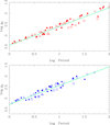 |
Fig. A.1. Relation between FWG and period for FU (top panel) and FO (bottom panel) models. The meaning of the symbols and colours is explained in Fig 1. The green lines refer to the best fits, Eqs. (A.1) and (A.2). |
Additional fits for the relations between FWG and period are given in Table A.2 and are illustrated in Fig. A.2. They show that when multiple gF values are available the scatter in the relation decreases. Assuming that the intrinsic scatter in the relation is 0.093 dex (Eq. (4)) a single determination has an estimated error of about 0.13 dex (dominated by the error on log g), while averaging six or more spectra leads to an error of about 0.09 dex.
As noted in the main text, and illustrated by comparing Fig. 4 and the top panel in Fig. A.2, a fair fraction of outliers are stars with Teff and log g taken from Genovali et al. (2014). Genovali et al. (2014) also present multiple observations for some stars, and XX Sgr and WZ Sgr are in common with the subsample of stars in L18 with five or more available spectra. A comparison shows that the difference in log gF is dominated by the difference in log g, that are of the order 0.5 dex. For some of the stars in the present sample the log gF (and log g) values are too low by 1 dex. As they seem to use the same methodology as L18 in deriving the stellar parameters, no simple explanation is offered to explain this discrepancy.
Fits of the type gF = a ⋅ log P + b.
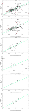 |
Fig. A.2. FWG vs period. The data from Genovali et al. (2014) is excluded in all plots. Different panels show different selections on the number of available gF values. From top to bottom: all, Nsp = 1, Nsp = 2, Nsp = 3−5, Nsp = 6−10, Nsp ≥ 11. The green lines refer to the best fits (see Table A.2). |
Table A.3 compiles the FWG and luminosity data for the entire sample. The full table is available at the CDS.
FWG data for the entire sample (first entries only).
All Tables
All Figures
|
Fig. 1. Top panel: FWGLR based on the pulsation models in Anderson et al. (2016). FU models are shown in red, FO models are shown in blue. For clarity FU (FO) models are plotted with an offset of +0.05 (−0.05) dex in Mbol. Symbols indicate the entry point of the IS, the lines connect it to the exit point of the IS. The first, second, and third crossing models are plotted as circles, squares, and triangles, respectively. Solar metallicity models are plotted with open symbols, models with Z = 0.006 with filled symbols. The black lines refer to Eqs. (1) and (2), the green line to the best fit (Eq. (3)). Bottom panel: relation between FWG and period for the same models. The period of the FO models was fundamentalised. The green line refers to the best fit, Eq. (4). |
| In the text | |
|
Fig. 2. FWG vs pulsation phase for four CCs. The typical error bar in each point is 0.15 dex in FWG, as indicated in the bottom plot. The lines are low-order harmonic fits to the data (see Col. 7 in Table 1). |
| In the text | |
|
Fig. 3. FWGLR based on the subsample with more than five spectra. FU mode pulsators are plotted as circles (filled circles for periods over 10 days), FO pulsators as open squares, the single second-overtone pulsator as open triangle. The black lines refer to Eqs. (1) and (2), the green line to Eq. (3). The blue line is a fit to the data points, excluding Y Oph (Eq. (5)). |
| In the text | |
|
Fig. 4. FWG vs fundamental pulsation period. Some outliers are named. The green line refers to the best fit, Eq. (6), which excludes the outliers and non-CCs indicated by a red cross. |
| In the text | |
|
Fig. 5. FWGLR, with some outliers named. The black lines refer to Eqs. (1) and (2), the green line to Eq. (3). The blue line refers to the best fit, Eq. (7), which excludes the outliers and non-CCs indicated by a red cross. Outliers located outside the plot window are SU Cru (log gF = 0.19, Mbol = −3.7), SY Nor (log gF = 2.4, Mbol = +3.3), and V382 Car (log gF = 1.8, Mbol = −8.6). |
| In the text | |
|
Fig. A.1. Relation between FWG and period for FU (top panel) and FO (bottom panel) models. The meaning of the symbols and colours is explained in Fig 1. The green lines refer to the best fits, Eqs. (A.1) and (A.2). |
| In the text | |
|
Fig. A.2. FWG vs period. The data from Genovali et al. (2014) is excluded in all plots. Different panels show different selections on the number of available gF values. From top to bottom: all, Nsp = 1, Nsp = 2, Nsp = 3−5, Nsp = 6−10, Nsp ≥ 11. The green lines refer to the best fits (see Table A.2). |
| In the text | |
Current usage metrics show cumulative count of Article Views (full-text article views including HTML views, PDF and ePub downloads, according to the available data) and Abstracts Views on Vision4Press platform.
Data correspond to usage on the plateform after 2015. The current usage metrics is available 48-96 hours after online publication and is updated daily on week days.
Initial download of the metrics may take a while.