| Issue |
A&A
Volume 640, August 2020
|
|
|---|---|---|
| Article Number | A5 | |
| Number of page(s) | 19 | |
| Section | Interstellar and circumstellar matter | |
| DOI | https://doi.org/10.1051/0004-6361/202037673 | |
| Published online | 28 July 2020 | |
Observed sizes of planet-forming disks trace viscous spreading
1
Leiden Observatory, Leiden University,
Niels Bohrweg 2,
2333 CA
Leiden, The Netherlands
e-mail: This email address is being protected from spambots. You need JavaScript enabled to view it.
2
Department of Astronomy, University of Michigan, 1085 S. University Ave,
Ann Arbor,
MI 48109, Michigan
3
Anton Pannekoek Institute for Astronomy, University of Amsterdam,
Science Park 904,
1090 GE
Amsterdam, The Netherlands
4
Max-Planck-institute für Extraterrestrische Physik,
Giessenbachstraße,
85748
Garching, Germany
Received:
5
February
2020
Accepted:
21
May
2020
Abstract
Context. The evolution of protoplanetary disks is dominated by the conservation of angular momentum, where the accretion of material onto the central star is fed by the viscous expansion of the outer disk or by disk winds extracting angular momentum without changing the disk size. Studying the time evolution of disk sizes therefore allows us to distinguish between viscous stresses or disk winds as the main mechanism of disk evolution. Observationally, estimates of the size of the gaseous disk are based on the extent of CO submillimeter rotational emission, which is also affected by the changing physical and chemical conditions in the disk during the evolution.
Aims. We study how the gas outer radius measured from the extent of the CO emission changes with time in a viscously expanding disk. We also investigate to what degree this observable gas outer radius is a suitable tracer of viscous spreading and whether current observations are consistent with viscous evolution.
Methods. For a set of observationally informed initial conditions we calculated the viscously evolved density structure at several disk ages and used the thermochemical code DALI to compute synthetic emission maps, from which we measured gas outer radii in a similar fashion as observations.
Results. The gas outer radii (RCO, 90%) measured from our models match the expectations of a viscously spreading disk: RCO, 90% increases with time and, for a given time, RCO, 90% is larger for a disk with a higher viscosity αvisc. However, in the extreme case in which the disk mass is low (Mdisk ≤ 10−4 M⊙) and αvisc is high (≥10−2), RCO, 90% instead decreases with time as a result of CO photodissociation in the outer disk. For most disk ages, RCO, 90% is up to ~12× larger than the characteristic size Rc of the disk, and RCO, 90%/Rc is largest for the most massive disk. As a result of this difference, a simple conversion of RCO, 90% to αvisc overestimates the true αvisc of the disk by up to an order of magnitude. Based on our models, we find that most observed gas outer radii in Lupus can be explained using viscously evolving disks that start out small (Rc(t = 0) ≃ 10 AU) and have a low viscosity (αvisc = 10−4−10−3).
Conclusions. Current observations are consistent with viscous evolution, but expanding the sample of observed gas disk sizes to star-forming regions, both younger and older, would better constrain the importance of viscous spreading during disk evolution.
Key words: protoplanetary disks / astrochemistry / radiative transfer / line: formation
© ESO 2020
1 Introduction
Planetary systems form and grow in protoplanetary disks. These disks provide the raw materials of gas and dust to form the increasingly diverse population of exoplanets and planetary systems that has been observed (see, e.g. Benz et al. 2014; Morton et al. 2016; Mordasini 2018). The formation of planets and the evolution of protoplanetary disks are closely related. While planets are forming, the disk is evolving around them, affecting the availability of material and providing constantly changing physical conditions around the planets. In a protoplanetary accretion disk, material is transported through the disk and accreted onto the star. We are still debating exactly which physical process dominates the angular momentum transport and drives the accretion flow, which is a crucial part of disk evolution.
It is commonly assumed that disks evolve under the influence of an effective viscosity, where viscous stresses and turbulence transport angular moment to the outer disk (see, e.g. Lynden-Bell & Pringle 1974; Shakura & Sunyaev 1973). As a consequence of the outward angular momentum transport, the bulk of the mass moves inward and is accreted onto the star. The physical processes that constitute this effective viscosity are still a matter of debate, magnetorotional instability being the most accepted mechanism (see, e.g. Balbus & Hawley 1991, 1998).
An alternative hypothesis is that angular momentum can be removed by disk winds rather than being transported through the disk (see, e.g. Turner et al. 2014 for a review). The presence of a vertical magnetic field in the disk can lead to the development of a magnetohydrodynamic (MHD) disk wind. These disk winds remove material from the surface of the disk and are thus able to provide some or all of the angular momentum removal required to fuel stellar accretion (see, e.g. Ferreira et al. 2006; Béthune et al. 2017; Zhu & Stone 2018). Direct observational evidence of such disk winds focuses on the inner part of the disk, but it is unclear whether winds dominate the transport of angular momentum and therefore how much winds affect the evolution of the disk (see, e.g. Pontoppidan et al. 2011; Bjerkeli et al. 2016; Tabone et al. 2017; de Valon et al. 2020).
Observationally these two scenarios make distinctly different predictions on how the sizes of protoplanetary disks evolve over time. In the viscous disk theory, conservation of angular momentum ensures that some parts of the disk move outward. As a result, disk sizes should grow with time. If instead disk sizes do not grow with time, disk winds are likely to drive disk evolution. To distinguish between viscous evolution and disk winds we need to define a disk size, which has to be measured or inferred from observed emission, and we must examine how it changes as a function of disk age.
With the advent of the Atacama Large Millimeter/sub-Millimeter Array (ALMA) it has become possible to perform large surveys of protoplanetary disks at high angular resolution. This has resulted in a large number of disks for which the extent of the millimeter continuum emission, the dust disk size, can be measured (see, e.g. Barenfeld et al. 2017; Cox et al. 2017; Tazzari et al. 2017; Ansdell et al. 2018; Cieza et al. 2018; Long et al. 2019). However, this continuum emission is predominantly produced bymillimeter-sized dust grains, which also undergo radial drift as a result of the drag force from the gas, an inward motion that complicates the picture. Moreover, radial drift and radially dependent grain growth lead to a dependence between the extent of the continuum emission and the wavelength of the observations; emission at longer wavelengths is more compact (see e.g. Tripathi et al. 2018).
Rosotti et al. (2019) used a modeling framework to study the combined effect of radial drift and viscous spreading on the observed dust disk sizes. They determined that to measure viscous spreading, the dust disk size has to be defined as a high fraction (≥95%) of the total continuum flux. To ensure that this dust disk size is well characterized, the dust continuum has to be resolved a signal-to-noise ratio (S/N). These authors show that existing surveys lack the sensitivity to detect viscous spreading.
To avoid having to disentangle the effects of radial drift from viscous spreading, we can instead measure a gas disk size from rotational line emission of molecules such as CO and CN, which are commonly observed in protoplanetary disks. An often used definition for the gas disk size is the radius that encloses 90% of the total CO J = 2−1 flux (RCO, 90%; see, e.g. Ansdell et al. 2018). This radius encloses most (>98%) of the disk mass and it has been shown that RCO, 90% is not affected by dust evolution (Trapman et al. 2019). The longer integration time required to detect this emission in the outer disk means that significant samples of measured gas disk sizes are only now becoming available (see, e.g. Barenfeld et al. 2017; Ansdell et al. 2018). Using a sample of measured gas disk sizes collated from literature, Najita & Bergin (2018) show tentative evidence that older Class II sources have larger gas disk sizes that the younger Class I sources; this is consistent with expectations for viscous spreading. It should be noted however that the gas disk sizes in their sample were measured using a variety of different tracers and observational definitions of the gas disk size.
When searching for viscous spreading using measured gas disk sizes it is important to keep in mind that these gas disk sizes are an observed quantity that are measured from molecular line emission. As the disk evolves, densities and temperatures change, affecting the column densities and excitation levels of the gas tracers used to measure the disk size. How well the observed gas outer radius traces viscous expansion has not been investigated in much detail.
Time-dependent chemistry also affects the gas tracers such as CO that we use to measure gas disk sizes. At lower densities CO, found in the outer disk and at a few scale heights above the midplane of the disk, is destroyed through photodissociation by UV radiation. Trapman et al. (2019) show that RCO, 90% traces the point in the outer disk where CO becomes photodissociated. Deeper in the disk, around the midplane where the temperature is low, CO freezes out onto dust grains. Once frozen out, CO can be converted into other molecules such as CO2, CH4 and CH3 OH (see, e.g. Bosman et al. 2018; Schwarz et al. 2018). These molecules have higher binding energies than CO and therefore stay frozen out at temperatures at which CO would normally desorb back into the gas phase. Through this process gas-phase CO can be more than an order of magnitude lower than the abundance of 10−4 with respectto molecular hydrogen, which is the expected abundance at which most of the volatile carbon is contained inCO (see, e.g. Lacy et al. 1994).
In this work, we set up disk models with observationally informed initial conditions, let the surface density evolve viscously, and use the thermochemical code DALI (Bruderer et al. 2012; Bruderer 2013) to study how the CO J = 2−1 intensity profiles, and the gas disk sizes derived from these profiles, change over time. We then compare these values with existing observationsto see if the observations are consistent with viscous evolution. This work is structured as follows: We introduce the setup and assumptions in our modeling in Sect. 2. In Sect. 3 we show how well observed gas outer radii trace viscous evolution both qualitatively and quantitatively. In Sect. 4 we compare our models to observations. We also study how chemical CO depletion through grain-surface chemistry affects our results. We discuss whether external photo-evaporation could explain the small observed gas disk sizes, compare our results to disk evolution driven by magnetic disks winds, and we discuss whether including episodic accretion would affect our results. We conclude in Sect. 5 that measured gas outer radii can be used to trace viscous spreading in disks.
2 Model setup
The gas disk size is commonly obtained from CO rotational line observations, for example, by measuring the radius that encloses 90% of the CO flux (e.g. Ansdell et al. 2018) or by fitting a power law to the observed visibilities (e.g. Barenfeld et al. 2017). In this work we used the radius that encloses 90% of the 12CO 2–1 flux (RCO, 90%) as the definition of the observed gas disk size. Trapman et al. (2019) show that RCO, 90% traces a fixed surface density in the outer disk, where CO becomes photodissociated. To see if RCO, 90% is a suitable tracer of viscous evolution, we are therefore interested in how the extent of the 12CO intensity changes over time in a viscously evolving disk.
Our approach for setting up our models is the following. First, we obtained a set of initial conditions that reproduce current observed stellar accretion rates, assuming that the disks feeding the stellar accretion have evolved viscously. Next we calculated the time evolution of the surface density. For each set of initial conditions, we analytically calculated the surface density profile (Σ(R, t)) at ten different disk ages. For each of these time steps we used the thermochemical code Dust and Lines (DALI; Bruderer et al. 2012; Bruderer 2013) to calculate the current temperature and chemical structure of the disk at that age and created synthetic emission maps of 12CO, from which we measured RCO, 90%.
2.1 Viscous evolution of the surface density
Accretion disks in which the disk structure is shaped by viscosity are often described using a α−disk formalism (Shakura & Sunyaev 1973), parameterizing the kinematic viscosity as ν = αcsH, where cs is the sound speed and H is the height above the midplane (Pringle 1981). For an α−disk, the self-similar solution for the surface density Σ is given by (Lynden-Bell & Pringle 1974; Hartmann et al. 1998)
![Mathematical equation: \begin{equation*}\Sigma_{\textrm{gas}}(R) = \frac{\left(2-\gamma\right){{M_{\textrm{disk}}}}(t)}{2\pi{{R_{\textrm{c}}}}(t)^2} \left( \frac{R}{{{R_{\textrm{c}}}}(t)} \right)^{-\gamma} \exp\left[ -\left(\frac{R}{{{R_{\textrm{c}}}}(t)}\right)^{2-\gamma}\right], \end{equation*}](/articles/aa/full_html/2020/08/aa37673-20/aa37673-20-eq1.png) (1)
(1)
where γ is set by assuming that the viscosityvaries radially as ν ∝ Rγ and Mdisk and Rc are the disk mass and the characteristic radius, respectively.
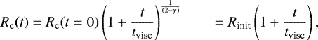
Following Hartmann et al. (1998), the time evolution of Mdisk and Rc is described by
![Mathematical equation: \begin{align*}&{{M_{\textrm{disk}}}}(t) = {{M_{\textrm{disk}}}}(t=0) \left(1 + \frac{t}{{{t_{\textrm{visc}}}}} \right)^{-\frac{1}{[2(2-\gamma)]}} = {{M_{\textrm{init}}}} \left(1 + \frac{t}{{{t_{\textrm{visc}}}}} \right)^{-\frac{1}{2}} \end{align*}](/articles/aa/full_html/2020/08/aa37673-20/aa37673-20-eq2.png) (2)
(2)
 (3)
(3)
where tvisc is the viscous timescale and we defined short hands for the initial disk mass Minit ≡ Mdisk(t = 0), the initial characteristic size Rinit ≡ Rc(t = 0). For the second step and the rest of this work, we assumed γ = 1 since for a typical temperature profile it corresponds to the case of a constant αvisc.
Combining Eqs. (1), (2), and (3) we obtain the time evolution of the surface density profile
![Mathematical equation: \begin{align*}\Sigma_{\textrm{gas}}(t,R) =&\, \frac{{{M_{\textrm{disk}}}}(t)}{2\pi{{R_{\textrm{c}}}}(t)^2} \left( \frac{R}{{{R_{\textrm{c}}}}(t)} \right)^{-1} \exp\left[ -\left(\frac{R}{{{R_{\textrm{c}}}}(t)}\right)\right]\\ =&\, \frac{{{M_{\textrm{init}}}}}{2\pi{{R_{\textrm{init}}}}^2} \left(1 + \frac{t}{{{t_{\textrm{visc}}}}} \right)^{-\frac{3}{2}} \left( \frac{R}{{{R_{\textrm{init}}}} \left(1 + \frac{t}{{{t_{\textrm{visc}}}}} \right)} \right)^{-1} \\ &\times \exp\left[ -\left(\frac{R}{{{R_{\textrm{init}}}} \left(1 + \frac{t}{{{t_{\textrm{visc}}}}} \right)}\right)\right]. \end{align*}](/articles/aa/full_html/2020/08/aa37673-20/aa37673-20-eq4.png)
2.2 Initial conditions of the models
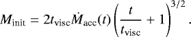
For a viscous disk the initial disk mass Minit is related to the stellar accretion rate through (Hartmann et al. 1998)
 (7)
(7)
Under the assumption that the disk evolved viscously, we calculated Minit given the stellar accretion rate measured at a time t and the viscous timescale of the disk. For various star-forming regions, for example, Lupus and Chamaeleon I, stellar accretion rates were determined from observations (see, e.g. Alcalá et al. 2014, 2017; Manara et al. 2017). A correlation was found between the stellar mass M* and the stellar accretion rate Ṁacc, best described by a broken power law. Based on Eq. (7) a disk around a more massive star therefore has a higher initial disk mass for the same viscous timescale.
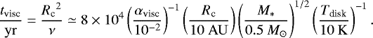
For our models we considered three stellar masses: 0.1, 0.32, and 1.0 M⊙. For each stellar mass, we used the observations, presented in Fig. 6 of Alcalá et al. (2017), to pick the average stellar accretion rate associated with that stellar mass. For each stellar accretion rate, we calculated the initial disk mass using Eq. (7) for three different viscous timescales. The viscous timescale is computed for three values of the dimensionless viscosity αvisc = 10−2, 10−3, 10−4, assuming a characteristic radius of 10 AU (which is the radius we employed; see below) and a disk temperature Tdisk of 20 K (see, e.g. e-quation 37 in Hartmann et al. 1998)
 (8)
(8)
The combination of three stellar accretion rates and three viscous timescales results in nine different disk models (see Table 1). Figure 1 shows how disk parameters such as Ṁacc, Rc, and Mdisk evolve with time for the models with M* = 0.1 M⊙. Similarly, Fig. A.1 shows how Mdisk evolves for the models with M* = 0.32 M⊙ and 1.0 M⊙. We note that the trends for Mdisk(t) are very similar, apart from starting at a higher initial Mdisk (~10−2 M⊙ for M* = 0.32 M⊙ and ~10−1 M⊙ for M* = 1.0 M⊙; cf. Table 1).
The initial size of disks is less well constrained, predominately because of a lack of high-resolution observations for younger Class 1 and 0 objects. Recently, Tobin et al. 2020 present the VANDAM II survey: 330 protostars in Orion observed at 0.87 millimeter with ALMA at a resolution of ~ 0.′′1 (~ 40 AU in diameter). By fitting a 2D Gaussian to their dust millimeter observations, the authors determined median dust disk radii of  AU and
  AU for theirClass 0 and Class 1 protostars, suggesting that the majority of disks are initially very compact. It should be noted that it is unclear whether the extent of the dust emission can be directly related to the gas disk size. However, there is also similar evidence from the gas that Class 1 and 0 objects are compact. As part of the CALYPSO large program, Maret et al. (2020) observed 16 Class 0 protostars and found that only two sources show Keplerian rotation at ~ 50 AU scales, suggesting that Keplerian disks larger than 50 AU, such as found for VLA 1623 (Murillo et al. 2013), are uncommon. We therefore adopted an initial disk size of Rinit = 10 AU for our models. In Sect. 4.2 we discuss the impact of this choice.
Initial conditions of our DALI models.
2.3 DALI models
Based on our nine sets of initial conditions, we calculated Mdisk and Rc at ten disk ages between 0.1 and 10 Myr using Eqs. (2) and (3) (see Fig. 1 for an example). From Mdisk(t) and Rc (t), we calculated Σgas(t) and used that as input for the thermochemical code DALI (Bruderer et al. 2012; Bruderer 2013). Based on a 2D physical disk structure, DALI calculates the thermal and chemical structure of the disk self-consistently. First, the dust temperature structure and the internal radiation field are computed using a 2D Monte Carlo method to solve the radiative transfer equation. In order to find a self-consistent solution, the code iteratively solves the time-dependent chemistry, calculates molecular and atomic excitation levels, and computes the gas temperature by balancing heating and cooling processes. The model can then be ray traced to construct synthetic emission maps. A more detailed description of the code is provided in Appendix A of Bruderer et al. (2012).
For the vertical structure of our models we assumed a Gaussian density distribution, with a radially increasing scale height of the form 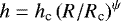 . In this equation, hc is the scale height at Rc and ψ is the flaring angle. The stellar spectrum used in our models is a black body with Teff = 4000 K. To this black body we added excess UV radiation, resulting from accretion, in the form of 10 000 K black body. For the luminosity of this component, we assume that the gravitational potential energy of the accreted mass is released with 100% efficiency (see, e.g. Kama et al. 2015). For the external UV radiation we assumed a standard interstellar radiation field of 1 G0 Habing 1968). These parameters are summarized in Table 2.
In our models we included the effects of dust settling by subdividing our grains into two populations. A population of small grains (0.005–1 μm) follows the gas density distribution both radially and vertically. A second population of large grains (1–103 μm), making up 90% of the dust by mass, follows the gas radially but has its scale height reduced by a factor χ = 0.2 with respect to the gas. We computed the dust opacities for both populations using a standard interstellar medium (ISM) dust composition following Weingartner & Draine (2001), with a Mathis-Rumpl-Nordsieck (MRN; Mathis et al. 1977) grain size distribution. We did not include any radial drift or radially varying grain growth in our DALI models (cf. Facchini et al. 2017). However, we note that Trapman et al. (2019) show that dust evolution does not affected measured gas outer radii.
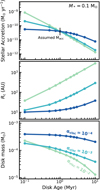 |
Fig. 1 Evolution of the disk parameters for the models with M* = 0.1 M⊙. The colors show different αvisc. For reference, the viscous timescales are 0.046, 0.46, and 4.6 Myr for αvisc = 10−2, 10−3, and 10−4, respectively. The evolution of the disk mass for the models with M* = 0.32 M⊙ and 1.0 M⊙ is shown Fig. A.1. For the model with αvisc = 10−2, Mdisk starts out at highermass compared to the model with αvisc = 10−3, but this model also loses mass at a faster rate. |
Fixed DALI parameters of the physical model.
3 Results
3.1 Time evolution of the 12CO emission profile
To first order, the evolution of 12CO intensity profile is determined by three time-dependent processes as follows:
- 1.
Viscous spreading moves material, including CO, to larger radii resulting in more extended CO emission.
- 2.
The disk mass decreases with time, lowering surface density, which in the outer disk allows CO to be more easily photodissociated. This removes CO from the outer disk and lowers the CO flux coming from these regions.
- 3.
Overlonger timescales, time-dependent chemistry results in CO being converted into CH4, CO2, and CH3OH. This is discussed separately in more detail in Sect. 4.3.
The combined effect of the first two processes on the 12CO emission profile can be seen in Fig. 2 for disks with a stellar mass of M* = 0.1 M⊙. Similar profiles for the remaining disks are shown in Fig. B.1
For a high αvisc of 0.01 the viscous timescale is short compared to the disk age and viscous evolution is happening fast. This is reflected in the 12CO emission, which spreads quickly (within 1 Myr) from ~200 to ~400 AU. After ~2 Myr the 12CO emission in the outer parts of the disk starts to decrease. At this point the total column densities in the outer disk are low enough that CO is removed through photodissociation. As a reference, by 2 Myr the disk mass of the models has dropped to Mdisk = 5 × 10⁻⁵ M⊙ and its characteristic size has increased to Rc = 400 AU (see Fig. 1).
For models with αvisc = 10−3, shown in the middle panel of Fig. 2, viscous spreading of the disk dominates the evolution of the 12CO emission profile. Compared to the αvisc = 10−2 models the column density in the outer disk never becomes low enough for CO to be efficiently photodissociated.
The models with αvisc = 10−4, presented in the right panel of Fig. 2, shows only small changes in the emission profile. For these models the viscous timescale is ~3.5 Myr, meaning that within the 10 Myr lifetime considered the surface density does not go through much viscous evolution.
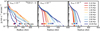 |
Fig. 2 Evolution of the 12CO 2–1 radial intensity profiles for models with M* = 0.1 M⊙. The colors indicate various disk ages between 0.1 and 10 Myr. The crosses at the bottom of each panel show the gas outer radius, defined as the radius that encloses 90% of the total 12CO 2–1 flux. |
3.2 Evolution of the observed gas outer radius
From the 12CO emission maps we can calculate the outer radius that would be obtained from observations. We define the observed gas outer radius, RCO, 90%, as the radius that encloses 90% of the total 12CO flux. A gas outer radius defined this way encloses most (>98%) of the disk mass and traces a fixed surface density in the outer disk (Trapman et al. 2019). We note that we do not include observational factors, such as noise, which affect the RCO, 90% that is measured. To accurately retrieve RCO, 90% from observations requires a peak S∕N > 10 on the moment zero map of the 12CO emission (cf. Trapman et al. 2019). The radii discussed in this work are measured from 12CO J =2−1 emission, but tests show that gas outer radii measured from 12CO J =3−2 are the same to within a few percent.
Figure 3 shows how the observed outer radius changes as a result of viscous evolution. The top panel shows RCO, 90% for models with M* = 0.1 M⊙. For αvisc = 10−2 the gas outer radius first increases until it starts to decrease at ~2 Myr. The decrease in RCO, 90% is due to decreasing column densities in the outer disk, allowing CO to be more easily photodissociated (for details, see Sect. 3.1). For αvisc = 10−3, RCO, 90% increases monotonically from ~70 to ~280 AU. The trend is similar forαvisc = 10−4 but RCO, 90% increases at a slower rate, ending up at RCO, 90% ~ 150 AU after 10 Myr.
For models with M* = 0.32 M⊙ and 1.0 M⊙, the initial and final disk masses are much higher compared to the models with M* = 0.1 M⊙. As a result, photodissociation does not have a significant effect on RCO, 90% and RCO, 90% does not significantly decrease with age. In addition, the disk sizes for these two groups of models are very similar. For αvisc = 10−2, RCO, 90% instead rapidly increases from ~180−250 AU at 0.1 Myr to 1500−1800 AU at 10 Myr. For αvisc = 10−3 the growth of RCO, 90% is less extreme in comparison, but observed disk sizes still reach 500−700 AU after 10 Myr. Owing to the long viscous timescales of 5−10 Myr for the models with αvisc = 10−4, RCO, 90% does not increase significantly (i.e., by less than a factor of ~2) over a disk lifetime of ~10 Myr.
For more embedded star-forming regions, the 12CO emission from the disk can be contaminated by the cloud, either by having 12CO emissionfrom the cloud mixed in with the emission from the disk or through cloud material along the line of sight absorbing the 12CO emission from the disk. This can prevent using 12CO to accurately measure disk sizes. We therefore also examined disk sizes measured using 90% of the 13CO 2–1 flux, which are shown in Fig. C.2. Apart from being a factor ~ 1.4−2 smaller than the 12CO outer radii, the 13CO outer radii evolve similarly as RCO, 90%. The 13CO outer radii are smaller than RCO, 90% because the less abundant 13CO is more easily removed in the outer parts of the disk through photodissociation. Our conclusions for RCO, 90% are therefore also applicable for gas disk sizes measured from 13CO emission. However, see Sect. 4.3 on how chemical depletion of CO through grain-surface chemistry affects this picture.
Overall we find that the observed outer radius increases with time and is larger for a disk with a higher αvisc. The exception to this rule are the models with low stellar mass (M* = 0.1 M⊙) and high viscosity (αvisc = 10−2). These highlight the caveat that if the disk mass becomes too low, CO becomes photodissociated in the outer disk and the observed outer radius decreases with time.
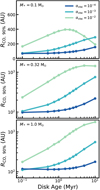 |
Fig. 3 Gas outer radius vs. disk age, defined as the radius that encloses 90% of the 12CO 2–1 flux. Top, middle, and bottom panels: models with various stellar masses (cf. Table 1). The colors correspond to the αvisc of the model. |
3.3 Gas outer radius traces viscous evolution
The previous section has shown that disks with higher αvisc, which evolveover a shorter viscous timescale, are overall larger at a given disk age. To quantify this, it is worthwhile to examine how well the observed gas outer radius RCO, 90% traces the characteristic size Rc of the disk.
Figure 4 shows the ratio RCO, 90%∕Rc as a function of disk age for the three sets of stellar masses. If RCO, 90% were only affected by viscous spreading it would grow at the same rate as the characteristic radius, RCO, 90% ∝ Rc, represented by a horizontal line in Fig. 4. Instead we see RCO, 90%∕Rc decreasing with disk age, indicating that the observed outer radius grows at a slower rate than the viscous spreading of the disk. The main cause for the slower growth rate of RCO, 90% is the decreasing disk mass over time because RCO, 90% traces a fixed surface density. As shown in Trapman et al. (2019), RCO, 90% coincides with the location in the outer disk, where CO is no longer able to effectively self-shield against photodissociation and is quickly removed from the gas. The CO column density threshold for CO to self-shield is NCO ≥ 1015 cm−2 (van Dishoeck & Black 1988). Thus, given that RCO, 90% traces a point of fixed column density, it scales with the total disk mass. As a result of angular momentum transport via viscous stresses, material is accreted onto the star, causing the total disk mass to decrease following Eq. (2) (see, e.g, Fig. 1), which limits the growth of RCO, 90%.
Figure 4 also shows that RCO, 90%∕Rc is larger for models with a lower αvisc; this difference becomes larger for older disks. This behavior can also be related to disk mass. As shown in Fig. 1 disk models with a lower αvisc have a higher disk mass. For the same Rc a higher disk mass, to first order, results in higher CO column densities in the outer disk. As a result CO is able to self-shield against photodissociation further out in the disk, increasing the difference between RCO, 90% and Rc.
In conclusion, we find that RCO, 90%∕Rc is between 0.1 and 12 and is mainly determined by the time evolution of the disk mass, which is set by the assumed viscosity. To infer Rc directly from RCO, 90% requires information on the total disk gas mass.
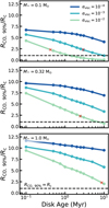 |
Fig. 4 Ratio of gas outer radius over characteristic radius vs. disk age. The black dashed line shows where RCO, 90% = Rc. Top, middle,and bottom panels: models with various stellar masses (cf. Table 1). The colors correspond to the αvisc of the model. The red crosses denote where RCO, 90%∕Rc = 2.3, that is, where RCO, 90% encloses 90% of the total disk mass (see Sect. 3.4). |
3.4 Possibility of measuring αvisc from observed RCO, 90%
A useful definition for an outer radius of a disk is that it encloses most of the mass in the disk. In this case, using a few simple assumptions, we can relate the outer radius directly to αvisc. If we assume that the viscous timescale at the outer radius of the disk, given by  , is approximately equal to the age of the disk, given by Ṁacc ≈ Mdisk∕tvisc, we can write αvisc as (see, e.g. Hartmann et al. 1998; Jones et al. 2012; Rosotti et al. 2017)
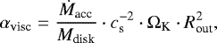 (9)
(9)
where Ṁacc is the stellar accretion rate, Mdisk is the total disk mass, cs is the sound speed, ΩK is the Keplerian orbital frequency, and Rout is the physical outer radius of the disk.
In absence of this physical outer radius, Ansdell et al. (2018) used the observed gas outer radius RCO, 90%, based on the 12CO 2–1 emission, to measure αvisc for 17 disks in Lupus finding a wide rangeof αvisc, spanning two orders of magnitude between 3 × 10⁻⁴ and 0.09.
For our models we have both RCO, 90%, measured from our models, and input αvisc, thus we can examine how well αvisc can be retrieved from the observed gasouter radius RCO, 90%. As we are mainly interested in the correlation between αvisc and RCO, 90%, we assume that M*, Ṁacc, and Mdisk are known, and cs is calculated assuming a disk temperature of 20 K, which is the same temperature used to calculate tvisc in Sect. 2.2.
Figure 5 shows αvisc measured using RCO, 90%, for our models and compares this value to the αvisc that was used as input for the models. For all disk models the measured αvisc decreases with age and, for most ages, we find αvisc(measured) > αvisc(input). Both of these observations can be traced back to which radius is used in Eq. (9) to calculate αvisc(measured). In the assumptions going into derivingEq. (9), Rout is defined asthe radius that encloses all (100%) of the mass of the disk. In our models in which the surface density follows a tapered power law the radius that encloses 100% of the mass is infinite, but we can instead take Rout as a radius that encloses a large, fixed fraction of the disk mass. For a tapered power law, this Rout is directly related to Rc. As an example, for a tapered power law where γ = 1, the radius that encloses 90% of the disk mass is 2.3 × Rc. For Rout = 2.3 × Rc in Eq. (9) we obtain approximately the same αvisc that was put into the model. Ideally we would therefore like RCO, 90% to also enclose a large, fixed fraction of the disk mass, or continuing our example, we would like RCO, 90% ≈ 2.3 × Rc, independent of disk age and mass. However, in Sect. 3.3 we show that RCO, 90%/Rc lies between 0.1 and 10 and decreases with disk age. Figure 4 shows that RCO, 90%∕Rc ≫ 2.3 for most disk ages, leading us to overestimate αvisc when measured from RCO, 90%. Taking the example discussed before, if we compare Figs. 5 and 4 we find that at disk ages where RCO, 90%∕Rc ≈ 2.3 our αvisc measured from RCO, 90% is within a factor of 2 of the input αvisc.
Summarizing we find that in most cases, RCO, 90%∕Rc ≫ 2.3 and we measure an αvisc much larger than the input αvisc, up to an order of magnitude higher, especially if the input αvisc is low. Given that at 1 Myr the measured αvisc is 5− 10× larger than the input αvisc, this implies that the αvisc determined by Ansdell et al. (2018) likely overestimates the true αvisc of the disks in Lupus by a factor 5–10.
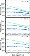 |
Fig. 5 Comparison between αvisc measured from RCO, 90% (solid line) and theinput αvisc (dashed line). The colors correspond to the input αvisc of the model. Top, middle, and bottom panels: models with different stellar masses (cf. Table 1). The red crosses denote where RCO, 90%∕Rc = 2.3 and RCO, 90% encloses 90% of Mdisk (cf. Sect. 3.4 and Fig. 4). The red crosses denote where RCO, 90%∕Rc = 2.3, that is, where RCO, 90% encloses 90% of the total disk mass (see Sect. 3.4). |
4 Discussion
4.1 Comparing to observations
Gas disk sizes have now been measured consistently for a significant number of disks. In contrast with Najita & Bergin (2018), in this paper we chose to select homogeneous samples (in terms of analysis and tracer). These samples are Ansdell et al. (2018) and Barenfeld et al. (2017), who measured RCO, 90% for 22 sources in Lupus and 7 sources in Upper Sco. Between them, these disks span between 0.5 and 11 Myr in disk ages. In Fig. 6 we compare our models to these observations, where sources with M* ≤ 0.66 M⊙ are compared to models with M* = 0.32 M⊙ and those with M* > 0.66 M⊙ are compared to models with M* = 1.0 M⊙. Ansdell et al. (2018) define the gas outer radius as the radius that encloses 90% of the 12CO 2–1 emission, so we take their values directly. For the disks in Upper Sco we calculate RCO, 90% from their fit to the observed 12CO intensity (cf. Barenfeld et al. 2017). Stellar ages and masses were determined by comparing pre-main-sequence evolutionary models to X-shooter observations of these sources (Alcalá et al. 2014, 2017). Lacking such observations for Upper Sco, we instead use the 5-11 Myr stellar age of Upper Sco (see, e.g. Preibisch et al. 2002; Pecaut et al. 2012) for all sources in this region. The observations are summarized in Table D.1.
As shown in Fig. 6, most of the Lupus observations lie between the models with αvisc = 10−3 and αvisc = 10−4. Most of thedisks can therefore been explained as viscously spreading disks with αvisc = 10−4−10−3 that start out small (Rinit = 10 AU). Only two sources with M* = 1.0 M⊙, IM Lup and Sz 98 (also known as HK Lup),require a larger αvisc ≃ 10−2 to explain the observed gas disk size given their age.
It is interesting to note that Lodato et al. (2017) reached a similar conclusion using a completely different method. They show that a simple viscous model can reproduce the observed relation between stellar mass accretion and disk mass in Lupus (see Manara et al. 2016). To match both the average disk lifetime and the observed scatter in the Ṁacc–Mdisk relation, disk ages in Lupus have to be comparable to the viscous timescale, on the order of ~ 1 Myr (see also Jones et al. 2012; Rosotti et al. 2017). This viscous timescale is comparable to our models with αvisc = 10−3 (cf. Table 1).
As we made no attempt to match our models to individual observations, it is worthwhile to discuss if it is possible to explain the large disks in our sample, such as IM Lup and Sz 98, by other means than a large αvisc. A quick comparison with Table 1 shows that increasing the disk mass does not help to explain their large RCO, 90%. Our models with M* = 1.0 M⊙ and αvisc = 10−3−10−4 differ by an order of magnitude in initial disk mass, but at 0.75 Myr they differ by less than 5% in terms of RCO, 90%. Another possibility would be increasing the initial disk size Rc(t = 0), which we discuss in Sect. 4.2.
Interestingly, five of the seven Upper Sco disks have gas outer radii that lie well below our models with αvisc = 10−4, indicating that their small RCO, 90% cannot be explained by our models, even when taking into account the uncertainty on their age. As the viscous timescale for our models with αvisc = 10−4 is already ~ 10 Myr, decreasing αvisc does not allow us to reproduce the observed RCO, 90%. At face value, these small disk sizes would thus seem to rule out that these disks have evolved viscously. We note, however, that there are processes which, in combination with viscous evolution, could explain these small disk sizes. The first would consist in reducing the CO content of these disks; we discuss this option in Sect. 4.3. Given that the disks in Upper Sco are highly irradiated as members of the Sco-Cen OB association (see e.g. Sect. 4.4 and Appendix E), another option is that external photo-evaporation is the culprit for their small disk sizes, but we cannot rule out a contribution of MHD disks winds to their evolution.
We have shown that the current observations in Lupus are consistent with viscous disk evolution with a low effective viscosity of αvisc = 10−3−10−4 (viscous timescales of 1−10 Myr). However, the current available data do not provide sufficient evidence for viscous spreading, which is the proof that viscosity is driving disk evolution. We stress that this is mostly because most of the available data come from the same star-formingregion (Lupus), and therefore most of the disks are concentrated around a disk age range from 1 to 3 Myr. Only a few disks lie outside this range. The inclusion of the Upper Sco disks would help constrain the importance of viscous spreading, but we already commented in the previous paragraph about the caveats with this region. Thus, we conclude that the current sample of radii is insufficient to confirm or reject the hypothesis that disks are viscously spreading. To overcome this problem, future observational campaigns should focus on expanding the observational sample of well-measured disk CO radii in other star-forming regions with a different age than Lupus.
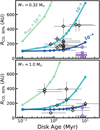 |
Fig. 6 Gas outer radii of our models (RCO, 90%) compared to observations. The colors correspond to the αvisc of the model. The black open diamonds show observed gas outer radii in Lupus (Ansdell et al. 2018) and the purple open squares denote observed gas outer radii in Upper Sco (Barenfeld et al. 2017). The Upper Sco outer radii shown are 90% outer radii, calculated from their fit to the observed 12CO intensity. The top and bottom panels split models and observations based on stellar mass. The sources with M* ≤ 0.66 M⊙ are compared to models with M* = 0.32 M⊙; those with M* > 0.66 M⊙ are compared to models with M* = 1.0 M⊙. Only panels for M* = 0.32 and 1.0 M⊙ are shown because the sample of observations considered in this work does not contain any objects with M* ~ 0.1 M⊙. |
4.2 Larger initial disk sizes
In our analysis we assumed that disks start out small, with Rinit = 10 AU, as motivated by recent ALMA observations of disks around young Class 0 and 1 protostars (Maury et al. 2019; Maret et al. 2020; Tobin et al. 2020). However, these observations also show a spread in disk size for these young objects. Increasing the initial disk size would potentially also allow us to explain the larger disks, for example, IM Lup and Sz 98 (see van Terwisga et al. 2018), which have a lower αvisc.
Figure 7 presents RCO, 90% measured from three sets of models with M* = 1.0 M⊙ (see Sect. 2.2), but with an increased Rinit = [30, 50, 100] AU. Since our models with Rinit = 10 AU and αvisc = 10−2 already have RCO, 90% much larger than what is observed, we only run these new models for αvisc = [10−3, 10−4]. These models have much larger gas disk sizes than models with Rinit = 10 AU; RCO, 90% is at least three times larger (RCO, 90% ≥ 300 AU). As such, they show that the large disks in the sample (RCO, 90%, obs. ≥ 300 AU) can also be explained with a larger initial size (Rinit = 30) and a low viscous alpha (αvisc = 10−4). Extrapolating our results beyond 1 Myr and to models with M* = 0.32 M⊙ there are six examples of such large disks in Lupus that can be explained with Rinit ≈ 30 AU (cf. Fig. 6). In particular these models show that the observed gas disk sizes of IM Lup and Sz 98 can be explained by either a high viscous alpha (Rinit = 10 AU, αvisc = 10−2) or a larger initial disk size (Rinit ≃ 30−50 AU, αvisc = 10−3−10−4). Given the similarities in terms of RCO, 90% between models with M* = 1.0 M⊙ and M* = 0.32 M⊙ seen in Fig. 3, we expect that increasing Rinit from 10 to 30 AU for models with M* = 0.32 M⊙ would similarly increase their RCO, 90% by a factor of at least 3.
However, our models show that disks with Rinit = 30 AU start out at RCO, 90% ~ 300 AU, which is already much larger than most observed RCO, 90% in Lupus (Ansdell et al. 2018). This indicates that, even if a larger Rinit can provide an explanation for these six disks, the bulk of the disks in Lupus cannot have had a large Rinit and they must have started out small (Rinit ≃ 10 AU). This could be in line with the observations of Tobin et al. (2020), although their measured dust radii should be multiplied by a factor of typically two to three to get the gas radii due to optical depth effects (Trapman et al. 2019).
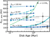 |
Fig. 7 Zoom in of the bottom panel of Fig. 6, showing gas outer radii of our models (RCO, 90%) compared to observations. Also added are models with M* = 1.0 M⊙ (see Sect. 2.2) but with Rinit = 30, 50, and 100 AU denoted with dotted, dashed-dotted, and dashed lines, respectively. The colors indicated different values for αvisc. The new models were only run for αvisc = [10−3, 10−4]. |
4.3 Effect of chemical CO depletion on measurements of viscous spreading
Over the recent years it has become apparent in observations that protoplanetary disks are underabundant in gaseous CO with respect to the expected abundance of CO∕H2 = 10−4 (see, e.g. Favre et al. 2013; Du et al. 2015; Kama et al. 2016; Bergin et al. 2016; Trapman et al. 2017). Several authors have shown that grain-surface chemistry is able to lower the CO abundance in disks, by converting CO into CO2 and CH3OH on the grains on a timescale of several million years (see, e.g. Bosman et al. 2018; Schwarz et al. 2018). In this work we refer to this process as chemical depletion of CO to distinguish it from simple freeze out of CO, which is included in our models presented in Sect. 3. As the chemical depletion of CO operates on similar timescales as viscous evolution, it can have a large impact on the use of 12CO as a probe for viscous evolution. We implement an approximate description for grain surface chemistry and examine its effects on observed gas outer radii. A more detailed description can be found in Appendix F.
Figure 8 shows 12CO 2–1 and 13CO –1 intensity profiles, with and without including chemical CO depletion, for two models at different disk ages. The 12CO 2–1 radial intensity profile remains unchanged until 10 Myr, at which point the intensities start to drop between ~ 100 and ~ 300 AU, seemingly carving a small “dip” in the intensity profile. With our current definition of the outer radius at 90% of the total flux, this dip lies within RCO, 90%. The decreasing intensity due to chemical COdepletion causes RCO, 90% to move outward, although the change is small (≤2%). The chemical depletion of CO does not affect the CO abundance beyond 300 AU (see, e.g. Fig. F.1), so the 12CO 2–1 flux originating from > 300 AU now makes up a larger fraction of the total 12CO flux when comparing models with and without chemical CO depletion. It should therefore be noted that if we were to change our definition of the gas outer radius such that it lies within the “dip”, for example, by defining RCO, X% using a lower percentage of the total flux, RCO, X% would decrease if we include chemical depletion of CO.
In contrast, the 13CO 2–1 intensity profile, shown in the right panels of Fig. 8, is significantly affected by chemical CO depletion at 10 Myr. Between ~100 and ~300 AU the 13CO intensity profile has dropped by more than an order of magnitude. Again, as an consequence of the infinite S/N of our synthetic emission maps, the decrease in the intensity profile has moved the radius enclosing 90% of flux outward. For real observations, in which the S/N is limited, chemical depletion of CO instead significantly decreases the observed outer radius if measured from 13CO emission. Figure 8 shows that gas disk sizes measured from 13CO can only be interpreted correctly if CO depletion is taken into account in the analysis. The figure also highlights the importance of high S/N observations when measuring gas disk sizes from 13CO emission. Given the lack of a significant sample of observed 13CO outer radii, we do not investigate this aspect in this paper further. We note however that once such a sample becomes available, an analysis quantifying the effect of chemical depletion on 13CO outer radii will become possible.
As shown in Fig. F.1, there exists a vertical gradient in CO abundances. Vertical mixing, not included in our models, would move CO rich gas from the 12CO emission layer toward the midplane and exchange it with CO-poor gas. If we were to include vertical mixing, the CO abundance in the 12CO emitting layer would decrease and thus the effect of CO depletion on RCO, 90% measured from 12CO would increase. The effect would be similar to what is seen for 13CO, indicating that in this case chemical CO depletion could also affect gas disk sizes measured from 12CO emission and should thus be taken into account in the analysis (see, e.g. Krijt et al. 2018; Krijt et al., in prep.)
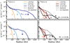 |
Fig. 8 Effect of chemical CO depletion through grain-surface chemistry on the 12CO 2–1 intensityprofile (left panels) and 13CO 2–1 intensity profile (right panels) after 1 Myr (orange), 3 Myr (light blue/dark red), and 10 Myr (blue/black). Top and bottom rows:models with M* = 0.32 M⊙ and M* = 1.0 M⊙, respectively. The profile without chemical CO depletion is shown as a dashed line. The gas outer radii (RCO, 90%) are shown as a cross at arbitrary height below the profile. After 1 Myr the chemical CO depletion is not significant enough to change the intensity profile and RCO, 90%. After 10 Myr chemical CO depletion causes RCO, 90% to increase (for details, see Sect. 4.3). Figures C.1 and G.1 give a full overview of the 13CO 2–1 intensity profile of the models without and with chemical CO depletion. |
4.4 Caveats
Photo-evaporation
In this paper we considered a disk evolving purely under the influence of viscosity. In reality, it is well known that pure viscous evolution cannot account for the observed timescale of a few million years on which disks disperse (see Alexander et al. 2014 for a review). Internal photo-evaporation is commonly invoked as a mass-loss mechanism to solve this problem. Because photo-evaporation preferentially removes mass from the inner disk (a few AUs), it is unlikely to change our conclusions. We note however that some photo-evaporation models (Gorti & Hollenbach 2009) have an additional peak in the mass-loss profile at a scale of 100–200 AU, which might influence our results.
Another potential concern is the effect of external photo-evaporation, that is, mass loss induced by the high-energy radiation emitted by nearby massive stars. In this case, the mass-loss preferentially affects the outer part of the disk (Adams et al. 2004) and might therefore have an influence on the evolution of the outer disk radius, likely moving RCO, 90% inward. The importance of this effect is region-dependent. A region like Lupus is exposed to relatively low levels of irradiation (see the appendix in Cleeves et al. 2016) and neglecting external photo-evaporation is probably safe in this case, although the effect can still be important for the largest disks (Haworth et al. 2017). For other regions, such as Upper Sco, the impact of external photo-evaporation is potentially more severe since the region is part of the nearest OB association, Sco-Cen (Preibisch & Mamajek 2008). According to the catalog of de Zeeuw et al. (1999), the earliest spectral type in the region is B0 and there are 49 B stars in the complex, suggesting that the level of irradiation can be significantly higher than in Lupus. A simple calculation, outlined in Appendix E, suggeststhat the disks in Upper Sco are currently subjected to a far-ultraviolet (FUV) radiation field of 10− 300 G0. For these levels of external UV radiation the mass-loss rate due to external photo-evaporation at radii of ~ 100 AU is ~ 10−9−10−8 M⊙yr−1, which is of the same order of magnitude as the accretion rate (see, e.g. Facchini et al. 2016; Haworth et al. 2017, 2018). Given the age of the region, stars with even earlier spectral types might have been present but are now evolved, as shown by the red supergiant Antares, implying that in the past the region was subject to a more intense UV flux than it is at the present.
Magnetic disk winds versus viscous evolution
In Sect. 4.1 we have shown that the observations in Lupus match with our viscously spreading disk models with αvisc = 10−3−10−4. However, we cannot exclude an alternative interpretation in which the observed RCO, 90% and stellar ages of individual disks could be reproduced by models in which disk evolution is driven by disk winds with a suitable choice of parameters. Figure 6 should therefore not be considered a confirmation of viscous evolution in disks. To properly distinguish between whether viscous stresses or disk winds are the dominant driver of disk evolution requires an observation of viscous spreading (or lack thereof), that is, that the average disk grows in size over time. Additionally, a search for disk winds in the objects discussed in this paper could allow us to quantitatively compare how much specific angular momentum is extracted by disk winds and how much is transported outward by viscous stresses.
Episodic accretion
In this work we have assumed a simple prescription of viscous evolution, where viscosity in the disk is described by a single parameter αvisc, which is kept constant in time and does not vary with radius. In reality this is likely to be a too simplistic view. For example, there is an increasing amount of evidence that stellar accretion is episodic rather than the smooth process assumed in this work (see, e.g. Audard et al. 2014 for a review). It is likely however that episodic accretion is most important in the early phases when the star is being assembled, and probably less in the later Class II phase (see, e.g. Costigan et al. 2014; Venuti et al. 2015).
If accretion were also episodic in the Class II phase, the growth of the disk size is likely also to be episodic, rather than the smooth curves shown in this work. However, to reproduce the average observed accretion rate, the episodic accretion rate averaged over time should still match the smooth accretion rate assumed in this work. Observationally, we cannot perform an average over time since the variational timescales, if any exists in the class II phase, are longer than what can be practically measured; observational studies find that accretion is modulated on the rotational period of the star (Costigan et al. 2014; Venuti et al. 2015), but that there is no variation on longer timescales. However, averaging over a sample of similar sources is mathematically equivalent to the average over time since they are at different stages of their duty cycle. Overall, the values for αvisc discussed in this work thus should be intended as some kind of average over its variations in space and time.
Related to the topic of episodic accretion is the connection, at an early age, between the disk and its surrounding envelope. Material is accreted from this envelope onto the disk; current evidence indicates that this could still be ongoing into the Class I phase (see, e.g. Yen et al. 2019). While this might affect our results at early ages (0.1–0.5 Myr) it is unlikely to change our results at a later age when accretion from the envelope onto the disk has stopped, and this would be equivalent to changing the initial disk mass or the initial disk size.
5 Conclusions
In this work we used the thermochemical code DALI to examine how the extent of the CO emission changes with time in a viscously expanding disk model and investigate how well this observed measure of the gas disk size can be used to trace viscous evolution. We summarize our conclusions as follows:
-
Qualitatively the gas outer radius RCO, 90% measured from the 12CO emission of our models matches the signatures of a viscously spreading disk: RCO, 90% increases with time and does so at a faster rate if the disk has a higher viscous αvisc (i.e., when it evolves on a shorter viscous timescale).
-
For disks with high viscosity (αvisc ≥ 10−2), the combination of a rapidly expanding disk with a low initial disk mass (Mdisk ≤ 2 × 10⁻⁴ M⊙) can result in the observed outer radius decreasing with time because CO is photodissociated in the outer disk.
-
For most of our models, RCO, 90% is up to ~12× larger than the characteristic size Rc of the disk, with the difference being larger for more massive disks. As a result, measuring αvisc directly from observed RCO, 90% overestimates the true αvisc of the disk by up to an order of magnitude.
-
Current measurements of gas outer radii in Lupus can be explained using viscously expanding disks with αvisc = 10−4−103 that start out small (Rinit = 10 AU). The exceptions are IM Lup (Sz 82) and HK Lup (Sz 98), which require either a higher αvisc ≈ 10−2 or a larger initial disk size of Rinit = 30−50 AU to explain their large gas disk size.
-
Chemical depletion of CO through grain-surface chemistry has only minimal impact on the RCO, 90% if measured from 12CO emission, but can significantly reduce RCO, 90% at 5–10 Myr if measured from more optically thin tracers such as 13CO.
We have shown that measured gas outer radii can be used to trace viscous spreading of disks and that models that fully simulate the observations play an essential role in linking the measured gas outer radius to the underlying physical size of the disk. Our analysis shows that current observations in Lupus are consistent with most disks starting out small and evolving viscously with low αvisc. However, most sources lie within an age range between 1Myr and 3 Myr, which is too narrow to confirm that disk evolution is only driven by viscosity. We therefore cannot rule out that disk winds are contributing to the evolution of the disk. Future observationsshould focus on expanding the available sample of observe gas disk sizes to other star-forming regions, both younger and older than Lupus, to conclusively show whether disks are viscous spreading and confirm whether viscosity is the dominant physics driving disk evolution.
Acknowledgements
We thank the referee for a very careful reading of the manuscript. L.T. and M.R.H. are supported by NWO grant 614.001.352. G.R. acknowledges support from the Netherlands Organisation for Scientific Research (NWO, program number 016.Veni.192.233). A.D.B. acknowledges support from NSF Grant#1907653. Astrochemistry in Leiden is supported by the Netherlands Research School for Astronomy(NOVA). All figures were generated with the PYTHON-based package MATPLOTLIB (Hunter 2007). This research made use of Astropy (http://www.astropy.org), a community-developed core Python package for Astronomy (Astropy Collaboration 2013, 2018).
Appendix A Disk mass evolution
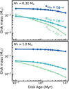 |
Fig. A.1 Evolution of the disk mass for the models with M* = 0.32 M⊙ and 1.0 M⊙. Evolution of the disk mass for models with M* = 0.1 M⊙ is shown in Fig. 1. The colors show models with different αvisc. The order of magnitude difference between the M* = 0.32 M⊙ models (top panel) and M* = 1.0 M⊙ models (bottom panel) are shown. |
Appendix B 12CO radial intensity profiles
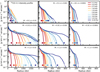 |
Fig. B.1 Time evolution of the 12CO intensity profiles for our grid of models. Rows: models with equal stellar mass. Columns: models with equal αvisc. The colors, going from red to blue, show the different time steps. For each model, the radius enclosing 90% of the total flux is denoted by a cross. A low stellar mass corresponds to a low stellar accretion rate, using the observational relation shown in Fig. 6 in Alcalá et al. (2017). Also owing to the setup, a low αvisc corresponds to a high viscous time (tvisc) and a high initial mass (Minit). |
Appendix C Outer radii based 13CO emission
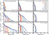 |
Fig. C.1 Time evolution of the 13CO intensity profiles for our grid of models. Rows: models with equal stellar mass; columns: models with equal αvisc. The colors, going from red to blue, show the different time steps. For each model, the radius enclosing 90% of the total flux is denoted by a cross. A low stellar mass corresponds to a low stellar accretion rate, usingthe observational relation shown in Fig. 6 in Alcalá et al. (2017). Also owing the setup, a low αvisc corresponds to a high viscous time (tvisc) and a high initial mass (Minit). |
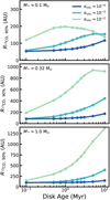 |
Fig. C.2 Disk ages vs. gas outer radii (RCO, 90%), measured from 13CO 2–1 emission. Top, middle, and bottom panels: models with different stellar masses. The colors indicate the αvisc of the model. |
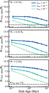 |
Fig. C.3 Ratio of gas outer radius ( |


Appendix D Observed sample
Observations in Lupus and Upper Sco.
Appendix E Local UV radiation field in Upper Sco
Because they belong to the nearest OB association, the disks in Upper Sco are likely to be subjected to high levels of irradiation. In this appendix, we quantify this these irradiation levels using the locations of known B stars (de Zeeuw et al. 1999) and the disks in Upper Sco (see Fig. E.1).
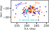 |
Fig. E.1 Spatial distribution of the disks in Upper Sco (colored circles) and the 49 B stars (blue crosses). The light blue cross denotes the location of V* del Sco, a B0.3V star that contributes significantly to the UV radiation in the region. |
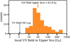 |
Fig. E.2 Histogram of the local UV radiation field for disks in Upper Sco. Radiation fields were calculated for each disk using Eq. (E.1). The orange arrow denotes the median UV radiation field. For comparison, the black arrow shows the external UV radiation field of IM Lup (Cleeves et al. 2016). |
Barenfeld et al. (2016) present ALMA observations of a sample of 106 stars in Upper Sco between spectral types of M5 and G2, selected based on the excess infrared emission observed by Spitzer or WISE (Carpenter et al. 2006; Luhman & Mamajek 2012). Parallaxes for 96 of these 106 stars were measured with Gaia as part of its DR2 data release (Gaia Collaboration 2018). We use these parallaxes to calculate the distance to each of the stars. For the 10 stars in which no parallax is available, we instead assume the distance to be 143 pc, which is the median distance to Upper Sco based on the DR2 data (see, e.g. Bailer-Jones et al. 2018; Wright & Mamajek 2018; Damiani et al. 2019).
In close proximity to these disk-hosting stars there are 49 stars with spectral type B1 and the region hosts one B0.3V star (V* del Sco; see, e.g. de Zeeuw et al. 1999; de Bruijne 1999). With the exception of the B0 star, these stars are also part of Gaia DR2, allowing us to determine distances to these stars based on their parallaxes. The B0 star, V* del Sco, is too bright to be part of Gaia DR2. For this star we use a distance of 224 ± 24 pc, which was calculated by Megier et al. (2009) based on interstellar Ca II lines. Combining these positions and distances, we can now calculate, for each disk-hosting star, the relative distances between it and each of the B stars.
To calculate the local FUV radiation field, we take the following approach: We collect the spectral types of the 49 B stars from the catalog of de Bruijne (1999) and use them to compute their effective temperatures following Hillenbrand & White (2004). Based on these effective temperature we fit stellar masses using the stellar models from Schaller et al. (1992). Using the stellar masses we calculate the UV luminosity LUV, B star produced by each star based on the relation presented in Buser & Kurucz (1992). Finally, for each disk in the sample from Barenfeld et al. (2016), we calculate the local UV radiation (FUV, disk) by adding up the relative contributions of each of the nearby B stars, that is,
 (E.1)
(E.1)
where |xdisk − xB star| denotes the relative distance between the disk and the B star.
Figure E.2 shows a histogram of the local UV radiation FUV, disk for the disks in Upper Sco. Levels range from ~8 G0 to ~7 × 10³ G0, with a median FUV, disk = 42.9 G0, confirming that these disks are subjected to high levels of external UV radiation. Even the lowest FUV, disk (~ 8 G0) is several times higher than the external UV field in Lupus (~3 G0; Cleeves et al. 2016).
Owing to the age of Upper Sco (5–11; see Preibisch et al. 2002; Pecaut et al. 2012), stars with spectral types earlier than B0.3, with lifetimes of a few up to 10 Myr might have been present in the region but are now evolved. It is therefore likely that external UV radiation in Upper Sco was higher in the past, suggesting that the FUV, disk calculated in this work is a lower limit of what the disks in Upper Sco experienced during their lifetime.
Appendix F Implementing CO chemical depletion through grain-surface chemistry
Based on the results from Bosman et al. (2018), we developed an approximated description for CO grain surface chemistry. The description only traces the main carbon carriers, that is, CO, CH3OH, CO2, and CH4. Briefly, the approximation splits reactions into two groups, fast and slow reactions, and assumes that fast reactions can be calculated by equilibrium chemistry and that only the slow reactions need to be integrated explicitly. A more detailed description is provided in the appendix of Krijt et al., in prep. The approximation breaks down in the upper regions of the disk, where photodissociation of CO by UV photons becomes important. In these regions the chemistry included in DALI provides more accurate CO abundances. We therefore split our disk models into two regions based on the outward CO column:
NCO < 1016 cm−2: the outward CO column is too low for CO to self-shield against photodissociation. As a result the CO chemistry is accurately described by the photochemistry included in DALI and we therefore do not recompute the CO abundances.
NCO ≥ 1016 cm−2: deeper in the disk CO is able to self-shield against photodissociation. Grain-surface chemistry is able to convert CO into other species, thus lowering the gas-phase abundance of CO. For this region we recompute the CO abundances using the approximate grain-surface chemistry from Krijt et al., in prep.
Figure F.1 presents the CO abundance structure with and without including CO depletion through grain-surface chemistry. At 1 Myr, shown in left panels, the inclusion of grain-surface chemistry has little impact on the CO abundance. However, at 10 Myr CO has become significantly depleted (X[CO] ≤ 10−8) around the midplane of the disk. We obtain the same conclusion as Bosman et al. (2018), namely that CO depletion only becomes significantly long timescales. Among our models we are only starting to see its effects after ≥ 5 Myr, indicating this process is most important for older star-forming regions such as Upper Sco.
 |
Fig. F.1 Effect of chemical depletion of CO through grain-surface chemistry on the CO abundanceafter 1 Myr (left panels) and 10 Myr (right panels). The example model shown has M* = 0.32 M⊙ and αvisc = 10−3. The colors show the CO abundance with respect to H2, where white indicates CO/H2 ≤ 10−8. The black contours show the 12CO 2–1 emittingregion, enclosing 25 and 75% of the total 12CO flux. Similarly, the red contours show the 13CO 2–1 emitting region. |
Figure F.1 also shows the emitting layers of 12CO 2–1 and 13CO 2–1. The chemical conversion of CO into other species predominantly takes place around the midplane, while the CO emittinglayer is higher up in the disk. For 12CO 2–1 the emitting layer lies predominantly in the region of the disk, where the CO abundances are set by photodissociation and not grain-surface chemistry, and are therefore only slightly affected by CO chemistry after 10 Myr. The emitting layer of 13CO 2–1 lies deeper in the disk and is therefore significantly affected by the conversion of CO.
Appendix G Effect of CO depletion on the 13CO emission
 |
Fig. G.1 Time evolution of the 13CO intensityprofiles for our grid of models, after including the effects of chemical depletion of CO through grain surface chemistry (see Sects. 4.3 and F). Rows: models with equal stellar mass, columns: models with equal αvisc. The colors, going from red to blue, show the different time steps. For each model, the radius enclosing 90% of the total flux is indicated by a cross. A low stellar mass corresponds to a low stellar accretion rate, using the observational relation shown in Fig. 6 in Alcalá et al. (2017). Also owing to the setup, a low αvisc corresponds to a high viscous time (tvisc) and a high initial mass (Minit). |
References
- Adams, F. C., Hollenbach, D., Laughlin, G., & Gorti, U. 2004, ApJ, 611, 360 [NASA ADS] [CrossRef] [Google Scholar]
- Alcalá, J., Natta, A., Manara, C., et al. 2014, A&A, 561, A2 [NASA ADS] [CrossRef] [EDP Sciences] [Google Scholar]
- Alcalá, J., Manara, C., Natta, A., et al. 2017, A&A, 600, A20 [NASA ADS] [CrossRef] [EDP Sciences] [Google Scholar]
- Alexander, R., Pascucci, I., Andrews, S., Armitage, P., & Cieza, L. 2014, in Protostars and Planets VI, eds. H. Beuther, R. S. Klessen, C. P. Dullemond, & T. Henning (Tucson: University of Arizona Press), 475 [Google Scholar]
- Andrews, S. M., Terrell, M., Tripathi, A., et al. 2018, ApJ, 865, 157 [NASA ADS] [CrossRef] [Google Scholar]
- Ansdell, M., Williams, J. P., Trapman, L., et al. 2018, ApJ, 859, 21 [NASA ADS] [CrossRef] [Google Scholar]
- Astropy Collaboration (Robitaille, T. P., et al.) 2013, A&A, 558, A33 [NASA ADS] [CrossRef] [EDP Sciences] [Google Scholar]
- Astropy Collaboration (Price-Whelan, A. M., et al.) 2018, AJ, 156, 123 [Google Scholar]
- Audard, M., Ábrahám, P., Dunham, M. M., et al. 2014, in Protostars and Planets VI, eds. H. Beuther, R. S. Klessen, C. P. Dullemond, & T. Henning (Tucson: University of Arizona Press), 387 [Google Scholar]
- Bailer-Jones, C. A. L., Rybizki, J., Fouesneau, M., Mantelet, G., & Andrae, R. 2018, AJ, 156, 58 [NASA ADS] [CrossRef] [Google Scholar]
- Balbus, S. A., & Hawley, J. F. 1991, ApJ, 376, 214 [NASA ADS] [CrossRef] [Google Scholar]
- Balbus, S. A., & Hawley, J. F. 1998, Rev. Mod. Phys., 70, 1 [Google Scholar]
- Barenfeld, S. A., Carpenter, J. M., Ricci, L., & Isella, A. 2016, ApJ, 827, 142 [NASA ADS] [CrossRef] [Google Scholar]
- Barenfeld, S. A., Carpenter, J. M., Sargent, A. I., Isella, A., & Ricci, L. 2017, ApJ, 851, 85 [NASA ADS] [CrossRef] [Google Scholar]
- Benz, W., Ida, S., Alibert, Y., Lin, D., & Mordasini, C. 2014, in Protostars and Planets VI, eds. H. Beuther, R. S. Klessen, C. P. Dullemond, & T. Henning (Tucson: University of Arizona Press), 691 [Google Scholar]
- Bergin, E. A., Du, F., Cleeves, L. I., et al. 2016, ApJ, 831, 101 [NASA ADS] [CrossRef] [Google Scholar]
- Béthune, W., Lesur, G., & Ferreira, J. 2017, A&A, 600, A75 [NASA ADS] [CrossRef] [EDP Sciences] [Google Scholar]
- Bjerkeli, P., van der Wiel, M. H. D., Harsono, D., Ramsey, J. P., & Jørgensen, J. K. 2016, Nature, 540, 406 [NASA ADS] [CrossRef] [Google Scholar]
- Bosman, A. D., Walsh, C., & van Dishoeck, E. F. 2018, A&A, 618, A182 [NASA ADS] [CrossRef] [EDP Sciences] [Google Scholar]
- Bruderer, S. 2013, A&A, 559, A46 [NASA ADS] [CrossRef] [EDP Sciences] [Google Scholar]
- Bruderer, S., van Dishoeck, E. F., Doty, S. D., & Herczeg, G. J. 2012, A&A, 541, A91 [NASA ADS] [CrossRef] [EDP Sciences] [Google Scholar]
- Buser, R., & Kurucz, R. L. 1992, A&A, 264, 557 [NASA ADS] [Google Scholar]
- Carpenter, J. M., Mamajek, E. E., Hillenbrand, L. A., & Meyer, M. R. 2006, ApJ, 651, L49 [NASA ADS] [CrossRef] [Google Scholar]
- Cieza, L. A., Ruíz-Rodríguez, D., Perez, S., et al. 2018, MNRAS, 474, 4347 [NASA ADS] [CrossRef] [Google Scholar]
- Cleeves, L. I., Öberg, K. I., Wilner, D. J., et al. 2016, ApJ, 832, 110 [NASA ADS] [CrossRef] [Google Scholar]
- Costigan, G., Vink, J. S., Scholz, A., Ray, T., & Testi, L. 2014, MNRAS, 440, 3444 [NASA ADS] [CrossRef] [Google Scholar]
- Cox, E. G., Harris, R. J., Looney, L. W., et al. 2017, ApJ, 851, 83 [Google Scholar]
- Damiani, F., Prisinzano, L., Pillitteri, I., Micela, G., & Sciortino, S. 2019, A&A, 623, A112 [NASA ADS] [CrossRef] [EDP Sciences] [Google Scholar]
- de Bruijne, J. H. J. 1999, MNRAS, 310, 585 [NASA ADS] [CrossRef] [Google Scholar]
- de Zeeuw, P. T., Hoogerwerf, R., de Bruijne, J. H. J., Brown, A. G. A., & Blaauw, A. 1999, AJ, 117, 354 [NASA ADS] [CrossRef] [Google Scholar]
- de Valon, A., Dougados, C., Cabrit, S., et al. 2020, A&A, 634, L12 [NASA ADS] [CrossRef] [EDP Sciences] [Google Scholar]
- Du, F., Bergin, E. A., & Hogerheijde, M. R. 2015, ApJ, 807, L32 [NASA ADS] [CrossRef] [Google Scholar]
- Facchini, S., Birnstiel, T., Bruderer, S., & van Dishoeck, E. F. 2017, A&A, 605, A16 [NASA ADS] [CrossRef] [EDP Sciences] [Google Scholar]
- Facchini, S., Clarke, C. J., & Bisbas, T. G. 2016, MNRAS, 457, 3593 [NASA ADS] [CrossRef] [Google Scholar]
- Favre, C., Cleeves, L. I., Bergin, E. A., Qi, C., & Blake, G. A. 2013, ApJ, 776, L38 [NASA ADS] [CrossRef] [Google Scholar]
- Ferreira, J., Dougados, C., & Cabrit, S. 2006, A&A, 453, 785 [NASA ADS] [CrossRef] [EDP Sciences] [Google Scholar]
- Gaia Collaboration (Brown., A., et al.) 2018, A&A, 616, A1 [NASA ADS] [CrossRef] [EDP Sciences] [Google Scholar]
- Gorti, U., & Hollenbach, D. 2009, ApJ, 690, 1539 [Google Scholar]
- Habing, H. J. 1968, Bull. Astron. Inst. Netherlands, 19, 421 [Google Scholar]
- Hartmann, L., Calvet, N., Gullbring, E., & D’Alessio, P. 1998, ApJ, 495, 385 [NASA ADS] [CrossRef] [Google Scholar]
- Haworth, T. J., Facchini, S., Clarke, C. J., & Cleeves, L. I. 2017, MNRAS, 468, L108 [NASA ADS] [CrossRef] [Google Scholar]
- Haworth, T. J., Clarke, C. J., Rahman, W., Winter, A. J., & Facchini, S. 2018, MNRAS, 481, 452 [NASA ADS] [CrossRef] [Google Scholar]
- Hillenbrand, L. A., & White, R. J. 2004, ApJ, 604, 741 [NASA ADS] [CrossRef] [Google Scholar]
- Hunter, J. D. 2007, Comput. Sci. Eng., 9, 90 [NASA ADS] [CrossRef] [Google Scholar]
- Jones, M. G., Pringle, J. E., & Alexander, R. D. 2012, MNRAS, 419, 925 [NASA ADS] [CrossRef] [Google Scholar]
- Kama, M., Folsom, C. P., & Pinilla, P. 2015, A&A, 582, L10 [NASA ADS] [CrossRef] [EDP Sciences] [Google Scholar]
- Kama, M., Bruderer, S., van Dishoeck, E. F., et al. 2016, A&A, 592, A83 [NASA ADS] [CrossRef] [EDP Sciences] [Google Scholar]
- Krijt, S., Schwarz, K. R., Bergin, E. A., & Ciesla, F. J. 2018, ApJ, 864, 78 [NASA ADS] [CrossRef] [Google Scholar]
- Lacy, J., Knacke, R., Geballe, T., & Tokunaga, A. 1994, ApJ, 428, L69 [NASA ADS] [CrossRef] [Google Scholar]
- Lodato, G., Scardoni, C. E., Manara, C. F., & Testi, L. 2017, MNRAS, 472, 4700 [NASA ADS] [CrossRef] [Google Scholar]
- Long, F., Herczeg, G. J., Harsono, D., et al. 2019, ApJ, 882, 49 [NASA ADS] [CrossRef] [Google Scholar]
- Luhman, K. L., & Mamajek, E. E. 2012, ApJ, 758, 31 [NASA ADS] [CrossRef] [Google Scholar]
- Lynden-Bell, D., & Pringle, J. E. 1974, MNRAS, 168, 603 [NASA ADS] [CrossRef] [Google Scholar]
- Manara, C. F., Rosotti, G., Testi, L., et al. 2016, A&A, 591, L3 [NASA ADS] [CrossRef] [EDP Sciences] [Google Scholar]
- Manara, C. F., Testi, L., Herczeg, G. J., et al. 2017, A&A, 604, A127 [NASA ADS] [CrossRef] [EDP Sciences] [Google Scholar]
- Maret, S., Maury, A. J., Belloche, A., et al. 2020, A&A, 635, A15 [NASA ADS] [CrossRef] [EDP Sciences] [Google Scholar]
- Mathis, J. S., Rumpl, W., & Nordsieck, K. H. 1977, ApJ, 217, 425 [NASA ADS] [CrossRef] [Google Scholar]
- Maury, A. J., André, P., Testi, L., et al. 2019, A&A, 621, A76 [NASA ADS] [CrossRef] [EDP Sciences] [Google Scholar]
- Megier, A., Strobel, A., Galazutdinov, G. A., & Krełowski, J. 2009, A&A, 507, 833 [NASA ADS] [CrossRef] [EDP Sciences] [Google Scholar]
- Mordasini, C. 2018, Handbook of Exoplanets (Berlin: Springer), 143 [Google Scholar]
- Morton, T. D., Bryson, S. T., Coughlin, J. L., et al. 2016, ApJ, 822, 86 [NASA ADS] [CrossRef] [Google Scholar]
- Murillo, N. M., Lai, S.-P., Bruderer, S., Harsono, D., & van Dishoeck, E. F. 2013, A&A, 560, A103 [NASA ADS] [CrossRef] [EDP Sciences] [Google Scholar]
- Najita, J. R., & Bergin, E. A. 2018, ApJ, 864, 168 [Google Scholar]
- Pecaut, M. J., Mamajek, E. E., & Bubar, E. J. 2012, ApJ, 746, 154 [NASA ADS] [CrossRef] [Google Scholar]
- Pontoppidan, K. M., Blake, G. A., & Smette, A. 2011, ApJ, 733, 84 [NASA ADS] [CrossRef] [Google Scholar]
- Preibisch, T., & Mamajek, E. 2008, Handbook of Star Forming Regions, ed. B. Reipurth (USA: ASP Books), 5, 235 [Google Scholar]
- Preibisch, T., Brown, A. G. A., Bridges, T., Guenther, E., & Zinnecker, H. 2002, AJ, 124, 404 [NASA ADS] [CrossRef] [Google Scholar]
- Pringle, J. E. 1981, ARA&A, 19, 137 [NASA ADS] [CrossRef] [Google Scholar]
- Rosotti, G. P., Clarke, C. J., Manara, C. F., & Facchini, S. 2017, MNRAS, 468, 1631 [NASA ADS] [Google Scholar]
- Rosotti, G. P., Tazzari, M., Booth, R. A., et al. 2019, MNRAS, 486, 4829 [NASA ADS] [CrossRef] [Google Scholar]
- Schaller, G., Schaerer, D., Meynet, G., & Maeder, A. 1992, A&AS, 96, 269 [Google Scholar]
- Schwarz, K. R., Bergin, E. A., Cleeves, L. I., et al. 2018, ApJ, 856, 85 [NASA ADS] [CrossRef] [Google Scholar]
- Shakura, N. I., & Sunyaev, R. A. 1973, A&A, 24, 337 [NASA ADS] [Google Scholar]
- Tabone, B., Cabrit, S., Bianchi, E., et al. 2017, A&A, 607, L6 [NASA ADS] [CrossRef] [EDP Sciences] [Google Scholar]
- Tazzari, M., Testi, L., Natta, A., et al. 2017, A&A, 606, A88 [NASA ADS] [CrossRef] [EDP Sciences] [Google Scholar]
- Tobin, J. J., Sheehan, P., Megeath, S. T., et al. 2020, ApJ, 890, 130 [CrossRef] [Google Scholar]
- Trapman, L., Miotello, A., Kama, M., van Dishoeck, E. F., & Bruderer, S. 2017, A&A, 605, A69 [NASA ADS] [CrossRef] [EDP Sciences] [Google Scholar]
- Trapman, L., Facchini, S., Hogerheijde, M. R., van Dishoeck, E. F., & Bruderer, S. 2019, A&A, 629, A79 [NASA ADS] [CrossRef] [EDP Sciences] [Google Scholar]
- Tripathi, A., Andrews, S. M., Birnstiel, T., et al. 2018, ApJ, 861, 64 [NASA ADS] [CrossRef] [Google Scholar]
- Turner, N. J., Fromang, S., Gammie, C., et al. 2014, Protostars and Planets VI (Tucson: University of Arizona Press.), 411 [Google Scholar]
- van Dishoeck, E. F., & Black, J. H. 1988, ApJ, 334, 771 [NASA ADS] [CrossRef] [Google Scholar]
- van Terwisga, S. E., van Dishoeck, E. F., Ansdell, M., et al. 2018, A&A, 616, A88 [NASA ADS] [CrossRef] [EDP Sciences] [Google Scholar]
- Venuti, L., Bouvier, J., Irwin, J., et al. 2015, A&A, 581, A66 [NASA ADS] [CrossRef] [EDP Sciences] [Google Scholar]
- Weingartner, J. C., & Draine, B. 2001, ApJ, 548, 296 [NASA ADS] [CrossRef] [Google Scholar]
- Wright, N. J., & Mamajek, E. E. 2018, MNRAS, 476, 381 [NASA ADS] [CrossRef] [Google Scholar]
- Yen, H.-W., Takakuwa, S., Gu, P.-G., et al. 2019, A&A, 623, A96 [CrossRef] [EDP Sciences] [Google Scholar]
- Zhu, Z., & Stone, J. M. 2018, ApJ, 857, 34 [NASA ADS] [CrossRef] [Google Scholar]
All Tables
All Figures
|
Fig. 1 Evolution of the disk parameters for the models with M* = 0.1 M⊙. The colors show different αvisc. For reference, the viscous timescales are 0.046, 0.46, and 4.6 Myr for αvisc = 10−2, 10−3, and 10−4, respectively. The evolution of the disk mass for the models with M* = 0.32 M⊙ and 1.0 M⊙ is shown Fig. A.1. For the model with αvisc = 10−2, Mdisk starts out at highermass compared to the model with αvisc = 10−3, but this model also loses mass at a faster rate. |
| In the text | |
|
Fig. 2 Evolution of the 12CO 2–1 radial intensity profiles for models with M* = 0.1 M⊙. The colors indicate various disk ages between 0.1 and 10 Myr. The crosses at the bottom of each panel show the gas outer radius, defined as the radius that encloses 90% of the total 12CO 2–1 flux. |
| In the text | |
|
Fig. 3 Gas outer radius vs. disk age, defined as the radius that encloses 90% of the 12CO 2–1 flux. Top, middle, and bottom panels: models with various stellar masses (cf. Table 1). The colors correspond to the αvisc of the model. |
| In the text | |
|
Fig. 4 Ratio of gas outer radius over characteristic radius vs. disk age. The black dashed line shows where RCO, 90% = Rc. Top, middle,and bottom panels: models with various stellar masses (cf. Table 1). The colors correspond to the αvisc of the model. The red crosses denote where RCO, 90%∕Rc = 2.3, that is, where RCO, 90% encloses 90% of the total disk mass (see Sect. 3.4). |
| In the text | |
|
Fig. 5 Comparison between αvisc measured from RCO, 90% (solid line) and theinput αvisc (dashed line). The colors correspond to the input αvisc of the model. Top, middle, and bottom panels: models with different stellar masses (cf. Table 1). The red crosses denote where RCO, 90%∕Rc = 2.3 and RCO, 90% encloses 90% of Mdisk (cf. Sect. 3.4 and Fig. 4). The red crosses denote where RCO, 90%∕Rc = 2.3, that is, where RCO, 90% encloses 90% of the total disk mass (see Sect. 3.4). |
| In the text | |
|
Fig. 6 Gas outer radii of our models (RCO, 90%) compared to observations. The colors correspond to the αvisc of the model. The black open diamonds show observed gas outer radii in Lupus (Ansdell et al. 2018) and the purple open squares denote observed gas outer radii in Upper Sco (Barenfeld et al. 2017). The Upper Sco outer radii shown are 90% outer radii, calculated from their fit to the observed 12CO intensity. The top and bottom panels split models and observations based on stellar mass. The sources with M* ≤ 0.66 M⊙ are compared to models with M* = 0.32 M⊙; those with M* > 0.66 M⊙ are compared to models with M* = 1.0 M⊙. Only panels for M* = 0.32 and 1.0 M⊙ are shown because the sample of observations considered in this work does not contain any objects with M* ~ 0.1 M⊙. |
| In the text | |
|
Fig. 7 Zoom in of the bottom panel of Fig. 6, showing gas outer radii of our models (RCO, 90%) compared to observations. Also added are models with M* = 1.0 M⊙ (see Sect. 2.2) but with Rinit = 30, 50, and 100 AU denoted with dotted, dashed-dotted, and dashed lines, respectively. The colors indicated different values for αvisc. The new models were only run for αvisc = [10−3, 10−4]. |
| In the text | |
|
Fig. 8 Effect of chemical CO depletion through grain-surface chemistry on the 12CO 2–1 intensityprofile (left panels) and 13CO 2–1 intensity profile (right panels) after 1 Myr (orange), 3 Myr (light blue/dark red), and 10 Myr (blue/black). Top and bottom rows:models with M* = 0.32 M⊙ and M* = 1.0 M⊙, respectively. The profile without chemical CO depletion is shown as a dashed line. The gas outer radii (RCO, 90%) are shown as a cross at arbitrary height below the profile. After 1 Myr the chemical CO depletion is not significant enough to change the intensity profile and RCO, 90%. After 10 Myr chemical CO depletion causes RCO, 90% to increase (for details, see Sect. 4.3). Figures C.1 and G.1 give a full overview of the 13CO 2–1 intensity profile of the models without and with chemical CO depletion. |
| In the text | |
|
Fig. A.1 Evolution of the disk mass for the models with M* = 0.32 M⊙ and 1.0 M⊙. Evolution of the disk mass for models with M* = 0.1 M⊙ is shown in Fig. 1. The colors show models with different αvisc. The order of magnitude difference between the M* = 0.32 M⊙ models (top panel) and M* = 1.0 M⊙ models (bottom panel) are shown. |
| In the text | |
|
Fig. B.1 Time evolution of the 12CO intensity profiles for our grid of models. Rows: models with equal stellar mass. Columns: models with equal αvisc. The colors, going from red to blue, show the different time steps. For each model, the radius enclosing 90% of the total flux is denoted by a cross. A low stellar mass corresponds to a low stellar accretion rate, using the observational relation shown in Fig. 6 in Alcalá et al. (2017). Also owing to the setup, a low αvisc corresponds to a high viscous time (tvisc) and a high initial mass (Minit). |
| In the text | |
|
Fig. C.1 Time evolution of the 13CO intensity profiles for our grid of models. Rows: models with equal stellar mass; columns: models with equal αvisc. The colors, going from red to blue, show the different time steps. For each model, the radius enclosing 90% of the total flux is denoted by a cross. A low stellar mass corresponds to a low stellar accretion rate, usingthe observational relation shown in Fig. 6 in Alcalá et al. (2017). Also owing the setup, a low αvisc corresponds to a high viscous time (tvisc) and a high initial mass (Minit). |
| In the text | |
|
Fig. C.2 Disk ages vs. gas outer radii (RCO, 90%), measured from 13CO 2–1 emission. Top, middle, and bottom panels: models with different stellar masses. The colors indicate the αvisc of the model. |
| In the text | |
|
Fig. C.3 Ratio of gas outer radius ( |
| In the text | |
|
Fig. E.1 Spatial distribution of the disks in Upper Sco (colored circles) and the 49 B stars (blue crosses). The light blue cross denotes the location of V* del Sco, a B0.3V star that contributes significantly to the UV radiation in the region. |
| In the text | |
|
Fig. E.2 Histogram of the local UV radiation field for disks in Upper Sco. Radiation fields were calculated for each disk using Eq. (E.1). The orange arrow denotes the median UV radiation field. For comparison, the black arrow shows the external UV radiation field of IM Lup (Cleeves et al. 2016). |
| In the text | |
|
Fig. F.1 Effect of chemical depletion of CO through grain-surface chemistry on the CO abundanceafter 1 Myr (left panels) and 10 Myr (right panels). The example model shown has M* = 0.32 M⊙ and αvisc = 10−3. The colors show the CO abundance with respect to H2, where white indicates CO/H2 ≤ 10−8. The black contours show the 12CO 2–1 emittingregion, enclosing 25 and 75% of the total 12CO flux. Similarly, the red contours show the 13CO 2–1 emitting region. |
| In the text | |
|
Fig. G.1 Time evolution of the 13CO intensityprofiles for our grid of models, after including the effects of chemical depletion of CO through grain surface chemistry (see Sects. 4.3 and F). Rows: models with equal stellar mass, columns: models with equal αvisc. The colors, going from red to blue, show the different time steps. For each model, the radius enclosing 90% of the total flux is indicated by a cross. A low stellar mass corresponds to a low stellar accretion rate, using the observational relation shown in Fig. 6 in Alcalá et al. (2017). Also owing to the setup, a low αvisc corresponds to a high viscous time (tvisc) and a high initial mass (Minit). |
| In the text | |
Current usage metrics show cumulative count of Article Views (full-text article views including HTML views, PDF and ePub downloads, according to the available data) and Abstracts Views on Vision4Press platform.
Data correspond to usage on the plateform after 2015. The current usage metrics is available 48-96 hours after online publication and is updated daily on week days.
Initial download of the metrics may take a while.