| Issue |
A&A
Volume 640, August 2020
|
|
|---|---|---|
| Article Number | A64 | |
| Number of page(s) | 25 | |
| Section | Extragalactic astronomy | |
| DOI | https://doi.org/10.1051/0004-6361/201937190 | |
| Published online | 13 August 2020 | |
Molecular gas and star formation activity in luminous infrared galaxies in clusters at intermediate redshifts
1
Laboratoire d’Astrophysique, École Polytechnique Fédérale de Lausanne (EPFL), Observatoire de Sauverny, 1290 Versoix, Switzerland
e-mail: This email address is being protected from spambots. You need JavaScript enabled to view it.
2
Observatoire de Paris, GEPI, CNRS, Sorbonne University, PSL Research University, 75014 Paris, France
3
Observatoire de Paris, LERMA, CNRS, Sorbonne University, PSL Research University, 75014 Paris, France
4
Collège de France, 11 Place Marcelin Berthelot, 75231 Paris, France
5
Universidad de Atacama, Instituto de Astronomía y Ciencias Planetarias de Atacama, Av. Copayapu 485, Copiapó, Región de Atacama, Chile
6
ESA, Science Operations Department, STScI, Baltimore, MD 21218, USA
7
Centre for Extragalactic Astronomy, Durham University, South Road, Durham DH1 3LE, UK
8
Institute for Computational Cosmology, Durham University, South Road, Durham DH1 3LE, UK
9
Astrophysics and Cosmology Research Unit, School of Mathematical Sciences, University of KwaZulu-Natal, Durban 4041, South Africa
10
Steward Observatory, University of Arizona, 933 N. Cherry Ave., Tucson, AZ 85721, USA
11
IRAM, Domaine Universitaire, 300 Rue de la Piscine, 38406 Saint-Martin-d’Hères, France
12
Laboratoire AIM, IRFU/Service d’Astrophysique-CEA – CNRS, Université Paris Diderot, Gif-sur-Yvette, France
13
Observatorio Astronómico Nacional (OAN-IGN)-Observatorio de Madrid, Alfonso XII, 3, 28014 Madrid, Spain
14
MPI for Astronomy, Königstuhl 17, 69117 Heidelberg, Germany
15
Argelander-Institut für Astronomie, Universität Bonn, Auf dem Hügel 71, 53121 Bonn, Germany
Received:
26
November
2019
Accepted:
17
May
2020
Abstract
We investigate the role of dense megaparsec-scale environments in processing molecular gas of cluster galaxies as they fall into the cluster cores. We selected a sample of ∼20 luminous infrared galaxies (LIRGs) belonging to intermediate-redshift clusters, mainly from the Herschel Lensing Survey and the Local Cluster Substructure Survey. These galaxies include MACS J0717.5+3745 at z = 0.546 and Abell 697, 963, 1763, and 2219 at z = 0.2 − 0.3. We performed spectral energy distribution modeling from the far-infrared to ultraviolet of the LIRGs, which span cluster-centric distances within r/r200 ≃ 0.2 − 1.6. We observed the LIRGs in CO(1→0) or CO(2→1) with the Plateau de Bure interferometer and its successor NOEMA, as part of five observational programs carried out between 2012 and 2017. We compared the molecular gas to stellar mass ratio M(H2)/M⋆, star formation rate (SFR), and depletion time (τdep) of the LIRGs with those of a compilation of cluster and field star-forming galaxies from the literature. The targeted LIRGs have SFR, M(H2)/M⋆, and τdep that are consistent with those of both main-sequence (MS) field galaxies and star-forming galaxies from the comparison sample. However we find that the depletion time, normalized to the MS value, tentatively increases with increasing r/r200, with a significance of 2.8σ, which is ultimately due to a deficit of cluster-core LIRGs with τdep ≳ τdep, MS. We suggest that a rapid exhaustion of the molecular gas reservoirs occurs in the cluster LIRGs and is indeed effective in suppressing their star formation and ultimately quenching them. This mechanism may explain the exponential decrease of the fraction of cluster LIRGs with cosmic time. The compression of the gas in LIRGs, possibly induced by intra-cluster medium shocks, may be responsible for the short timescales that are observed in a large fraction of cluster-core LIRGs. Some of our LIRGs may also belong to a population of infalling filament galaxies.
Key words: galaxies: clusters: general / galaxies: star formation / molecular data / submillimeter: galaxies
© ESO 2020
1. Introduction
Galaxy clusters are the most massive gravitationally bound structures in the Universe, which originate from density fluctuations of the primordial density field (see Kravtsov & Borgani 2012, for a review). They are also excellent laboratories for studying galaxy evolution. Following the pioneering morphology versus density relation from Dressler (1980), numerous studies have shown that the environment is a key factor in governing the star formation rates (SFRs) of galaxies (e.g, Baldry et al. 2006; Peng et al. 2010).
Environmental processes can remove gas through (i) tidal heating and stripping occurring in gravitational interactions and mergers between galaxies (Merritt 1983; Moore et al. 1998), (ii) ram-pressure stripping due to a passage through the hot intra-cluster gas (Gunn & Gott 1972; Roediger & Henssler 2005; Jachym et al. 2014), or (iii) starvation, that is, the suppression of cold gas accretion from the cosmic web (Larson et al. 1980; Balogh & Navarro 2000; van de Woort et al. 2017). However, their relative efficiencies and timescales are still debated (Haines et al. 2015; Fillingham et al. 2015; Balogh et al. 2016; Wagner et al. 2017).
Environmental quenching has an overall efficiency that increases with cosmic time. Nantais et al. (2017) found indeed that the fraction of quenched galaxies increases from ∼40% at z = 1.6 to ∼90% at z ≲ 1.1. The efficiency of each quenching process also peaks at different cluster-centric distances (De Lucia 2010; Moran et al. 2007), which ultimately results in the suppressed star formation observed in cluster cores, at least at low redshifts. For example, Pintos-Castro et al. (2019) recently showed that the fraction of star-forming galaxies in the cluster cores at z ∼ 0.4 can be as low as ∼10% for galaxies with stellar masses of log(M⋆/M⊙) = 10.5 − 11.2.
There is also ample evidence that the SFR is suppressed at distances up to ∼5 virial radii from the cluster center (Finn et al. 2010; Saintonge et al. 2008; Lewis et al. 2002; Gómez et al. 2003; Bahé et al. 2013). Galaxies are also observed being preprocessed by dense environments before they fall into the cluster itself (Poggianti et al. 1999; Cortese et al. 2006; Bianconi et al. 2018; Sarron et al. 2019; Vulcani et al. 2019).
All these studies strongly suggest that dense Mpc-scale environments play an important role in quenching star formation. Nevertheless, the non-negligible fraction of star-forming systems in clusters may imply a much longer time between the accretion of the galaxy into the cluster and star formation shut-off (e.g., McGee et al. 2011; Haines et al. 2015; Cantale et al. 2016) than that, ∼500 Myr, inferred from the abundance of post-starburst galaxies (Dressler et al. 2013).
Molecular gas is also known to be depleted in dense environments, at least in the local Universe (Casoli et al. 1998; Lavezzi & Dickey 1998; Vollmer et al. 2008; Scott et al. 2013). The molecular gas content is indeed correlated with the SFR (Bigiel et al. 2008; Schruba et al. 2011; Leroy et al. 2013). Nevertheless, the role of dense Mpc-scale environments in processing molecular gas as cluster galaxies from the outskirts of the clusters fall into the cluster cores is substantially unknown. To determine the effect of the Mpc-scale environment on galaxy evolution, it is necessary to understand how galaxies and their gas properties are altered as they move through the cosmic web and enter the densest regions. To this aim in the present work we study a population of luminous infrared galaxies (LIRGs). These galaxies belong to massive clusters at intermediate redshifts and homogeneously span a broad range of cluster-centric distances, from the cores out to the cluster outskirts. The present work is part of a wider search for CO in distant cluster galaxies (Jablonka et al. 2013; Castignani et al. 2018, 2019). Indeed, recent advancements of millimeter wavelength interferometers such as the NOrthern Extended Millimeter Array (NOEMA) and the Atacama Large Millimeter/submillimeter Array (ALMA) now allow unprecedented studies of molecules in distant galaxies.
Throughout this work we adopt a flat ΛCDM cosmology with matter density Ωm = 0.30, dark energy density ΩΛ = 0.70, and Hubble constant h = H0/100 km s−1 Mpc−1 = 0.70 (see however, Planck Collaboration VI 2020; Riess et al. 2019). The paper is structured as follows. In Sect. 2 we describe both cluster and galaxy samples; in Sect. 3 we derive stellar mass and SFR estimates of the LIRGs using a multiwavelength spectral energy distribution (SED) modeling; in Sect. 4 we describe the molecular gas observations and data reduction; in Sect. 5 we introduce the comparison samples; in Sects. 6 and 7 we present and discuss the results, respectively; in Sect. 8 we draw our conclusions. In the Appendix A we report the CO observations and the optical images of the targeted LIRGs.
2. Samples
2.1. Galaxy clusters
The LIRGs of this study are spatially distributed from the centers to the infall regions of five massive intermediate-redshift galaxy clusters: Abell 963 (z = 0.204), Abell 2219 (z = 0.226), Abell 1763 (z = 0.232), Abell 697 (z = 0.282), and MACS J0717.5+3745 (z = 0.546), selected from the Local Cluster Substructure Survey (LoCuSS) and the Herschel Lensing Survey (HLS).
The Local Cluster Substructure Survey is a multiwavelength survey of a sample of X-ray galaxy clusters at 0.15 ≤ z ≤ 0.3 drawn from the ROSAT All-Sky Survey cluster catalogs (Haines et al. 2009a). In addition to the ultraviolet (UV) to near-infrared (NIR) imaging, each cluster was observed across a 25′×25′ field of view at 24 μm with the Spitzer Space Telescope. Each cluster was also observed with Herschel PACS and SPIRE over the same 25′×25′ field of view, within the LoCuSS Herschel Key Programme.
The HLS is a deep Herschel PACS (100 and 160 μm) and SPIRE (250, 350, and 500 μm) imaging program of ∼40 massive galaxy clusters, which were selected as the most X-ray luminous clusters from the ROSAT X-ray all-sky survey (Egami et al. 2010). The majority of HLS clusters are also in the LoCuSS cluster sample. A wealth of spectroscopic information is also available for the LoCuSS and HLS clusters (e.g., Ma et al. 2008; Richard et al. 2010; Haines et al. 2013; Ebeling et al. 2014), which has enabled the selection of our targets.
Abell 963 is classified as a relaxed cluster based on the joint Hubble Space Telescope (HST) strong-lensing and X-ray analysis by Smith et al. (2005). The XMM-Newton maps reveal significant substructures on large ∼Mpc scales; three infalling groups were identified by Haines et al. (2018).
Abell 2219 is one of the hottest and brightest X-ray luminous clusters. It is a merging system with infalls of clumps aligned with a filament in the foreground (Boschin et al. 2004). One of our targets, A2219-1, is projected in the northwest part of the central X-ray emission close to the shock front (Canning et al. 2017).
Abell 1763 is an X-ray cluster connected to Abell 1770 by filaments, which were revealed by the combination of Spitzer and ancillary optical data (Fadda et al. 2008). Our cluster targets are located within the virial radius of Abell 1763, however, well outside the cluster-core region where the intra-cluster medium X-ray emission detected by Chandra and the BCG radio emission observed with the VLA coexist (Douglass et al. 2018).
In the case of Abell 697, a recent merger seems to be favored by X-ray morphology and a weak-lensing analysis (Cibirka et al. 2018). The importance of this merger though is difficult to assess because its axis is close to the line of sight (Girardi et al. 2006). In any case it seems weaker than in Abell 1763 and Abell 2219 at comparable redshifts.
MACS J0717.5+3745 is the most distant of our targeted clusters. It is also one of the most dynamically active and massive galaxy clusters known to date at z > 0.5, making it an optimal laboratory to catch environmental transformations of galaxies in the act. Ma et al. (2009) showed that its core is an active triple merger. On a larger scale, as illustrated in Fig. 1, the cluster was shown to be part of a filamentary structure that extends over ∼4.5 Mpc (Ebeling et al. 2004; Jauzac et al. 2012, 2018; Ellien et al. 2019).
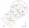 |
Fig. 1. HST-ACS mosaic (F818W filter) of MACS J0717.5+3745. Our targets are highlighted as red dots. The solid blue circle has a radius equal to r200, while the solid orange contour represents the weak-lensing mass reconstruction by Jauzac et al. (2012) (at a 3σ level) showing the cluster and its associated large-scale filament extending in the southeast direction. |
To increase the sample size, we include two other intermediate-redshift clusters, Cl 1416+4446 (z = 0.397) and Cl 0926+1242 (z = 0.489), in our analysis. For these intermediate-redshift clusters, the galaxy molecular gas reservoirs of three LIRGs was investigated by Jablonka et al. (2013).
In the following, the cluster masses, MΔ, are defined in the classical way, that is, as the mass enclosed within rΔ, the radius that encompasses a matter density Δ times larger than the critical density. The virial masses (M200) of Abell 2219, MACS J0717.5+3745, and Cl 1416+4446 have been inferred from weak-lensing analysis (Okabe et al. 2010; Israel et al. 2012; Medezinski et al. 2013). For these clusters we derived the r200 radius from M200 and estimated the concentration c200 at r200 from the concentration versus cluster mass relation by Duffy et al. (2008). For the other clusters M500 cluster masses inferred from X-ray analysis were reported by Jablonka et al. (2013), Haines et al. (2015), and references therein. We therefore iteratively used the relations by Duffy et al. (2008) and Hu & Kravtsov (2003) between the cluster mass (MΔ), concentration, and redshift to simultaneously estimate M200, r200, and the concentration c200.
Table 1 summarizes the cluster properties including the cluster mass, radius, and concentration outlined above. We also report the cluster center coordinates and velocity dispersions, which are obtained from the LoCuSS webpage1, as well as from previous studies (Ebeling et al. 2007; Jablonka et al. 2013; Haines et al. 2015).
Cluster properties.
2.2. Luminous infrared galaxies
We selected our targets primarily on the basis of their infrared (IR) luminosity, that is, log(LIR/L⊙) ≥ 11.2, to maximize the likelihood for a CO detection within eight hours of NOEMA integration time. The LIRGs were searched for in and around well-studied, intermediate-redshift clusters (see Sect. 2.1) up to two virial radii ∼2 r200. Our sample encompasses 17 LIRGs with accurate spectroscopic redshifts, 7 in the z ∼ 0.2 LoCuSS clusters and 10 in the HLS cluster MACS J0717.5+3745 at z ∼ 0.5.
In Fig. A.1 we show HST-ACS images of the 10 HLS MACS J0717.5+3745 cluster galaxies (F818W filter) as well as the source A2219-1 (F850LP filter). In Fig. A.2 we report Subaru images (i+, Ic bands) for the remaining 6 LIRGs in the Abell 697, 963, 1763, and 2219 clusters. High-resolution (∼0.2 kpc) HST images show, almost invariably, a presence of disturbed morphologies and clumpy substructures, likely associated with star-forming regions. From the Subaru images of the remaining LIRGs, at a resolution of 0.2 arcsec = (0.7−0.8) kpc, we perceive a central component (e.g., bulge, bar), from the more extended disk component, a few arcsec in size.
2.2.1. LIRGs in and around LoCuSS clusters
The targets in the LoCuSS clusters were initially selected on the grounds of existing Herschel PACS and/or SPIRE fluxes in addition to Spitzer 24 μm fluxes. Abell 1763, Abell 2219, and Abell 963 host two LIRGs each. In this study, we followed up these clusters for CO emission. Abell 697 has three LIRGs. So far we targeted only the brightest and closest LIRG to the cluster center for its outstanding property, namely A697-1. Indeed it is the most luminous cluster LIRG, nearly an ultra luminous infrared galaxy (ULIRG), over the full sample of 30 LoCuSS systems considered for follow up in CO, once the brightest cluster galaxies (BCGs) are excluded. This exclusion does not alter our results, since none out of the BCGs of the 6 LoCuSS/HLS clusters in our sample were detected by Herschel in the far-infrared (FIR) 100−500 μm range (Rawle et al. 2012). From the optical Subaru images, A697-1 appears to be a major merger; its IR emission peaks midway between the 2 galaxies.
2.2.2. LIRGs in and around MACS J0717.5+3745
The LIRGs of MACS J0717.5+3745 were selected after requiring detection in at least three Herschel bands. There are ∼18 such systems in and around MACS J0717.5+3745. From those we chose targets which could sample both the region inside the cluster virial radius and its filamentary structure, as shown in Fig. 1. The 10 target LIRGs of MACS J0717.5+3745 are either within the virial radius ∼r200 or belong to the extended filamentary structure toward the southwest. HLS071814+374117 is located in the outskirts of the cluster and is formally just outside the filamentary structure. Because this LIRG is located at r ∼ 1.5 r200 from the cluster center, the source fulfills the selection requirement r ≲ 2 r200 and it has been thus included in our sample of LIRGs.
2.2.3. Additional cluster LIRGs and the final sample
In the following we discuss the properties of additional LIRGs, with observations in CO from the literature, which have been included in our sample. We consider for our analysis 3 LIRGs from the clusters Cl 1416+4446 and Cl 0926+1242, which were detected in CO(2→1) or CO(1→0) by Jablonka et al. (2013). These 3 LIRGs have IR luminosities, inferred from the SED modeling, in the range log(Ldust/L⊙) = 11.1 − 11.5, which are similar to those of the other 17 new LIRGs considered in this work.
Moreover, in his doctoral dissertation, Cybulski (2016) reported 25 CO detections among Abell 963 members. By performing accurate SED modeling (see Sect. 3) in the FIR to UV wavelengths, we found only 1 source among the 25 with an estimated FIR luminosity > 1011 L⊙, typical of LIRGs, which has not been already included in our sample of LIRGs. Therefore we included this source, namely J101628.2+390932 at z = 0.211, in our analysis.
We also note that Cybulski et al. (2016) reported a CO detection for an additional cluster galaxy with an estimated FIR luminosity > 1011 L⊙. It is the Abell 2192 source J162644.6+422530 at z = 0.189, with a FIR luminosity log(LIR/L⊙) = 11.13 reported by the authors. However, it is located in the outskirts of the cluster and has not been included in our sample of LIRGs. The source has indeed a projected cluster-centric distance of 2.8 Mpc, corresponding to r/r200 = 1.9 (Verheijen et al. 2007).
Including the LIRGs of the above-mentioned publications yields a total sample of 21 LIRGs that are considered in this work. Table 2 lists the coordinates and cluster-centric distances of the LIRGs.
Properties of our targets.
The sample of LIRGs considered in this work is the largest sample of LIRGs in and around clusters at intermediate redshifts with CO detections. Our selection implies that each of the seven clusters considered in this work has at least one LIRG within the cluster virial radius to address any possible radial variation.
According to this constraint, we did not include in our sample the five intermediate-z LIRGs detected in CO(1→0) by Geach et al. (2011). We checked that they are indeed located well outside the virial radius, in the outskirts of the z ∼ 0.4 cluster Cl 0024+16: they are all at projected cluster-centric distances between (1 − 3)×r200 and three out of the five also have line-of-sight velocities > 3σcluster, relative to the cluster redshift.
3. Star formation rates and stellar masses
We consistently calculated SFRs and both stellar and dust masses of our new sample of LIRGs, based on FIR-to-UV photometry, wherever available. Stellar masses and SFRs have been derived with the Multi-wavelength Analysis of Galaxy Physical Properties (MAGPHYS) package (da Cunha et al. 2008), which enables self-consistent SED fits of both stellar and dust components. The calculations were performed with a Chabrier (2003) initial mass function (IMF) and are shown in Table 3. Figure 2 provides examples of SED fits. The LoCuSS galaxies have UV-to-FIR SEDs, which were obtained by combining GALEX, SDSS, UKIRT, Spitzer, and Herschel photometry. For the HLS sources belonging to MACS J0717.5+3745 we used CFHT U and Ks imaging, Subaru B, V, R, i, and z-band photometry, in addition to Spitzer and Herschel photometry. The SED fits of GAL0926+1242-A, GAL0926+1242-B, and GAL1416+4446 were done with griz, Ks in the NIR, Spitzer IRAC (3.6, 4.5, 5.8, 8.0 μm), and Spitzer MIPS (24 μm) fluxes.
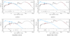 |
Fig. 2. Examples of FIR-to-UV MAGPHYS SED fits (solid black curve) for some of our targets. The galaxy IDs are indicated at the bottom of each panel. The photometric data points, corrected for Galactic extinction, are shown as red points. The solid blue curves show the SED fits in the absence of dust. Bottom panels: residuals. |
Results of the SED modeling.
Our SED fits are overall good, with χ2 values on the order of unity (Table 3). GAL0926+1242-B is an exception; this source has a higher χ2 = 21.9, mainly because of large i and z-band flux uncertainties (Fig. 2). Because of these uncertainties, it might be possible that the stellar mass estimate of GAL0926+1242-B is biased toward a lower value. However, removing this source from our sample would not change our conclusions. An output of MAGPHYS is also the dust luminosity Ldust, that is, the total stellar luminosity absorbed by dust in the stellar birth clouds and in the ambient interstellar medium, which is then reradiated. Therefore, Ldust is a physically motivated analog of the total observed IR luminosity LIR. From the best-fit results reported in Table 3 the dust luminosities are found in the range log(Ldust/L⊙)≃11.1 − 11.8, and are thus consistent with the fact that the galaxies are LIRGs, for which it holds log(LIR/L⊙)≃11 − 12.
4. Molecular gas
4.1. Observations
The 17 new LIRGs in our sample were observed in CO with the IRAM Plateau de Bure interferometer (PdBI; Guilloteau et al. 1992; Cox 2011) and its successor NOEMA (Schuster 2014). Observations were carried out between 2012 and 2017 as part of five programs: W036, X2D, S14BU, S17BI, and W17CX (PI: Jablonka). The summary of these observations is presented in Table 4.
Summary of the PdBI/NOEMA observations.
At a resolution of a few arcsec, all our targets were unresolved by the observations. Data reduction was performed using the GILDAS package2. Data were calibrated using the standard pipeline adopting a natural weighting scheme to maximize sensitivity.
4.2. CO fluxes
The CO fluxes from our NOEMA observations were calculated following the procedure described in Castignani et al. (2018), which provides further details. Each spectrum is fitted using a χ2 minimization procedure with a best-fit model given as the sum of a polynomial of degree one and a Gaussian to account for both the baseline and the CO emission line of each target. The significance of the CO detection is assessed by a Monte Carlo simulation of N = 1000 spectra per target, which are then fitted with the same χ2 minimization procedure described above. The velocity integrated SCO(J → J − 1)Δv flux, in units of Jy km s−1, is calculated by integrating the Gaussian model to the simulated spectrum. For each source we then used the median and the 68.27% confidence region of the flux distribution to get the velocity integrated flux and its 1σ uncertainty.
Velocity integrated fluxes were then converted into velocity integrated luminosities  , in units of K km s−1 pc2, using Eq. (3) of Solomon & Vanden (2005), that is,
 (1)
(1)
where νobs, in GHz, is the observer-frame frequency of the CO(J → J − 1) transition, DL is the luminosity distance in Mpc, and z the redshift.
Our NOEMA observations yield 15 CO detections out of 17 targets. For HLS071760+373709 and HLS071805+373805, in the outskirts of MACS J0717.5+3745, we did not find any CO emission associated with the 2 LIRGs, after carefully inspecting their data cubes. Therefore, for these 2 LIRGs we set 3σ upper limits ≲0.5 Jy km s−1 for the CO(2→1) flux, at 300 km s−1 resolution in velocity. Throughout this work we remove these 2 sources when estimating statistical quantities of our sample that are related to CO. Concerning the other 4 sources in our sample, from the literature, the SCO(J → J − 1) fluxes of GAL0926+1242-A, GAL0926+1242-B, and GAL1416+4446 are from Jablonka et al. (2013), while that of J101628.2+390932 is from Cybulski (2016), which we refer to for further details. Table 5 summarizes the results.
Molecular gas properties.
Figures A.1 and A.2 show the HST and Subaru images of our targets, together with the CO contours. Figure A.3 shows the CO intensity maps and the corresponding spectra. The CO emission peak of A697-1 is slightly shifted toward its southern companion, which is consistent with a similar offset found in the IR map (see also Sect. 2.2).
Interestingly, Cybulski et al. (2016) observed 5 galaxies belonging to Abell 963 in CO(1→0) with the Large Millimeter Telescope (LMT). Their sample includes A963-2, for which the authors report a velocity integrated flux of SCO(1 → 0)Δv = (1.771 ± 0.348) Jy km s−1, consistent with that independently estimated in this work,  Jy km s−1.
Cybulski (2016) also includes A963-1, with an estimated SCO(1 → 0)Δv = (2.290 ± 0.437) Jy km s−1. For this source, we obtained a lower flux  Jy km s−1, at higher signal-to-noise ratio, S/N = 7.7 versus S/N = 5.2 reported by Cybulski (2016). We suggest that the flux discrepancy may be due to the underestimated uncertainty for the LMT observations: our interferometric data likely have a more stable spectral baseline compared to the single-dish LMT data. We note that S/N ≃ 5 detections are somehow uncertain, even with ALMA (Walter et al. 2016; Decarli et al. 2016).
4.3. Molecular gas masses
We estimated the total molecular gas masses of our targets as  , where
  is the excitation ratio. In this work the CO(2→1) and CO(1→0) transitions are considered and we assumed r21 = 0.85, typical of submillimeter galaxies (Carilli & Walter 2013, for a review).
As reported in Table 3 our targets span a broad range of SFRs, from ∼0.5 × SFRMS up to ∼10 × SFRMS, where SFRMS is the SFR at the main sequence (MS) estimated following the Speagle et al. (2014) prescription.
By only assuming a Galactic CO-to-H2 conversion factor XCO ≃ 2 × 1020 cm−1/(K km s−1), that is, αCO = 4.36 M⊙ (K km s−1 pc2)−1, typical of MS galaxies that commonly have SFR ≲ 3 × SFRMS (Solomon et al. 1997; Bolatto et al. 2013), we could potentially overestimate the molecular gas masses of our most active sources, that is, well above the MS (see, e.g., Noble et al. 2017; Castignani et al. 2018, for a discussion). A value of αCO ≃ 0.8 M⊙ (K km s−1 pc2)−1 is typically assumed for highly star-forming sources such the ULIRGs (Bolatto et al. 2013, for a review). Since our sample includes sources with SFR both within and above the MS, we adopt the following heuristic prescription for the CO-to-H2 conversion factor, unless specified otherwise:
 (2)
(2)
where  . The adopted αCO conversion factor can be linearized for x ≳ 0 as
  . The αCO(SFR) prescription was chosen in such a way that αCO corresponds to the Galactic value for SFR ≲ SFRMS, while it asymptotically declines, with no discontinuity, down to αCO = 0.8 M⊙ (K km s−1 pc2)−1 for SFR ≫ SFRMS.
Our SFR-dependent prescription is heuristic and adopted in this work to partially circumvent the problem of choosing appropriate values of αCO for both MS and more star-forming LIRGs. According to Eq. (2) galaxies with  , 3, and 10 have
  , 3.65, and 2.11, respectively. Similarly, for the targeted LIRGs, the resulting αCO varies within the range (2.16 − 4.36) M⊙ (K km s−1 pc2)−1, safely above αCO ≃ 1 M⊙ (K km s−1 pc2)−1, which is indeed typical of ULIRGs. The impact of the choice of αCO is discussed in Sect. 6.2.
4.4. Gas fraction and depletion timescale
We calculated the gas depletion timescale, τdep = MH2/SFR, associated with the consumption of the molecular gas and the molecular gas to stellar mass ratios, M(H2)/M⋆, from the galaxy stellar masses and the SFRs from our SED fits and the galaxy molecular gas mass estimates, which we introduced in previous sections.
The molecular gas properties of J101628.2+390932 (Cybulski 2016), M(H2) and τdep, have been estimated analogously to the other sources in our sample. To this aim, for this source we adopted SCO(1 → 0)Δv = (1.250 ± 0.313) Jy km s−1 (Cybulski 2016) and αCO = 3.25 M⊙ (K km s−1 pc2)−1, using Eq. (2).
For comparison we also estimated the depletion time τdep, MS and the molecular gas fraction  for the MS field galaxies with redshifts and stellar masses corresponding to those of our targets, following the Tacconi et al. (2018) prescription.
5. Comparison samples
In order to place the properties of our LIRGs into context, we compiled published datasets of field and cluster star-forming galaxies, both in the local and distant Universe, that have been observed in CO. In particular, as outlined below, the distant star-forming galaxies that are used for our comparison include a homogeneous compilation of sources out to z ≃ 1.6, largely in the field, or at most in the cluster outskirts (Geach et al. 2011).
As in Jablonka et al. (2013) for our comparison we include field and cluster galaxies in the local Universe, which have been observed in CO and also benefit from IR luminosities and stellar mass estimates (Kenney & Young 1989; Casoli et al. 1991; Young et al. 1995; Boselli et al. 1997; Lavezzi & Dickey 1998; Lavezzi et al. 1999; Helfer et al. 2003; Gao & Solomon 2004; Kuno et al. 2007; Saintonge et al. 2011; García-Burillo et al. 2012; Scott et al. 2013). In line with our sample we restrict the comparison to galaxies with stellar masses log(M⋆/M⊙) > 9.5 and FIR luminosities in the range log(LIR/L⊙) = 9 − 12. Since we are mainly interested in looking for a possible cosmological evolution of galaxy properties, we also remove local sources stricto sensu, that is, we only consider galaxies with z > 0.01. This selection yields a total of 154 sources, all at z < 0.054: 79 field galaxies, with  and
and  , as well as 75 cluster galaxies, with
  and
and  3.
3.
We consider the 61 star-forming galaxies at 0.15 < z < 0.35 from the Herschel Astrophysical Terahertz Large Area Survey (H-ATLAS) with ALMA CO(1→0) detections reported by Villanueva et al. (2017). They have total IR luminosities and stellar masses in the range log(LIR/L⊙)≃10.1 − 11.9 and log(M/M⋆)≃9.7 − 11.3, respectively, which were estimated using SED fits with MAGPHYS, similar to what has been done for our work. We did not consider 6 sources with only upper limits in CO(1→0) that are part of the full sample of 67 galaxies reported in Villanueva et al. (2017).
For the studies quoted above, the galaxy IR luminosities were converted into SFRs using the Kennicutt (1998) relation, rescaled for a Chabrier (2003) IMF, on which MAGPHYS SED fits of this work relies. Namely, following the prescription by da Cunha et al. (2010) we adopted the relation
 (3)
(3)
We further include the following samples.
– The five LIRGs detected in CO(1→0) by Geach et al. (2011) in the outskirts (r/r200 ∼ 1 − 3) of the rich cluster Cl 0024+16 (z = 0.395). The authors report 7.7μm-based SFRs in the range ∼(30 − 60) M⊙ yr−1 and stellar masses M⋆ ∼ 1011 M⊙.
– The sample of 20 LIRGs at 0.2 < z < 0.7 detected in CO(3→2) with ALMA observations by Lee et al. (2017). The sources fall within the equatorial COSMOS survey (Scoville et al. 2007) and are bright submillimeter galaxies observed with Herschel. These have IR luminosities log(L/LIR)≃11.1 − 11.6 and SFR ≃ (10 − 37) M⊙ yr−1. Estimates for the SFR were obtained by the authors using both IR and UV luminosities using data from Spitzer, Herschel, and GALEX.
– The subsample of 27 star-forming galaxies, SFR = (3.4 − 106) M⊙ yr−1, at z = 0.05 − 0.3, with CARMA observations in CO(1→0) by Bauermeister et al. (2013). Our selection excludes their 4 z ≃ 0.5 sources with upper limits only in CO(3→2). We adopt stellar masses and SFRs reported by the authors that correspond to those of the seventh release of SDSS provided by the Max-Planck-Institute for Astrophysics-John Hopkins University (MPA-JHU) group4.
– The 8 z = 0.1 − 0.2 star-forming galaxies detected in CO(1→0) by Morokuma-Matsui et al. (2015) with the Nobeyama Radio Observatory (NRO). We adopt the SFRs, SFR ≃ 10 M⊙ yr−1, reported by the authors, which correspond to those of the tenth release of the SDSS5 and were derived using at least five emission lines (Brinchmann et al. 2004).
– The recent PHIBSS2 observations from Freundlich et al. (2019). Their sample includes 60 CO(2→1) detections of 0.5 < z < 0.8 star-forming galaxies, with SFR = (28 − 630) M⊙ yr−1, inferred from UV and IR fluxes, and corrected for extinction.
– Tacconi et al. (2013) present 52 CO(3→2) detections of star-forming galaxies in two redshift slices centered at z ∼ 1.2 and 2.2. The observations are part of the Plateau de Bure high-z Blue Sequence Survey (PHIBSS) and were done with the PdBI. For our comparison we consider the subsample of 38 detections at 1.0 ≲ z ≲ 1.5 with SFR = (28 − 630) M⊙ yr−1, estimated by the authors and based either on the sum of the observed UV and IR luminosities, or on an extinction-corrected Hα luminosity. In both cases the SFRs provided by the authors were corrected for a Chabrier (2003) IMF, hence consistent with our estimates.
– The six BzK field galaxies detected in CO by Daddi et al. (2010), at 1.4 < z < 1.6 with estimated IR luminosities LIR = (0.6 − 4.0)×1012 L⊙, typical of ULIRGs. The SFRs, (62−400) M⊙ yr−1, were calculated with a Chabrier (2003) IMF, hence consistent with our estimates. Likewise Tacconi et al. (2013) we include these six sources in the PHIBSS sample.
6. Results
6.1. Stellar masses and star formation rates
In Fig. 3 we report, as a function of redshift, the SFRs, stellar masses, and molecular gas to stellar mass ratios of the LIRGs in our sample and those of the galaxies in the comparison samples. As seen in Fig. 3a, our sources have SFRs in the range ≃(4 − 50) M⊙ yr−1, with values typical of intermediate-redshift MS galaxies within the same mass range (log(M⋆/M⊙)≃10 − 11), as displayed in Fig. 3b, which shows the galaxy stellar mass as a function of redshift.
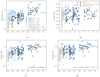 |
Fig. 3. a: SFR vs.z and b: M⋆vs.z scatter plots. The green dotted line in panel a shows the empirical SFR values by Speagle et al. (2014) for MS field galaxies (SFRMS) with stellar mass log(M⋆/M⊙) = 10.6, which corresponds to the mean stellar mass for the LIRGs in our sample. c,d: molecular gas to stellar mass ratio as function of redshift; the two plots differ in terms of the adopted αCO, as shown at the bottom right of the panels. The green dotted lines show the empirical values found by Tacconi et al. (2018) for MS field galaxies with a stellar mass log(M⋆/M⊙) = 10.6. The color code for the data points is given in panels a,b. |
At fixed stellar mass, our LIRGs, however, have lower SFRs than the more distant 1.0 < z < 1.6 sources (Daddi et al. 2010; Tacconi et al. 2013) in the comparison sample. This is the consequence of the increment of the SFR at the MS with redshift, as shown in Fig. 4a, where the SFR versus stellar mass scatter plot is shown, along with the MS relation at different redshifts.
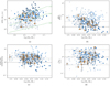 |
Fig. 4. a: star formation rate as a function of stellar mass, the MS relation at different redshifts from Speagle et al. (2014) is shown as dotted green lines. b–d: SFR, molecular gas to stellar mass ratio, and depletion time, respectively, all normalized by the corresponding MS values (Speagle et al. 2014; Tacconi et al. 2018), as a function of the stellar mass. The color code for the data points is analogous to Fig. 3. Panels b–d: the horizontal dashed line refers to the MS value, that is, the y-axis value equal to unity, while the horizontal dotted lines show the range of y-axis values corresponding to MS galaxies. |
Once SFRs are normalized to the corresponding MS values (Fig. 4b), our LIRG sample populates the same region in the SFR/SFRMS versus log(M⋆/M⊙) diagram as the comparison sample sources, irrespective of their SFR, from normal star-forming galaxies to LIRGs, as well as distant ULIRGs (Daddi et al. 2010). We also note that the comparison sources preferentially lie on the upper part of the MS. This is most likely an observational bias and is linked to the fact that CO observations for SFR < SFRMS sources are more uncertain and require a longer integration time.
Figure 4b shows a significant scatter in SFR/SFRMS, or equivalently in sSFR/sSFRMS, at a given log(M⋆/M⊙). Most of our LIRGs are distributed within the fiducial |log(SFR/SFRMS)| < log(3) = 0.48 scatter of the MS, with the exception of 8 LIRGs that have a higher level of star formation activity (see also Table 3). No strong trend is observed between SFR and stellar mass, as indeed low SFRs are seen both at the low- and the high-mass ends of our sample, although the most active of our systems have log(M⋆) ≤ 10.5. This last aspect is reflected in a tentative anticorrelation, with a significance of 2.5σ (p-value = 0.013), between SFR/SFRMS and log(M⋆/M⊙), that we find with the Spearman test.
Furthermore, despite the LIRGs in our sample having been primarily selected on the basis of their FIR luminosity, they span a relatively wide range (an order of magnitude) in SFR, which is because both FIR and UV luminosities are useful to constrain the SFR. This can be appreciated from the comparison between the SEDs of A1763-1 and A2219-1 in Fig. 2. While A1763-1 is brighter in the FIR, it also has a lower SFR than A2219-1. This is ultimately because A2219-1 has a stronger UV excess (GALEX, Morrissey et al. 2007), as seen in the SEDs. We also stress that using the total IR as a SFR tracer may lead to an overestimation of the SFR, unless the contribution by the diffuse interstellar medium to the total IR luminosity is properly taken into account (see also discussion in Kennicutt et al. 2009; da Cunha et al. 2012; Hayward et al. 2014; Hunt et al. 2019). For the LIRGs in our sample, we find that by using Eq. (3), with LIR replaced by Ldust provided by MAGPHYS, the SFR is  higher6 than that estimated by MAGPHYS (Table 3) using the full FIR-to-UV SED.
6.2. Molecular gas and depletion timescale
In Figs. 3c,d we show the redshift evolution of the molecular gas to stellar mass ratio μ = M(H2)/M⋆ and illustrate the impact on μ when choosing different αCO prescriptions. The majority (13) of the LIRGs have SFR/SFRMS ≲ 3 and are therefore formally consistent with being on the MS. Among the remaining eight LIRGs, half of them have SFR/SFRMS ≃ (3 − 4) and the other half have SFR/SFRMS ≃ (6 − 10). To account for such a broad range in SFR, from the MS up to larger values, in Sect. 4.3 we have introduced a heuristic dependence of αCO on the SFR, denoted as αCO(SFR) prescription. In panel c of Fig. 3 the values of μ are estimated using this prescription, while in panel d a Galactic H2-to-CO conversion factor αCO = 4.36 M⊙ (K km s−1 pc2)−1 is used.
Large differences in μ between the two prescriptions, up to a factor of ∼5 in molecular gas masses are seen, but only in the case of very active and gas rich systems with μ ≳ 1. However, the discrepancy in μ for normal star-forming galaxies and LIRGs is limited and does not exceed a factor of ∼2.
Our sample of LIRGs covers a factor ∼30 in SFR and shows a small but clear increase of star formation activity from  yr−1 at z ∼ 0.25 to
  yr−1 at z ∼ 0.5 following standard relations for MS galaxies (e.g., Speagle et al. 2014)7.
On the other hand, the LIRGs span a lower factor ∼7 in μ, with an increment going from  at z ∼ 0.25 to
  at z ∼ 0.5, following the general trend driven by standard relations for MS galaxies (Tacconi et al. 2018). Furthermore, while the SFRs cover the full range of SFRs reported so far in the literature at similar redshifts (Fig. 3a), the molecular gas to stellar mass ratios of our LIRGs seem to lie in the high tail of the distribution (Fig. 3c). However, by applying standard nonparametric tests (Mann-Whitney-Wilcoxon, Kolmogorov-Smirnov) we did not find any statistically significant difference in the distributions of μ between our LIRGs and sources in the comparison sample at similar redshifts 0.2 < z < 0.6 than the LIRGs.
In Figs. 4c,d we compare the ratios μ and the depletion timescale τdep = M(H2)/SFR, both normalized to their values at the MS, of the LIRGs in our sample with those of the sources in the comparison samples. The normalized μ and τdep are plotted against the stellar mass on the x-axis.
Our LIRG sample shows normalized values of μ equal to  and therefore covers the upper part of the range typically associated with MS galaxies (Tacconi et al. 2018). However, our sample of LIRGs does not contain any extremely gaseous system, with normalized values of μ in the range ∼(0.8 − 3.6), that is, a factor of ∼4 dispersion.
As shown in Fig. 4b a much larger dispersion is observed for the normalized SFR, SFR/SFR . The normalized SFR spans indeed the range between ∼(0.5 − 9.6), corresponding to a factor of ∼20 dispersion, which is much higher than that found for the normalized μ.
As seen in Fig. 4d and Table 5 depletion times within τdep = (0.3 − 5) Gyr are found for the targeted LIRGs, with values scattering around those associated with the MS and equal to  . Similarly to what has been found for the SFR (Sect. 6.1), by applying the Spearman test a hint for a correlation between the normalized τdep and log(M/M⋆) is found at 2.5σ (p-value = 0.014). The location of the LIRGs in the normalized τdep versus log(M⋆/M⊙) plane reflects the trend observed in the SFR/SFRMS versus log(M⋆/M⊙) plot in Fig. 4b. This is a result of the flat behavior of the normalized μ with M⋆ and its relatively small dispersion. Therefore, the small timescales τdep < τdep, MS observed for a large fraction of our LIRGs (i.e., 13 out of 21) are the result of stronger activity rather than exhaustion of gas.
Overall, the results presented in Figs. 3 and 4 show that the present study is one of the first to probe statistically large molecular gas reservoirs in the still overlooked population of star-forming cluster galaxies at intermediate redshifts. Our results thus complement, in terms of redshift and environment, those found for field galaxies, and also those of star-forming cluster or field galaxies in the local Universe, of which the LIRGs in our sample are the higher-z counterparts.
6.3. Galaxy properties versus cluster-centric distance
In the following we focus on the properties of our sample of intermediate-redshift LIRGs in Abell 1763, Abell 2219, Abell 697, Abell 963, Cl 0926+1242, Cl 1416+4446, and MACS J0717.5+3745 (Tables 2, 3, and 5).
Figure 5 (left) suggests that the SFR/SFRMS = (SFR/M⋆)/(SFRMS/M⋆) = sSFR/sSFRMS values scatter within the MS range. However, while the inner regions of clusters (i.e., r/r200 < 0.6) contain galaxies with normal star formation activity, all LIRGs formally above the MS, with SFR > 3 × SFRMS, are found within the cluster virial radius, irrespective of the cluster redshift. Among the 16 LIRGs in our sample with projected cluster-centric distances < r200, 7 (44%±12%)8 have enhanced SFR > 3 × SFRMS.
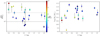 |
Fig. 5. Star formation rate to SFRMS (left panel) and stellar mass (right panel), as a function of r/r200 of the LIRGs. Symbols are shown as in Fig. 3b. Blue, green, yellow, and red data points correspond to increasing SFR/SFRMS values, as illustrated in the color bar (left). Left panel: the horizontal dashed line refers to the MS value, while the horizontal dotted lines show the ±0.48 dex scatter corresponding to MS galaxies. |
As seen in the right panel of Fig. 5 these cluster-core, star-forming galaxies tend to have lower stellar masses, log(M⋆/M⊙) < 10.6, than the rest of the LIRGs. However the stellar mass alone is not a sufficient criterion to explain the high star formation activity in the cluster-core LIRGs. For example, both GAL0926+1242-A and A2219-2 are on the MS and have low stellar masses, log(M⋆/M⊙)≃(10.3 − 10.4). Similarly, the two MACS J0717.5+3745 LIRGs at the very upper edge of the MS have log(M⋆/M⊙)≳10.8. We statistically quantified our results. By applying the Spearman test we found a tentative anticorrelation that has a significance of 2.2σ (p-value = 0.03), between SFR/SFRMS and r/r200, which is ultimately due to the presence of LIRGs with SFR > 3 × SFRMS in the cluster inner regions. However, we stress that additional observations in CO of LIRGs in the cores of intermediate-redshift clusters are needed to strengthen our results.
Figure 6 places our sample in the cluster phase-space (line-of-sight velocity versus cluster-centric radius) diagram. The LIRGs are color coded according to their SFR/SFRMS ratios. We also highlight the smallest and largest virialized regions in dark and light gray, respectively, accounting for the different cluster masses and concentrations of the clusters considered. The virialized regions were derived with the analytical model of Jaffé et al. (2015). Our targets span a broad range of cluster-centric distances, from the cluster cores to their infall regions, out to ∼1.6 r200. Most of the sample LIRGs are overall located within the cluster virialized region; the line-of-sight velocity is not greater than ∼2 times the cluster velocity dispersion.
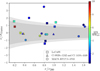 |
Fig. 6. Phase space diagram for all cluster galaxies in our sample. In the x-axis we plot the projected cluster centric radius, r, normalized to r200, while in the y-axis we plot the line-of-sight velocity, normalized to the cluster velocity dispersion σcluster. The dark and light gray areas show the range of virialized regions defined by Jaffé et al. (2015) for the clusters in our sample. |
Interestingly, two LIRGs in MACS J0717.5+3745, which have projected cluster-centric distances below r200 but normal SF activity (SFR/SFRMS < 3) have relative velocities larger than 2σcluster. Large velocities are often found for cluster-core members; this also applies to MACS J0717.5+3745 (σcluster ≃ 1660 km s−1; Table 1). Considering these aspects, the location of the two sources with respect to the cluster center does not significantly differ from that of the LIRGs in our sample with lower values of v/σcluster, but higher cluster centric distances r > r200. Thus the two LIRGs likely belong to the infall regions of MACS J0717.5+3745 and we have not discarded them, although these two LIRGs are formally outside the virialized region of the cluster (Fig. 6).
The left panel of Fig. 7 shows that the factor ∼4 dispersion in the normalized μ that was noted in Sect. 6.2 from Fig. 4c has no clear link with the spatial position of the galaxy. A similar behavior is found for the H2-to-dust mass ratio, as a function of r/r200. On average we find  , which is consistent with the typical ratio ∼100 found for star-forming galaxies (Scoville et al. 2014, 2016; Berta et al. 2016). However, interestingly, as seen in Fig. 7 (right), when both molecular gas and star formation activity are considered together via the gas depletion timescale, τdep, a deficit of sources with τdep ≳ τdep, MS is observed, as we move from the outskirts r ≳ r200 down to the cluster inner regions.
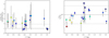 |
Fig. 7. Molecular gas to stellar mass ratio (left) and depletion time (right), normalized to the corresponding MS values, as a function of r/r200. The data points have different symbols and are color-coded according to the corresponding SFR/SFRMS, as in Fig. 6. In each panel, the horizontal dashed line refers to the MS value, while the horizontal dotted lines show the range of y-axis values corresponding to MS galaxies. |
This radial trend stands out more clearly than in the case of SFR/SFRMS versus r/r200 (Fig. 5, left panel). The Spearman test suggests a possible correlation between τdep/τdep, MS and r/r200, which we find at a significance of 2.8σ (p-value = 0.005) despite the significant scatter of τdep/τdep, MS at a given cluster-centric distance.
7. Discussion
7.1. Star formation enhancement and gas enrichment
For this work we selected a sample of LIRGs based on their FIR luminosities. However, once we modeled their FIR-to-UV SEDs the LIRGs show a wide range in SFR ≃ (4 − 50) M⊙ yr−1, which is a result of the combination of both obscured (in the FIR) and unobscured (in the UV) ongoing star formation activity.
The presence of enhanced star formation activity observed in a large fraction of the LIRGs within the virial radius suggests that environmental processing mechanisms such as ram-pressure stripping, galaxy harassment, and starvation may have not been sufficiently effective in suppressing the star formation and then quenching the LIRGs. Recent simulations of dwarf galaxies by Hausammann et al. (2019) show that, at variance with the hot gas, cold gas may not be efficiently removed by ram pressure.
Our results suggest that the enhancement of star formation for the cluster LIRGs, toward the cluster cores, is the main responsible for the corresponding decrease of depletion timescales (i.e., τdep ≲ τdep, MS). The short depletion times imply that the star formation in the LIRGs is shortly suppressed, which ultimately quenches them, meanwhile increasing the fraction of passive galaxies in clusters (e.g., SFR versus density and morphology versus density relations, Dressler 1980; Lewis et al. 2002; Peng et al. 2010; Andreon et al. 2006; Raichoor & Andreon 2012). The short depletion times observed for a large fraction of LIRGs within the virial radius also imply that molecular gas is consumed rapidly in cluster LIRGs. This may help to explain the fast exponential decrease with time, since z ∼ 0.8 of the fraction of LIRGs in clusters found in previous studies (Finn et al. 2010; Saintonge et al. 2008; Popesso et al. 2012).
To further investigate this scenario it is interesting to look for possible differences among the LIRGs, in terms of denser molecular gas reservoirs, from those probed by the low J = 2 → 1 and J = 1 → 0 transitions of CO considered in this work.
Visual inspection of the images of our LIRGs (Figs. A.1 and A.2) also suggests the presence of compact or clumpy optical morphologies, which seem to be common in distant star-forming and Herschel-selected galaxies. Consistent with these results, using ALMA observations Puglisi et al. (2019) recently found that a significant fraction, that is, ∼50%, of their sample comprising 93 Herschel-selected galaxies at 1.1 ≤ z ≤ 1.7 and at the MS show a compact morphology. The authors interpret their sources as early post-starburst galaxies.
7.2. Gas compression and environmental processing
Similar to the targeted LIRGs of this work, star-forming galaxies have been occasionally found in the cores of nearby clusters in previous studies. Miller & Owen (2001) found an excess of star-forming galaxies with enhanced radio emission, possibly not due to active nuclei, in the cores of nearby Abell clusters. Bressan et al. (2002) proposed that this excess could be associated with a population of starburst galaxies. Miller & Owen (2001) proposed instead that the excess is due to compression of the galactic magnetic field by thermal pressure of the intra-cluster medium, while Gavazzi & Jaffe (1986) suggested that the excess is due to the ram pressure, which ultimately strengthens the magnetic field of the galaxy, as it moves through the intra-cluster medium. Overall, the compression of gas is invoked in these studies to explain the excess of star-forming galaxies in the cores of nearby clusters. Consistent with these studies, simulations by Bekki (2014) found that the ram pressure can compress the interstellar medium gas and ultimately enhance the star formation of cluster and group galaxies. In the following we investigate the possibility that gas compression is also responsible for the strong star formation activity in some of the targeted LIRGs.
A2219-1 is close to the shock front of A2219, which might have favored the gas compression and an enhancement of star formation in the galaxy. The galaxy has a high SFR = 21.2 M⊙ yr−1, corresponding to SFR ≃ 18 SFRMS, which is strengthened by its UV excess (Fig. 2). Similarly, for A2744 at z = 0.308, which is part of the HLS project, Rawle et al. (2014) found that cluster sources with elevated SFR could be associated with a large-scale shock front, suggesting gas compression as the cause.
A large fraction ∼50% (10/21) of the LIRGs in our sample belong to MACS J0717.5+3745. Seven among the ten LIRGs are formally located within the r200 radius, in projection, while HLS071760+373709, HLS071805+373805, and HLS071814+374117 are found at larger cluster-centric distances (see Table 2). As shown in Fig. 1 the LIRGs follow the pattern in dark matter defined by the weak-lensing analysis by Jauzac et al. (2012). In particular, the three LIRGs at projected cluster-centric distances > r200 fall within the filament extending toward the southeast from the cluster core.
We did not find any statistically significance difference concerning the molecular gas content of the MACS J0717.5+374 LIRGs from the cluster inner regions out to the outskirts; see Fig. 7 (left). This result suggests that there is no strong evidence of preprocessing of molecular gas in these LIRGs by the large-scale dense environment (cluster and filament). However, the MACS J0717.5+374 LIRGs contribute to the observed increase of τdep, normalized to its MS, with increasing cluster centric distances (Fig. 7, right), which has been discussed in Sect. 6.3 and is primarily due to the increase of the normalized SFR toward the cluster core.
Interestingly, we found four MACS J0717.5+3745 LIRGs, namely HLS071754+374303, HLS071731+374250, HLS071740+374755, and HLS071814+374117 at the edge of both X-ray and radio extended emissions associated with the cluster (see Fig. 1 of Bonafede et al. 2018). HLS071754+374303 is also close to an X-ray infalling group to the southeast of the cluster, along the filament. The four sources have SFR ≳ 30 M⊙ yr−1 and are therefore among those in our sample with the strongest star formation activity. Furthermore, while HLS071740+374755 is located to the northeast of the cluster, the other three LIRGs are all found along the filament direction and also formally above the MS, having SFR ≳ 3 SFRMS.
To explain such high (normalized) SFRs a possible scenario may be that a large-scale shock in MACS J0717.5+374 has compressed the gas reservoirs in some of the LIRGs along the filament direction thus ultimately enhancing their star formation activity. Interestingly, previous studies suggested that the ∼(0.7 − 0.8) Mpc radio relic found in MACS J0717.5+374 (Bonafede et al. 2018) traces a large-scale shock wave propagating through the cluster and originated from either the merger events (van Weeren et al. 2009) or an accretion shock related to the SE filament (Bonafede et al. 2009).
Nevertheless, we note that HLS071708+374557 is highly star forming and has SFR ≃ 40 M⊙ yr−1 ≃ 6 SFRMS. However, it is not found in correspondence of the X-ray or radio emission of the cluster. As further outlined below it is thus likely that shock-induced gas compression is not the only mechanism possibly responsible for the high star formation activity observed in the LIRGs of MACS J0717.5+374.
Interestingly, the only two sources with only upper limits to the CO flux have a normal MS star formation activity and are both located at the periphery (r/r200 ≃ 1.6) of MACS J0717.5+374. These two sources might be backsplash galaxies that have already experienced the processing by the cluster environment and are thus depleted in CO, similar to what was found in simulations by Bahé et al. (2013).
By summing up the SFRs of the seven MACS J0717.5+374 LIRGs with projected cluster-centric distances < r200 we derive lower limits to the total SFR of the cluster, SFR ≳ 227 M⊙ yr−1, and to the SFR normalized to the cluster mass, SFR/M200 ≳ 8 × 10⁻¹⁴ yr−1. The latter estimate makes MACS J0717.5+3745 among the clusters at intermediate redshift with the highest SFR, normalized to the cluster mass (e.g., Finn et al. 2005; Geach et al. 2006; Haines et al. 2009b; Chung et al. 2010)
Similar to what was proposed by Chung et al. (2010) for the Bullet cluster and by Fadda et al. (2008) for Abell 1763 the significant normalized star formation activity of MACS J0717.5+3745 might be explained if its LIRGs, or a fraction of them, belong to a population of infalling galaxies, possibly associated with the filament, that have not been quenched yet. If this is the case, the accretion timescale is not greater than a few hundred million years in order to be shorter than the depletion timescale τdep ≃ (0.3 − 1.3) Gyr needed to quench the selected LIRGs of MACS J0717.5+3745.
For our environmental study we considered the location of the LIRGs in the cluster, parameterized by means of their r/r200 (e.g., Figs. 5–7). While it would have been more appropriate to parameterize the effect of the environment by means of the local density (e.g., Dressler 1980; Peng et al. 2010), to account for cluster substructures, this analysis requires a complete spectroscopic census of the cluster members, which is however very difficult to obtain, from the core out to the periphery of distant clusters.
8. Conclusions
We investigated the role of dense Mpc-scale environments in processing the molecular gas in galaxies as part of a larger search for CO in distant cluster galaxies. To this aim we considered a sample of 17 cluster galaxies at intermediate redshifts z ∼ 0.2 − 0.5 with available FIR-to-UV photometry, as well as high-resolution images from Subaru and HST. The galaxies were selected for having total IR luminosities ≳1011 L⊙, which classify the sources as LIRGs. The sources belong to well-studied clusters (Abell 697, 963, 1763, 2219, and MACS J0717.5+3745) from the LoCuSS and HLS surveys. The LIRGs also span a broad range in cluster centric distances, out to ∼1.6 × r200, and are therefore an optimal sample to study the preprocessing of gas as the galaxies in the outskirts of clusters fall into their cores.
We observed the LIRGs in CO(1→0) or CO(2→1) with several observational programs carried out between 2012 and 2017 with the IRAM PdBI and its successor NOEMA. The sample of 17 LIRGs has been complemented with 4 additional cluster LIRGs, 3 of which have already been observed in CO by Jablonka et al. (2013), and the fourth by Cybulski et al. (2016). Accurate multiwavelength SED modeling from the FIR to UV was performed for all 21 LIRGs, which has allowed a homogeneous analysis of the full LIRG sample.
We compared the SFRs, molecular gas to stellar mass ratios M(H2)/M⋆, and depletion times of the LIRGs with, first, those estimated using empirical relations for MS field galaxies and, second, those of a compilation of galaxies from the literature, out to z ≃ 1.6. Our analysis suggests that the targeted LIRGs have SFRs, molecular gas contents, and depletion times that are consistent with those of both MS field galaxies and star-forming galaxies from the comparison sample, independent of the stellar mass considered, within log(M⋆/M⊙)≃10 − 11.
However, a 2.8σ correlation between the depletion time, normalized to the value at the MS, and the projected cluster-centric distance, in units of r200, is found for the sample of LIRGs. The correlation is ultimately due to an increase of SFR from a few M⊙ yr−1 in the cluster outskirts up to ∼50 M⊙ yr−1 in the inner regions r ≲ 0.4 r200 of the clusters. Indeed, a large fraction of our cluster LIRGs, 7 out of the 16 LIRGs in our sample with projected cluster-centric distances < r200, that is, 44%±12%, have enhanced SFR > 3 × SFRMS. On the other hand, the ratio M(H2)/M⋆ ≃ (0.2 − 1) scatters around the MS value with no observed trend as a function of the cluster-centric distance, neither of the stellar mass.
We discussed possible scenarios to explain the presence of significant large reservoirs of molecular gas in the LIRGs from the outskirts down to the cluster cores as well as the rising of the star formation with decreasing cluster-centric distance. The presence of enhanced star formation activity observed in a large fraction of the LIRGs within the virial radius suggests that environmental processing mechanisms such as ram-pressure stripping, galaxy harassment, and starvation may have not been sufficiently effective in suppressing the star formation and then quenching the LIRGs, consistently with recent results found in simulations (Hausammann et al. 2019). On the other hand, this work shows that the enhancement of star formation we observe in the LIRGs toward the cluster cores, together with the decrease of the depletion time, implies that the molecular gas reservoirs feeding the star formation exhaust rapidly. Therefore, star formation is rapidly suppressed in the LIRGs, which are ultimately quenched. The rapid consumption of molecular gas observed in the cluster LIRGs may also explain the fast exponential decrease with time, since z ∼ 0.8, of the fraction of LIRGs in clusters, already found in previous studies (Finn et al. 2010; Saintonge et al. 2008; Popesso et al. 2012).
We separately discussed the most distant cluster in our sample, MACS J0717.5+3745 at z = 0.546, since ∼50% of the LIRGs in our sample belong to this cluster. We did not find any statistically significant difference concerning the molecular gas content of the MACS J0717.5+374 LIRGs from the cluster inner regions out to the outskirts, in the southeast filament. This suggests that the dense and cold molecular gas is not strongly preprocessed by the large-scale dense environment (cluster and filament). However, the MACS J0717.5+374 LIRGs contribute to the observed increase of τdep, normalized to its MS, with increasing cluster-centric distances.
To explain the low depletion timescales and high SFRs observed in some MACS J0717.5+374 LIRGs, we suggest a possible scenario in which a large-scale shock in MACS J0717.5+374 has compressed the gas reservoirs in some LIRGs along the filament direction, thus ultimately enhancing their star formation activity. Similarly, the high SFR of A2219-1 may be due to shock-induced gas compression. This scenario is consistent with previous studies, which found increased SFR associated with shock fronts (Rawle et al. 2014; Stroe et al. 2014).
We also discussed the other possible scenario in which the LIRGs of MACS J0717.5+3745, or a fraction of these sources, belong to a population of infalling galaxies. If this is the case, the accretion timescale is not greater than a few hundred million years in order to be shorter than the depletion timescale τdep ≃ (0.3 − 1.3) Gyr needed to quench the selected LIRGs.
Larger samples of cluster LIRGs with observations in CO, including those at higher spatial resolution and/or at higher J transitions, to probe denser molecular gas, will help to provide further insights into the physical processes involved in processing molecular gas of the LIRGs, as they fall into the cluster cores.
For both stellar mass and IR luminosity, we report the median value and the 68.27% confidence region (1σ) uncertainties.
In this work we report the median value and the 1σ uncertainties, corresponding to the 68.27% confidence region.
Here and throughout this Sect. 6.2, when reporting values with associated uncertainties, we refer to the median and the 68.27% confidence region (1σ) uncertainties.
The fraction and the uncertainties are estimated using the binomial distribution.
Acknowledgments
We thank the anonymous referee for helpful comments which contributed to improve the paper. This work is based on observations carried out with the IRAM NOEMA Interferometer. IRAM is supported by INSU/CNRS (France), MPG (Germany) and IGN (Spain). GC acknowledges financial support from the Swiss National Science Foundation (SNSF). MJ is supported by the United Kingdom Research and Innovation (UKRI) Future Leaders Fellowship “Using Cosmic Beasts to uncover the Nature of Dark Matter” [grant number MR/S017216/1] and by the Science and Technology Facilities Council [grant number ST/L00075X/1]. FB acknowledges funding from the European Research Council (ERC) under the European Union’s Horizon 2020 research and innovation program (grant agreement No. 726384).
References
- Andreon, S., Quintana, H., Tajer, M., et al. 2006, MNRAS, 365, 915 [NASA ADS] [CrossRef] [Google Scholar]
- Bahé, Y. M., McCarthy, I. G., Balogh, M. L., et al. 2013, MNRAS, 430, 3017 [NASA ADS] [CrossRef] [Google Scholar]
- Baldry, I. K., Balogh, M. L., Bower, R. G., et al. 2006, MNRAS, 373, 469 [NASA ADS] [CrossRef] [Google Scholar]
- Balogh, M. L., Navarro, J. F., & Morris, S. L. 2000, ApJ, 540, 113 [NASA ADS] [CrossRef] [Google Scholar]
- Balogh, M. L., McGee, S. L., Mok, A., et al. 2016, MNRAS, 456, 4364 [NASA ADS] [CrossRef] [Google Scholar]
- Bauermeister, A., Blitz, L., Bolatto, A., et al. 2013, ApJ, 768, 132 [NASA ADS] [CrossRef] [Google Scholar]
- Bekki, K. 2014, MNRAS, 438, 444 [NASA ADS] [CrossRef] [Google Scholar]
- Berta, S., Lutz, D., Genzel, R., et al. 2016, A&A, 587, A73 [NASA ADS] [CrossRef] [EDP Sciences] [Google Scholar]
- Bianconi, M., Smith, G. P., Haines, C. P., et al. 2018, MNRAS, 473, 79 [Google Scholar]
- Bigiel, F., Leroy, A., Walter, F., et al. 2008, AJ, 136, 2846 [NASA ADS] [CrossRef] [Google Scholar]
- Bolatto, A. T., Wolfire, M., Leroy, A. K., et al. 2013, ARA&A, 51, 207 [Google Scholar]
- Bonafede, A., Feretti, L., Giovannini, G., et al. 2009, A&A, 503, 707 [NASA ADS] [CrossRef] [EDP Sciences] [Google Scholar]
- Bonafede, A., Brüggen, M., Rafferty, D., et al. 2018, MNRAS, 478, 2927 [NASA ADS] [CrossRef] [Google Scholar]
- Boschin, W., Girardi, M., Barrena, R., et al. 2004, A&A, 416, 839 [NASA ADS] [CrossRef] [EDP Sciences] [Google Scholar]
- Boselli, A., Gavazzi, G., Lequeux, J., et al. 1997, A&A, 327, 522 [NASA ADS] [Google Scholar]
- Bressan, A., Silva, L., & Granato, G. L. 2002, A&A, 392, 377 [NASA ADS] [CrossRef] [EDP Sciences] [Google Scholar]
- Brinchmann, J., Charlot, S., White, S. D. M., et al. 2004, MNRAS, 351, 1151 [NASA ADS] [CrossRef] [Google Scholar]
- Canning, R. E. A., Allen, S. W., Applegate, D. E., et al. 2017, MNRAS, 464, 2896 [NASA ADS] [CrossRef] [EDP Sciences] [Google Scholar]
- Cantale, N., Jablonka, P., Courbin, F., et al. 2016, A&A, 589, A82 [NASA ADS] [CrossRef] [EDP Sciences] [Google Scholar]
- Carilli, C. L., & Walter, F. 2013, ARA&A, 51, 105 [NASA ADS] [CrossRef] [EDP Sciences] [Google Scholar]
- Casoli, F., Boisse, P., Combes, F., & Dupraz, C. 1991, A&A, 249, 359 [Google Scholar]
- Casoli, F., Sauty, S., Gerin, M., et al. 1998, A&A, 331, 451 [NASA ADS] [Google Scholar]
- Castignani, G., Combes, F., Salomé, P., et al. 2018, A&A, 617, A103 [NASA ADS] [CrossRef] [EDP Sciences] [Google Scholar]
- Castignani, G., Combes, F., Salomé, P., et al. 2019, A&A, 623, A48 [NASA ADS] [CrossRef] [EDP Sciences] [Google Scholar]
- Chabrier, G. 2003, PASP, 115, 763 [Google Scholar]
- Chung, S. M., Gonzalez, A. H., Clowe, D., et al. 2010, ApJ, 725, 1536 [NASA ADS] [CrossRef] [Google Scholar]
- Cibirka, N., Acebron, A., Zitrin, A., et al. 2018, ApJ, 863, 145 [NASA ADS] [CrossRef] [Google Scholar]
- Cortese, L., Gavazzi, G., Boselli, A., et al. 2006, A&A, 453, 847 [Google Scholar]
- Cox, P. 2011, IRAM Annu. Rep., http://www.iram-institute.org/medias/uploads/file/PDFs/IRAM_2011.pdf [Google Scholar]
- Cybulski, R. 2016, PhD Thesis, University of Massachusetts – Amherst, USA [Google Scholar]
- Cybulski, R., Yun, M. S., Erickson, N., et al. 2016, MNRAS, 459, 3287 [NASA ADS] [CrossRef] [Google Scholar]
- da Cunha, E., Charlot, S., & Elbaz, D. 2008, MNRAS, 388, 1595 [Google Scholar]
- da Cunha, E., Eminian, C., Charlot, S., et al. 2010, MNRAS, 403, 1894 [NASA ADS] [CrossRef] [Google Scholar]
- da Cunha, E., Charlot, S., Dunne, L., et al. 2012, IAU Symp., 284, 292 [NASA ADS] [Google Scholar]
- Daddi, E., Bournaud, F., Walter, F., et al. 2010, ApJ, 713, 686 [NASA ADS] [CrossRef] [Google Scholar]
- Decarli, R., Walter, F., Aravena, M., et al. 2016, ApJ, 833, 70 [NASA ADS] [CrossRef] [Google Scholar]
- De Lucia, G. 2010, Review given at the Workshop “Environment and the Formation of Galaxies: 30 Years Later”, Lisbon, 6–7 September 2010 [Google Scholar]
- Douglass, E. M., Blanton, E. L., Randall, S. W., et al. 2018, ApJ, 868, 121 [Google Scholar]
- Dressler, A. 1980, ApJ, 236, 351 [NASA ADS] [CrossRef] [Google Scholar]
- Dressler, A., Oemler, A., Jr., Poggianti, B., et al. 2013, ApJ, 770, 62 [NASA ADS] [CrossRef] [Google Scholar]
- Duffy, A. R., Schaye, J., Kay, S. T., et al. 2008, MNRAS, 390, 64 [Google Scholar]
- Ebeling, H., Barrett, E., & Donovan, D. 2004, ApJ, 609, 49 [Google Scholar]
- Ebeling, H., Barrett, E., Donovan, D., et al. 2007, ApJ, 661, 33 [Google Scholar]
- Ebeling, H., Ma, C. J., & Barrett, E. 2014, ApJS, 211, 21 [NASA ADS] [CrossRef] [EDP Sciences] [Google Scholar]
- Egami, E., Rex, M., Rawle, T. D., et al. 2010, A&A, 518, A12 [NASA ADS] [CrossRef] [EDP Sciences] [Google Scholar]
- Ellien, A., Durret, F., Adami, C., et al. 2019, A&A, 628, A34 [CrossRef] [EDP Sciences] [Google Scholar]
- Fadda, D., Biviano, A., Marleau, F. R., et al. 2008, ApJ, 672, L9 [NASA ADS] [CrossRef] [Google Scholar]
- Fillingham, S. P., Cooper, M. C., Wheeler, C., et al. 2015, MNRAS, 454, 2039 [NASA ADS] [CrossRef] [Google Scholar]
- Finn, R. A., Zaritsky, D., McCarthy, D. W., Jr. et al. 2005, ApJ, 630, 206 [NASA ADS] [CrossRef] [Google Scholar]
- Finn, R. A., Desai, V., Rudnick, G., et al. 2010, ApJ, 720, 87 [Google Scholar]
- Freundlich, J., Combes, F., Tacconi, L. J., et al. 2019, A&A, 622, A105 [NASA ADS] [CrossRef] [EDP Sciences] [Google Scholar]
- Gao, Y., & Solomon, P. M. 2004, ApJS, 152, 63 [NASA ADS] [CrossRef] [Google Scholar]
- García-Burillo, S., Usero, A., Alonso-Herrero, A., et al. 2012, A&A, 539, A8 [NASA ADS] [CrossRef] [EDP Sciences] [Google Scholar]
- Gavazzi, G., & Jaffe, W. 1986, ApJ, 310, 53 [NASA ADS] [CrossRef] [EDP Sciences] [Google Scholar]
- Geach, J. E., Smail, I., Ellis, R. S., et al. 2006, ApJ, 649, 661 [NASA ADS] [CrossRef] [Google Scholar]
- Geach, J. E., Smail, I., Moran, S. M., et al. 2011, ApJ, 730, L19 [NASA ADS] [CrossRef] [Google Scholar]
- Girardi, M., Boschin, W., & Barrena, R. 2006, A&A, 455, 45 [NASA ADS] [CrossRef] [EDP Sciences] [Google Scholar]
- Gómez, P. L., Nichol, R. C., Miller, C. J., et al. 2003, ApJ, 584, 210 [NASA ADS] [CrossRef] [Google Scholar]
- Guilloteau, S., Delannoy, J., Downes, D., et al. 1992, A&A, 262, 624 [NASA ADS] [Google Scholar]
- Gunn, J. E., & Gott, J. R., III 1972, ApJ, 176, 1 [Google Scholar]
- Haines, C. P., Smith, G., Egami, E., et al. 2009a, ApJ, 704, 126 [NASA ADS] [CrossRef] [Google Scholar]
- Haines, C. P., Smith, G., Egami, E., et al. 2009b, MNRAS, 396, 1297 [NASA ADS] [CrossRef] [Google Scholar]
- Haines, C. P., Pereira, M. J., Smith, G. P., et al. 2013, ApJ, 775, 126 [NASA ADS] [CrossRef] [EDP Sciences] [Google Scholar]
- Haines, C. P., Pereira, M. J., Smith, G. P., et al. 2015, ApJ, 806, 101 [NASA ADS] [CrossRef] [Google Scholar]
- Haines, C. P., Finoguenov, A., Smith, G. P., et al. 2018, MNRAS, 477, 4931 [NASA ADS] [CrossRef] [Google Scholar]
- Hausammann, L., Revaz, Y., & Jablonka, P. 2019, A&A, 624, A11 [NASA ADS] [CrossRef] [EDP Sciences] [Google Scholar]
- Hayward, C. C., Lanz, L., Ashby, M. L. N., et al. 2014, MNRAS, 445, 1598 [NASA ADS] [CrossRef] [Google Scholar]
- Helfer, T. T., Thornley, M. D., Regan, M. W., et al. 2003, ApJS, 145, 259 [NASA ADS] [CrossRef] [Google Scholar]
- Hu, W., & Kravtsov, A. V. 2003, ApJ, 584, 702 [NASA ADS] [CrossRef] [Google Scholar]
- Hunt, L. K., De Looze, I., Boquien, M., et al. 2019, A&A, 621, A51 [NASA ADS] [CrossRef] [EDP Sciences] [Google Scholar]
- Israel, H., Erben, T., Reiprich, T. H., et al. 2012, A&A, 546, A79 [NASA ADS] [CrossRef] [EDP Sciences] [Google Scholar]
- Jablonka, P., Combes, F., Rines, K., et al. 2013, A&A, 557, A103 [NASA ADS] [CrossRef] [EDP Sciences] [Google Scholar]
- Jachym, P., Combes, F., Cortese, L., et al. 2014, ApJ, 792, 11 [NASA ADS] [CrossRef] [Google Scholar]
- Jaffé, Y. L., Smith, R., Candlish, G. N., et al. 2015, MNRAS, 448, 1715 [Google Scholar]
- Jauzac, M., Jullo, E., Kneib, J.-P., et al. 2012, MNRAS, 426, 3369 [Google Scholar]
- Jauzac, M., Eckert, D., Schaller, M., et al. 2018, MNRAS, 481, 2901 [NASA ADS] [CrossRef] [Google Scholar]
- Kenney, J. D. P., & Young, J. S. 1989, ApJ, 344, 171 [NASA ADS] [CrossRef] [Google Scholar]
- Kennicutt, R. C., Jr. 1998, ARA&A, 36, 189 [Google Scholar]
- Kennicutt, R. C., Hao, C.-N., Calzetti, D., et al. 2009, ApJ, 703, 1672 [NASA ADS] [CrossRef] [Google Scholar]
- Kravtsov, A. V., & Borgani, S. 2012, ARA&A, 50, 353 [NASA ADS] [CrossRef] [Google Scholar]
- Kuno, N., Sato, N., Nakanishi, H., et al. 2007, PASJ, 59, 117 [NASA ADS] [Google Scholar]
- Larson, R., Tinsley, B., & Caldwell, N. 1980, ApJ, 237, 692 [NASA ADS] [CrossRef] [Google Scholar]
- Lavezzi, T. E., & Dickey, J. M. 1998, AJ, 115, 405 [NASA ADS] [CrossRef] [Google Scholar]
- Lavezzi, T. E., Dickey, J. M., Casoli, F., et al. 1999, AJ, 117, 1995 [CrossRef] [Google Scholar]
- Lee, N., Sheth, K., Scott, K. S., et al. 2017, MNRAS, 471, 2124 [NASA ADS] [CrossRef] [Google Scholar]
- Leroy, A. K., Walter, F., Sandstrom, K., et al. 2013, AJ, 146, 19 [NASA ADS] [CrossRef] [Google Scholar]
- Lewis, I., Balogh, M., De Propris, R., et al. 2002, MNRAS, 334, 673 [NASA ADS] [CrossRef] [Google Scholar]
- Ma, C.-J., Ebeling, H., Donovan, D., et al. 2008, ApJ, 684, 160 [Google Scholar]
- Ma, C.-J., Ebeling, H., & Barrett, E. 2009, ApJ, 693, 56 [NASA ADS] [CrossRef] [Google Scholar]
- McGee, S. L., Balogh, M. L., Wilman, D. J., et al. 2011, MNRAS, 413, 996 [NASA ADS] [CrossRef] [Google Scholar]
- Medezinski, E., Umetsu, K., Nonino, M., et al. 2013, ApJ, 777, 43 [NASA ADS] [CrossRef] [Google Scholar]
- Merritt, D. 1983, ApJ, 264, 24 [NASA ADS] [CrossRef] [Google Scholar]
- Miller, N. A., & Owen, F. N. 2001, AJ, 121, 1903 [NASA ADS] [CrossRef] [Google Scholar]
- Moore, B., Lake, G., & Katz, N. 1998, ApJ, 495, 139 [NASA ADS] [CrossRef] [Google Scholar]
- Moran, S. M., Ellis, R. S., Treu, T., et al. 2007, ApJ, 671, 1503 [NASA ADS] [CrossRef] [Google Scholar]
- Morokuma-Matsui, K., Baba, J., Sorai, K., et al. 2015, PASJ, 67, 36 [Google Scholar]
- Morrissey, P., Conrow, T., Barlow, T. A., et al. 2007, ApJS, 173, 682 [Google Scholar]
- Nantais, J. B., Muzzin, A., van der Burg, R. F. J., et al. 2017, MNRAS, 465, 104 [Google Scholar]
- Noble, A. G., McDonald, M., Muzzin, A., et al. 2017, ApJ, 842, 21 [CrossRef] [Google Scholar]
- Okabe, N., Takada, M., Umetsu, K., et al. 2010, PASJ, 62, 811O [CrossRef] [Google Scholar]
- Peng, Y.-J., Lilly, S. J., Kovač, K., et al. 2010, ApJ, 721, 193 [NASA ADS] [CrossRef] [Google Scholar]
- Pintos-Castro, I., Yee, H. K. C., Muzzin, A., et al. 2019, ApJ, 876, 40 [Google Scholar]
- Planck Collaboration VI. 2020, A&A, in press, https://doi.org/10.1051/0004-6361/201833910 [Google Scholar]
- Poggianti, B. M., Smail, I., Dressler, A., et al. 1999, ApJ, 518, 576 [NASA ADS] [CrossRef] [Google Scholar]
- Popesso, P., Biviano, A., Rodighiero, G., et al. 2012, A&A, 537, A58 [NASA ADS] [CrossRef] [EDP Sciences] [Google Scholar]
- Puglisi, A., Daddi, E., Liu, D., et al. 2019, ApJ, 877, 23 [NASA ADS] [CrossRef] [Google Scholar]
- Raichoor, A., & Andreon, S. 2012, A&A, 537, A88 [NASA ADS] [CrossRef] [EDP Sciences] [Google Scholar]
- Rawle, T. D., Edge, A. C., Egami, E., et al. 2012, ApJ, 747, 29 [NASA ADS] [CrossRef] [Google Scholar]
- Rawle, T. D., Altieri, B., Egami, E., et al. 2014, MNRAS, 442, 196 [Google Scholar]
- Richard, J., Smith, G. P., Kneib, J.-P., et al. 2010, MNRAS, 404, 325 [NASA ADS] [Google Scholar]
- Riess, A. G., Casertano, S., Yuan, W., et al. 2019, ApJ, 876, 85 [NASA ADS] [CrossRef] [Google Scholar]
- Roediger, E., & Henssler, G. 2005, A&A, 433, 875 [NASA ADS] [CrossRef] [EDP Sciences] [Google Scholar]
- Saintonge, A., Tran, K.-V. H., Holden, B. P., et al. 2008, ApJ, 685, L113 [NASA ADS] [CrossRef] [Google Scholar]
- Saintonge, A., Kauffmann, G., Kramer, C., et al. 2011, MNRAS, 415, 32 [NASA ADS] [CrossRef] [Google Scholar]
- Sarron, F., Adami, C., Durret, F., et al. 2019, A&A, 632, A49 [NASA ADS] [CrossRef] [EDP Sciences] [Google Scholar]
- Schruba, A., Leroy, A. K., Walter, F., et al. 2011, AJ, 142, 37 [NASA ADS] [CrossRef] [Google Scholar]
- Schuster, K. F. 2014, IRAM Annu. Rep., http://www.iram-institute.org/medias/uploads/IRAM_2014.pdf [Google Scholar]
- Scott, T. C., Usero, A., Brinks, E., et al. 2013, MNRAS, 429, 221 [NASA ADS] [CrossRef] [Google Scholar]
- Scoville, N., Aussel, H., Brusa, M., et al. 2007, ApJS, 172, 1 [NASA ADS] [CrossRef] [Google Scholar]
- Scoville, N., Aussel, H., Sheth, K., et al. 2014, ApJ, 783, A84 [NASA ADS] [CrossRef] [Google Scholar]
- Scoville, N., Sheth, K., Aussel, H., et al. 2016, ApJ, 820, 83 [NASA ADS] [CrossRef] [Google Scholar]
- Smith, G. P., Kneib, J.-P., Smail, I., et al. 2005, MNRAS, 359, 417 [NASA ADS] [CrossRef] [Google Scholar]
- Solomon, P. M., & Vanden Bout, P. A. 2005, ARA&A, 43, 677 [NASA ADS] [CrossRef] [Google Scholar]
- Solomon, P. M., Downes, D., Radford, S. J. E., et al. 1997, ApJ, 478, 144 [NASA ADS] [CrossRef] [Google Scholar]
- Speagle, J. S., Steinhardt, C. L., Capak, P. L., et al. 2014, ApJS, 214, 15 [NASA ADS] [CrossRef] [Google Scholar]
- Stroe, A., Sobral, D., Röttgering, H. J. A., et al. 2014, MNRAS, 438, 1377 [NASA ADS] [CrossRef] [Google Scholar]
- Tacconi, L. J., Neri, R., Genzel, R., et al. 2013, ApJ, 768, 74 [Google Scholar]
- Tacconi, L. J., Genzel, R., Saintonge, A., et al. 2018, ApJ, 853, 179 [NASA ADS] [CrossRef] [Google Scholar]
- van Weeren, R. J., Röttgering, H. J. A., Brüggen, M., & Cohen, A. 2009, A&A, 505, 991 [NASA ADS] [CrossRef] [EDP Sciences] [Google Scholar]
- van de Woort, F., Bahé, Y. M., Bower, R. G., et al. 2017, MNRAS, 466, 3460 [NASA ADS] [CrossRef] [Google Scholar]
- Verheijen, M., van Gorkom, J. H., Szomoru, A., et al. 2007, ApJ, 668, 9 [Google Scholar]
- Villanueva, V., Ibar, E., Hughes, T. M., et al. 2017, MNRAS, 470, 3775 [NASA ADS] [CrossRef] [Google Scholar]
- Vollmer, B., Braine, J., Pappalardo, C., et al. 2008, A&A, 491, 455 [NASA ADS] [CrossRef] [EDP Sciences] [Google Scholar]
- Vulcani, B., Poggianti, B. M., Moretti, A., et al. 2019, MNRAS, 487, 2278 [CrossRef] [Google Scholar]
- Wagner, C. R., Courteau, S., Brodwin, M., et al. 2017, ApJ, 834, 53 [NASA ADS] [CrossRef] [Google Scholar]
- Walter, F., Decarli, R., Aravena, M., et al. 2016, ApJ, 833, 67 [Google Scholar]
- Young, J. S., Xie, S., Tacconi, L., et al. 1995, ApJS, 98, 219 [NASA ADS] [CrossRef] [Google Scholar]
Appendix A: NOEMA detections and images
We report the images of the targeted LIRGs and the associated NOEMA detections below.
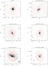 |
Fig. A.1. HST-ACS images (8″ × 8″ size) centered at the coordinates of some of our targets, as shown at the top of each image. North is up, east is left. As in Fig. A.3, NOEMA contours are shown in red, in case of CO detections. The archival HST image of A2219-1 is taken with the F850LP filter, while those of HLS sources are taken with the F818W filter. Small shifts ≤0.6 arcsec are applied to the images, consistent with GCS catalog uncertainties in the absolute astrometry used by HST. |
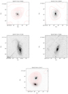 |
Fig. A.1. continued. |
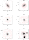 |
Fig. A.2. Subaru images (8″ × 8″ size), with the exception of A697-1 (12″ × 12″ size), centered at the coordinates of some of our targets, as shown at the top of each image. The i+-band is considered for all sources except for A963-1 and A963-1, for which the Ic-filter is used. The sources do not have available HST observations and are therefore not reported in Fig. A.1. North is up, east is left. As in Fig. A.3, NOEMA contours are shown in red. Small shifts ≤0.34 arcsec are applied to the images, consistent with the absolute Subaru astrometric uncertainties. |
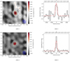 |
Fig. A.3. Left: clean intensity maps showing the CO detections obtained with NOEMA. Coordinates are reported as angular separations from the target sources. For each map, the velocity range considered corresponds to the velocity support associated with the corresponding CO emission line, see right panels. The solid and dashed contour levels are superimposed and correspond to positive and negative fluxes, starting from +2σ and −1σ levels, respectively. Consecutive levels correspond to an absolute increment of 1σ in significance. The dashed ellipses (bottom right) show the beam size. Right: spectrum (black solid line) obtained with NOEMA within an aperture corresponding to the beam size at the location of the detection, as reported in the left panels. The best fits, baseline subtracted, are reported (red dashed line). |
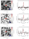 |
Fig. A.3. continued. |
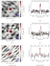 |
Fig. A.3. continued. |
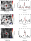 |
Fig. A.3. continued. |
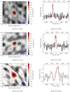 |
Fig. A.3. continued. |
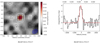 |
Fig. A.3. continued. |
All Tables
All Figures
|
Fig. 1. HST-ACS mosaic (F818W filter) of MACS J0717.5+3745. Our targets are highlighted as red dots. The solid blue circle has a radius equal to r200, while the solid orange contour represents the weak-lensing mass reconstruction by Jauzac et al. (2012) (at a 3σ level) showing the cluster and its associated large-scale filament extending in the southeast direction. |
| In the text | |
|
Fig. 2. Examples of FIR-to-UV MAGPHYS SED fits (solid black curve) for some of our targets. The galaxy IDs are indicated at the bottom of each panel. The photometric data points, corrected for Galactic extinction, are shown as red points. The solid blue curves show the SED fits in the absence of dust. Bottom panels: residuals. |
| In the text | |
|
Fig. 3. a: SFR vs.z and b: M⋆vs.z scatter plots. The green dotted line in panel a shows the empirical SFR values by Speagle et al. (2014) for MS field galaxies (SFRMS) with stellar mass log(M⋆/M⊙) = 10.6, which corresponds to the mean stellar mass for the LIRGs in our sample. c,d: molecular gas to stellar mass ratio as function of redshift; the two plots differ in terms of the adopted αCO, as shown at the bottom right of the panels. The green dotted lines show the empirical values found by Tacconi et al. (2018) for MS field galaxies with a stellar mass log(M⋆/M⊙) = 10.6. The color code for the data points is given in panels a,b. |
| In the text | |
|
Fig. 4. a: star formation rate as a function of stellar mass, the MS relation at different redshifts from Speagle et al. (2014) is shown as dotted green lines. b–d: SFR, molecular gas to stellar mass ratio, and depletion time, respectively, all normalized by the corresponding MS values (Speagle et al. 2014; Tacconi et al. 2018), as a function of the stellar mass. The color code for the data points is analogous to Fig. 3. Panels b–d: the horizontal dashed line refers to the MS value, that is, the y-axis value equal to unity, while the horizontal dotted lines show the range of y-axis values corresponding to MS galaxies. |
| In the text | |
|
Fig. 5. Star formation rate to SFRMS (left panel) and stellar mass (right panel), as a function of r/r200 of the LIRGs. Symbols are shown as in Fig. 3b. Blue, green, yellow, and red data points correspond to increasing SFR/SFRMS values, as illustrated in the color bar (left). Left panel: the horizontal dashed line refers to the MS value, while the horizontal dotted lines show the ±0.48 dex scatter corresponding to MS galaxies. |
| In the text | |
|
Fig. 6. Phase space diagram for all cluster galaxies in our sample. In the x-axis we plot the projected cluster centric radius, r, normalized to r200, while in the y-axis we plot the line-of-sight velocity, normalized to the cluster velocity dispersion σcluster. The dark and light gray areas show the range of virialized regions defined by Jaffé et al. (2015) for the clusters in our sample. |
| In the text | |
|
Fig. 7. Molecular gas to stellar mass ratio (left) and depletion time (right), normalized to the corresponding MS values, as a function of r/r200. The data points have different symbols and are color-coded according to the corresponding SFR/SFRMS, as in Fig. 6. In each panel, the horizontal dashed line refers to the MS value, while the horizontal dotted lines show the range of y-axis values corresponding to MS galaxies. |
| In the text | |
|
Fig. A.1. HST-ACS images (8″ × 8″ size) centered at the coordinates of some of our targets, as shown at the top of each image. North is up, east is left. As in Fig. A.3, NOEMA contours are shown in red, in case of CO detections. The archival HST image of A2219-1 is taken with the F850LP filter, while those of HLS sources are taken with the F818W filter. Small shifts ≤0.6 arcsec are applied to the images, consistent with GCS catalog uncertainties in the absolute astrometry used by HST. |
| In the text | |
|
Fig. A.1. continued. |
| In the text | |
|
Fig. A.2. Subaru images (8″ × 8″ size), with the exception of A697-1 (12″ × 12″ size), centered at the coordinates of some of our targets, as shown at the top of each image. The i+-band is considered for all sources except for A963-1 and A963-1, for which the Ic-filter is used. The sources do not have available HST observations and are therefore not reported in Fig. A.1. North is up, east is left. As in Fig. A.3, NOEMA contours are shown in red. Small shifts ≤0.34 arcsec are applied to the images, consistent with the absolute Subaru astrometric uncertainties. |
| In the text | |
|
Fig. A.3. Left: clean intensity maps showing the CO detections obtained with NOEMA. Coordinates are reported as angular separations from the target sources. For each map, the velocity range considered corresponds to the velocity support associated with the corresponding CO emission line, see right panels. The solid and dashed contour levels are superimposed and correspond to positive and negative fluxes, starting from +2σ and −1σ levels, respectively. Consecutive levels correspond to an absolute increment of 1σ in significance. The dashed ellipses (bottom right) show the beam size. Right: spectrum (black solid line) obtained with NOEMA within an aperture corresponding to the beam size at the location of the detection, as reported in the left panels. The best fits, baseline subtracted, are reported (red dashed line). |
| In the text | |
|
Fig. A.3. continued. |
| In the text | |
|
Fig. A.3. continued. |
| In the text | |
|
Fig. A.3. continued. |
| In the text | |
|
Fig. A.3. continued. |
| In the text | |
|
Fig. A.3. continued. |
| In the text | |
Current usage metrics show cumulative count of Article Views (full-text article views including HTML views, PDF and ePub downloads, according to the available data) and Abstracts Views on Vision4Press platform.
Data correspond to usage on the plateform after 2015. The current usage metrics is available 48-96 hours after online publication and is updated daily on week days.
Initial download of the metrics may take a while.