| Issue |
A&A
Volume 640, August 2020
|
|
|---|---|---|
| Article Number | A114 | |
| Number of page(s) | 11 | |
| Section | Interstellar and circumstellar matter | |
| DOI | https://doi.org/10.1051/0004-6361/201936661 | |
| Published online | 25 August 2020 | |
NH3 (1,1) hyperfine intensity anomalies in the Orion A molecular cloud
1
Xinjiang Astronomical Observatory, CAS 150, Science 1-Street Urumqi,
Xinjiang 830011,
PR China
e-mail: This email address is being protected from spambots. You need JavaScript enabled to view it.
2
Key Laboratory of Radio Astronomy, Chinese Academy of Sciences,
Urumqi 830011,
PR China
3
University of Chinese Academy of Sciences,
No.19(A) Yuquan Road, Shijingshan District,
Beijing
100049, PR China
4
Max-Planck-Institut für Radioastronomie,
Auf dem Hügel 69,
53121
Bonn, Germany
5
Astronomy Department, King Abdulaziz University,
PO Box 80203,
Jeddah 21589, Saudi Arabia
6
School of Astronomy and Space Science, Nanjing University,
163 Xianlin Avenue,
Nanjing 210023,
PR China
Received:
10
September
2019
Accepted:
16
June
2020
Abstract
Ammonia (NH3) inversion lines, with their numerous hyperfine components, are a common tracer used in studies of molecular clouds (MCs). In local thermodynamical equilibrium, the two inner satellite lines (ISLs) and the two outer satellite lines (OSLs) of the NH3(J, K) = (1,1) transition are each predicted to have equal intensities. However, hyperfine intensity anomalies (HIAs) are observed to be omnipresent in star formation regions, a characteristic which is still not fully understood. In addressing this issue, we find that the computation method of the HIA by the ratio of the peak intensities may have defects, especially when used to process the spectra with low-velocity dispersions. Therefore, we defined the integrated HIAs of the ISLs (HIAIS) and OSLs (HIAOS) by the ratio of their redshifted to blueshifted integrated intensities (unity implies no anomaly) and developed a procedure to calculate them. Based on this procedure, we present a systematic study of the integrated HIAs in the northern part of the Orion A MC. We find that integrated HIAIS and HIAOS are commonly present in the Orion A MC and no clear distinction is found at different locations of the MC. The medians of the integrated HIAIS and HIAOS are 0.921 ± 0.003 and 1.422 ± 0.009, respectively, which is consistent with the HIA core model and inconsistent with the collapse or expansion (CE) model. In the selection of those 170 positions, where both integrated HIAs deviate by more than 3σ from unity, most (166) are characterized by HIAIS < 1 and HIAOS > 1, which suggests that the HIA core model plays a more significant role than the CE model. The remaining four positions are consistent with the CE model. We compare the integrated HIAs with the para-NH3 column density (N(para-NH3)), kinetic temperature (TK), total velocity dispersion (σv), non-thermal velocity dispersion (σNT), and the total opacity of the NH3(J, K) = (1,1) line (τ0). The integrated HIAIS and HIAOS are almost independent of N(para-NH3). The integrated HIAIS decreases slightly from unity (no anomaly) to about 0.7 with increasing TK, σv, and σNT. The integrated HIAOS is independent of TK and reaches values close to unity with increasing σv and σNT. The integrated HIAIS is almost independent of τ0, while the integrated HIAOS rises with τ0, thus showing higher anomalies. These correlations cannot be fully explained by either the HIA core nor the CE model.
Key words: stars: formation / ISM: individual objects: Orion A molecular cloud / ISM: molecules / line: profiles / radio lines: ISM
© ESO 2020
1 Introduction
Ammonia (NH3) is a very important tracer in determining the density (e.g., Cheung et al. 1969), temperature (e.g., Ho et al. 1981), velocity (e.g., Goodman et al. 1993), and intrinsic line width (e.g., Barranco & Goodman 1998) of Molecular Clouds (MCs). Due to its high abundance (for the observed range, see Benson & Myers 1983; Mauersberger et al. 1987; Weiß et al. 2001), specific hyperfine structure and sensitivity to kinetic temperature (Ho & Townes 1983), NH3 inversion transitions are commonly used in studies related to star forming regions (SFRs), MCs, and nearby galaxies (e.g., Zhang et al. 1998; Henkel et al. 2005; Lu et al. 2014; Wu et al. 2018a). The ground state para NH3 (J, K) = (1,1) transition consists (due to electric quadrupole splitting) of five distinct components, namely, the main component (ΔF = 0) and four satellite components (ΔF = ±1), two on each side of the main component (Ho & Townes 1983). Weaker magnetic spin-spin interactions introduce a total of 18 hyperfine components within the profiles of the five quadrupole hyperfine components (see Fig. 1 in Rydbeck et al. 1977).
The two inner satellite lines (ISLs) and the two outer satellite lines (OSLs) are predicted to have equal intensities (26% for each ISL and 22% for each OSL with respect to the intensity of the main line under conditions of local thermodynamical equilibrium (LTE) and optically thin emission). This is used to model important parameters such as opacity, temperature, and column density (e.g., Ho & Townes 1983). However, it was found that the expectation of equal intensities of the ISLs and OSLs is not always valid. Matsakis et al. (1977) discovered a hyperfine intensity anomaly (HIA) in the case of absorption spectra towards the continuum background of DR21. Later, HIAs were found to be commonly present in MCs and SFRs (e.g., Stutzki et al. 1984; Longmore et al. 2007; Nishitani et al. 2012). More recently, Camarata et al. (2015) studied the HIA in a sample of 343 SFRs. They found that the HIA is ubiquitous in high-mass SFRs and that there is no clear correlation between the HIA and the temperature, line width, optical depth, or the stage of stellar evolution. However, the result may be affected by the computation method these authors have used to calculate the HIA (see Sect. 3). Therefore, the aim of this article is to quantify such uncertainties and to propose a better way to determine HIAs.
A compelling question asks what it is that causes HIAs. In analytical and numerical calculations, the HIA can be reproduced by non-LTE populations induced by trapping of selected hyperfine transitions in the rotational lines of NH3 connecting the (J, K) = (2,1) and (1,1) inversion doublets (e.g., Matsakis et al. 1977). An alternative scenario involves systematic motions, such as expansion and contraction (e.g., Park 2001).
If the former mechanism causes the HIA, the emitting cloud should be composed of several small cores with line widths of about 0.3–0.6 km s−1 (hereafter core model) since clouds with larger line widths would reshuffle the non-thermal populations (see Stutzki & Winnewisser 1985). The HIA is then expected to decrease with density, temperature, and line width (e.g., Camarata et al. 2015). The HIA of the ISLs (redshifted versus blueshifted component, HIAIS) can only be smaller than unity while the HIA of the OSLs (again redshifted versus blueshifted component, HIAOS) can only be larger than unity (e.g., Stutzki & Winnewisser 1985). Based on this mechanism, the HIA emitting clouds should be composed of many small (10−2 pc), high density (106 –107 cm−3) clumps of 0.3–1 M⊙ (e.g., Matsakis et al. 1977; Stutzki & Winnewisser 1985), which is further interpreted as being compatible with the “competitive accretion” model of high-mass star formation (e.g., Camarata et al. 2015).
In the latter case, (systematic) collapse or expansion, such as outflow, infall, or rotation in clouds, could lead to HIAs (hereafter, the CE model). Photons emitted from one hyperfine transition can be absorbed by another one due to systematic motions resulting in severe changes in the level populations of the NH3 (1,1) sub-levels. Expansion (contraction) can only strengthen the emission on the red (blue) side, while suppressing those on the other side (e.g., Park 2001). In principle, a cloud with collapsing and also expanding parts may lead to emission enhancements on different sides of the ISLs and OSLs, but such a situation may not be common (e.g., Matsakis et al. 1977). Based on this, the HIA is expected to be a tracer of systematic motions (e.g., Park 2001; Longmore et al. 2007). It is also expected to be strengthened as the ammonia column density increases since photon trapping processes are more efficient at larger optical depths (e.g., Park 2001). However, the HIA is still not fully understood. To date, we do not know why HIAs are so common in MCs and SFRs. There is not even any plausible clear correlation between the HIA and the physical properties of a cloud (Stutzki et al. 1984; Camarata et al. 2015).
A systematic observational study of HIAs could help us to address their origin. However, in previous observational studies, the authors focussed on single point observations towards separate star formation regions. Based on the latest extended and sensitive Green Bank Ammonia Survey1 (GAS; Friesen et al. 2017), we first provide a systematical study of the HIA in an extended and prominent cloud, the Orion A MC. With the criteria outlined in Sect. 3, we selected 1383 spectra in the northern part of the Orion A MC and studied the morphology and statistics of the HIA, as well as correlations between the HIA and several molecular gas parameters derived from these observations.
2 Data
The archival NH3 data we used to calculate the HIAs are derived from Green Bank Telescope (GBT) observations of the northern part of the Orion A MC, which is a part of the Green Bank Ammonia Survey (Friesen et al. 2017). The seven-beam K-Band Focal Plane Array (KFPA) was used as the front-end and the VErsatile GBT Astronomical Spectrometer (VEGAS) was used as the back-end. A spectral resolution of 5.7 kHz (0.07 km s−1 at 23.7 GHz) was derived under the VEGAS Mode 20. At the observed frequency, the GBT has a primary beam (FWHM) of about 32″ (0.065 pc). The data were observed in OTF mode and resampled with a sample step of about 10″. For more details, see Friesen et al. (2017).
The Orion A MC is the nearest and probably best studied MC that continues to produce both low- and high-mass stars (Bally 2008). At a distance of about 414 pc (Menten et al. 2007), it can be observed with good linear resolution. Meanwhile it is located about 15 degrees below the Galactic plane, leading to a less confused background than that typically encountered along the Galactic plane. The Orion A MC is the largest MC in the Orion complex (Wilson et al. 2005). The GBT observed region covers the northern compact ridge of the Orion A MC, which is an integral-shaped filamentary cloud (Bally et al. 1987; Johnstone & Bally 1999, 2006; Friesen et al. 2017; Wu et al. 2018a).
Baseline removal is critical when analysing NH3 data because any error in the slope of a baseline may lead to false HIAs. In order to minimize this problem, we only used linear polynomials to remove the baselines and all of these spectra selected have flat and gently varying baselines which can be well-fitted by the linear polynomials. The large threshold of the signal-to-noise ratio (S/N) we used (see below) will likely further reduce any baseline related effects.
Matplotlib2 (Hunter 2007), lmft3 (Newville et al. 2014), scipy4, ApLpy5 (Jones et al. 2001), montage6 and GILDAS7 software packages were used in the data reduction and display.
3 Results
As we have mentioned in the introduction, there is a total of 18 hyperfine components within the profiles of the five quadrupole hyperfine components of the (J, K) = (1,1) line.The ISLs (OSLs) contain three (two) hyperfine components with different velocity separations (see the cyan vertical lines in Fig. A.1 and also Rydbeck et al. 1977). Assuming all the 18 hyperfine components are optically thin and have Gaussian profiles with the same velocity dispersion, as we may expect, the ISLs (or OSLs) which are the combination of Gaussian spectra of three (or two) hyperfine components with different offsets should have different line widths and peak intensities. To the contrary, the integrated intensities (flux) of the ISLs (orOSLs) over specific integrated velocity ranges should show equal values (see Fig. A.2). Therefore, the HIA calculated with the peak intensities from single Gaussian fittings (hereafter, peak HIA; e.g., Longmore et al. 2007; Camarata et al. 2015) does not reflect the real anomaly. The HIA calculated from integrated intensities (hereafter integrated HIA) provides a less biased view (see Appendix A for details).
Therefore, to calculate the HIA in this paper, we adopt
 (1)
(1)
and
 (2)
(2)
where FRISL and FBISL are the integrated intensities of the red- and blueshifted sides of the ISLs, respectively. Accordingly FROSL and FBOSL are the integrated intensities of the red- and blueshifted sides of the OSLs. The integrated ranges are all set to ± 2 × ΔV of each of the 18 hyperfine components, which is explained in Appendix B.
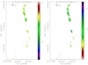 |
Fig. 1 Integrated hyperfine intensity anomalies of the inner satellite lines (left panel) and the outer satellite lines (right panel) derived from 1383 spectra with an S/N larger than 15 in the Integral-Shaped Filament (ISF) of the Orion A molecular cloud. The blue cross in each panel illustrates the location of the Orion Kleinmann-Low Nebula (RA 05:35:14.16 Dec -05:22:21.5 J2000). |
3.1 Distributions of integrated HIAs in the Orion MC
Based on our procedure (Appendix B), we first excluded spectra with an S/N less than 15. We further excluded the spectra with velocity dispersions larger than 1.0 km s−1 (35 spectra mostly located around the Kleinmann-Low (KL) Nebula in OMC 1, RA 05:35:14.16 Dec −05:22:21.5 J2000). In cases where the velocity dispersion is larger than 1.0 km s−1, the main line and ISLs start to substantially overlap. Spectra with more than one velocity component were also discarded. Finally, 1383 spectra are selected to calculate the HIAs. The total optical depths of NH3 (1,1) (τ0, see Appendix B) of the selected spectra range from 0.12 to 2.98 and 89% of them are smaller than unity. This means for all of theselected spectra that the individual hyperfine components of the four satellite lines and even the blended emission of each inner and outer satellite group of hyperfine components is optically thin (see Table A.1, where relative intensities are given, normalized to unity). Figure 1 presents the distributions of the integrated HIAs calculated from the GBT data with our procedure. The left panel displays the integrated HIAIS and the right panel displays the integrated HIAOS. With the threshold of the S/N larger than 15, the majority of the available pixels are distributed north of the Kleinman-Low nebula and only a small number of the pixels are scattered along the southern part of the filamentary MC.
Firstly, we can see in the two panels (for the statistical results, see Sect. 3.2) that integrated HIAIS and HIAOS are commonly present in the Orion A MC. Secondly, there is no clear trend of the integrated HIAs along the MC. For example, there is no clear distinction between the integrated HIAs of the cloud around the KL Nebula and Trapezium cluster (i.e. the OMC1; Orion Cloud 1; Wiseman & Ho 1996), the more quiescent northern part of the cloud (OMC 2,3; Johnstone & Bally 1999; Li et al. 2013), and the more diffuse southern part of the cloud (OMC 4, 5; Johnstone & Bally 2006). Finally, the integrated HIAOS is distributed in a wider range than the integrated HIAIS.
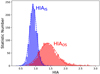 |
Fig. 2 Histograms of the integrated hyperfine intensity anomalies of the inner satellite lines (the blue histogram) and the outer satellite lines (the red histogram) of the spectra with an S/N larger than 15. The dashed blue and red lines represent the fitted results by assuming that they are subject to Gaussian distributions. |
Statistical results of the integrated hyperfine intensity anomaly of the inner satellite lines and outer satellite lines.
3.2 Statistics of the integrated HIAs
We present the statistical results of the integrated HIAs in Fig. 2 and Table 1. We can see, as already outlined in Sect. 3.1, that (1) most of the ratios do not equal unity and (2) the integrated HIAIS is distributed in a narrower range than the HIAOS. The medians of the integrated HIAIS and HIAOS are 0.921 ± 0.003 and 1.422 ± 0.009, respectively; the errors representing standard deviations of the mean. The statistical results can be compared with those of Camarata et al. (2015) in a sample of 334 high-mass SFRs (0.889 ± 0.004 and 1.232 ± 0.006), which are further discussed in Appendix A.2. (3) The integrated HIAIS and HIAOS are distributed on both sides of unity.
As outlined in the introduction, the HIA core model predicts that the HIAIS can only be smaller than unity and the HIAOS can only be larger than unity (e.g., Stutzki & Winnewisser 1985; Camarata et al. 2015). To the contrary, the CE model predicts the HIAIS and HIAOS should be simultaneously larger and smaller than unity (e.g., Park 2001). We can see in Fig. 2 that the overall “inverse” distributions relative to unity (0.921 ± 0.003 and 1.422 ± 0.009, respectively) of the integrated HIAIS and HIAOS are consistent with the HIA core model (e.g., Matsakis et al. 1977; Stutzki & Winnewisser 1985) and inconsistent with the CE model (e.g., Park 2001), as also suggested by Camarata et al. (2015). However, as we can see in Fig. 2, there are still some ratios of the ISLs which are larger than unity and some ratios of the OSLs which are smaller than unity.
To further investigate the distributions of the integrated HIAs, we present a direct plot of the integrated HIAIS and HIAOS in Fig. 3. The panel is divided into four quarters, which are labelled as I, II, III, and IV in Fig. 3 by the two dashed grey lines (HIAIS = 1, HIAOS = 1). The blue- and red points denote positions, where both HIAIS and HIAOS deviate by more than 1 and 3σ from unity. The black points highlight positions where only one of the HIAs deviates by more than 1σ from unity and the green points indicate locations, where both the HIAIS and HIAOS are within 1σ from unity. Again, we can see that most of the integrated HIAs do not equal unity.
The core model predicts that all points should be in the second quarter (HIAIS<1, HIAOS>1), while the CE model predicts that the points should either lie in the first quarter (HIAIS>1, HIAOS>1) or the third quarter (HIAIS<1, HIAOS<1). We can see in the figure that most of the points are distributed in the upper two quarters (HIAOS>1), especially the second quarter, but there are also a handful of points located in the third and forth quarters. As suggested by, for example, Stutzki et al. (1984), a deviation from unity by more than 3σ clearly shows an anomalous emission. Taking the HIA uncertainties (the uncertainties are illustrated in Appendix B) into consideration, we have a total of 170 points, indicated by a red color, whose integrated HIAIS and HIAOS deviate from unity by more than their 3σ uncertainties. We can see in Fig. 3 that 166 red points are located in the second quarter and 4 red points in the first quarter. These statistical properties suggest that the HIA core model is playing the dominant role, while only 4 out of 170 points support the CE model. In this context, it is interesting to note that we find all these four positions in the first quarter of the diagramand none in the third quarter. This is consistent, following the CE model (Sect. 1), with the expansion of the molecular gas.
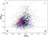 |
Fig. 3 Distribution of the integrated hyperfine intensity anomalies of the inner (HIAIS) and outer (HIAOS) satellite lines. The red (blue) points illustrate positions, where both the HIAIS and HIAOS values deviate by more than 3σ (1σ) from unity. Black points denote positions, where either the HIAIS or the HIAOS is located within 1σ of unity, while the green points show positions, where both the HIAIS and HIAOS are within 1σ of unity. Grey dashed vertical and horizontal lines subdivide the panel into regions with HIAIS >1 (labelled I for HIAOS>1 and IV for HIAOS<1) and HIAIS<1 (labeled II for HIAOS>1 and III for HIAOS<1). |
4 Discussion
We compare the integrated HIAs with the para-NH3 column density (N(para-NH3)), kinetic temperature (TK), intrinsic velocity dispersion (σv), non-thermaldispersion (σNT), and the total opacity of NH3) (1,1) (τ0), which are all derived from NH3 (1,1) and (2,2) observations. σv and τ0 are derived from our procedure (Appendix B). N(para-NH3) and TK are taken from Friesen et al. (2017). The routines to calculate these parameters are also illustrated there. σNT is calculated by  , where
  = 17, mH = 1.674 × 10⁻²⁴ g, k is the Boltzmann constant, and TK is the kinetic temperaturecalculated from NH3 (1,1) and (2,2). We summarise all the comparisons in Fig. 4. The linear regression results are also presented in each panel (red and blue lines) and in Table 2. In all the regressions, the correlation coefficient takes a range of values from −1 (a perfect negative correlation) to +1 (a perfect positive correlation). A correlation coefficient of zero indicates no relationship between the two variables being compared.
Firstly, we can see from panel a in Fig. 4 that the integrated HIAs are almost independent of N(para-NH3) (the correlation coefficients of the integrated HIAIS and HIAOS are −0.029 and 0.027 respectively). Then we can see from panel b in Fig. 4 that the integrated HIAIS decreases from unity to about 0.7, indicating higher anomalies, with increasing temperature. However, the correlation is weak, with a correlation coefficient of −0.35. On the other hand, the integrated HIAOS seems to show a decrease at the high temperature end (TK > 40 K). Probably due to the large dispersion of the integrated HIAOS, a clear correlation between the integrated HIAOS and TK is not present (the correlation coefficient is −0.05). We can also see from panels c and d in Fig. 4 that the integrated HIAs decrease slightly with increasing σv and σNT, but again with low correlation coefficients (see Table 2). The integrated HIAIS deviates more and more from unity, while the HIAOS moves closer and closer to unity with increasing σv or σNT. It should be noted that TK, σNT, and σv are not independent of one another. Thus, the correlations between the integrated HIAs, TK, σv, and σNT show similarities. Finally, we can see from panel (e) in Fig. 4 that the integrated HIAIS appears to be independent of τ0. On the contrary, the integrated HIAOS appears to rise with τ0 and shows higher anomalies with increasing τ0.
We should note that the correlation coefficients are all small. The maximal correlation coefficient of −0.35 is found between the integrated HIAIS and TK. Overall, the correlations between the integrated HIAs and potentially related parameters (Fig. 4) are weaker than what the models predict. This may partially be due to the very large dispersion in the HIAOS. Nevertheless, the current results are not fully explained, neither by the HIA core model nor by the CE model. For example, the HIA core model cannot explain that the integrated HIAIS deviates more and more from unity with increasing TK, σv, and σNT. The HIA core model requires subcores with line widths of 0.3–0.6 km s−1 (Sect. 1). The strength of the anomaly is then expected to decrease with increasing temperature and line width. The HIA CE model cannot explain the integrated HIAIS and HIAOS have opposite trends relative to unity with increasing σv and σNT. The integrated HIAs are independent of N(para-NH3), while the CE core model predicts that the integrated HIAIS and HIAOS are strengthened when the ammonia column density increases (e.g., Park 2001). Finally, the correlations of the integrated HIAs with σNT suggest that non-thermal motions (e.g., turbulence) might also have contributions to the HIAs as suggested by Camarata et al. (2015).
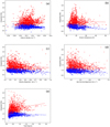 |
Fig. 4 Comparisons of the integrated hyperfine intensity anomalies (inner satellites: blue dots; outer satellites: red dots) with the para-NH3 column density (a), kinetic temperature (b), velocity dispersion (c), non-thermal velocity dispersion (d), and total optical depth of NH3 (1,1) (e) all derived from the GBT NH3 observations(Friesen et al. 2017). |
Statistical results of the integrated hyperfine intensity anomalies (HIAs) of the inner satellite lines (ISLs) and outer satellite lines (OSLs) as function of para-ammonia column density, kinetic temperature, velocity dispersion, the turbulent part of the velocity dispersion, and the total opacity of NH3 (1,1).
5 Conclusions
- 1.
Through our simulations (Fig. A.2) and GBT observations (Fig. A.6), we demonstrate that the integrated HIAs calculated from the integrated intensities should be less biased than the peak HIAs calculated from the peak intensities, due to the different separations of the 18 hyperfine components within the inner and outer satellite lines (ISLs and OSLs) and their asymmetric profiles.
- 2.
We developed a procedure (Appendix B) to fit the NH3 (1,1) profiles and to calculate the integrated and peak HIAs. Based on this procedure, we first present a study of the HIAs in the Orion A molecular cloud (MC). We do not find clear differences or trends in the integrated HIAIS and HIAOS along the filamentary MC.
- 3.
The medians of the statistical results of the integrated HIAIS and HIAOS (defined by the integrated intensity ratios of their redshifted to blueshifted components) have “inverse” values relative to unity, that is, 0.921 ± 0.003 and 1.42 ± 0.009, respectively, which is consistent with the HIA core model and inconsistent with the CE model. Accounting for the 3-σ uncertainties of the individual positions, most (166) of the integrated HIAs are characterised by HIAIS<1 and HIAOS>1, which is again consistent with the HIA core model. However, there are also four positions with HIAIS>1 and HIAOS>1, which supports the CE model, suggesting expanding gas. These results indicate that the HIA core model plays a more significant role than the CE model.
- 4.
We compared the integrated HIAs with the para-NH3 column density (N(para-NH3)), kinetic temperature (TK), velocity dispersion (σv), non-thermal velocity dispersion (σNT), and NH3 total opacity (τ0). The integrated HIAs are within the uncertainties independent of N(para-NH3). The integrated HIAIS deviates more and more from unity with increasing temperature while the integrated HIAOS is almostindependent of TK. The integrated HIAs all decrease with increasing σv and σNT. With increasing σv and σNT, the integrated HIAIS is getting below unity and thus more anomalous, while the integrated HIAOS decreases to unity (no anomaly). The integrated HIAIS appears to be independent of τ0, but the integrated HIAOS appears to rise with τ0 and shows higher anomalies with increasing τ0. Neither the HIA core model nor the CE model can explain all these results.
Overall, we find that the HIA core model, related to trapping in some hyperfine level transitions, plays a more significant role. Nevertheless, the correlation results are not fully explained, either by the HIA core model nor by the CE model, based on the assumption of radial motions inside the studied clouds.
Acknowledgements
We would like to thank the anonymous referee for the useful suggestions that improved this study. This work was funded by the National Nature Science foundation of China under grant 11433008 and the CAS “Light of West China” Program under grant Nos. 2018-XBQNXZ-B-024, and partly supported by the National Natural Science foundation of China under grant 11603063, 11973076, 11703074, and 11703073. G. W. acknowledges the support from Youth Innovation Promotion Association CAS. This research has made use of NASA’s Astrophysics Data System Bibliographic Services. This research made use of Montage. It is funded by the National Science Foundation under Grant Number ACI-1440620, and was previously funded by the National Aeronautics and Space Administration’s Earth Science Technology Office, Computation Technologies Project, under Cooperative Agreement Number NCC5-626 between NASA and the California Institute of Technology.
Appendix A The computation method: peak or integrated intensity ratios?
A.1 Comparison with the simulated spectra
In order to test the expectation that the integrated HIA is less biased than the peak HIA (see Sect. 3) and to simulate the results we could derive from the observed data, we created a simulated spectrum with a specific velocity dispersion by assuming all the 18 hyperfine components have Gaussian profiles and the same velocity dispersion (e.g., Rosolowsky et al. 2008; Mangum & Shirley 2015). The simulated spectrum can then be described by
![Mathematical equation: \begin{equation*} S(V) = \sum^{18}_{i=1} R_{\textrm{hfs}}[i] \times A_{0} \times e^{- (V - V_{0} - V_{\textrm{hfs}}[i])^{2} /(2*\sigma_{\textrm{V}}^{2})}, \end{equation*}](/articles/aa/full_html/2020/08/aa36661-19/aa36661-19-eq5.png) (A.1)
(A.1)
where S(V) is the simulated spectrum combining all the 18 hyperfine components, Rhfs[i] and Vhfs[i] are the relative intensities of individual features under the conditions of LTE and optically thin emission (see Table A.1), and the relative velocities, which are given in Rydbeck et al. (1977) (see Table A.1). A0 and V0 represent the arbitrary amplitude and velocity offset of the combined spectrum, which are set to 0.5 and zero, respectively. σV denotes the velocity dispersion for each of the 18 hyperfine components.
Predicted relative intensities, frequency and velocity separations of the 18 hyperfine components of NH3 (1,1).
We present an example of a simulated spectrum with a velocity dispersion of 0.5 km s−1 in Fig. A.1. The black thick line shows the combined NH3 (1,1) spectrum. The thick blue vertical lines below the zero level show the integrated ranges used to calculate the integrated HIAIS and HIAOS. The orange vertical lines above the zero level indicate the ranges of the sub-spectra used to fit the inner and outer satellite lines with single Gaussian functions. The red lines present the single Gaussian fitting results. The cyan vertical lines present the 18 hyperfine components given in Rydbeck et al. (1977). The lengths and the separations of these lines (see Table A.1) represent their expected intensities and velocity separations.
We then created 1000 simulated spectra with linearly spaced velocity dispersions from 0.1 to 1.2 km s−1 to further study the relationship between the peak and integrated HIAs against the velocity dispersion. Applying the procedure which is described in Appendix B, we fitted these spectra and derived the peak and integrated HIAs, respectively, which are presented in Fig. A.2. The red and blue lines show the derived integrated HIAIS and HIAOS. The green and cyan lines present the derived peak HIAIS and HIAOS. Two grey dashed lines indicate the velocity dispersion range of the GBT data we used (0.14–1.0 km s−1). Oscillations of the blue line (the integrated HIAIS) are present at the large velocity dispersion end (≳1.0 km s−1), because the main line and ISLs start to overlap and the main line has an asymmetric profile. At the low velocity dispersion end (<0.1 km s−1) there are fluctuations of all the HIAs. Fluctuations of the peak HIAs arise at low velocity dispersions because the spectra develop multi-peaks, which reduce the Gaussian fitting precision. Fluctuations of the integrated HIAs occur because the velocity ranges at these dispersions only cover a relatively small part of the ISLs or OSLs. However, within the velocity dispersion range of the observed data we used (dashed vertical lines in Fig. A.2), these effects can be ignored.
We should note that all the 18 hyperfine components have infinite line wings. Obviously, this also holds for the combined five distinct quadrupole hyperfine components of the NH3 (1,1) line. The derived integrated HIAs are approximately one, but are not equal to unity since the integrated range cannot cover all the line wings. For example, for velocity dispersions from 0.14 to 1.0 km s−1 (the velocity dispersion range of the observed data we used), the maximal deviations from unity are 0.00398 and 0.00323 for the integrated HIAIS and HIAOS, respectively.Compared with the spectral noise of the observed data, these deviations can be neglected.
As we can see in Fig. A.2, the integrated HIAIS and HIAOS are very close to unity. However, clear dichotomies are present between the peak HIAs and unity. Therefore, with the theoretically predicted intensities and the velocity separations of all the 18 hyperfine components, the previously used method, using the peak intensities to calculate the HIAs, can “produce” anomalies especially at the low velocity dispersion end. Peak and integrated HIAs derived from the observed data are compared in Appendix A.2.
A.2 Comparison with the observed spectra
Complementing Fig. A.1, we also present an example of an observed NH3 (1,1) spectrum with a fitted velocity dispersion of 0.495 km s−1 in Fig. A.3 using the procedure outlined in Appendix B. The black polyline shows the observed NH3 (1,1) spectrum. The thick blue vertical lines below the zero level indicate the integrated ranges used to calculate the integrated HIAIS and HIAOS. The orange vertical lines indicate the ranges of the sub-spectra used to fit the inner and outer satellite lines with single Gaussian functions. The green line presents the result of the 18 hyperfine components fitting. The red lines illustrate the single Gaussian fitting results. The cyan vertical lines show the 18 hyperfine components given in Table A.1. The lengths and separations of these lines represent their predicted intensities and velocity separations. Because the fitting methods are different and the satellite lines have intensity anomalies and asymmetric profiles, there are slight differences between the green (18 hyperfine components fitting) and red (single Gaussian fitting) lines.
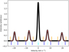 |
Fig. A.1 Simulated optically thin NH3 (1,1) spectrum under conditions of local thermodynamical equilibrium with a velocity dispersion of 0.5 km s−1. The black line presents the simulated spectrum. The thick orange vertical lines above the zero level show the ranges of the sub-spectra used to fit the inner and outer satellite lines with single Gaussian functions. The thick blue vertical lines below the zero level indicate the integrated ranges used to calculate the integrated hyperfine intensity anomalies of the inner and outer satellite lines. The red lines show the single Gaussian fitting results. The cyan vertical lines below the zero level present the 18 individual hyperfine components listed in Table A.1. The lengths and separations of the lines denote their predicted intensities and velocity separations. |
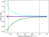 |
Fig. A.2 Peak and integrated hyperfine intensity anomalies derived from the simulated spectra against the velocity dispersion. The blue and red lines present the integrated hyperfine intensity anomalies of the inner and outer satellite lines, respectively. The green and cyan lines present the peak hyperfine intensity anomalies of the inner and outer satellite lines, respectively. Two grey dashed lines indicate the velocity dispersion range of the GBT data we used. |
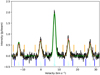 |
Fig. A.3 Example of an observed NH3 (1,1) spectrum with a fitted velocity dispersion of 0.495 km s−1. The black line presents the observed spectrum. The green line presents the result of the 18 hyperfine components fitting. The thick orange vertical lines show the ranges of the sub-spectra used to fit the inner and outer satellite lines with single Gaussian functions. The thick blue vertical lines below the zero level show the ranges used to calculate the integrated hyperfine intensity anomalies of the inner and outer satellite lines. The red lines indicate the single Gaussian fitting results. The cyan vertical lines below the zero level present the 18 hyperfine individual components listed Table A.1. The lengths and separations of these cyan lines denote their expected intensities and velocity separations. |
In Fig. A.4, direct comparisons of the peak and integrated HIAs are presented. The peak HIAIS and integrated HIAIS are shown in the left panel. The peak HIAOS and integrated HIAOS are presented in the right panel. We can see in this figure that the peak HIAs are still roughly proportional to the integrated HIAs, especially the HIAOS. In Fig. A.5, the peak (red dots) and integrated (blue dots) HIAs are plotted against the velocity dispersions of ISLs (left panel) and OSLs (right panel). We can see that from large to small velocity dispersions, the peak HIAs and the integrated HIAs are gradually separated (see also Fig. A.2). However, the differences between the peak and integrated HIAs due to computation methods are contaminated by real intensity anomalies and spectral noise.
In order to clearly demonstrate the similarities and differences between the HIAs derived from the observations and simulations (Appendix A.1), we provide the subtraction of the peak and integrated HIAs derived from the observed data (red and blue dots) against their velocity dispersions in Fig. A.6. We also present the subtraction of the peak and integrated HIAs of the simulated spectra against their velocity dispersions as red and blue lines in Fig. A.6. We can see that the derived subtraction of the HIAs from the observed data shows the same trend as the subtraction of the HIAs from the simulations (Fig. A.2), that is, the deviations of the peak and integrated HIAs are getting larger and larger with decreasing velocity dispersion. Nevertheless, the differences between the observed peak and integrated HIAOS (red dots) are slightly smaller than the simulated ones. From the simulations and observations, the peak and integrated HIAs show the same dichotomies. Due to our simulations (see Fig. A.2), we know that the integrated HIAs should be more objective than the peak HIAs, especially dealing with spectra with low velocity dispersions, for example, spectra from quiescent clouds.
According to our results the commonly used definition of the HIA, i.e. the peak HIA (e.g., Longmore et al. 2007; Camarata et al. 2015), might be misleading. Nevertheless, the peak HIAs are still roughly proportional to the integrated HIAs. Meanwhile, most of the sample in Camarata et al. (2015) are high-mass star formation regions, that means the spectra in that sample have considerablevelocity dispersions (see their Fig. 3). In such objects, the difference between the peak and integrated HIAs is generally small. That is why the overall statistical results of our integrated HIAs are similar to the results of Camarata et al. (2015).
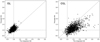 |
Fig. A.4 Peak hyperfine intensity anomalies against the integrated hyperfine intensity anomalies of the inner satellite lines (left panel) and outer satellite lines (right panel). |
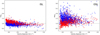 |
Fig. A.5 Peak (red) and integrated (blue) hyperfine intensity anomalies of the inner satellite lines (left panel) and outer satellite lines (right panel) against the velocity dispersion. |
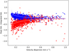 |
Fig. A.6 Subtraction of the peak and the integrated hyperfine intensity anomalies of the inner satellite lines (blue dots) and outer satellite lines (red dots) against the velocity dispersion. The blue and red lines denote the subtraction of the peak and integrated hyperfine intensity anomalies as obtained from the simulations presented in Fig. A.2. |
Appendix B The HIA procedure
In order to quantitatively investigate the integrated HIAs within the Orion A MC, we developed an HIA procedure to fit the NH3 (1,1) spectra and calculate the integrated and also the peak HIAs by the following steps:
- 1.
Extract the spectra with a single velocity component and an S/N larger than 15. The methods are illustrated in Wu et al. (2018b), that is, (1) the integrated intensity over the main line, that is, the central group of hyperfine components, must be larger than 15 times the noise (the spectral RMS noise times the square root of the number of channels covering the main line); (2) within the main line, there must be a minimum of two adjacent spectral channels also showing emission larger than 15 times their spectral RMS noise.
- 2.
We used the combined 18 Gaussian functions with the fixed relative amplitudes and velocity separations listed in Table A.1 to fit the observed or simulated NH3 (1,1) spectra. The observed data are fitted using optical depth as a function of velocity over the spectral band as in Eq. (B.1),
 (B.1)
(B.1)The optical depth of each hyperfine component is assumed to have a Gaussian profile and to be proportional to their predicted intensities in case of LTE (e.g., Friesen et al. 2009; Estalella 2017),
![Mathematical equation: \begin{equation*}\tau(V) = \tau_{0} \sum^{18}_{i=1} R_{\textrm{hfs}}(i) \times e^{-(V - V_{0} - V_{\textrm{hfs}}[i])^{2} /(2 \times \sigma_{\textrm{V}}^{2})}.\vspace*{-3pt} \end{equation*}](/articles/aa/full_html/2020/08/aa36661-19/aa36661-19-eq7.png) (B.2)
(B.2)The free parameters are the amplitude and velocity offset of the combined spectrum A0 and V0, the intrinsicvelocity dispersion (Barranco & Goodman 1998) of each of the 18 hyperfine components σV, and the total optical depth of NH3(1,1), τ0. Rhfs and Vhfs denote the predicted relative intensities in the optically thin case and velocity offsets of the 18 hyperfine components (see Table A.1).
- 3.
Based on the fitted velocity and the intrinsic velocity dispersion derived in step 2, we define the integrated velocity ranges as given in equation B.3 (thick blue vertical lines below the zero level in Figs. A.1 and A.3). These are used to calculate the integrated HIAs. For the four sub-components we use equation B.4 (thick orange vertical lines in Figs. A.1 and A.3) to fit the ISLs and OSLs with single Gaussian functions to obtain the peak HIAs. Here we applied two factors, fint and fpeak with
 (B.3)
(B.3)and
 (B.4)
(B.4)The hyperfine component intensity weighted velocity of the satellite is Vs = ∑iRhfs[i] × Vhfs[i]∕∑iRhfs[i] which is also given in Table 2. ∑i indicates that the summation is only for the two or three hyperfine components within each of the satellite lines. The FWHM line width
 . V0 represents the fitted velocity offset of the combined spectrum, σV represents the fitted velocity dispersion of each of the 18 hyperfine components. V0 and σV are all derived in step 2. The factor fpeak (Eq. (B.4)) is set to 2.5. The factor fint (Eq. (B.3)) is set to 2. This is because in our simulations, this choice largely restrains fluctuations and oscillations (see Sect. A.1) in the velocity dispersion range of 0.14–1.0 km s−1 (the range of the considered velocity dispersions). The velocity range considered for the derivation of the integrated HIA has been chosen to be slightly narrower than the one for the peak HIA to minimise the influence of noise in the calculation of integrated HIA values (see Eq. (B.5)).
 - 4.
For the integrated HIAs, we calculate the integrated intensities and the integrated HIAIS and HIAOS. For the peak HIAs, we fit each of the four satellite lines (sub-spectra) with a single Gaussian function and calculate the peak HIAIS and HIAOS. We should note that this peak HIA calculation method is the same as that used in for example, Stutzki et al. (1984), Longmore et al. (2007), and Camarata et al. (2015).
- 5.
The standard deviations of the integrated and peak HIAs (σint, σpeak) are assigned by
 (B.5)
(B.5)
 (B.6)
(B.6)where, HIApeak and HIAint are peak and integrated HIAs. Nc is the channel number within the integrated range. σhfs is the standard deviation of the 18 hyperfine components fitting (step 2). Fred and Fblue are the integrated intensities of the redshifted and blueshifted sides of the ISLs and OSLs. σpeak,red and σpeak,blue are the standard deviations of the single Gaussian fittings (step 4) of the redshifted and blueshifted sides of the ISLs or OSLs, respectively. Pred and Pblue are the fitted peaks of the blueshifted and redshifted sides of the ISLs or OSLs, respectively.
References
- Bally, J. 2008, Handbook of Star Forming Regions (USA: Astronomical Society of the Pacific), 4, 459 [Google Scholar]
- Bally, J., Langer, W. D., Stark, A. A., & Wilson, R. W. 1987, ApJ, 312, L45 [NASA ADS] [CrossRef] [Google Scholar]
- Barranco, J. A., & Goodman, A. A. 1998, ApJ, 504, 207 [NASA ADS] [CrossRef] [Google Scholar]
- Benson, P. J., & Myers, P. C. 1983, ApJ, 270, 589 [NASA ADS] [CrossRef] [Google Scholar]
- Camarata, M. A., Jackson, J. M., & Chambers, E. 2015, ApJ, 806, 74 [CrossRef] [Google Scholar]
- Cheung, A. C., Rank, D. M., Townes, C. H., Knowles, S. H., & Sullivan, W. T., III 1969, ApJ, 157, L13 [NASA ADS] [CrossRef] [Google Scholar]
- Estalella, R. 2017, PASP, 129, 025003 [NASA ADS] [CrossRef] [Google Scholar]
- Friesen, R. K., Di Francesco, J., Shirley, Y. L., et al. 2009, ApJ, 697, 1457 [NASA ADS] [CrossRef] [Google Scholar]
- Friesen, R. K., Pineda, J. E., co-PIs, et al. 2017, ApJ, 843, 63 [NASA ADS] [CrossRef] [Google Scholar]
- Goodman, A. A., Benson, P. J., Fuller, G. A., & Myers, P. C. 1993, ApJ, 406, 528 [NASA ADS] [CrossRef] [Google Scholar]
- Henkel, C., Jethava, N., Kraus, A., et al. 2005, A&A, 440, 893 [NASA ADS] [CrossRef] [EDP Sciences] [Google Scholar]
- Ho, P. T. P., & Townes, C. H. 1983, ARA&A, 21, 239 [NASA ADS] [CrossRef] [Google Scholar]
- Ho, P. T. P., Martin, R. N., & Barrett, A. H. 1981, ApJ, 246, 761 [CrossRef] [Google Scholar]
- Hunter, J. D. 2007, Comput. Sci. Eng., 9, 90 [NASA ADS] [CrossRef] [Google Scholar]
- Jones, E., Oliphant, E., Peterson, P., et al. SciPy: Open Source Scientific Tools for Python [Google Scholar]
- Johnstone, D., & Bally, J. 1999, ApJ, 510, L49 [NASA ADS] [CrossRef] [Google Scholar]
- Johnstone, D., & Bally, J. 2006, ApJ, 653, 383 [NASA ADS] [CrossRef] [Google Scholar]
- Li, D., Kauffmann, J., Zhang, Q., & Chen, W. 2013, ApJ, 768, L5 [NASA ADS] [CrossRef] [Google Scholar]
- Longmore, S. N., Burton, M. G., Barnes, P. J., et al. 2007, MNRAS, 379, 535 [NASA ADS] [CrossRef] [Google Scholar]
- Lu, X., Zhang, Q., Liu, H. B., Wang, J., & Gu, Q. 2014, ApJ, 790, 84 [NASA ADS] [CrossRef] [Google Scholar]
- Mangum, J. G., & Shirley, Y. L. 2015, PASP, 127, 266 [Google Scholar]
- Matsakis, D. N., Brandshaft, D., Chui, M. F., et al. 1977, ApJ, 214, L67 [NASA ADS] [CrossRef] [Google Scholar]
- Mauersberger, R., Henkel, C., & Wilson, T. L. 1987, A&A, 173, 352 [NASA ADS] [Google Scholar]
- Menten, K. M., Reid, M. J., Forbrich, J., & Brunthaler, A. 2007, A&A, 474, 515 [NASA ADS] [CrossRef] [EDP Sciences] [Google Scholar]
- Newville, M., Stensitzki, T., Allen, D. B., & Ingargiola, A. 2014, https://doi.org/10.5281/zenodo.11813 [Google Scholar]
- Nishitani, H., Sorai, K., Habe, A., et al. 2012, PASJ, 64, 30 [CrossRef] [Google Scholar]
- Ott, S. 2010, ASP Conf. Ser., 434, 139 [Google Scholar]
- Park, Y.-S. 2001, A&A, 376, 348 [NASA ADS] [CrossRef] [EDP Sciences] [Google Scholar]
- Rosolowsky, E. W., Pineda, J. E., Foster, J. B., et al. 2008, ApJS, 175, 509 [NASA ADS] [CrossRef] [Google Scholar]
- Rydbeck, O. E. H., Sume, A., Hjalmarson, A., et al. 1977, ApJ, 215, L35 [NASA ADS] [CrossRef] [Google Scholar]
- Stutzki, J., & Winnewisser, G. 1985, A&A, 144, 13 [NASA ADS] [Google Scholar]
- Stutzki, J., Jackson, J. M., Olberg, M., Barrett, A. H., & Winnewisser, G. 1984, A&A, 139, 258 [Google Scholar]
- Stutz, A. M., & Kainulainen, J. 2015, A&A, 577, L6 [NASA ADS] [CrossRef] [EDP Sciences] [Google Scholar]
- Thaddeus, P., Krisher, L. C., & Loubser, J. H. N. 1964, J. Chem. Phys., 40, 257 [NASA ADS] [CrossRef] [Google Scholar]
- Wilson, B. A., Dame, T. M., Masheder, M. R. W., & Thaddeus, P. 2005, A&A, 430, 523 [NASA ADS] [CrossRef] [EDP Sciences] [Google Scholar]
- Wiseman, J. J., & Ho, P. T. P. 1996, Nature, 382, 139 [NASA ADS] [CrossRef] [Google Scholar]
- Weiß, A., Neininger, N., Henkel, C., et al. 2001, ApJ, 554, L143 [NASA ADS] [CrossRef] [Google Scholar]
- Wu, G., Qiu, K., Esimbek, J., et al. 2018a, A&A, 616, A111 [CrossRef] [EDP Sciences] [Google Scholar]
- Wu, G., Jarken, E., Baan, W., et al. 2018b, Res. Astron. Astrophys., 18, 077 [CrossRef] [Google Scholar]
- Zhang, Q., Hunter, T. R., & Sridharan, T. K. 1998, ApJ, 505, L151 [NASA ADS] [CrossRef] [Google Scholar]
All Tables
Statistical results of the integrated hyperfine intensity anomaly of the inner satellite lines and outer satellite lines.
Statistical results of the integrated hyperfine intensity anomalies (HIAs) of the inner satellite lines (ISLs) and outer satellite lines (OSLs) as function of para-ammonia column density, kinetic temperature, velocity dispersion, the turbulent part of the velocity dispersion, and the total opacity of NH3 (1,1).
Predicted relative intensities, frequency and velocity separations of the 18 hyperfine components of NH3 (1,1).
All Figures
|
Fig. 1 Integrated hyperfine intensity anomalies of the inner satellite lines (left panel) and the outer satellite lines (right panel) derived from 1383 spectra with an S/N larger than 15 in the Integral-Shaped Filament (ISF) of the Orion A molecular cloud. The blue cross in each panel illustrates the location of the Orion Kleinmann-Low Nebula (RA 05:35:14.16 Dec -05:22:21.5 J2000). |
| In the text | |
|
Fig. 2 Histograms of the integrated hyperfine intensity anomalies of the inner satellite lines (the blue histogram) and the outer satellite lines (the red histogram) of the spectra with an S/N larger than 15. The dashed blue and red lines represent the fitted results by assuming that they are subject to Gaussian distributions. |
| In the text | |
|
Fig. 3 Distribution of the integrated hyperfine intensity anomalies of the inner (HIAIS) and outer (HIAOS) satellite lines. The red (blue) points illustrate positions, where both the HIAIS and HIAOS values deviate by more than 3σ (1σ) from unity. Black points denote positions, where either the HIAIS or the HIAOS is located within 1σ of unity, while the green points show positions, where both the HIAIS and HIAOS are within 1σ of unity. Grey dashed vertical and horizontal lines subdivide the panel into regions with HIAIS >1 (labelled I for HIAOS>1 and IV for HIAOS<1) and HIAIS<1 (labeled II for HIAOS>1 and III for HIAOS<1). |
| In the text | |
|
Fig. 4 Comparisons of the integrated hyperfine intensity anomalies (inner satellites: blue dots; outer satellites: red dots) with the para-NH3 column density (a), kinetic temperature (b), velocity dispersion (c), non-thermal velocity dispersion (d), and total optical depth of NH3 (1,1) (e) all derived from the GBT NH3 observations(Friesen et al. 2017). |
| In the text | |
|
Fig. A.1 Simulated optically thin NH3 (1,1) spectrum under conditions of local thermodynamical equilibrium with a velocity dispersion of 0.5 km s−1. The black line presents the simulated spectrum. The thick orange vertical lines above the zero level show the ranges of the sub-spectra used to fit the inner and outer satellite lines with single Gaussian functions. The thick blue vertical lines below the zero level indicate the integrated ranges used to calculate the integrated hyperfine intensity anomalies of the inner and outer satellite lines. The red lines show the single Gaussian fitting results. The cyan vertical lines below the zero level present the 18 individual hyperfine components listed in Table A.1. The lengths and separations of the lines denote their predicted intensities and velocity separations. |
| In the text | |
|
Fig. A.2 Peak and integrated hyperfine intensity anomalies derived from the simulated spectra against the velocity dispersion. The blue and red lines present the integrated hyperfine intensity anomalies of the inner and outer satellite lines, respectively. The green and cyan lines present the peak hyperfine intensity anomalies of the inner and outer satellite lines, respectively. Two grey dashed lines indicate the velocity dispersion range of the GBT data we used. |
| In the text | |
|
Fig. A.3 Example of an observed NH3 (1,1) spectrum with a fitted velocity dispersion of 0.495 km s−1. The black line presents the observed spectrum. The green line presents the result of the 18 hyperfine components fitting. The thick orange vertical lines show the ranges of the sub-spectra used to fit the inner and outer satellite lines with single Gaussian functions. The thick blue vertical lines below the zero level show the ranges used to calculate the integrated hyperfine intensity anomalies of the inner and outer satellite lines. The red lines indicate the single Gaussian fitting results. The cyan vertical lines below the zero level present the 18 hyperfine individual components listed Table A.1. The lengths and separations of these cyan lines denote their expected intensities and velocity separations. |
| In the text | |
|
Fig. A.4 Peak hyperfine intensity anomalies against the integrated hyperfine intensity anomalies of the inner satellite lines (left panel) and outer satellite lines (right panel). |
| In the text | |
|
Fig. A.5 Peak (red) and integrated (blue) hyperfine intensity anomalies of the inner satellite lines (left panel) and outer satellite lines (right panel) against the velocity dispersion. |
| In the text | |
|
Fig. A.6 Subtraction of the peak and the integrated hyperfine intensity anomalies of the inner satellite lines (blue dots) and outer satellite lines (red dots) against the velocity dispersion. The blue and red lines denote the subtraction of the peak and integrated hyperfine intensity anomalies as obtained from the simulations presented in Fig. A.2. |
| In the text | |
Current usage metrics show cumulative count of Article Views (full-text article views including HTML views, PDF and ePub downloads, according to the available data) and Abstracts Views on Vision4Press platform.
Data correspond to usage on the plateform after 2015. The current usage metrics is available 48-96 hours after online publication and is updated daily on week days.
Initial download of the metrics may take a while.