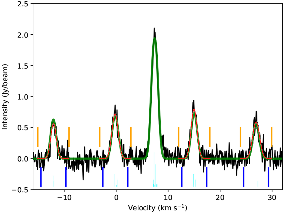
Example of an observed NH₃ (1,1) spectrum with a fitted velocity dispersion of 0.495 km s⁻¹. The black line presents the observed spectrum. The green line presents the result of the 18 hyperfine components fitting. The thick orange vertical lines show the ranges of the sub-spectra used to fit the inner and outer satellite lines with single Gaussian functions. The thick blue vertical lines below the zero level show the ranges used to calculate the integrated hyperfine intensity anomalies of the inner and outer satellite lines. The red lines indicate the single Gaussian fitting results. The cyan vertical lines below the zero level present the 18 hyperfine individual components listed Table A.1. The lengths and separations of these cyan lines denote their expected intensities and velocity separations.