| Issue |
A&A
Volume 691, November 2024
|
|
|---|---|---|
| Article Number | A111 | |
| Number of page(s) | 8 | |
| Section | Interstellar and circumstellar matter | |
| DOI | https://doi.org/10.1051/0004-6361/202450919 | |
| Published online | 31 October 2024 | |
NH3 (1,1) hyperfine intensity anomalies in infall sources
1
Xinjiang Astronomical Observatory,
CAS 150, Science 1-Street Urumqi,
Xinjiang
830011,
China
2
Max-Planck-Institut für Radioastronomie,
Auf dem Hügel 69,
53121
Bonn,
Germany
★ Corresponding author; This email address is being protected from spambots. You need JavaScript enabled to view it.
Received:
30
May
2024
Accepted:
11
September
2024
Abstract
Identifying infall motions is crucial for our understanding of accretion processes in regions of star formation. The NH3 (1,1) hyperfine intensity anomaly (HIA) has been proposed to be a readily usable tracer for such infall motions in star-forming regions harboring young stellar objects at very early evolutionary stages. In this paper, we seek to study the HIA toward 15 infall candidate regions in order to assess its reliability as an infall tracer. Using deep observations of the NH3 (1, 1) transition with the Effelsberg 100 m telescope, we identified HIAs toward all 15 targets. Of the 15 sources, 14 exhibit anomalous intensities in either the inner or outer satellite lines. All the derived HIAs conform to the framework of the existing two models, namely hyperfine selective trapping (HST) and systematic contraction or expansion motion (CE) models. In our sample of infall candidates, the majority of the HIAs remain consistent with the HST model. Only in three targets are the HIAs consistent with infall motions under the CE model. Thus, the HIA could indeed be used as an infall tracer, but does not appear to be highly sensitive to infall motions in our single-dish data. Nevertheless, the emission could be blended with emission from outflow activities. HIAs consistent with the HST model show stronger anomalies with increasing kinetic temperatures (TK), which is expected based on the HST model. On the other hand, HIAs consistent with infall motions show little dependence on Tk . Therefore, HIAs may preferably trace the infall of cold gas.
Key words: stars: formation / ISM: clouds / ISM: kinematics and dynamics / ISM: molecules
© The Authors 2024
 Open Access article, published by EDP Sciences, under the terms of the Creative Commons Attribution License (https://creativecommons.org/licenses/by/4.0), which permits unrestricted use, distribution, and reproduction in any medium, provided the original work is properly cited.
This article is published in open access under the Subscribe to Open model. This email address is being protected from spambots. You need JavaScript enabled to view it. to support open access publication.
1 Introduction
Accretion is a fundamental phenomenon in the process of star formation (e.g., Shu 1977; Mac Low & Klessen 2004). However, observational evidence of gas infall motions has remained inconclusive (e.g., Evans 1999; Evans et al. 2015). Blue-skewed line profiles of optically thick lines serve as readily accessible tracers of infall motions, and rely on excitation gradients within the clump (e.g., Leung & Brown 1977; Zhou et al. 1993). Given higher excitation temperatures toward the center, the inward motion of the clump will manifest itself in more pronounced blueshifted emission (Zhou et al. 1993; Evans 1999). Nevertheless, there are also alternative explanations, such as chemical variations and rotation (e.g., Evans 2003). At the same time, blue-skewed line profiles observed by single-dish telescopes may be blended with red-skewed profiles caused by outflow activities. Additionally, the requirement of elevated excitation toward the center means that the blue-skewed emission becomes less pronounced, making it a less powerful infall tracer for objects in very early evolutionary stages with lower radial changes of the excitation temperature.
Searching for redshifted absorption features against radio or millimeter continuum emission appears to be a promising approach (e.g., Di Francesco et al. 2001; Wyrowski et al. 2012; Yang et al. 2022). The inverse P-Cygni profile, which is characterized by redshifted absorption and blueshifted emission, is a relatively robust infall indicator, because these profiles largely confirm that the gas moving inwards (redshifted) is in front of the central source. Observations with high-angular-resolution interferometers are usually required to confirm infall toward the central continuum source (e.g., Beltrán et al. 2022). Because of the optically thick nature of the dust emission at frequencies of ≳1 THz, absorption lines are more readily observed in this frequency range. Wyrowski et al. (2016) employed the Stratospheric Observatory for Infrared Astronomy (SOFIA) at ~1.8 THz and detected redshifted absorption features toward high-mass star-forming regions. Additionally, the authors noted that these redshifted absorption features are often not significantly contaminated by redshifted outflowing gas. However, acquiring new data for these high-frequency absorption lines – which are beyond the capabilities of ground-based telescopes – is not possible after the end of the SOFIA mission.
In all the aforementioned methods, optically thin lines are usually required to trace the systemic velocities, delineating the boundary between the blue- and redshifted features and ruling out the possibility of two separate velocity components. Efforts are ongoing to improve our capacity for detecting infall motions, with the aim being to achieve a comprehensive understanding of these motions in star-forming regions across a wider range of evolutionary stages and spatial scales. In the present study, we test the viability of using ammonia hyperfine intensity anomalies (HIAs) as a promising infall tracer.
The microwave frequency inversion transitions of ammonia (NH3) are frequently used tracers in studies of star-forming regions, molecular clouds, and nearby galaxies (e.g., Zhang et al. 1998; Henkel et al. 2005; Lu et al. 2014; Wu et al. 2018). The ground-state para NH3 (J, K) = (1,1) transition comprises five distinct groups of hyperfine structure (hfs) components originating from electric quadrupole splitting. These components include the main line (∆F1 = 0, where F1 is the quantum number of the electric quadrupole coupling hyperfine components and four satellite lines (∆F1 = ±l), with two on each side of the main line (Ho & Townes 1983). The presence of weaker magnetic spin-spin interactions results in a total of 18 hyperfine components distributed over the profiles of the five lines (e.g., Rydbeck et al. 1977). Under conditions of local thermodynamic equilibrium (LTE) and optically thin emission, the two inner satellite line groups (ISLs) and the outer satellite line groups (OSLs) are anticipated to have the same intensities (26% for each ISL and 22% for each OSL of the main line intensity; e.g., Ho & Townes 1983). However, the expectation of equal intensities for the ISLs and OSLs is not always valid (e.g., Matsakis et al. 1977; Camarata et al. 2015). Non-LTE populations between the substates of the NH3 (1, 1) level, which give rise to HIAs, can be attained by (1) hyperfine selective trapping (HST) from NH3 (2, 1) to (1, 1) levels (e.g., Matsakis et al. 1977; Stutzki & Winnewisser 1985) and/or (2) systematic contraction or expansion motions (CE) (e.g., Park 2001). It is possible to distinguish between these two models, because they predict different relative intensities of the satellite lines (see Sect. 4.1). Under the CE model, redshifted and blueshifted photons (due to systematic motions) emitted from one hyperfine transition can be absorbed by another one, resulting in substantial changes in the level populations of the NH3 (1 , 1) sublevels. Contraction and expansion can enhance the emission of the two satellite lines on the blue and red side, respectively, while suppressing those on the other side (e.g., Park 2001). Thus, the HIA is expected to serve as a tracer of systematic motions without relying on the detailed analysis of line shapes (Park 2001).
In summary, the HIA, as an infall tracer, exhibits two enhanced blueshifted satellite lines, and resembles a discrete version of the blue-skewed profile, albeit with different underlying physics. The presence of five well-separated components in the NH3 (1, 1) transition enables the straightforward identification of enhanced emission. Furthermore, the HIA is based on the cross-absorption between the hyperfine transitions. In principle, higher excitation toward the center is not required. For example, in the simulations conducted by Park (2001), obvious HIAs were reproduced in an infalling core with a constant temperature of 15 K. This makes the HIA a promising infall tracer of both star-forming regions and large-scale accretion at very early evolutionary stages. In contrast, blue-skewed profiles can reliably trace the infall motion around a hot core (Evans 2003).
Nonetheless, the relative contribution of systematic motions to HIAs remains a matter of debate (e.g., Longmore et al. 2007; Wienen et al. 2018; Zhou et al. 2020). In these studies, HIAs tend to be consistent with the HST model. However, the infall motions of the targets in these studies were not confirmed. Hence, in the present paper, we seek to investigate HIAs toward 15 infall candidates – identified by their blue-skewed or redshifted absorption profiles – to test whether the HIA can be used as an infall tracer.
Targets and observational parameters.
2 Targets and observations
2.1 Targets
We selected 15 infall candidates from the literature (see Table 1). Blue-skewed profiles were extensively observed in B335, for example by the Institute de Radioastronomie Millimétrique (IRAM) 30m telescope in H2CO (212−111), CS (2−1), (3−2), and (5−4), and by the Caltech Submillimeter Observatory (CSO) 10.4 m telescope in HCO+ (3−2) with resolutions ranging from 11″ to 28″ (e.g., Zhou et al. 1993). Inverse P-Cygni profiles were also seen in Atacama Large Millimeter/submillimeter Array (ALMA) HCN (4−3) and HCO+ (4−3) spectra with a resolution of about 0″.5 (Evans et al. 2015). However, recent high-resolution ALMA observations of optically thin tracers revealed the presence of two velocity components that could contribute to the double-peaked line profiles (e.g., Cabedo et al. 2021).
Infall indicators were also widely identified in G031.41+0.31. For example, a redshifted absorption profile was identified in the SOFIA NH3 32+−22− line with a resolution of about 16″ (Wyrowski et al. 2012). Meanwhile, blue-skewed profiles were detected in the HCO+ (4−3), HNC (4−3), and HCN (4−3) lines observed by the Atacama Pathfinder Experiment 12 meter submillimeter telescope (APEX) and in the CS (2−1) line observed with the IRAM 30 m telescope, with resolutions ranging from 17″ to 27″ (Wyrowski et al. 2016). Inverse P-Cygni profiles were also detected in dense cores with ALMA spectra of CH3CN (12−11) and H2CO (30,3−20,2), (32,2−22,1), and (32,ı−22,0) with resolutions of about 0″.1 (e.g., Beltrán et al. 2022).
The inverse P-Cygni profile in IRAS 18360-0537 was observed near the dust peak MM1 using the Submillimeter Array (SMA) in the CN (2−1) line with a resolution of about 1″.4 (Qiu et al. 2012). Blue-skewed profiles were also identified with the CSO in HCN (3−2) and the Arizona Radio Observatory (ARO) 12m telescope in HCO+ (1−0) with resolutions of 27″ and 70″, respectively (Yoo et al. 2018).
G023.21−0.3, G034.26+0.2, and G035.20−0.7 were selected from Wyrowski et al. (2016). In these three targets, redshifted absorption features were observed using the SOFIA in the NH3 32+−22− line at a resolution of about 16″. Furthermore, blue-skewed profiles were identified in all three targets through HCO+ (4−3) observed with APEX with a resolution about 17″ (Wyrowski et al. 2016). As also reported in Wyrowski et al. (2016), in the case of G023.21−0.3, APEX HNC (4−3) observations with a resolution of 16″ revealed blue-skewed profiles. Similarly, in the case of G034.26+0.2, APEX HCN (4−3) observations with a resolution of 17″ showed blue-skewed profiles. Regarding G035.20-0.7, IRAM 30m HCO+ (1−0) observations with a resolution of 28 revealed the presence of blue-skewed profiles.
BGPS 3604, BGPS 4029, and BGPS 5021 were selected from Calahan et al. (2018). Blue-skewed profiles were observed in the three targets using ARO 12 m single-pointing HCO+ (1−0) observations with a resolution of about 68 (Calahan et al. 2018). Yang et al. (2021) mapped G029.60−0.63, G053.13+0.09, G081.72+0.57, G082.21−1.53, G121.31+0.64, and G193.01+0.14 with the IRAM 30m telescope at a resolution of about 28 . In all of these six targets, blue-skewed profiles were detected in the HCO+ (1−0) line toward the positions showing the strongest H13CO+ (1−0) emission (Yang et al. 2021).
2.2 NH3 observations
Deep NH3 observations (PI: Gang Wu, project ID: 15-21) were conducted in February 2022 with the Effelsberg 100 m telescope1. The K-band double-beam and dual-polarization receiver was employed as the frontend. The fast Fourier transform spectrometer (FFTS) at that facility was used as backend, which offered two frequency windows with bandwidths of 300 MHz and 65536 channels each. This results in a channel width of about 4.6 kHz, corresponding to a velocity spacing of about 0.06 km s−1 at 23.7 GHz. The three metastable NH3 (J, K) = (1, 1), (2, 2), and (3, 3) lines, along with the  water maser transition, were observed simultaneously. Spectral calibration was applied following the method described by Winkel et al. (2012). NGC 7027 was used to obtain the initial pointing and the focus corrections and to calibrate the spectral line flux, assuming a continuum flux density of 5.7 Jy at 23.7 GHz (Ott et al. 1994). At the NH3 frequencies, the full width at half maximum (FWHM) beam size is about 37″ and the main beam efficiency is 60%. The conversion factor from the flux density scale to the main beam brightness temperature is 1.73 KJy−1. The focus was checked every few hours and the pointing was calibrated every hour by observing nearby compact continuum sources. A position-switching mode was used in the observations with the off position at an offset of 900 from each target in azimuth As achieving good signal-to-noise ratios for the NH3 (1 , 1) satellite lines is crucial in order to establish a robust HIA (e.g., Zhou et al. 2020), the total on + off integration time on each target exceeds 70 minutes and 1σ noise levels are about 50 mK on a Tmb scale for a channel width of 0.06 km s−1 (see Table 1). We note that NH3 (1, 1) hyperfine features were all measured simultaneously, thus ensuring an accurate relative calibration.
The GILDAS/CLASS software developed by IRAM was mainly used for the data reduction. All of the spectra have flat and gently varying baselines, meaning that only linear baselines had to be subtracted.
3 Results
Thanks to the long integration times on the targets (see Table 1), all of the NH3 satellite lines are clearly detected (see Fig. 1). This is important for unambiguously determining the HIAs and distinguishing between the HIA models (see Sect. 1 and below). As discussed in Zhou et al. (2020), the HIA calculated with peak intensities from Gaussian fittings does not accurately reflect the true anomaly. That is because the red- and blueshifted ISLs (OSLs), which are the combination of Gaussian spectra of three (or two) hyperfine components with different offsets (see the blue vertical lines in Fig. 1), should exhibit different line widths and peak intensities even under LTE and optically thin conditions (see Appendix A in Zhou et al. 2020). Zhou et al. (2020) determine the HIA as the ratio of the red- to blueshifted integrated intensities, and we largely follow their recipe. Specifically, we first used the combined 18 Gaussian hyperfine components to fit the observed NH3 (1, 1) spectra. Then, based on the fitted central velocity and velocity dispersion, we defined the integrated velocity ranges (see the red vertical lines in Fig. 1). Finally, we calculated the HIAs of the ISL (HIAIS) and OSL (HIAOS) as the ratio of their redshifted to blueshifted integrated intensities from the observed spectra:
 (1)
(1)
 (2)
(2)
where Frisl/Frosl and Fbisl/Fbosl are the integrated intensities of the red- and blueshifted sides of the ISLs and OSLs, respectively. The standard deviation σHIA of HIAs is assigned by
 (3)
(3)
where HIA is the value of either HIAIS or HIAOS, NC is the channel number within the integrated range, σBL is the noise level of the baseline, and FR and FB are the integrated intensities of the redshifted and blueshifted sides of the ISLs or OSLs.
The distribution of observed HIAIS and HIAOS values of the 15 targets is also shown in Fig. 2. Unity indicates no anomaly. In 14 out of 15 targets, either HIAIS or HIAOS deviates from unity by more than σHIA, and in 10 of these targets, both HIAIS and HIAOS values exceed σHIA. Thus the presence of HIAs is prevalent in our sample. The two dashed lines in Fig. 2 divide the HIAIS and HIAOS data into four quadrants: quadrants I (HIAIS > 1 and HIAOS > 1), II (HIAIS < 1 and HIAOS > 1), III (HIAIS < 1 and HIAos < 1), and IV (HIAIS > 1 and HIAOS < 1). These quadrants can be used to distinguish different HIA models (see Sect. 4.1). From Fig. 2 we can see that 1 (6.7%), 11 (73.3%), 3 (20%), and 0 data points are located in quadrants I, II, III, and IV (0, 7 (46.7%), 3 (20%), and 0, respectively, considering 1σ uncertainties). Based on our deep observations these fractions in the four quadrants are generally consistent with previous statistical results (e.g., Wienen et al. 2018; Zhou et al. 2020).
In the cases of IRAS 18360−0537, G031.41+0.31, G034.26+0.2, and G081.72+0.57, there is significant blending between their main lines and ISLs. This may impact the determination of the HIAIS, if the main line has asymmetric profiles, which contribute differently to the two ISLs. Below, we qualitatively discuss the potential corrections for the line blending. Taking IRAS 18360-0537 as an example, as seen in the first panel of Fig. 1, the asymmetric main line contributes more flux to the blueshifted ISL than to the redshifted ISL. Thus, the real HIAIS might be larger than the calculated one, as indicated by the arrow in Fig. 2. However, we should note that the length of the arrow is not quantitatively proportional to the corrections, as it is difficult to precisely determine the contribution of the blending main line. For all of these four targets, we label the potential corrections with arrows in Fig. 2. We can see that, for G031.41+0.31 and G081.72+0.57, their actual HIAIS should be smaller than the calculated one. Thus, these corrections do not alter their quadrants. For the other two targets, especially IRAS 18360-0537, whose HIAIS is closer to unity, the line-blending effect might change their quadrant from II to I.
We should note that changes in the relative intensities of the ISL or OSL may occur due to large opacities. Theoretically, each ISL (OSL) contains three (two) identical hyperfine components, as indicated by the blue vertical lines in Fig. 1. However, as mentioned above, while the intensities of the hyperfine components are the same, the frequency separations between them vary, as represented by the spacing of the blue vertical lines in Fig. 1. In high-opacity scenarios, satellites with smaller separations between hyperfine components may achieve saturation more rapidly than those with larger separations. Therefore, we also derived the opacities of the ISL and OSL for all the spectra by summing up the opacities of their respective hyperfine components (see Table 1). The ISLs and OSLs in our spectra tend to be optically thin, with the exceptions of those of G035.2–0.7 and G023.21–0.3, which show moderate opacities of about 0.6. Therefore, the opacities should not result in a significant intensity difference between the two ISLs/OSLs.
As discussed in Zhou et al. (2020), the deviations of the HIA defined by peak intensities from the true HIA become more pronounced for spectra with narrow line widths. We can see from Fig. 3 – taking B335 as an example – that the peak intensity of the blueshifted OSL is larger than that of the redshifted one, simply because the separation of the two hyperfine components within the blueshifted OSL is smaller than that of the redshifted OSL (see the blue vertical lines in Fig. 2). From Fig. 2 we see that HIAOS of B335 is actually larger than unity (the integrated intensity of the blueshifted OSL is smaller than that of the red- shifted one). We refer to Appendix A in Zhou et al. (2020) for detailed comparisons between the HIAs defined by peak and integrated intensity ratios. In addition, at the resolution of 37″, our observations may encompass a number of cloud or velocity components, which are more evident in the case of G31.41+0.31 and IRAS 18360–0537, which show slight deviations from Gaussian profiles (see Fig. 1). While the limited angular resolution of our data is ideal for the determination of the gross HIA, it does not permit an evaluation of the spatial fine structure, which might reveal more than one velocity component within the targeted area.
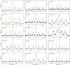 |
Fig. 1 Observed NH3 (J, K) = (1, 1) spectra. In each panel, the green curve represents the fit to 18 hyperfine lines and the blue vertical lines under the spectrum indicate the positions of the 18 hyperfine lines and their relative strengths in the optically thin case under conditions of LTE. The red lines denote the integrated ranges used to calculate the HIA. The source name is labeled in the top-left corner of each panel. |
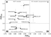 |
Fig. 2 Distribution of the hyperfine intensity anomalies of the inner (HIAIS) and outer (HIAOS) satellite lines. Arrows indicate potential corrections for the blending of the primary and inner satellite lines. The source name is marked in close proximity to each data point. Gray dashed vertical and horizontal lines divide the panel into four subregions: I for HIAIS > 1 and HIAOS > 1, II for HIAIS < 1 and HIAOS > 1, III for HIAIS < 1 and HIAOS < 1, and IV for HIAIS > 1 and HIAOS < 1. The models that cause HIAs to be located in these subregions are also labeled. |
4 Discussion
4.1 HIA sensitivity to infall motions
The HST and CE models predict distinct HIAs (e.g., Zhou et al. 2020). According to the HST model, the intensity of the blueshifted ISL is expected to be greater than that of the redshifted one, while the redshifted OSL should exhibit greater intensity than the blueshifted one. Thus, HIAIS < 1 and HIAOS > 1 (quadrant II; e.g., Stutzki & Winnewisser 1985; Camarata et al. 2015). In the context of the CE model (e.g., Park 2001), for infall motions, both the blueshifted ISL and OSL are anticipated to be stronger than the two redshifted lines, that is HIAIS < 1 and HIAOS < 1 (quadrant III). Conversely, for expansion motions, the redshifted ISL and OSL are expected to exhibit greater intensity simultaneously, that is HIAIS > 1 and HIAOS > 1 (quadrant I). As discussed in Zhou et al. (2020), we can employ the HIA quadrant plot of HIAIS and HIAOS to identify the HIA models (see the different models labeled in the four subregions of Fig. 2).
From Fig. 2, it is noteworthy that all the derived HIAs remain within the framework of the two models, with no data points in the forbidden quadrant IV. However, it is somewhat unexpected that a majority of the HIAs are located in the second quadrant, aligning with the HST model. This indicates that, in our observations, the HST model is the predominant model, even in sources likely harboring infall motions. However, alternative explanations exist. Similar to the case of blue-skewed profiles, the observed features might be blended with emission from outflows (e.g., Evans 2003; Wyrowski et al. 2016). This phenomenon is also applicable to HIAs, as ammonia emission is also commonly seen in outflows (e.g., Zhang et al. 2007). This could only be further clarified through interferometer observations, which are capable of resolving distinct structures.
There are three data points located in quadrant III, indicating the potential existence of infall motions. For these three sources, infall motions should be widespread within the beam size of about 37″. Increased kinetic temperatures would enhance the HST HIAs (e.g., Stutzki & Winnewisser 1985) and could also lead to more ammonia molecules being excited to the NH3 (2,1) level. Consequently, the likelihood increases that the sources will be better explained by the HST model. Therefore, HIAs may be preferable infall tracers in star-forming regions at early evolutionary stages. However, we do not find a preferred evolutionary stage among these three targets in quadrant III. BGPS 4029, G029.60–0.63, and G031.41+0.31 were reported to be associated with an infrared-dark cloud (IRDC; Peretto & Fuller 2009), Class 0/I YSOs (Yang et al. 2020), and a massive protocluster, respectively (Beltrán et al. 2022). Nevertheless, HIAs may indeed be used as an infall tracer for early evolutionary stages, such as IRDCs.
As mentioned above, in the HST model, the ISL and OSL exhibit reversed anomalous intensities (HIAIS < 1 and HIAOS > 1). In the CE model, infall motions enhance both the blueshifted ISL and OSL, while expansion motions enhance both the red- shifted ISL and OSL (HIAIS < 1 and HIAOS < 1 for infall motions, HIAIS > 1 and HIAOS > 1 for expansion motions). As a result, using the ratio between the sum of the intensities of the two redshifted satellite lines and the sum of the intensities of the two blueshifted satellite lines, the influence of the HST model (the ISL and OSL exhibit reversed anomalies) would be mitigated and that of the CE model would be enhanced. Therefore, we also study the ratio HIAISOS:
 (4)
(4)
We should note that it is unclear whether or not the anomalous fluxes of the blueshifted ISL and the redshifted OSL are precisely equal in the HST model (e.g., Stutzki & Winnewisser 1985).
Figure 3 shows the distribution of HIAISOS. Of the 15 sources, 8 (6, considering uncertainties) are consistent with infall motions. Indeed, more sources exhibit consistency with infall motions than those in quadrant III of Fig. 2. This outcome demonstrates that HIAISOS could be a better infall tracer than HIAIS or HIAOS. However, HIAISOS may also not be an ideal indicator of infall for our data. Taking uncertainties into account, there are only six reliable data points of HIAISOS that are consistent with infall motions in this sample of infall candidates. Naturally, the three sources already previously suggested to represent infall (quadrant III sources in Fig. 2) are part of this subsample.
In summary, in our single-dish observations, most of the detected HIAs are consistent with the HST model. HIAs could be used as an infall tracer but do not seem to be highly sensitive to infall motions. High-resolution observations would be essential for a more precise assessment of the contaminating impact of outflows.
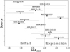 |
Fig. 3 Distribution of the combined hyperfine intensity anomalies. The source name is labeled above each data point. |
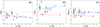 |
Fig. 4 Correlations of HIAIS and TK (panel a), HIAOS and TK (panel b), and HIAISOS and TK (panel c). The HIAs consistent with the HST model and CE model (infall motions) are emphasized in blue and red colors, respectively. Blue and red lines indicate their linear regression results. Linear fit parameters for the blue and red lines are given in Table 2. |
4.2 HIAs versus kinetic temperature
As mentioned above, higher temperatures can potentially lead to the dominance of the HST model. In this section, we explore the correlation between HIAs and the kinetic temperature (TK). NH3 inversion transitions are an invaluable spectroscopic probe of TK (Ho & Townes 1983). We derive the rotational temperature TR from the observed para-NH3 (1,1) and (2,2) spectral lines (see Fig. A.1) using the PySpecKit package (Ginsburg & Mirocha 2011), which is a forward-modeling tool for spectral lines. Then, TK is calculated following Tafalla et al. (2004) as
![Mathematical equation: ${T_{\rm{K}}} = {{{T_{\rm{R}}}} \over {1 - {{{T_{\rm{R}}}} \over {42}}\ln \left[ {1 + 1.1\exp \left( { - 16/{T_{\rm{R}}}} \right)} \right]}}.$](/articles/aa/full_html/2024/11/aa50919-24/aa50919-24-eq6.png) (5)
(5)
Tafalla et al. (2004) conducted various Monte Carlo simulations involving data for the NH3 (1,1), (2,1), and (2,2) transitions in order to derive an analytical expression with which to estimate TK from TR. TK can be very well approximated by this equation in the range TK = 5–20 K. It is important to note that the applicability of this approximation diminishes at higher temperatures. Figure 4 shows the correlations between HIAs (HIAIS, HIAOS, and HIAISOS) and TK. The HIAs consistent with the HST model and the CE model (infall motions) are emphasized in blue and red, respectively. Meanwhile, their linear regression results are also shown in each panel (blue and red lines) and in Table 2.
We first see from the blue data points in panels a and b of Fig. 4 that HIAIS and HIAOS all tend to show rising deviations from unity (indicating higher anomalies) with increasing TK, which is expected based on the HST model. We should note that the correlations are weak, with correlation coefficients of −0.29 and −0.12 for HIAIS and HIAOS, respectively (see Table 2). This may be attributed to the considerable dispersion among these data points, which is especially high for HIAOS as determined by the relatively weak OSLs. While the HST model predominantly influences the blue data points, the CE model may also play a minor role, introducing additional uncertainties. For example, the two HIA models produce contrasting predictions concerning the enhancement of the OSLs.
HIAs consistent with infall motions are not expected to exhibit a dependence on TK. In our observations, both HIAIS and HIAOS, indicated in red, appear to show a constant value that is independent of TK. It is essential to note that the sample size is limited; the sample consists of only three data points. Therefore, subsequent comparisons of potential trends in HIAs against TK are tentative. The slope of HIAIS appears more negative compared to that of HIAOS. In general, HIAs induced by infall motions (red data points) demonstrate relatively low sensitivity to TK compared to HIAs consistent with the HST model (blue data points in Fig. 4). This outcome implies that HIAs might serve as more effective infall tracers for relatively cold gas, which may help us to understand the large-scale accretion and infall motions in early evolutionary star-forming cores.
Finally, in panel c of Fig. 4, we can see from the blue data points that, in general, the HIAISOS of the targets associated with the HST model are very close to unity. Therefore, HIAISOS could largely weaken the impact of the HST model, as explained above (see Fig. 3). This indicates that the anomalous fluxes of the ISL and OSL are comparable within the HST model. The red data points (i.e., those associated with infall motions) are not affected by such a consideration, because their blueshifted ISLs and OSLs are enhanced simultaneously.
Parameters for the linear regressions.
5 Summary
We conducted deep observations of the ammonia hyperfine intensity anomalies (HIAs) with the Effelsberg 100 m telescope in 15 infall source candidates. By adopting a rational definition of the HIA proposed by Zhou et al. (2020), we seek to test whether or not HIAs can be used to trace infall motions, in particular of the cold molecular gas. Due to long integration times on the targets, all the NH3 satellite lines are clearly detected and all the HIAs of the inner (HIAIS) and outer (HIAOS) satellite lines are derived. In 14 out of 15 targets, either HIAIS or HIAOS values deviate from unity (indicating an anomaly) by more than their 1σ uncertainties. In 10 targets, both HIAIS and HIAOS values exceed their 1σ uncertainties. Thus, the presence of HIAs is prevalent in our sample. Meanwhile, all the derived HIAs remain within the framework of the existing two models, namely the hyperfine selective trapping (HST) model and the systematic contraction or expansion motion (CE) model. We find that the majority of the HIAs in the sources likely harboring infall motions are still consistent with the HST model. In three sources, HIAs are consistent with infall motions under the CE model, while a procedure mitigating the effects of the HST model even uncovers six such sources. Therefore, HIAs could be used as an infall tracer but do not seem to be highly sensitive to infall motions in our single-dish observations. Nevertheless, akin to the case of blue-skewed profiles, HIAs might be blended with emission from outflow activities, as ammonia emission is also commonly seen in outflows.
HIAs induced by the HST model are expected to be enhanced with increasing kinetic temperatures (TK). HIAIS and HIAOS in our observations may show higher anomalies with increasing TK, but the correlations are weak. On the contrary, HIAs induced by infall motions seem to show relatively constant values over a range of TK, suggesting that HIAs might serve as more effective infall tracers for relatively cold gas. High-resolution observations of HIAs are crucial to further constrain the origin of HIAs and to assess the contributions from infall and outflow motions.
Acknowledgements
We thank the anonymous referee for useful suggestions improving the paper. Based on observations with the 100-m telescope of the MPIfR (Max-Planck-Institut für Radioastronomie) at Effelsberg. This work was funded by the National Key R&D Program of China (No. 2022YFA1603103), the CAS “Light of West China” Program (No. 2021-XBQNXZ-028), the National Natural Science foundation of China (Nos.12103082, 11603063, and 12173075), and the Natural Science Foundation of Xinjiang Uygur Autonomous Region (No. 2022D01A362). GW acknowledges the support from Youth Innovation Promotion Association CAS.
Appendix A Observed NH3 (J, K) = (1,1) and (2,2) spectra
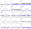 |
Fig. A.1 NH3 (J, K) = (1,1) and (2, 2) spectra. The observed NH3 (J, K) = (1, 1) and (2, 2) spectra are shown in black and blue in each panel. NH3 (J, K) = (2, 2) spectra are shifted to −0.2 K on the Y-axis. The source name is given in the top-left corner of each panel. |
References
- Beltrán, M. T., Rivilla, V. M., Cesaroni, R., et al. 2022, A&A, 659, A81 [NASA ADS] [CrossRef] [EDP Sciences] [Google Scholar]
- Camarata, M. A., Jackson, J. M., & Chambers, E. 2015, ApJ, 806, 74 [NASA ADS] [CrossRef] [Google Scholar]
- Calahan, J. K., Shirley, Y. L., Svoboda, B. E., et al. 2018, ApJ, 862, 63 [NASA ADS] [CrossRef] [Google Scholar]
- Cabedo, V., Maury, A., Girart, J. M., et al. 2021, A&A, 653, A166 [NASA ADS] [CrossRef] [EDP Sciences] [Google Scholar]
- Di Francesco, J., Myers, P. C., Wilner, D. J., et al. 2001, ApJ, 562, 770 [NASA ADS] [CrossRef] [Google Scholar]
- Evans, N. J. 1999, ARA&A, 37, 311 [NASA ADS] [CrossRef] [Google Scholar]
- Evans, N. 2003, SFChem 2002: Chemistry as a Diagnostic of Star Formation, 157 [Google Scholar]
- Evans, N. J., Di Francesco, J., Lee, J.-E., et al. 2015, ApJ, 814, 22 [CrossRef] [Google Scholar]
- Ginsburg, A., & Mirocha, J. 2011, Astrophysics Source Code Library [record ascl:1109.001] [Google Scholar]
- Henkel, C., Jethava, N., Kraus, A., et al. 2005, A&A, 440, 893 [NASA ADS] [CrossRef] [EDP Sciences] [Google Scholar]
- Ho, P. T. P., & Townes, C. H. 1983, ARA&A, 21, 239 [NASA ADS] [CrossRef] [Google Scholar]
- Immer, K., Li, J., Quiroga-Nuñez, L. H., et al. 2019, A&A, 632, A123 [NASA ADS] [CrossRef] [EDP Sciences] [Google Scholar]
- König, C., Urquhart, J. S., Csengeri, T., et al. 2017, A&A, 599, A139 [Google Scholar]
- Leung, C. M., & Brown, R. L. 1977, ApJ, 214, L73 [NASA ADS] [CrossRef] [Google Scholar]
- Longmore, S. N., Burton, M. G., Barnes, P. J., et al. 2007, MNRAS, 379, 535 [NASA ADS] [CrossRef] [Google Scholar]
- Lu, X., Zhang, Q., Liu, H. B., Wang, J., & Gu, Q. 2014, ApJ, 790, 84 [NASA ADS] [CrossRef] [Google Scholar]
- Mac Low, M.-M., & Klessen, R. S. 2004, Rev. Mod. Phys., 76, 125 [Google Scholar]
- Matsakis, D. N., Brandshaft, D., Chui, M. F., et al. 1977, ApJ, 214, L67 [NASA ADS] [CrossRef] [Google Scholar]
- Ott, M., Witzel, A., Quirrenbach, A., et al. 1994, A&A, 284, 331 [NASA ADS] [Google Scholar]
- Park, Y.-S. 2001, A&A, 376, 348 [NASA ADS] [CrossRef] [EDP Sciences] [Google Scholar]
- Peretto, N., & Fuller, G. A. 2009, A&A, 505, 405 [NASA ADS] [CrossRef] [EDP Sciences] [Google Scholar]
- Qiu, K., Zhang, Q., Beuther, H., et al. 2012, ApJ, 756, 170 [NASA ADS] [CrossRef] [Google Scholar]
- Rydbeck, O. E. H., Sume, A., Hjalmarson, A., et al. 1977, ApJ, 215, L35 [NASA ADS] [CrossRef] [Google Scholar]
- Shu, F. H. 1977, ApJ, 214 [Google Scholar]
- Stutzki, J., & Winnewisser, G. 1985, A&A, 144, 13 [NASA ADS] [Google Scholar]
- Svoboda, B. E., Shirley, Y. L., Battersby, C., et al. 2016, ApJ, 822, 59 [Google Scholar]
- Tafalla, M., Myers, P. C., Caselli, P., et al. 2004, A&A, 416, 191 [NASA ADS] [CrossRef] [EDP Sciences] [Google Scholar]
- Watson, D. M. 2020, RNAAS, 4, 88 [NASA ADS] [Google Scholar]
- Wienen, M., Wyrowski, F., Menten, K. M., et al. 2018, A&A, 609, A125 [NASA ADS] [CrossRef] [EDP Sciences] [Google Scholar]
- Winkel, B., Kraus, A., & Bach, U. 2012, A&A, 540, A140 [NASA ADS] [CrossRef] [EDP Sciences] [Google Scholar]
- Wu, G., Qiu, K., Esimbek, J., et al. 2018, A&A, 616, A111 [NASA ADS] [CrossRef] [EDP Sciences] [Google Scholar]
- Wu, G., Henkel, C., Xu, Y., et al. 2023, A&A, 677, A80 [NASA ADS] [CrossRef] [EDP Sciences] [Google Scholar]
- Wyrowski, F., Güsten, R., Menten, K. M., et al. 2012, A&A, 542, L15 [NASA ADS] [CrossRef] [EDP Sciences] [Google Scholar]
- Wyrowski, F., Güsten, R., Menten, K. M., et al. 2016, A&A, 585, A149 [NASA ADS] [CrossRef] [EDP Sciences] [Google Scholar]
- Xu, Y., Bian, S. B., Reid, M. J., et al. 2021, ApJS, 253, 1 [NASA ADS] [CrossRef] [Google Scholar]
- Yang, Y., Jiang, Z.-B., Chen, Z.-W., et al. 2020, Res. Astron. Astrophys., 20, 115 [CrossRef] [Google Scholar]
- Yang, Y., Jiang, Z., Chen, Z., et al. 2021, ApJ, 922, 144 [NASA ADS] [CrossRef] [Google Scholar]
- Yang, W. J., Menten, K. M., Yang, A. Y., et al. 2022, A&A, 658, A192 [NASA ADS] [CrossRef] [EDP Sciences] [Google Scholar]
- Yoo, H., Kim, K.-T., Cho, J., et al. 2018, ApJS, 235, 31 [NASA ADS] [CrossRef] [Google Scholar]
- Zhang, Q., Hunter, T. R., & Sridharan, T. K. 1998, ApJ, 505, L151 [NASA ADS] [CrossRef] [Google Scholar]
- Zhang, Q., Sridharan, T. K., Hunter, T. R., et al. 2007, A&A, 470, 269 [NASA ADS] [CrossRef] [EDP Sciences] [Google Scholar]
- Zhou, S., Evans, N. J., Koempe, C., et al. 1993, ApJ, 404, 232 [NASA ADS] [CrossRef] [Google Scholar]
- Zhou, D., Wu, G., Esimbek, J., et al. 2020, A&A, 640, A114 [NASA ADS] [CrossRef] [EDP Sciences] [Google Scholar]
The 100-m telescope at Effelsberg is operated by the Max-Planck-Institut für Radioastronomie (MPIfR) on behalf of the Max-Planck-Gesellschaft (MPG).
All Tables
All Figures
|
Fig. 1 Observed NH3 (J, K) = (1, 1) spectra. In each panel, the green curve represents the fit to 18 hyperfine lines and the blue vertical lines under the spectrum indicate the positions of the 18 hyperfine lines and their relative strengths in the optically thin case under conditions of LTE. The red lines denote the integrated ranges used to calculate the HIA. The source name is labeled in the top-left corner of each panel. |
| In the text | |
|
Fig. 2 Distribution of the hyperfine intensity anomalies of the inner (HIAIS) and outer (HIAOS) satellite lines. Arrows indicate potential corrections for the blending of the primary and inner satellite lines. The source name is marked in close proximity to each data point. Gray dashed vertical and horizontal lines divide the panel into four subregions: I for HIAIS > 1 and HIAOS > 1, II for HIAIS < 1 and HIAOS > 1, III for HIAIS < 1 and HIAOS < 1, and IV for HIAIS > 1 and HIAOS < 1. The models that cause HIAs to be located in these subregions are also labeled. |
| In the text | |
|
Fig. 3 Distribution of the combined hyperfine intensity anomalies. The source name is labeled above each data point. |
| In the text | |
|
Fig. 4 Correlations of HIAIS and TK (panel a), HIAOS and TK (panel b), and HIAISOS and TK (panel c). The HIAs consistent with the HST model and CE model (infall motions) are emphasized in blue and red colors, respectively. Blue and red lines indicate their linear regression results. Linear fit parameters for the blue and red lines are given in Table 2. |
| In the text | |
|
Fig. A.1 NH3 (J, K) = (1,1) and (2, 2) spectra. The observed NH3 (J, K) = (1, 1) and (2, 2) spectra are shown in black and blue in each panel. NH3 (J, K) = (2, 2) spectra are shifted to −0.2 K on the Y-axis. The source name is given in the top-left corner of each panel. |
| In the text | |
Current usage metrics show cumulative count of Article Views (full-text article views including HTML views, PDF and ePub downloads, according to the available data) and Abstracts Views on Vision4Press platform.
Data correspond to usage on the plateform after 2015. The current usage metrics is available 48-96 hours after online publication and is updated daily on week days.
Initial download of the metrics may take a while.