| Issue |
A&A
Volume 640, August 2020
|
|
|---|---|---|
| Article Number | A84 | |
| Number of page(s) | 15 | |
| Section | Galactic structure, stellar clusters and populations | |
| DOI | https://doi.org/10.1051/0004-6361/201936570 | |
| Published online | 17 August 2020 | |
Tidal tails of open star clusters as probes of early gas expulsion
I. A semi-analytic model
1
I.Physikalisches Institut, Universität zu Köln, Zülpicher Strasse 77, 50937 Köln, Germany
e-mail: This email address is being protected from spambots. You need JavaScript enabled to view it.
2
Helmholtz-Institut für Strahlen- und Kernphysik, University of Bonn, Nussallee 14-16, 53115 Bonn, Germany
e-mail: This email address is being protected from spambots. You need JavaScript enabled to view it.
3
Charles University in Prague, Faculty of Mathematics and Physics, Astronomical Institute, V Holešovičkách 2, 180 00 Praha 8, Czech Republic
Received:
25
August
2019
Accepted:
17
June
2020
Abstract
Context. Star clusters form in the densest parts of infrared dark clouds. The emergence of massive stars expels the residual gas that has not formed stars yet. Gas expulsion lowers the gravitational potential of the embedded cluster, unbinding many of the cluster stars. These stars then move on their own trajectories in the external gravitational field of the Galaxy, forming a tidal tail.
Aims. We investigate, for the first time, the formation and evolution of a tidal tail that forms due to expulsion of primordial gas. We contrast the morphology and kinematics of this tail with that of another tidal tail that forms by gradual dynamical evaporation of the star cluster. We intend to provide predictions that can determine the dynamical origin of possibly observed tidal tails around dynamically evolved (age ≳ 100 Myr) galactic star clusters by the Gaia mission. These observations might estimate the fraction of the initial cluster population that gets released in the gas expulsion event. The severity of the initial gas expulsion is given by the star formation efficiency and the timescale of gas expulsion for the cluster when it was still embedded in its natal gas. A study with a more extended parameter space of the initial conditions is performed in the follow up paper.
Methods. We provide a semi-analytical model for the tail evolution. The model is compared against direct numerical simulations using NBODY6.
Results. Tidal tails released during gas expulsion have different kinematic properties than the tails gradually forming due to evaporation; the latter kind have been extensively studied. The gas expulsion tidal tail shows non-monotonic expansion with time, where longer epochs of expansion are interspersed with shorter epochs of contraction. The tail thickness and velocity dispersions vary strongly, but not exactly periodically, with time. The times of minima of tail thickness and velocity dispersions are given only by the properties of the galactic potential, and not by the properties of the cluster. The estimates provided by the (semi-)analytical model for the extent of the tail, the minima of tail thickness, and velocity dispersions are in a very good agreement with the NBODY6 simulations. This implies that the semi-analytic model can be used to estimate the properties of the gas expulsion tidal tail for a cluster of a given age and orbital parameters without the necessity of performing numerical simulations.
Key words: galaxies: star formation / stars: kinematics and dynamics / open clusters and associations: general
© ESO 2020
1. Introduction
The problem of star cluster formation has been addressed by two classes of simulations, hydrodynamic simulations and N-body simulations, but there are still many unanswered questions, partly due to the complex interplay between the involved physical processes and partly to the required spatial and temporal resolution of such simulations.
Hydrodynamic simulations usually start from a collapsing cloud, which forms stars, and the stars impact the cloud by their feedback, which in turn opposes the cloud self-gravity and tends to disperse it, suppressing further star formation. The final star formation efficiency (SFE) as well as the masses of individual stars are then given by the regulation of accretion by the multitude of feedback processes. Current state-of-the-art simulations are able to model the formation of only small star clusters (stellar mass of ≈200 M⊙; Bate 2014, see also Bate 2012) that self-consistently form stars with a realistic stellar initial mass function (IMF), which suggests that they contain all important ingredients for star formation and feedback. Simulations aiming at more massive clusters have to resort to coarser approximations; for example, they assume the shape of the IMF (e.g. Dale & Bonnell 2011; Dale et al. 2012; Grudić et al. 2018; Haid et al. 2019) or terminate star formation at some point, remove instantly all gas, and continue with a purely stellar simulation (Fujii 2015; Fujii & Portegies Zwart 2015) and/or take into account only some of the important feedback mechanisms completely neglecting the others (e.g. Gavagnin et al. 2017; Wall et al. 2019). Although these simulations provide valuable insights into the impact of the feedback on the gaseous configuration, their predictive power for the cluster forming mechanisms, which leave imprints for example in the SFE and the dynamics of the natal cluster, is limited at best. Particularly, hydrodynamic simulations give very different prediction to the dispersal of molecular clouds and the SFE even for clouds of comparable masses (see e.g. Dale & Bonnell 2011; Dale et al. 2012 with Gavagnin et al. 2017; Haid et al. 2019).
While hydrodynamic simulations focus on the gaseous phenomena and the stellar dynamics of the young cluster is usually only roughly approximated, N-body simulations adopt a complementary approach: they focus on detailed N-body dynamics at the expense of a rough approximation of gas. In N-body simulations the gas distribution and its evolution is typically described by an analytic formula characterised by several parameters (e.g. the SFE, the timescale of gas removal τM). Since the observational or theoretical constraints on some of these parameters are weak, they are taken as free parameters, and their plausible value is estimated by matching the evolved clusters with observed ones, effectively inverting the problem. In this way, N-body simulations can provide us with a clue not only to the initial conditions of the stellar component, but also to the gas component of natal star clusters.
Basic dynamical arguments distinguish between two different modes of gas expulsion, depending on the duration of the gas expulsion timescale τM relative to the half-mass crossing time th (Hills 1980; Mathieu 1983; Arnold 1989; see also Binney & Tremaine 2008, Chapter 3.6). If the gas is expelled rapidly (impulsively, i.e. τM ≲ th), the cluster is generally more impacted than when the gas is expelled slowly (adiabatic, i.e. th ≪ τM), in which case the cluster gradually expands (e.g. Lada et al. 1984; Goodwin 1997; Kroupa et al. 2001; Baumgardt & Kroupa 2007). The timescale of gas expulsion influences, for example, the minimum value of the SFE, which results in a gravitationally bound star cluster. While rapid gas expulsion means that the SFE needs to be at least ≈30% for formation of a gravitational bound star cluster (Lada et al. 1984; Geyer & Burkert 2001; Kroupa et al. 2001 see also the semi-analytic study of Boily & Kroupa 2003a,b), adiabatic gas expulsion enables cluster formation for substantially lower SFEs, typically 5−10% (Lada et al. 1984; Baumgardt & Kroupa 2007). The existence of evolved bound star clusters (e.g. the Pleiades), which likely contained O stars (these stars expel residual gas quickly due to their powerful feedback), sets a lower limit of the SFE in these systems to ≈30% (Lada & Lada 2003).
Interestingly, some results of N-body simulations seem to contradict the claims of very high SFEs for more massive clusters (mass ≳ 104 M⊙) reported in some hydrodynamic simulations. For example, the rapid expansion of star clusters from their initial subparsec radii (Kuhn et al. 2014; Traficante et al. 2015) by a factor of at least 10 (Pfalzner 2009; Portegies Zwart et al. 2010, and references therein) in ≈10 Myr is not likely to be explained by purely stellar dynamics, but it can be caused by rapid gas expulsion with relatively low SFEs of ≈30% (Banerjee & Kroupa 2017). Furthermore, the approximate virial state of some very young clusters (e.g. R 136; Hénault-Brunet et al. 2012) does not necessarily imply high SFEs because massive clusters revirialise rapidly after gas expulsion (Banerjee & Kroupa 2013).
Some models suggest a relatively low SFE and rapid gas expulsion even in such massive objects as the progenitors of globular clusters. Low SFEs can explain the observed relation (De Marchi et al. 2007) between the concentration of globular star clusters and the slope of their mass function (Marks et al. 2008) as well as the unusual mass function of globular cluster Palomar 14 (Zonoozi et al. 2011) without the need to invoke non-canonical stellar IMFs. The formation of globular clusters with low SFEs can also naturally explain how the globular cluster initial mass function of slope ≈−2 transformed to the currently observed mass function of globular clusters avoiding the assumption of exotic globular cluster initial mass functions (Vesperini 1998; Kroupa & Boily 2002; Parmentier & Gilmore 2005; Baumgardt et al. 2008).
Observationally, the SFE is directly determined only for the nearest star-forming regions, which contain only lower mass star clusters (typically several hundred solar masses at most). These groups and clusters have SFEs mostly in the range 10−30% (Lada & Lada 2003; Megeath et al. 2016). The expansion of the majority (at least 75%, but more probably 85–90%) of young star clusters, which was recently measured thanks to Gaia (Kuhn et al. 2019), presents another piece of evidence for gas expulsion. In addition, the observed offset between the mass function of dense molecular cores and the initial stellar mass function (Alves et al. 2007; Nutter & Ward-Thompson 2007) can be reconciled if cores retain ≈30% of their initial mass during their transformation to stars (Goodwin et al. 2008). For more massive clusters (mass ≳ 104 M⊙), the SFE is observationally less constrained with the possibility that it increases as the clusters consume most of the star-forming gas (Longmore et al. 2014).
A star cluster impacted by rapid gas expulsion with a relatively low SFE of ≈1/3 evolves as follows. First, the stars continue moving with their pre-gas expulsion speeds, but now in a lowered gravitational potential, which results in their outward motions, and expansion of all Lagrangian radii. For this SFE, around 2/3 of all stars escape the cluster. The rest of the stars revirialise, and the Lagrangian radii shrink, with the inner Lagrangian radii decreasing prior to the outer Lagrangian radii. The Lagrangian radii after revirialisation are larger than the initial Lagrangian radii, so revirialisation leaves the cluster rarefied relative to its initial state. After revirialisation the cluster evolves as a purely N-body system with evaporation of the lower mass stars and occasional ejections of predominantly more massive stars (Baumgardt & Makino 2003; Fujii & Portegies Zwart 2011; Perets & Šubr 2012; Oh et al. 2015).
In this case, the cluster loses ≈2/3 of its stars due to gas expulsion during the first Myr of its existence, with subsequent evaporation and ejections taking place afterwards for hundreds of Myr, the cluster losing roughly one star per half-mass crossing time. Since galactic star clusters orbit the Galaxy, the escapers are subjected to the Coriolis force and therefore form two tails: one composed of stars released due to gas expulsion (hereafter tail I) and the other composed of stars released due to evaporation (hereafter tail II)1.
The purpose of this work (hereafter Paper I) and the following paper (Dinnbier & Kroupa 2020, hereafter Paper II) is to constrain the possible range of the SFE by studying the morphology, kinematics, and stellar populations of tidal tails released due to gas expulsion. We take the SFE and the gas expulsion timescale τM as free parameters, and study the properties of the tails as a function of the SFE and τM. A comparison of the modelled tails with the observed ones will provide an independent constraint of the possible value of these fundamental parameters in the cluster formation theory. We expect that the Gaia mission will reveal many tails associated with Galactic star clusters or confirm their absence; both results will be valuable at constraining the parameters. In our modelling we aim particularly at the Pleiades, due to their proximity and age; however, our results can be easily generalised to other star clusters. Throughout this work, the cluster is assumed to orbit the Galaxy in its disc midplane and with zero eccentricity.
It turns out that the morphology and kinematics of tail I and tail II are distinct. Unlike the properties of tail II, which are reasonably well understood (Küpper et al. 2008, 2010), the properties of tail I have not been studied before. Thus, the morphology and kinematics of tail I is addressed in this paper. First, we develop a (semi-)analytical model for some of the most important properties of tail I, and then we compare the model with direct N-body simulations. The N-body simulations in this paper represent only one choice of the SFE and τM, but their purpose is to justify the approximations undertaken in deriving the (semi-)analytical model.
In Paper II, we investigate the influence of the SFE and τM on the formation and evolution of the tidal tails. We also study the cluster mass as another independent parameter. Taking into account the observed properties of the Pleiades cluster, we predict the physical extent and number of stars in the tidal tails for different values of the SFE and τM. For this prediction, we take into account the Gaia accuracy as well as the contamination due to field stars. We also make use of the semi-analytic model of Paper I to extend the models to higher mass clusters than the Pleiades.
2. Semi-analytic model of the gas expulsion tidal tail
2.1. Underlying assumptions and starting equations
Unlike tail II, which is gradually formed as stars evaporate from the cluster over hundreds of Myr, tail I is formed quickly as stars escape the cluster immediately after the gas expulsion event. Accordingly, we assume that all tail I stars escape at time t = 0.
Another difference between tails I and II is the magnitude of velocity of the escaping stars, which determines the allowed directions of escape. As found by Küpper et al. (2010), the majority of stars forming tail II reach a velocity only slightly higher than the velocity needed to escape from the vicinity of Lagrange points L1 and L2 (of the system cluster-Galaxy), but the velocity is lower than required for an escape in other directions. The preferential escape of stars near points L1 and L2 results in the typical S-shape of tail II. Therefore, the speeds of escaping stars are of the order of the difference ΔCJ between the maximum and minimum of the Jacobi potential evaluated at the cluster tidal radius (i.e. at |r|=rt) in the orbital plane. It is straightforward to show that
 (1)
(1)
where G and Mcl is the constant of gravity and the cluster mass, and ω, κ, and ν is the orbital, epicyclic, and vertical frequency of the Galaxy, respectively. This equation provides an escape speed of  for a 4.4 × 10³ M⊙ cluster orbiting the Galactic potential of Allen & Santillan (1991) at the Galactocentric distance of 8.5 kpc. In contrast, the escape speeds
  of stars forming tail I are of the order of the initial velocity dispersion σcl in the embedded star cluster, which is
  , where RV is the cluster virial radius before gas expulsion. A 4.4 × 10³ M⊙ Plummer cluster of acl = 0.23 pc and SFE = 1/3 has σcl = 8.5 km s−1, which is significantly larger than its
  2.
2.
The inequality  holds for any cluster with RV ≲ 2 pc and Mcl ≳ 200 M⊙, so it is likely that it is fulfilled for the majority of star clusters in the current Galactic disc. The inequality implies that the faster stars from tail I are not sensitive to the potential difference at the tidal radius, and they escape the cluster in any direction with the same ease. Thus, in the semi-analytic model, we assume that stars escape isotropically. The validity of the approximation near the threshold
  is explored in Sect. 4.7.
To derive the relevant equations, we adopt the coordinate frame to corotate with the cluster so that the cluster mass centre is at rest in this frame, and it lies at the origin of the coordinate axes (Fig. 1). The x- and y-axes point to the Galactic anticentre and in the direction of Galactic rotation, respectively. The z-axis forms a right-handed system with the x- and y-axes. The cluster orbits the galaxy on a circular orbit of radius R0 and velocity v0, so the radius of the guiding centre of the cluster is thus R0.
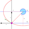 |
Fig. 1. Coordinate frame adopted for deriving the semi-analytic model of tail I. The frame is centred at the star cluster (magenta circle), and the cluster remains at rest in the frame (the frame orbits the Galaxy). The coordinate x- and y-axes, as indicated by thick black arrows, follow the usual convention where the x-axis points towards the galactic anticentre and the y-axis points in the direction of the orbit. The cluster orbits the Galactic centre at radius R0, which corresponds to x = 0 (thick blue line). The green arrow represents the initial trajectory of a star escaping the cluster. After escaping the cluster, the star moves on the red epicycle of semi-minor axis X, semi-major axis Y, and with guiding centre orbiting at Galactic radius Rg, which corresponds to x = X sin α in the adopted coordinates (thin blue line). The meaning of the escape angle α is shown by the blue curved arrow. |
Consider a star escaping from the cluster at velocity with components (vR, vϕ, vz) in the direction (x, y, z). The star then orbits its new guiding centre Rg on an ellipse with semi-major and semi-minor axes Y and X, respectively, so its trajectory can be written as (Binney & Tremaine 2008)
 (2a)
(2a)
 (2b)
(2b)
 (2c)
(2c)
where the angles α and θ denote the direction in which the star escaped the cluster (θ is the usual spherical angle measured from the z-axis and the meaning of angle α is shown in Fig. 1), vg is the relative velocity of the guiding centre at Rg to the guiding centre at R0, and ν ≡ ∂2Φ(R, z)/∂z2. We set ζ = 0 as all stars have z = 0 at t = 0. We note that (see Binney & Tremaine 2008)
 (3)
(3)
Next, we evaluate vg and X as functions of the velocity components and escape direction of the escaping star. At the time when the star is leaving the cluster, the star moves at velocity v0 + vϕ around the galaxy. Subtracting the expressions for circular orbits,
 (4)
(4)
and using the expansion to the first order in small quantities vϕ and Rg − R0, so that ∂Φ(R, z)/∂R|Rg − ∂Φ(R, z)/∂R|R0 = ∂2Φ(R, z)/∂R2|R0(Rg − R0), and ∂2Φ(R, z)/∂R2|R0 = κ2 − 3ω2, we arrive at
 (5)
(5)
The velocity of the star’s guiding centre vg on its new orbit, relative to the cluster is given by
 (6)
(6)
where
 (7)
(7)
From Fig. 1 and Eq. (7), it follows for the semi-minor axis:
 (8)
(8)
The relationship between the velocity components and the angle α, which is
 (9)
(9)
enables us to express X only as a function of vϕ and vR,
 (10)
(10)
2.2. Evolution of the tail morphology and velocity structure
Several important tail properties can be obtained by substituting Eqs. (5), (8), (10), and (12) into Eq. (2.1). The time when the tail thickness in direction x is zero occurs when x/y is a constant for stars originating with any vϕ and α. Using the equations above, we obtain
 (11)
(11)
where
 (12)
(12)
At general time t, Eq. (13) provides different values of x/y for stars escaping under different angles α. However, at some instants, the tail thickness drops to zero. These events occur for time t when Eq. (13) is independent of α (i.e. all stars lie on the same line regardless of the direction from which they escaped from the cluster). This condition is fulfilled when the terms sin(α) and cos(α) from the numerator and denominator are proportional to the same constant C, i.e.
 (13)
(13)
which leads to the condition for zero tail thickness:
 (14)
(14)
The condition has two types of solutions. The first occurs when κt = 2πl for any integer l. In this case, the tail is aligned with the y-axis, i.e. x/y = 0. The other type does not occur in regular intervals, and we can only find them numerically. In these events the value of x/y is negative, which means that the leading part of the tail points from the direction of the rotation slightly towards the direction to the Galactic centre. The tilt of the tail relative to the y-axis at the next minimum thickness is always smaller than that at the previous minimum, so the tilt decreases with time (see Table 1), and the tail becomes more aligned with the y-axis.
Time events when tail I thickness becomes zero (tx0; first column), and when tail I velocity dispersion in directions x and y becomes zero (tσ, x and tσ, y, respectively; third and fourth column).
The two types of solutions alternate with the first type (analytical) solution having x/y = 0, followed by the second type (numerical) solution having x/y with small negative value. If we count the consecutive zeros of the tail thickness in time during the tail evolution, the first types of solution are odd, and the second types of solution are even.
The important property of the two solutions is that they solely depend on the local galactic frequencies, the orbital frequency ω, and the epicycle frequency κ, and they do not depend on any cluster property (e.g. the initial velocity dispersion or mass). The solutions as calculated for the local values of ω and κ for the potential given by Eq. (27) (i.e. at radius R0 = 8.5 kpc, where ω = 8.38 × 10⁻¹⁶ s−1, κ = 1.185 × 10⁻¹⁵ s−1) are listed in Table 1 for all events of zero tail thickness occurring in the first Gyr after the cluster formed.
Similarly, taking the time derivative of Eq. (2.1) and substituting in the same equations, we can express the velocity components ẋ and ẏ in directions x and y as functions of the distance y along the tail. There are also events when the velocity ẋ is constant at a given distance y, which means that all stars at a given y move at the same speed vx (i.e. the x component of the velocity dispersion σ is zero). The condition for this reads
 (15)
(15)
These events are listed in the third column of Table 1, and unlike the minima of x/y or σy (see below), they do not admit the analytical solution κt = 2πl, so they do not coincide with any minima of x/y or σy.
Likewise, the velocity dispersion σy in the direction y reaches zero when
 (16)
(16)
Similar to Eq. (16), this equation has an analytic solution for κt = 2πl for any integer l, so the zeros of velocity dispersion σy coincide with minima in the tail thickness for tails aligned with x/y = 0. There is another type of solution, which must be found numerically; however, these events do not exactly coincide with the tail thickness minima, but they occur several Myr later (see the fourth column of Table 1 for all events of zero σy).
As with the tail thickness, the minima of σx and σy depend only on the Galaxy parameters ω and κ and not on the star cluster properties.
The y component of the bulk velocity of the tail can be expressed analytically at times ty, b = 2πl/κ as
 (17)
(17)
which means that at these time events the bulk velocity of the tail linearly increases along the tail, and that at a given position y in the tail the bulk velocity decreases with time as  .
.
After deriving the formulae for tail kinematics in the plane xy, which are new results, we list the well-known formulae for the vertical motion. The motion in the z direction is particularly simple as the Hamiltonian of a stellar orbit in an axially symmetric galaxy for nearly circular orbits close to its plane (z ≲ 300 pc) can be separated between the radial motion and the vertical motion (Binney & Tremaine 2008), which leads to Eq. (4). We verify that the condition is fulfilled for the stars released due to gas expulsion. The vertical velocity is  (Eq. (4)), and the velocities of escaping stars from clusters of mass ≲104 M⊙ are ve,I ≲ 10 km s−1, which together with the value of ν of the potential of Eq. (27), which is ν = 2.92 × 10⁻¹⁵ s−1, yields the maximum displacement of z ≈ 110 pc.
Although the expansion of tail I and its oscillations in the xy plane are quite complex, the tail motion in the z direction is simple; the thickness in the z direction of tail I harmonically oscillates with frequency ν, so that its z thickness reaches zero at time t = πl/ν for any non-negative integer l.
2.3. Evolution of tail half-mass radius
Although the semi-analytic model introduced in the previous section estimates the time of minima for different important quantities of tail I, it does not estimate the extent of tail I. To study the size of the tail, we adopt the concept of Lagrangian radii for the tail: the radii centred on the cluster that enclose a specific fraction of the total tail mass. In the semi-analytic study, we focus on the half-mass radius (i.e. the radius enclosing 1/2 of the total tail mass). Naturally, we exclude the cluster itself (defined as being composed of all stars gravitationally bound to the cluster) for the purpose of these calculations. The numerical simulations presented in Paper II show that the mass function (MF) of tail I is independent of position (assuming the cluster is not mass segregated when the gas is expelled), so the half-mass radius for any group of stars and thus the half-number radius for any group of stars are close to each other regardless of the stellar spectral type.
The results of Sect. 2.2 do not put any constraints on the magnitude of the velocity of escaping stars,  , so these results are valid for stars that escape the cluster at a range of velocities. To simplify the problem here, we further assume that all stars escape the cluster at the same velocity ve but in different directions, as specified by angles α and θ.
With this definition of ve, Eqs. (8) and (12) read
 (18)
(18)
 (19)
(19)
which together with Eq. (2.1) and given orbital frequencies ω, κ, and ν, allow us to express the distance  at any time t. The radial dependence of the timescales for the frequencies ω, κ, ν and the ratio γ = 2ω/κ for the potential of Eq. (27) is shown in Fig. 2. All three frequencies decrease monotonically with Galactocentric radius R. The ratio γ attains the value of 1.415 near the solar radius (at 8.5 kpc).
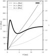 |
Fig. 2. Timescales corresponding to the Galactic frequencies f: ω, κ, and ν (left axis) and the ratio γ = 2ω/κ (right axis) as a function of Galactocentric radius R for the Allen & Santillan (1991) Galaxy model (Eq. (27)). |
The half-mass radius of the tail is the number rh, tail that fulfils
 (20)
(20)
Since the dependence of r(t, ve, α, θ, γ, κ, ν) on velocity ve is particularly simple, i.e.
 (21)
(21)
the value of rh, tail is only a function of the Galactic potential multiplied by velocity ve. This means that the time evolution of rh, tail for any  can be trivially obtained by multiplying the evolution of rh, tail calculated for one fixed value of ve by
  .
.
The dependence of rh, tail = rh, tail(t) as calculated by Eq. (22) for ve = 1 km s−1 at Galactocentric radii 6.5 kpc, 8.5 kpc, and 10.5 kpc is shown in the upper panel of Fig. 3. The extent of the tail increases non-monotonically, changing from expansion to contraction first at t ≈ 120 Myr (for R0 = 8.5 kpc), and then again starts expanding at t ≈ 180 Myr. Another tail contraction starts at t ≈ 295 Myr, so the periods of expansion are interspersed by periods of contraction.
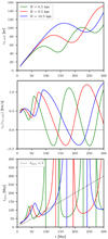 |
Fig. 3. Top panel: time dependence of the tail half-mass radius rh, tail for the semi-analytic model (Eq. (22)). Middle panel: time evolution of the mean velocity vy(rh, tail) near the radius rh, tail. The velocity oscillates substantially, and becomes negative when the tail moves towards the cluster. Lower panel: time evolution of the dynamical age of the tail, i.e. tdyn = rh, tail/vy(rh, tail). The black dotted line represents the real age tdyn = t. The dynamical age is often substantially different from the real age, making tdyn an unreliable estimate for the real age. All plots are calculated for clusters orbiting at three Galactocentric radii (6.5 kpc, green line; 8.5 kpc, red line; 10.5 kpc, blue line), and for stars escaping at velocity ve = 1 km s−1. |
It should be noted that the tail is stretched mainly in the y direction (Eq. (2.1)), so the contributions from the x and z components become unimportant as the tail stretches with time. Thus, the half-mass radius rh, tail is very close to the half-mass radius in the direction y.
The velocity near the half-mass radius vy(rh, tail) for ve = 1 km s−1 is plotted in the middle panel of Fig. 3, showing oscillations where longer intervals of tail expansion (when vy(rh, tail) > 0) are interspersed with shorter intervals of tail contraction (vy(rh, tail) < 0). This pattern is present at all the Galactocentric radii, where the value of vy(rh, tail) for clusters located closer to the inner Galaxy oscillates with a shorter period than that in the outer Galaxy. Due to the structure of Eq. (23), the velocity vy(rh, tail) for any cluster with characteristic escape speed  can be obtained by multiplying vy(rh, tail) by
  .
.
The lower panel of Fig. 3 compares the real cluster age (the dotted line) with the dynamical age of the tail tdyn, i.e. tdyn = rh, tail/vy(rh, tail) (solid lines). The dynamical age often differs by factor of ∼2 from the real cluster age, and at the time when the tail starts contracting, the dynamical time suddenly drops and even becomes negative, demonstrating that the dynamical age is rather a poor estimate for the real age.
3. Numerical methods and initial conditions
3.1. Numerical methods
The present clusters are evolved by the code NBODY6 (Aarseth 1999, 2003), which integrates trajectories of stars by the fourth-order Hermite predictor-corrector scheme (Makino 1991) with adaptive block time steps. The force acting on each star is split into its regular and irregular parts according to the Ahmad-Cohen method (Ahmad & Cohen 1973; Makino 1991). Close passages between stars and interactions in subsystems made up of two or more stars are treated by regularisation techniques (Kustaanheimo & Stiefel 1965; Aarseth & Zare 1974; Mikkola & Aarseth 1990). These sophisticated numerical methods result in a fast and very accurate code. Stellar evolution is treated by synthetic evolutionary tracks (Hurley et al. 2000) for solar metallicity.
When a star escapes the cluster, its trajectory is integrated in the external potential of the Galaxy. For the Galactic potential, we adopt the model of Allen & Santillan (1991), where the Galaxy consists of three components: the central part, disc, and halo. The potential of the central part and the disc is approximated by the Miyamoto-Nagai potential (Miyamoto & Nagai 1975),
 (22)
(22)
where i = 1 for the central part and i = 2 for the disc, and G is the gravitational constant. The Galaxy is described in cylindrical coordinates (R, z) with the origin at the Galactic centre. The central part of the Galaxy is described by parameters M1 = 1.41 × 10¹⁰ M⊙, a1 = 0, b1 = 0.387 kpc, so the model degenerates to the Plummer potential of scale-length b1. The parameters of the disc are M2 = 8.56 × 10¹⁰ M⊙, a2 = 5.32 kpc, b2 = 0.25 kpc. The potential of the dark matter halo is given by
![Mathematical equation: $$ \begin{aligned}&\phi _{3}(R) = -\frac{G M(R)}{R} - \frac{G M_3}{1.02 a_3} \times \nonumber \\&\qquad \quad \ \ \Bigg [ \left\{ \ln \left( 1 + (R_{\rm d}/a_3)^{1.02} \right) - \frac{1.02}{1 + (R_{\rm d}/a_3)^{1.02}} \right\} - \nonumber \\&\qquad \quad \ \ \left\{ \ln \left( 1 + (R/a_3)^{1.02} \right) - \frac{1.02}{1 + (R/a_3)^{1.02}} \right\} \Bigg ], \end{aligned} $$](/articles/aa/full_html/2020/08/aa36570-19/aa36570-19-eq39.gif) (23)
(23)
where
 (24)
(24)
is the halo mass inside the sphere of radius R, Rd is a radius determining the constant in the halo potential (we adopt Rd = 100 kpc), M3 = 10.7 × 10¹⁰ M⊙, and a3 = 12 kpc. The halo may be viewed as a representation of the phantom dark matter halo (Lüghausen et al. 2015). The total potential of the Galaxy is a superposition of the three potentials:
 (25)
(25)
To approximate the gas expulsion from the embedded cluster, we use the model of Kroupa et al. (2001), where the gaseous potential is given by
 (26)
(26)
Here r is the distance from the cluster centre, agas is the Plummer scale-length, and Mgas(t) is the gas mass. We choose agas to be identical to the Plummer scale-length acl for the stellar distribution. The removal of gas due to the action of newly formed stars is approximated by a decrease in the gas mass as
 (27)
(27)
where Mgas(0) is the initial mass of the gas within the cluster, td the time delay after gas expulsion commences, and τM the timescale of gas removal.
Following Kroupa et al. (2001), we adopt td = 0.6 Myr to reflect the embedded phase before gas expulsion starts, which is about the lifetime of ultra compact HII regions (Wood & Churchwell 1989; Churchwell 2002). In this work, we adopt the usual choice of gas expulsion timescale τM, which is motivated by the idea that the gas is expelled at a velocity of the order of the sound speed in ionised hydrogen: τM = agas/(10 km s−1). This means that the gas is expelled on a timescale shorter than the stellar half-mass crossing time th (impulsive gas removal), so the stellar component adjusts only slightly during the gas expulsion, and is more affected by it. In Paper II, we also explore models with τM ≫ th (adiabatic gas removal).
3.2. Initial conditions
At the beginning, the star cluster is a Plummer sphere of stellar mass Mcl and Plummer radius acl in virial equilibrium, and it is populated by stars by the method described by Aarseth et al. (1974). The stellar masses are randomly drawn from the canonical initial mass function in the form of (see Kroupa 2001; Kroupa et al. 2013),
 (28)
(28)
with the lower stellar mass limit being at the hydrogen burning limit 0.08 M⊙, and the upper stellar mass limit being at 80 M⊙, which is adopted according to the relation between the maximum mass of a star as a function of the mass of its host star cluster (Weidner et al. 2010), which we adopt to be ≈4400 M⊙ (each cluster contains 10 000 stars). Constants c1 and c2 are chosen so that the function dN/dm is continuous at 0.5 M⊙. The metallicity is close to solar, Z = 0.02. Since this is the first attempt to study the phenomenon of two tails formed by a star cluster, we do not consider primordial binary stars for the sake of simplicity. The clusters are also not primordially mass segregated. The clusters are on circular orbits of speed 220 km s−1, i.e. (vR,vϕ,vz) = (0,220,0) km s−1, at a Galactocentric distance 8.5 kpc.
4. Structure and kinematics of tail I and tail II
In order to highlight the difference between tails I and II, in this paper we adopt rather extreme models of initial conditions for star clusters. These models are not necessarily meant to reproduce the observed clusters, but the main focus is on describing the structural and kinematical differences between the two tails, and on checking the validity of the semi-analytic model. Models including other choices of parameters are studied in Paper II.
The first model (hereafter C10G13) has Mgas(0) = 2Mcl, i.e. the star formation efficiency is 33%. The Plummer scale-length acl is 0.23 pc, which is chosen according to the relation between the birth mass and the birth radius of star clusters suggested by Marks & Kroupa (2012). The other model (hereafter C10W1) is gas free, and its Plummer scale-length acl is 1 pc. We set the parameter acl for the gas-free model to be substantially larger than for the model C10G13 to have comparable half-mass radii rh for both clusters after the gas-rich model expands and revirialises due to gas expulsion (cf. Fig. 6 in Paper II).
We define the stars belonging to tail I as those that escape the cluster before the time
 (29)
(29)
where rt is the tidal radius of the cluster. The stars belonging to tail II escape after tee. The definition of tee is motivated by the fact that the stars released due to gas expulsion escape at a velocity comparable to the initial cluster velocity dispersion σcl(t = 0), so tail I is composed of stars that travel the distance to the tidal radius in a fraction (0.1) of the initial velocity dispersion. The particular value of 0.1 is implied from the shape of the velocity dispersion in the Plummer model, where the vast majority of stars move at the velocity in excess of 0.1σcl. The results are insensitive to the particular choice of the numerical factor. There are some stars that escape due to evaporation earlier than tee, and stars released due to the gas expulsion at speeds lower than 0.1σcl(t = 0) so they escape after tee, but the number of these stars is small.
The shallowing of the potential due to gas expulsion in model C10G13 unbinds 58% of its stars by time tee = 30 Myr, the escape rate then rapidly decreases, and the cluster loses 68% of its initial stellar content by 300 Myr. The evaporations and ejections alone in the gas-free model C10W1 unbind far fewer stars, only 0.3% and 5% of the total cluster population by 30 Myr and 300 Myr, respectively, so the gas expulsion model forms a tail that contains at least ten times more stars during the first ≈300 Myr of evolution.
4.1. Morphology of the tails
Figure 4 compares the morphology (left column) and velocity (right column) structure of the tidal tails of the two models. First we study the morphology. Tails I and II are depicted as blue and green dots, respectively; the tail membership is based on Eq. (29). The star cluster members are shown as red dots.
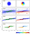 |
Fig. 4. Morphology of the tidal tails. From top to bottom: model C10G13 at 15 Myr, model C10G13 at 371 Myr (maximum thickness of tail I), model C10G13 at 406 Myr (minimum thickness of tail I), and model C10W1 at 406 Myr. Each star is represented by a coloured dot. Left column: structure of tail I (blue dots) and tail II (green dots). Members of the star cluster are shown as red dots. Right column: direction of stellar motion in the tails. The colour gives the direction of motion where the angle is measured clockwise from the unit vector pointing in the direction of positive x-axis (see the arrows in the upper middle panel and the colour bar). The cluster moves in the positive y direction around the Galaxy. |
At the beginning of the evolution of model C10G13 (t = 15 Myr; upper row), the tail expands isotropically forming approximately a sphere. This means that the escaping stars are insensitive to the variation of the Jacobi potential around the radius rt, which is in agreement with the assumption in Sect. 2 that the median escape velocity of the tail I stars ( ) is substantially higher than the potential difference at the surface of the sphere of radius rt (at |r|=rt, which is the approximate location of the Lagrange points L1 and L2), which corresponds to a velocity of ≲1 km s−1.
The second implication of the high escape speed is the large epicycle radius X (Eq. (12)), which exceeds the tidal radius rt of the cluster as the escape speed of 0.9 km s−1 implies X = 24 pc, which corresponds to the value of rt. The high escape speed also results in a substantially longer tail at a given time. Thus, the stars in tail I are brought to significantly larger or shorter Galactocentric radii than R0 ± rt forming an extended envelope around the cluster.
To illustrate the time variability of tail I found in Sect. 2, we plot the tail between its third and fourth predicted minimum of thickness (at 371 Myr; upper middle row of Fig. 4), and at the fourth predicted minimum of thickness (406 Myr; lower middle row). The tail thickness changes significantly, as does the tilt relative to the axis x = 0. The volume density close to the axis x = 0 also significantly increases near the time of the minimum thickness, facilitating the detection of the tail to a larger distance from the cluster. The minimum of tail thickness in direction x occurs almost at the time predicted in Table 1, and also the tilt x/y ≈ −0.2 is very close to the value predicted by the analytic formula.
In contrast, tail II arises gradually, at an evaporating rate nearly constant with time (Baumgardt & Makino 2003), so apart from continuing expansion from the cluster, tail II shows no tilt or oscillations of thickness (cf. the upper middle and lower middle panels). The escape speed is typically a factor of 2−3 smaller than the cluster velocity dispersion σcl. Consequently, the majority of tail II stars escape near the Lagrange points L1 and L2, where the potential barrier is the shallowest, and the slow velocity of escaping stars results in epicycle semi-minor axes X that are usually not larger than the tidal radius. Thus, for example, the stars in the trailing tail (which were released from x ≈ rt), move in the x direction mainly from x ≈ 0 to x ≈ 2rt, with few stars reaching x < 0. From symmetry, the opposite holds for the leading tail, which forms the characteristic S-shape of tail II. The morphology of tail II is almost identical to that of the tail caused by evaporating stars in the gas-free model (cf. model C10W1; last row of Fig. 4).
The relatively low escape speed of stars forming tail II results in the quadrant x > 0 and y > 0 and the quadrant x < 0 and y < 0 being practically devoid of stars (the very few stars occupying this area are mainly fast ejectors). In contrast, tail I populates these quadrants substantially (cf. the upper middle panel of Fig. 4) apart from the time near the minimum thickness. Near the events of the minimum tail thickness tx0, tail I is almost straight, while tail II is clearly S-shaped at the star cluster, and the two tails can be easily distinguished (lower middle row of Fig. 4).
4.2. Kinematics of tail stars
The right panels of Fig. 4 show the directions of motion of stars in the tail, where the colour shows the direction of motion measured from the positive x-axis clockwise, as indicated by the colourbar and the coloured arrows (for a discussion of the absolute value of the speed see Sect. 4.5). Near the beginning of the evolution, tail I expands radially (first row), and gets rotated clockwise due to the Coriolis force, gradually elongating the tail along the axis x = 0. Later (upper and upper middle plots), tail I has a shear-like motion at the time between the minima of x thickness, where the stars located at R > R0 (R0 is the radius of the cluster orbit around the Galaxy, which corresponds to x = 0) move more slowly than the cluster, and stars at R < R0 move more quickly than the cluster. The description of this movement as a shear is only an approximation; the trajectories are more complicated (cf. the arrows), where stars further away from the cluster tend to move radially (e.g. the stars in the upper panel at y ≈ −300 pc). The velocity structure of tail I changes near times tx0, where the shear-like movement transforms to an outward motion.
The majority of stars in the tail of the gas-free model C10W1 move outwards from the cluster (lower plot); the few stars moving in the opposite direction are near the cusps on their epicycles. Tail II of the gas-rich model C10G13 (upper middle and lower middle rows) is of a similar velocity structure, demonstrating that tail II is kinematically simpler than tail I.
To summarise, the trajectory of individual stars in either tail I or tail II is approximately an epicycle, but what causes the differences in the tail morphology is the value of the escape speed and the duration of the interval during which the stars escaped the cluster. The escape speed sets the semi-minor axes X of the epicycle as well as the orbital radius of the guiding centre Rg (Eqs. (7) and (12)), which determines the shape of the tail; if X ≲ rt the tail is S-shaped, if X ≳ rt the tail is extended in the x direction to several rt without being S-shaped.
4.3. Extent of the tails
The extent of the tidal tail is measured by finding the radius of a sphere centred on the cluster that contains a given fraction of the total number of stars in the tail. The stars bound to the cluster are not taken into account. These radii are analogues to the concept of Lagrangian radii. We prefer to calculate the radii for number instead of mass as we intend to avoid fluctuations due to a small number of massive stars. The evolution of the radius containing 20%, 50%, and 80% stars is shown in Fig. 5. Model C10G13 has a substantially longer tidal tail than model C10W1, measured as the tail half-number radius rh, tail; it is rh, tail = 150 pc and rh, tail = 550 pc for models C10W1 and C10G13, respectively at t = 300 Myr.
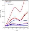 |
Fig. 5. Evolution of the 0.2, 0.5, and 0.8 Lagrangian radius of the tidal tail for the number of stars for model C10G13 (red lines) and model C10W1 (blue lines). The half-number radius is indicated by the thick lines. The dashed line represents the semi-analytical half-number radius calculated by Eq. (22) and scaled to ve = 4 km s−1, which is chosen according to the median |

The rh, tail calculated semi-analytically according to Eq. (22) and scaled by the mean escape velocity  is indicated by the dashed line. The semi-analytical model follows the direct N-body simulations well, including a close approximation to the local maximum (at ≈120 Myr) and minimum (at ≈180 Myr) of the tail extent. This implies that a good estimate for rh, tail of any cluster (e.g. a substantially more massive cluster) at any time can be obtained by multiplying the semi-analytic result of Eq. (22) (as shown in the upper panel of Fig. 3) by
  , where
  is the expected median velocity of escaping stars.
Figure 6 shows the stellar number density per 1 pc length of the tail as a function of the distance y from the cluster at selected time instants as indicated by the lines. Model C10G13 (left panel) swiftly builds a long tail. After ≈80 Myr, the density in the tail decreases only slightly with increasing |y| (the density drops only by a factor of 1.4 between y = 50 pc and y = 200 pc at t = 240 Myr), so the tail has long wings. At a given position y, the density decreases very slowly with time. In contrast, model C10W1 (right panel) builds the tidal tail very slowly, and the tail density sharply decreases outwards (the density drops by a factor of 4 between y = 50 pc and y = 200 pc at y = 240 Myr).
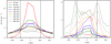 |
Fig. 6. Number density distribution of the tail as a function of the distance y along the tail for model C10G13 (left panel) and model C10W1 (right panel) at selected times as indicated by the lines. Plots at times earlier than 300 Myr (solid lines) do not indicate epicyclic overdensities. Epicyclic overdensities appear later (400−600 Myr; dotted lines). The epicyclic overdensities are located at a distance very close to the one predicted by Küpper et al. (2008), which is indicated by the vertical dashed lines. |
4.4. Epicyclic overdensities
Next we search for epicyclic overdensities in the tidal tails. Küpper et al. (2008) derive an analytic formula (their Eqs. (5) and (7)) for the distance yC of the first epicyclic overdensity from the star cluster: yC = ±2πγ(1 − γ2)rt. The formula was derived under two simplified assumptions: (i) the cluster does not gravitationally influence a star after it escapes; (ii) stars escape from the cluster with almost zero velocity. The potential adopted in this work is γ = 2ω/κ = 1.41 (cf. Fig. 2), for which yC = ±210 pc. This distance is indicated by the vertical dashed lines in Fig. 6. We note that for this potential, yC ≈ ±9rt is substantially smaller than for the Keplerian potential with γ = 2 used by Küpper et al. (2008), where yC = ±12πrt. Our models have no sign of epicyclic overdensities by the time ≈300 Myr.
Model C10W1 builds the first epicyclic overdensity at a time of 600 Myr. Model C10G13 also builds the first epicyclic overdensity after ≈400 Myr, albeit slightly closer to the cluster (around 180 pc) than in model C10W1. The positions of epicyclic overdensities, which are shown by the dashed lines, are in excellent agreement with the analytic prediction of Küpper et al. (2008). The later formation of the overdensities in model C10G13 (with respect to the work of Küpper et al. 2008, where the overdensities form at ≈2 × 2π/κ ≈ 350 Myr) might be caused by the different IMF adopted. While we use a realistic IMF, Küpper et al. (2008) assume all stars to have the same mass of 1 M⊙. The presence of relatively massive stars in our models results in mass segregation with more hard encounters between stars, which produces escapers with a broader velocity distribution and thus larger epicycle semi-minor axes X (Eq. (10)) as well as epicycles of larger loops, which smear the overdensities near the epicyclic cusps.
4.5. Bulk expansion velocity and the velocity dispersion
The mean value of the velocity vy as a function of the y distance from the cluster for the extreme models is shown in Fig. 7. Model C10G13 (left panel) has a very simple velocity structure of the tail. At a given time, the tail velocity linearly increases with cluster distance with proportionality constant ttail (i.e. vy = y/ttail). The constant ttail varies with time, changing the slope and also the sign of vy. The stars first recede from the cluster, but after ≈120 Myr, they start temporarily approaching the cluster, and at ≈215 Myr, the stars again start receding from the cluster. These events correspond to tail contraction and stretching as seen previously in Fig. 5. At a given position y, the amplitude of oscillations vy decreases with time. We note that at a given y the stars move in the shear as described in Fig. 4, but their average velocity vy is so balanced that vy always depends linearly on y.
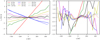 |
Fig. 7. Evolution of the bulk velocity vy of the tidal tail along the direction y at selected times as indicated by solid or dotted lines. Left panel: model C10G13. The blue dashed line indicates the analytical solution given by Eq. (19) at t = 168 Myr. Right panel: model C10W1. The vertical dashed lines represent the positions of yC according to Küpper et al. (2008). The epicyclic overdensities, which develop near the predicted positions ±240 pc at 400−600 Myr, are places where stars slow down or even reverse their motion (i.e. move towards the cluster). |
The dependence vy ∝ y closely follows the properties of Eq. (19), which is derived analytically, but which holds only at the specific times t = 2πl/κ. We plot vy according to Eq. (19) for t = 168 Myr, i.e. for l = 1 in the left panel of Fig. 7, which is shown by the dashed line. The analytical solution, which holds at t = 168 Myr, is very close to the results of the simulation which is shown at t = 160 Myr.
The tail velocity of the gas-free model C10W1 (right panel of Fig. 7) shows a clear dependence of vy ∝ y only near the cluster and at the beginning of the evolution (up to ≈120 Myr). After that time the velocity structure indicates a more complicated dependence on y. The epicyclic overdensity, which develops at ±240 pc after ≈400 Myr, can be seen as the place where the outward motion of the cluster slows or even reverses to an inward motion. We also note that the value of vy is at least a factor of 3 smaller than that of the cluster C10G13. Thus, a tail where the velocity increases as vy ∝ y/ttail to a larger distance from the cluster will point to a model strongly affected by gas expulsion. We note that the constant ttail is provided by the simulations of gas-rich clusters, and its value for clusters of different  could be obtained only by a scaling of present models.
The tail velocity dispersion  as a function of y is shown in Fig. 8. The value of σtail evolves non-monotonically with time for model C10G13 (left panel); at a given y, σtail decreases first, reaching its minimum at ≈120 Myr, and increasing afterwards. At any time, σtail shows only mild variations along |y| with a slight increase with |y|. In contrast, model C10W1 (right panel) does not show the rapid time variability in σtail. We note that the value of σtail is a factor of ≈2 larger in model C10G13 than in C10W1.
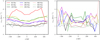 |
Fig. 8. Tail velocity dispersion σtail as a function of the distance y along the tail for model C10G13 (left panel) and model C10W1 (right panel) at selected times, as indicated by the lines. At a given position y the value of σtail evolves non-monotonically for model C10G13; it decreases first, reaching a minimum around 120 Myr, and then starts increasing. |
4.6. Minima of tail thickness and minima of the x, y, and z velocity dispersion component
After describing the characteristic properties of tail I and contrasting them with that of tail II, we turn our attention to the quantities that are intended for more direct comparison with the analytical model, namely the minima of tail thickness and velocity dispersions. These quantities are measured at the distance 200 pc < y < 300 pc from the star cluster. Model C10G13 is a good representation of tail I as these stars dominate the number of tail stars. Model C10W1 represents tail II as this model does not form tail I at all.
The thickness of the tail is plotted in Fig. 9; the left panel shows the thickness Δx in the direction x, the right panel the thickness Δz in the direction z. The thickness is an analogue to the half-number radius defined above; it is defined as the distance from the tail centre which contains 50% of the tail stars. The tail of model C10G13 (red line) shows rapid oscillations, and the times of the minima of these oscillations are in excellent agreement with the predicted minima of the analytical formulae, Eqs. (16) and (4) (thick black bars). We also note that while the minima of Δz occur periodically, the minima of Δx do not occur in periodic intervals. In contrast, the tail thickness of model C10W1 (blue line) does not oscillate periodically; apart from several spikes caused by fast ejectors, its thickness fluctuates around a constant.
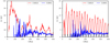 |
Fig. 9. Evolution of tail thickness Δx (left panel) and tail thickness Δz (right panel) for models C10G13 (red lines) and C10W1 (blue lines). The analysis was done at the distance 200 pc < y < 300 pc from the cluster. The predictions of the times of tail thickness minima according to Eqs. (16) and (4) are indicated by the black bars. |
The velocity structure of the tail is shown in Fig. 10. As predicted by the (semi-)analytic model, the amplitude of the velocity dispersion for tail I oscillates with time (red line in the first three plots). The minima of the velocity dispersions are again in excellent agreement with the analytic predictions (Eqs. (17), (18), and (4)). Tail II (blue line) shows no oscillations in velocity dispersions.
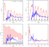 |
Fig. 10. Comparison of the tail velocity structure between models C10G13 (red lines) and C10W1 (blue lines) at 200 pc < y < 300 pc. Upper left: velocity dispersion σx. Upper right: velocity dispersion σy. Lower left: velocity dispersion σz. The minima of velocity dispersions, as calculated from Eqs. (17), (18), and (4), are indicated by the black bars. Lower right: vy component of the mean bulk tail velocity. |
The lower right panel of Fig. 10 shows the bulk velocity vy of the tail. For model C10G13, the bulk velocity oscillates from positive values of higher amplitudes to negative values of lower amplitudes. This means that the overall tail expansion changes to tail contraction; the first event of tail contraction occurs between 120 Myr and 180 Myr. We already saw the contractions in Fig. 5. In contrast, tail II of model C10W1 shows almost no oscillations. The value of |vy| is also substantially lower for model C10W1 (0.1 km s−1) than for model C10G13 (1 km s−1).
4.7. Validity of the approximation for clusters with lower velocity dispersion
One of the assumptions in finding the (semi-)analytic formulae for tail I is that the velocity dispersion, σcl, of the cluster prior to gas expulsion is significantly larger than the velocity,  , corresponding to the potential difference at the surface of the Jacobi sphere. Here we test the validity of the formulae in a non-ideal case when the assumption
  is relaxed.
For the purpose of this task, we construct additional cluster models, which are identical to model C10G13, with the exception that they have larger Plummer lengths acl and agas, and a longer gas expulsion timescale τM, which is given by τM = agas/(10 km s−1). The time delay td is again 0.6 Myr. These models are listed in Table 2.
Figure 11 contrasts the half-number radius of the tidal tail of the simulated clusters (solid lines) with the approximation of Eq. (22) (dashed lines). The models with acl ≲ 1.84 pc (σcl ≳ 3 km s−1) closely follow the semi-analytic solution. Models with acl ≳ 3.68 pc (σcl ≲ 2.1 km s−1) differ from the semi-analytic solution, but never more than by a factor of 2. Equation (22) is thus valid for  (
( is 2.2 km s−1). We note that the model without gas expulsion (C10W1), which has smaller acl than models C10G13R08 to C10G13R32, does not show the decrease in rh, tail between 120 Myr and 180 Myr followed by an increase, which is pronounced in the models with gas expulsion; the characteristic shape of the models with gas expulsion is caused by the process of gas expulsion, not by the large initial radius of these clusters.
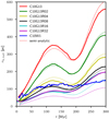 |
Fig. 11. Evolution of half-number radius of the tail for models of different values of the initial velocity dispersion (cf. Table 2). The semi-analytical solution (Eq. (22)) is plotted as dashed lines. The result of Eq. (22) is scaled to ve = 4 km s−1 for model C10G13, and then decreased by a factor of N0.5 for models labelled C10G13R“N” to scale with the initial velocity dispersion of the cluster. |
From the other major tail quantities shown in Figs. 6–10, we depict the Δx tail thickness and the bulk velocity vy for brevity (Fig. 12); the other quantities show qualitatively similar behaviour. All the models with gas expulsion show aperiodic oscillations in Δx (left panel of Fig. 12) where the amplitude of oscillation decreases with increasing acl. The minima of Δx occur close to those predicted by Eq. (16) for all the gas expulsion models, including those with  . The bulk tail velocity vy has characteristic damped oscillations for all the models with gas expulsion (right panel of Fig. 12), distinct from the evolution of vy for the model C10W1. These results indicate that all the semi-analytic formulae present in Sect. 2 are valid for any
  .
.
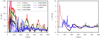 |
Fig. 12. Left panel: evolution of tail thickness Δx for models of different values of the initial velocity dispersion. The events of the minimum of tail thickness (Eq. (16)) are indicated by the black bars. Right panel: evolution of the bulk velocity vy. For clarity, we do not plot the first 80 Myr of evolution for some of the models. |
5. Conclusions
We study the morphology and kinematics of a tidal tail (tail I) formed due to a rapid release of stars from a star cluster, which orbits in a realistic gravitational potential of the Galaxy. The mechanism responsible for releasing the stars can be, for example, gas expulsion out of an embedded star cluster by stellar feedback. Tail I has distinct kinematical and morphological signatures from the more often studied tidal tails formed due to gradual dynamical evaporation or ejections (tail II), which occur throughout the cluster life-time. These signatures are studied by a (semi-)analytic model and direct simulations with the NBODY6 code. The main differences between tail I and tail II are as follows:
-
The thickness of tail I oscillates aperiodically with time in direction x and periodically in direction z (cf. Fig. 1 for orientation of the axes). The thickness varies substantially from several pc at the minima to ≈30 pc at the maxima. In contrast, the x or z thickness of tail II does not show these minima (cf. Fig. 9).
-
At the times of the minimum thickness, the narrow tail I is either parallel to the y-axis, or it is tilted by an angle ≲20° to the y-axis. When the tail is tilted, its leading part always points towards the inner Galaxy. As the tail evolves, the two types of minima thickness alternate in time with the former case (tail parallel to the y-axis) occurring for an odd minimum followed by the latter case (tail tilted to the y-axis) occurring for an even minimum.
-
The velocity dispersions in directions x, y, z also show rapid changes with time for tail I, but these quantities are non-oscillating for tail II.
-
The time events of the thickness minima, the angle of the tail relative to the y-axis, and velocity dispersion minima of tail I can be found analytically, and they very closely agree with the corresponding NBODY6 calculations. These quantities also depend only on the three galactic frequencies ω, κ, and ν, being unrelated to any property of the cluster.
-
The Lagrange radii of tail I behave non-monotonically, with longer epochs of expansion interspersed with shorter epochs of contraction. A good approximation to the evolution of the half-mass tail radius rh, tail can be found semi-analytically. The value of rh, tail at a given time is only a function of the stellar escape speed ve and Galactic frequencies ω, κ, and ν.
-
The stellar density of tail I shows only a mild decrease with |y|, so the tail has long wings (cf. Fig. 6). In contrast, the stellar density of tail II decreases sharply with |y|.
-
The velocity component vy of tail I increases linearly with the distance from the cluster, i.e. vy = y/ttail (cf. Fig. 7), where the proportionality constant ttail evolves with time (and increases in absolute value on average). In contrast, tail II has a more complicated velocity structure, particularly at later times (t ≳ 400 Myr), when epicycle overdensities develop (right panel of Fig. 7).
The semi-analytical model indicates that the different morphology and kinematics of tail I as contrasted to that of tail II is due to the two following reasons: (i) The stars of tail I leave the cluster during a short interval in comparison to the epicyclic time 2π/κ. This means that all the tail I stars have nearly the same value of κt in Eq. (2.1). This then simplifies the structure of the ensuing equations, which enables the tail x thickness and the x, y, and z component of the velocity dispersion to reach zero at distinct times. In contrast, tail II forms gradually with nearly a constant rate over several 2π/κ, so its stars have different factors κt in Eq. (2.1). (ii) The stars of tail I leave the cluster at escape velocities substantially higher than the velocity corresponding to the potential difference around the sphere of the Jacobi radius. This means that these stars escape the cluster almost isotropically, and that the sizes of their epicycle semi-minor axes are larger than the Jacobi radius. These stars thus form a tail of thickness of several Jacobi radii in the direction x, basically enveloping tail II (cf. upper middle row of Fig. 4).
In contrast, the stars in tail II leave the cluster at escape velocities usually lower than the potential difference around the sphere of the Jacobi radius. This means that these stars can escape the cluster only in the vicinity of Lagrange points L1 or L2, and that the sizes of the epicycle semi-minor axes are smaller than or comparable to that of the Jacobi radius. These stars form the relatively thin, slowly expanding, and S-shaped tail II. Numerical experiments demonstrate that all the (semi-)analytic estimates stated in the paper are valid under weaker conditions than given by the condition (ii); it is sufficient that the velocities σcl and  are comparable. This implies that the estimates hold for a larger set of initial conditions, particularly for initially less concentrated clusters.
The closer agreement between the semi-analytic model for tail I and the direct numerical simulation allows us to estimate the basic shape of the possible tail I for any Galactic star cluster on a circular orbit in the Galactic plane. For a cluster of age t on a circular orbit with given frequencies ω and κ and assuming an escape speed ve, the half-mass radius of the tail can be estimated from Eq. (22) (or upper panel of Fig. 3). These estimates are calculated for a cluster orbiting on the solar galactocentric radius 8.5 kpc and at radii 6.5 kpc and 10.5 kpc and in the plane (z = 0) of the Galactic disc. The approximate thickness of the tail could be obtained by comparing the cluster age t with the events of tail minima thickness for the cluster orbit from Eq. (16). An observational detection of tail I would strongly favour early rapid gas expulsion from the cluster with a relatively low SFE.
The present numerical study is extended by more parameters of the conditions of the early gas expulsion in Paper II, where we also provide direct predictions for the structure of the tidal tails of the Pleiades star cluster for different scenarios for the early gas expulsion.
These were referred to, respectively, as group I and group II by Kroupa et al. (2001).
Although the particular value of σcl = 8.5 km s−1 might seem substantially higher than what is observed in young star-forming regions (e.g. Kuhn et al. 2019), we adopt this example to have a testbed for the semi-analytic model with a value of  that is as high as possible. On the other hand, this model is not unreasonable because it naturally follows for an initially virialised cluster with acl = 0.23 pc. After rapid gas expulsion the velocity dispersion of the remaining cluster decreases by a factor of several, bringing it closer to the values observed in young exposed clusters (Rochau et al. 2010; Hénault-Brunet et al. 2012). Moreover, the majority of observed subclusters in star-forming regions is less massive, with a typical mass Mcl ≈ 300 M⊙ (Kuhn et al. 2015). A cluster of 300 M⊙ and acl = 0.16 pc has σcl = 2.7 km s−1, which is still higher than its
  . We also note that σcl in the present paper is the 3D velocity dispersion, which is ≈1.7× higher than the observationally accessible 1D velocity dispersion.
Acknowledgments
The authors express thanks to Sverre Aarseth for his development of the code NBODY6, which was vital for the present simulations as well as for his useful comments on the manuscript. FD would like to thank Stefanie Walch for her encouragement to work on the project while being employed within her group. FD acknowledges the support by the Collaborative Research Centre 956, sub-project C5, funded by the Deutsche Forschungsgemeinschaft (DFG) – project ID 184018867.
References
- Aarseth, S. J. 1999, PASP, 111, 1333 [NASA ADS] [CrossRef] [Google Scholar]
- Aarseth, S. J. 2003, Gravitational N-Body Simulations (Cambridge: Cambridge University Press) [Google Scholar]
- Aarseth, S. J., & Zare, K. 1974, Celest. Mech., 10, 185 [NASA ADS] [CrossRef] [Google Scholar]
- Aarseth, S. J., Henon, M., & Wielen, R. 1974, A&A, 37, 183 [NASA ADS] [Google Scholar]
- Ahmad, A., & Cohen, L. 1973, J. Comput. Phys., 12, 389 [NASA ADS] [CrossRef] [Google Scholar]
- Allen, C., & Santillan, A. 1991, Rev. Mex. Astron. Astrofis., 22, 255 [NASA ADS] [Google Scholar]
- Alves, J., Lombardi, M., & Lada, C. J. 2007, A&A, 462, L17 [NASA ADS] [CrossRef] [EDP Sciences] [Google Scholar]
- Arnold, V. I. 1989, Mathematical Methods of Classical Mechanics, 2nd ed. (New York: Springer) [Google Scholar]
- Banerjee, S., & Kroupa, P. 2013, ApJ, 764, 29 [NASA ADS] [CrossRef] [Google Scholar]
- Banerjee, S., & Kroupa, P. 2017, A&A, 597, A28 [NASA ADS] [CrossRef] [EDP Sciences] [Google Scholar]
- Bate, M. R. 2012, MNRAS, 419, 3115 [NASA ADS] [CrossRef] [Google Scholar]
- Bate, M. R. 2014, MNRAS, 442, 285 [NASA ADS] [CrossRef] [Google Scholar]
- Baumgardt, H., & Makino, J. 2003, MNRAS, 340, 227 [NASA ADS] [CrossRef] [Google Scholar]
- Baumgardt, H., & Kroupa, P. 2007, MNRAS, 380, 1589 [NASA ADS] [CrossRef] [Google Scholar]
- Baumgardt, H., De Marchi, G., & Kroupa, P. 2008, ApJ, 685, 247 [NASA ADS] [CrossRef] [Google Scholar]
- Binney, J., & Tremaine, S. 2008, Galactic Dynamics: Second Edition (Princeton University Press) [Google Scholar]
- Boily, C. M., & Kroupa, P. 2003a, MNRAS, 338, 665 [NASA ADS] [CrossRef] [Google Scholar]
- Boily, C. M., & Kroupa, P. 2003b, MNRAS, 338, 673 [NASA ADS] [CrossRef] [Google Scholar]
- Churchwell, E. 2002, ARA&A, 40, 27 [Google Scholar]
- Dale, J. E., & Bonnell, I. 2011, MNRAS, 414, 321 [NASA ADS] [CrossRef] [Google Scholar]
- Dale, J. E., Ercolano, B., & Bonnell, I. A. 2012, MNRAS, 424, 377 [NASA ADS] [CrossRef] [Google Scholar]
- De Marchi, G., Paresce, F., & Pulone, L. 2007, ApJ, 656, L65 [NASA ADS] [CrossRef] [Google Scholar]
- Dinnbier, F., & Kroupa, P. 2020, A&A, 640, A85 [EDP Sciences] [Google Scholar]
- Fujii, M. S. 2015, PASJ, 67, 59 [NASA ADS] [CrossRef] [Google Scholar]
- Fujii, M. S., & Portegies Zwart, S. 2011, Science, 334, 1380 [NASA ADS] [CrossRef] [Google Scholar]
- Fujii, M. S., & Portegies Zwart, S. 2015, MNRAS, 449, 726 [NASA ADS] [CrossRef] [Google Scholar]
- Gavagnin, E., Bleuler, A., Rosdahl, J., & Teyssier, R. 2017, MNRAS, 472, 4155 [NASA ADS] [CrossRef] [Google Scholar]
- Geyer, M. P., & Burkert, A. 2001, MNRAS, 323, 988 [NASA ADS] [CrossRef] [Google Scholar]
- Goodwin, S. P. 1997, MNRAS, 284, 785 [NASA ADS] [CrossRef] [Google Scholar]
- Goodwin, S. P., Nutter, D., Kroupa, P., Ward-Thompson, D., & Whitworth, A. P. 2008, A&A, 477, 823 [NASA ADS] [CrossRef] [EDP Sciences] [Google Scholar]
- Grudić, M. Y., Hopkins, P. F., Faucher-Giguère, C.-A., et al. 2018, MNRAS, 475, 3511 [NASA ADS] [CrossRef] [Google Scholar]
- Haid, S., Walch, S., Seifried, D., et al. 2019, MNRAS, 482, 4062 [NASA ADS] [CrossRef] [Google Scholar]
- Hénault-Brunet, V., Evans, C. J., Sana, H., et al. 2012, A&A, 546, A73 [NASA ADS] [CrossRef] [EDP Sciences] [Google Scholar]
- Hills, J. G. 1980, ApJ, 235, 986 [NASA ADS] [CrossRef] [Google Scholar]
- Hurley, J. R., Pols, O. R., & Tout, C. A. 2000, MNRAS, 315, 543 [NASA ADS] [CrossRef] [Google Scholar]
- Kroupa, P. 2001, MNRAS, 322, 231 [NASA ADS] [CrossRef] [Google Scholar]
- Kroupa, P., & Boily, C. M. 2002, MNRAS, 336, 1188 [NASA ADS] [CrossRef] [Google Scholar]
- Kroupa, P., Aarseth, S., & Hurley, J. 2001, MNRAS, 321, 699 [NASA ADS] [CrossRef] [Google Scholar]
- Kroupa, P., Weidner, C., Pflamm-Altenburg, J., et al. 2013, in The Stellar and Sub-Stellar Initial Mass Function of Simple and Composite Populations, eds. T. D. Oswalt, G. Gilmore, et al., 115 [Google Scholar]
- Kuhn, M. A., Feigelson, E. D., Getman, K. V., et al. 2014, ApJ, 787, 107 [Google Scholar]
- Kuhn, M. A., Feigelson, E. D., Getman, K. V., et al. 2015, ApJ, 812, 131 [NASA ADS] [CrossRef] [Google Scholar]
- Kuhn, M. A., Hillenbrand, L. A., Sills, A., Feigelson, E. D., & Getman, K. V. 2019, ApJ, 870, 32 [Google Scholar]
- Küpper, A. H. W., MacLeod, A., & Heggie, D. C. 2008, MNRAS, 387, 1248 [NASA ADS] [CrossRef] [Google Scholar]
- Küpper, A. H. W., Kroupa, P., Baumgardt, H., & Heggie, D. C. 2010, MNRAS, 401, 105 [NASA ADS] [CrossRef] [Google Scholar]
- Kustaanheimo, P., & Stiefel, E. 1965, Reine. Angew. Math., 218, 204 [Google Scholar]
- Lada, C. J., & Lada, E. A. 2003, ARA&A, 41, 57 [NASA ADS] [CrossRef] [Google Scholar]
- Lada, C. J., Margulis, M., & Dearborn, D. 1984, ApJ, 285, 141 [NASA ADS] [CrossRef] [Google Scholar]
- Longmore, S. N., Kruijssen, J. M. D., Bastian, N., et al. 2014, in Protostars and Planets VI, eds. H. Beuther, R. S. Klessen, C. P. Dullemond, T. Henning, et al., 291 [Google Scholar]
- Lüghausen, F., Famaey, B., & Kroupa, P. 2015, Can. J. Phys., 93, 232 [NASA ADS] [CrossRef] [Google Scholar]
- Makino, J. 1991, ApJ, 369, 200 [NASA ADS] [CrossRef] [Google Scholar]
- Marks, M., & Kroupa, P. 2012, A&A, 543, A8 [NASA ADS] [CrossRef] [EDP Sciences] [Google Scholar]
- Marks, M., Kroupa, P., & Baumgardt, H. 2008, MNRAS, 386, 2047 [NASA ADS] [CrossRef] [Google Scholar]
- Mathieu, R. D. 1983, ApJ, 267, L97 [NASA ADS] [CrossRef] [Google Scholar]
- Megeath, S. T., Gutermuth, R., Muzerolle, J., et al. 2016, AJ, 151, 5 [NASA ADS] [CrossRef] [Google Scholar]
- Mikkola, S., & Aarseth, S. J. 1990, Celest. Mech. Dyn. Astron., 47, 375 [NASA ADS] [CrossRef] [Google Scholar]
- Miyamoto, M., & Nagai, R. 1975, PASJ, 27, 533 [NASA ADS] [Google Scholar]
- Nutter, D., & Ward-Thompson, D. 2007, MNRAS, 374, 1413 [NASA ADS] [CrossRef] [Google Scholar]
- Oh, S., Kroupa, P., & Pflamm-Altenburg, J. 2015, ApJ, 805, 92 [NASA ADS] [CrossRef] [Google Scholar]
- Parmentier, G., & Gilmore, G. 2005, MNRAS, 363, 326 [NASA ADS] [CrossRef] [Google Scholar]
- Perets, H. B., & Šubr, L. 2012, ApJ, 751, 133 [NASA ADS] [CrossRef] [Google Scholar]
- Pfalzner, S. 2009, A&A, 498, L37 [NASA ADS] [CrossRef] [EDP Sciences] [Google Scholar]
- Portegies Zwart, S. F., McMillan, S. L. W., & Gieles, M. 2010, ARA&A, 48, 431 [NASA ADS] [CrossRef] [Google Scholar]
- Rochau, B., Brandner, W., Stolte, A., et al. 2010, ApJ, 716, L90 [NASA ADS] [CrossRef] [Google Scholar]
- Traficante, A., Fuller, G. A., Peretto, N., Pineda, J. E., & Molinari, S. 2015, MNRAS, 451, 3089 [NASA ADS] [CrossRef] [Google Scholar]
- Vesperini, E. 1998, MNRAS, 299, 1019 [NASA ADS] [CrossRef] [Google Scholar]
- Wall, J. E., McMillan, S. L. W., Mac Low, M.-M., Klessen, R. S., & Portegies Zwart, S. 2019, ApJ, 887, 62 [CrossRef] [Google Scholar]
- Weidner, C., Kroupa, P., & Bonnell, I. A. D. 2010, MNRAS, 401, 275 [NASA ADS] [CrossRef] [Google Scholar]
- Wood, D. O. S., & Churchwell, E. 1989, ApJS, 69, 831 [NASA ADS] [CrossRef] [Google Scholar]
- Zonoozi, A. H., Küpper, A. H. W., Baumgardt, H., et al. 2011, MNRAS, 411, 1989 [NASA ADS] [CrossRef] [Google Scholar]
All Tables
Time events when tail I thickness becomes zero (tx0; first column), and when tail I velocity dispersion in directions x and y becomes zero (tσ, x and tσ, y, respectively; third and fourth column).
All Figures
|
Fig. 1. Coordinate frame adopted for deriving the semi-analytic model of tail I. The frame is centred at the star cluster (magenta circle), and the cluster remains at rest in the frame (the frame orbits the Galaxy). The coordinate x- and y-axes, as indicated by thick black arrows, follow the usual convention where the x-axis points towards the galactic anticentre and the y-axis points in the direction of the orbit. The cluster orbits the Galactic centre at radius R0, which corresponds to x = 0 (thick blue line). The green arrow represents the initial trajectory of a star escaping the cluster. After escaping the cluster, the star moves on the red epicycle of semi-minor axis X, semi-major axis Y, and with guiding centre orbiting at Galactic radius Rg, which corresponds to x = X sin α in the adopted coordinates (thin blue line). The meaning of the escape angle α is shown by the blue curved arrow. |
| In the text | |
|
Fig. 2. Timescales corresponding to the Galactic frequencies f: ω, κ, and ν (left axis) and the ratio γ = 2ω/κ (right axis) as a function of Galactocentric radius R for the Allen & Santillan (1991) Galaxy model (Eq. (27)). |
| In the text | |
|
Fig. 3. Top panel: time dependence of the tail half-mass radius rh, tail for the semi-analytic model (Eq. (22)). Middle panel: time evolution of the mean velocity vy(rh, tail) near the radius rh, tail. The velocity oscillates substantially, and becomes negative when the tail moves towards the cluster. Lower panel: time evolution of the dynamical age of the tail, i.e. tdyn = rh, tail/vy(rh, tail). The black dotted line represents the real age tdyn = t. The dynamical age is often substantially different from the real age, making tdyn an unreliable estimate for the real age. All plots are calculated for clusters orbiting at three Galactocentric radii (6.5 kpc, green line; 8.5 kpc, red line; 10.5 kpc, blue line), and for stars escaping at velocity ve = 1 km s−1. |
| In the text | |
|
Fig. 4. Morphology of the tidal tails. From top to bottom: model C10G13 at 15 Myr, model C10G13 at 371 Myr (maximum thickness of tail I), model C10G13 at 406 Myr (minimum thickness of tail I), and model C10W1 at 406 Myr. Each star is represented by a coloured dot. Left column: structure of tail I (blue dots) and tail II (green dots). Members of the star cluster are shown as red dots. Right column: direction of stellar motion in the tails. The colour gives the direction of motion where the angle is measured clockwise from the unit vector pointing in the direction of positive x-axis (see the arrows in the upper middle panel and the colour bar). The cluster moves in the positive y direction around the Galaxy. |
| In the text | |
|
Fig. 5. Evolution of the 0.2, 0.5, and 0.8 Lagrangian radius of the tidal tail for the number of stars for model C10G13 (red lines) and model C10W1 (blue lines). The half-number radius is indicated by the thick lines. The dashed line represents the semi-analytical half-number radius calculated by Eq. (22) and scaled to ve = 4 km s−1, which is chosen according to the median |
| In the text | |
|
Fig. 6. Number density distribution of the tail as a function of the distance y along the tail for model C10G13 (left panel) and model C10W1 (right panel) at selected times as indicated by the lines. Plots at times earlier than 300 Myr (solid lines) do not indicate epicyclic overdensities. Epicyclic overdensities appear later (400−600 Myr; dotted lines). The epicyclic overdensities are located at a distance very close to the one predicted by Küpper et al. (2008), which is indicated by the vertical dashed lines. |
| In the text | |
|
Fig. 7. Evolution of the bulk velocity vy of the tidal tail along the direction y at selected times as indicated by solid or dotted lines. Left panel: model C10G13. The blue dashed line indicates the analytical solution given by Eq. (19) at t = 168 Myr. Right panel: model C10W1. The vertical dashed lines represent the positions of yC according to Küpper et al. (2008). The epicyclic overdensities, which develop near the predicted positions ±240 pc at 400−600 Myr, are places where stars slow down or even reverse their motion (i.e. move towards the cluster). |
| In the text | |
|
Fig. 8. Tail velocity dispersion σtail as a function of the distance y along the tail for model C10G13 (left panel) and model C10W1 (right panel) at selected times, as indicated by the lines. At a given position y the value of σtail evolves non-monotonically for model C10G13; it decreases first, reaching a minimum around 120 Myr, and then starts increasing. |
| In the text | |
|
Fig. 9. Evolution of tail thickness Δx (left panel) and tail thickness Δz (right panel) for models C10G13 (red lines) and C10W1 (blue lines). The analysis was done at the distance 200 pc < y < 300 pc from the cluster. The predictions of the times of tail thickness minima according to Eqs. (16) and (4) are indicated by the black bars. |
| In the text | |
|
Fig. 10. Comparison of the tail velocity structure between models C10G13 (red lines) and C10W1 (blue lines) at 200 pc < y < 300 pc. Upper left: velocity dispersion σx. Upper right: velocity dispersion σy. Lower left: velocity dispersion σz. The minima of velocity dispersions, as calculated from Eqs. (17), (18), and (4), are indicated by the black bars. Lower right: vy component of the mean bulk tail velocity. |
| In the text | |
|
Fig. 11. Evolution of half-number radius of the tail for models of different values of the initial velocity dispersion (cf. Table 2). The semi-analytical solution (Eq. (22)) is plotted as dashed lines. The result of Eq. (22) is scaled to ve = 4 km s−1 for model C10G13, and then decreased by a factor of N0.5 for models labelled C10G13R“N” to scale with the initial velocity dispersion of the cluster. |
| In the text | |
|
Fig. 12. Left panel: evolution of tail thickness Δx for models of different values of the initial velocity dispersion. The events of the minimum of tail thickness (Eq. (16)) are indicated by the black bars. Right panel: evolution of the bulk velocity vy. For clarity, we do not plot the first 80 Myr of evolution for some of the models. |
| In the text | |
Current usage metrics show cumulative count of Article Views (full-text article views including HTML views, PDF and ePub downloads, according to the available data) and Abstracts Views on Vision4Press platform.
Data correspond to usage on the plateform after 2015. The current usage metrics is available 48-96 hours after online publication and is updated daily on week days.
Initial download of the metrics may take a while.