| Issue |
A&A
Volume 639, July 2020
|
|
|---|---|---|
| Article Number | L11 | |
| Number of page(s) | 8 | |
| Section | Letters to the Editor | |
| DOI | https://doi.org/10.1051/0004-6361/202038152 | |
| Published online | 21 July 2020 | |
Letter to the Editor
Broad-line type Ic SN 2020bvc
Signatures of an off-axis gamma-ray burst afterglow
1
DARK, Niels Bohr Institute, University of Copenhagen, Lyngbyvej 2, 2100 Copenhagen, Denmark
e-mail: luca.izzo@gmail.com
2
School of Physics, The University of Melbourne, Parkville VIC 3010, Australia
3
ARC Centre of Excellence for All Sky Astrophysics in 3 Dimensions (ASTRO 3D), Sydney, Australia
4
Department of Astronomy and Astrophysics, University of California, Santa Cruz, CA 95064, USA
5
Instituto de Ciencias Nucleares, Universidad Nacional Autónoma de México, Apartado Postal 70-543, 04510 México, CDMX
Received:
12
April
2020
Accepted:
30
June
2020
Long-duration gamma-ray bursts (GRBs) are almost unequivocally associated with very energetic, broad-line supernovae of Type Ic-BL. While the gamma-ray emission is emitted in narrow jets, the SN emits radiation isotropically. Therefore, it has been hypothesized that some SN Ic-BL not associated with GRBs arise from events with inner engines such as off-axis GRBs or choked jets. Here we present observations of the nearby (d = 120 Mpc) SN 2020bvc (ASAS-SN 20bs) that support this scenario. Swift-UVOT observations reveal an early decline (up to two days after explosion), while optical spectra classify it as a SN Ic-BL with very high expansion velocities (≈70 000 km s−1), similar to that found for the jet-cocoon emission in SN 2017iuk associated with GRB 171205A. Moreover, the Swift X-Ray Telescope and CXO X-ray Observatory detected X-ray emission only three days after the SN and decaying onward, which can be ascribed to an afterglow component. Cocoon and X-ray emission are both signatures of jet-powered GRBs. In the case of SN 2020bvc, we find that the jet is off axis (by ≈23 degrees), as also indicated by the lack of early (≈1 day) X-ray emission, which explains why no coincident GRB was detected promptly or in archival data. These observations suggest that SN 2020bvc is the first orphan GRB detected through its associated SN emission.
Key words: gamma-ray burst: general / supernovae: individual: SN2020bvc / stars: jets
© ESO 2020
1. Introduction
Type Ic broad-line (BL) supernovae (SNe) form a particular class of core-collapse SNe characterized by the presence of broad absorption features (full width half maximum ≈10 000 km s−1) and extreme expansion velocities (vexp ∼ 20 000 km s−1) at the maximum of the SN emission (Modjaz et al. 2016; Gal-Yam et al. 2017). The lack of hydrogen and helium in their spectra imply that their progenitors are compact massive stars, likely Wolf-Rayet stars with initial masses M ≈ 25–30 M⊙ (Woosley & Bloom 2006) and generally characterized by low metallicity abundances (Sanders et al. 2012; Taddia et al. 2019). SNe Ic-BL are also the only flavor of SNe connected with gamma-ray bursts (GRB, Galama et al. 1998; Hjorth et al. 2003; Stanek et al. 2003; Kaneko et al. 2007), although the fraction of SNe Ic-BL associated with GRBs is only ≈10% of the entire population of SNe Ic-BL (Soderberg et al. 2006; Guetta & Della Valle 2007; Cano et al. 2017). Lack of GRB emission may be due to the presence of jet emission that is not aligned with our line of sight, given that GRB jets have average collimation angles of θ ≲ 10 deg (Frail et al. 2001; Kumar & Zhang 2015). Another possibility is that the jet is not sufficiently fed by the inner central engine such that it fails to break out of the progenitor star (the “choked-jet” scenario; MacFadyen et al. 2001; Ramirez-Ruiz et al. 2002; Lazzati et al. 2012). Extended surveys at radio frequencies have excluded the presence of off-axis jet emission in samples of SNe Ic-BL without an associated GRB (Soderberg et al. 2006; Corsi et al. 2016), although more recently for the case of the Ic-BL SN 2014ad (Stevance et al. 2017; Sahu et al. 2018) an off-axis angle of θ ≳ 30 deg could not be ruled out (Marongiu et al. 2019, but see also Ho et al. 2020a).
In the standard GRB scenario, the jet is highly collimated when it breaks out of the progenitor star. The jet opening angle is expected to be inversely related to the bulk Lorentz factor Γ of the expanding radiating plasma. This has been confirmed in theoretical (Tchekhovskoy et al. 2009; Komissarov et al. 2010) and population synthesis simulations (Ghirlanda et al. 2013). However, as the jet expands in the circumburst medium, it decelerates due to the interaction with the medium, implying a decrease in Γ and a consequent increase in the jet beaming angle (Rhoads 1997). Depending on the initial direction of the jet axis, the beaming angle of the jet will reach our line of sight at later times, which is when the afterglow starts to become visible as weak and soft X-ray emission (the “orphan” GRB afterglow; Granot et al. 2002; Kumar & Granot 2003; Piran 2005). The early interaction of the jet with the dense stellar layers of the progenitor star also gives rise to an expanding “cocoon” of material that spreads laterally with respect to the direction of the collimated jet emission (Mészáros & Rees 2001). The jet deposits a considerable amount of kinetic energy into the cocoon, which expands at mildly relativistic velocities once it breaks out of the progenitor star (Ramirez-Ruiz et al. 2002; Bromberg et al. 2011a). A choked jet, which fails to escape its progenitor star, transfers all its energy into the cocoon component (Bromberg et al. 2011b, 2012; Irwin et al. 2019). The cocoon emission is expected to be detectable a few hours after the collapse of the progenitor star (Ramirez-Ruiz et al. 2002), and once it breaks out it starts to expand into the interstellar medium. The main observational signatures for this emission are rapid (t ≈ 2–3 days) cooling, hot thermal emission, and the presence of high-velocity absorption features of Fe-peak elements in the optical spectra (Nakar & Piran 2017; Izzo et al. 2019). A considerable fraction of engine-driven SNe Ic-BL could have relativistic ejecta and could be detected at frequencies other than gamma rays. In recent years, some SNe Ic-BL have exhibited bright radio emission that can be explained with mildly relativistic velocity ejecta interacting with the circumburst medium (Soderberg et al. 2010; Margutti et al. 2014; Milisavljevic et al. 2015; Chakraborti et al. 2015). Similarly, the detection of young SNe Ic-BL can also be used to pinpoint orphan GRB afterglows, in particular at X-ray energies.
In this Letter we present the first case of an off-axis GRB discovered via its associated SN1. SN 2020bvc (or ASASSN-20bs) is a type Ic-BL SN recently discovered by the ASAS-SN survey (Shappee et al. 2014) in the nearby (d = 120 Mpc) galaxy UGC 9379. SN 2020bvc was discovered on February 4.6 2020 UT as a blue (g′ = 17 mag) rising source (Stanek 2020). The most stringent upper limit (g′ = 18.6 mag) provided by the ASAS-SN survey was obtained on February 3.6 UT, one day prior to the discovery. Spectral observations taken with the FLOYDS spectrograph at the Faulkes-North Telescope on February 5.54 UT suggested a blue featureless continuum (Hiramatsu et al. 2020), while a subsequent spectrum taken with SPRAT at the Liverpool Telescope on February 8.24 UT confirmed the type Ic-BL nature of SN 2020bvc by matching the observed spectrum with SN 1998bw six days before peak brightness (Perley et al. 2020). SN 2020bvc was detected at X-ray frequencies with the Chandra X-ray Observatory (CXO) (Ho et al. 2020b) and with the Neil Gehrels Swift Observatory (target ID = 032818, Observations 12-20). SN 2020bvc was also observed at radio frequencies (ν = 10 GHz, Fν = 63 ± 6 μJy) with the Very Large Array (VLA) (Ho et al. 2020c) on February 16.67 UT.
2. Observations
We observed SN 2020bvc with the AFOSC spectrograph, mounted on the 1.82-meter telescope of the Asiago Cima Ekar Observatory on February 28.95 UT. A series of 3 × 900 s spectra was obtained for the SN and a single spectrum for a spectrophotometric standard for the flux calibration. We reduced the data using the standard IRAF (Tody et al. 1986) procedure for long-slit spectra. The final calibrated spectrum is shown in Fig. 1, where we show the comparison with GRB-SNe 1998bw, 2003dh and 2006aj at similar epochs. The strong similarity between them confirms the type Ic-BL nature of SN 2020bvc. The position of SN 2020bvc is very close to a bright H II region of its host galaxy, UGC 9379 (Fig. 1).
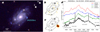 |
Fig. 1. (a) Host galaxy of SN 2020bvc, UGC 9379, as imaged by the Pan-STARRS PS1 telescope. The image was created using the g′, i′, and z′ images as single channels of an RGB image. The cyan cross gives the position of SN 2020bvc, offset 18″ from the nucleus of its host galaxy. (b, c) CXO (upper panel) and Swift-XRT (lower panel) count map image superimposed on the contours of the PS1 i-band archival image of UGC 9379. The CXO image has better spatial resolution, showing the proximity of SN 2020bvc to the H II region. (d) Spectrum of SN 2020bvc obtained with the AFOSC spectrograph at the Cima Ekar observatory in Asiago, Italy (black curve), on February 28, 2020, i.e., 24 days after the discovery of the SN, and compared with the spectra of three GRB SNe (arbitrarily offset) at similar epochs: SN 1998bw (blue: day 28, Galama et al. 1998), SN 2003dh (red: 28 days, Hjorth et al. 2003) and SN 2006aj (green: day 19, Sollerman et al. 2006). |
We extracted the Swift optical/UV light curves using a 5 arcsec aperture and the Swift analysis program UVOTSOURCE. We used a sky region of 20 arcsec radius to estimate and subtract the sky background. The UVOT magnitudes were derived assuming the most recent UVOT calibration (Breeveld et al. 2010). We did not attempt host galaxy subtraction for the Swift light curves, but the UVOT data were corrected for the Galactic extinction in the direction of SN 2020bvc, E(B − V)=0.01 mag (Schlafly & Finkbeiner 2011), using a Fitzpatrick (1999) dust extinction function. Simultaneously, SN 2020bvc was observed using the X-Ray Telescope (XRT) on board Swift. All observations were analyzed using xrtpipeline version 0.13.2, and the standard filters and screening, as suggested by the Swift data reduction guide2 and the most recent calibration database (CALDB). To place constraints on the presence of X-ray emission, we used a source region with a radius of 10 arcsec centered on the position of SN 2020bvc3 and a source-free background region with a radius of 75 arcsec located at RA = 14:34:07.0, Dec = +40:13:57.6 (J2000). In addition to the Swift-UVOT/XRT observations we also analyzed two public Directory Discretionary Time CXO observations (ObsID: 23171 and 23172; PI: Ho) of SN 2020bvc that were taken on February 16 and February 28. All data were analyzed using CIAO version 4.12 and the most recent CALDB. To extract a count rate from the CXO data, we used a source region of 2 arcsec centered on SN 2020bvc and a 20 arcsec source free background region centered at RA = 14:33:59.1, Dec = +40:15:09.9 (J2000). All extracted count rates were corrected for encircled energy fraction4. To increase the signal-to-noise ratio of the Swift-XRT observations, we merged the first two, second two, and last four observations using XSELECT version 2.4g. In all but the first epoch of the merged Swift-XRT observations, we detected faint X-ray emission arising from the position of SN 2020bvc (see Fig. 2). To convert the extracted count rates (both the 3σ upper limit and the detections), we assumed an absorbed power law with a photon index of 2, a redshift z = 0.02524 of the host galaxy of SN 2020bvc and a Galactic column density of 9.9 ×1019 cm2 along the line of sight (Ben Bekhti 2016). The UVOT and XRT light curves are shown in Fig. 2.
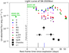 |
Fig. 2. Optical and X-ray light curve of SN 2020bvc. X-ray (Swift-XRT and CXO, 0.3–10 keV) data are plotted in black, while Swift-UVOT data are represented with colored circles (Table C.1). Zwicky Transient Facility (ZTF, Graham et al. 2019; Bellm et al. 2019) g and r data (Table C.2) are shown as triangles. We also indicate the detection and the last non-detection by the ASAS-SN survey. Time is relative to the estimated epoch of SN explosion (see Sect. 4), shown with a gray dashed line. The epochs of the FLOYDS and SPRAT spectra are shown in gray and blue. |
3. Analysis of SN 2020bvc
The UVOT light curve shows the presence of rapidly decaying UV and optical emission observed in the first three days since the SN explosion (hereafter we fix our Day 0 to February 4.0 UT, see also Sect. 4) and is characterized by fast color evolution. We built two spectral energy distributions (SEDs) using the first two epochs of UVOT data (Day 1.0 and Day 4.3 after the SN explosion, respectively). We found that these SEDs can be fitted with a thermal component with the blackbody temperature varying from T1.0 = 12 300 K to T4.3 = 6100 K (see the complete analysis in Appendix B). The radius of the thermal emitter rapidly evolves from R1.0 = (1.42 ± 0.56)×1010 km to R4.3 = (4.43 ± 1.59)×1010 km, similarly to the SN 2017iuk case (Izzo et al. 2019).
We also analyzed the FLOYDS and the SPRAT optical spectra, available from WISeREP5. The FLOYDS spectrum reveals the presence of broad absorption centered at 4300 Å and 6900 Å. We interpret these as the multiplet 42 of Fe II and the near-IR Ca II triplet at an expanding blueshifted velocity of vexp, 1 ≈ 70 000 km s−1 (see Fig. 3). These features remain visible in the later SPRAT spectrum, but with a lower expansion velocity of vexp, 2 ≈ 35 000 km s−1. The SPRAT spectrum also shows signatures of O I 7775 Å and the possible presence of Si II 6355 Å (absent in the earlier FLOYDS spectrum) at similar velocities.
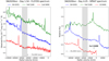 |
Fig. 3. Left panel: FLOYDS spectrum of SN 2020bvc observed one day after the SN discovery and centered on three different atomic transitions (Fe II 5169, Si II 6355, and Ca II 8490). The gray band indicates the presence of an absorption feature at vexp ≈ 70 000 km s−1, common to Fe II and Ca II, while it is not observed for Si II. Right panel: SPRAT spectrum of SN 2020bvc observed three days after the SN discovery. The red spectrum is centered on the O I 8446 line, with the position of the features indicated for a velocity of vexp ≈ 35 000 km s−1, common to Fe II and O I and barely discernible for the Si II line. |
Finally, from the analysis of the nebular emission lines visible in the Asiago spectrum, which originate from the gas surrounding the SN, we inferred the physical properties of the gas itself (see also Appendix A). We find an extinction consistent with zero, suggesting that the SN is in front of the bright underlying H II region. Moreover, using emission line indicators useful for estimating the star formation rate (SFR; Kennicutt et al. 1994) and the metallicity of the gas (i.e., the O3N2 and the N2 indices; Marino et al. 2013), we find a SFR of 0.08 M⊙ per year and a metallicity of 12 + log(O/H) = 8.16 ± 0.18. This value is consistent with the those inferred for GRB-SN host galaxies, 12 + log(O/H) = 8.22 ± 0.06 (Japelj et al. 2018; Modjaz et al. 2020).
4. Discussion
There is a striking analogy with the case of SN 2017iuk, where an early blackbody component, characterized by high-velocity absorption lines in the optical spectra, was attributed to the presence of a cocoon component originating from the jet giving rise to GRB 171205A (Izzo et al. 2019). By comparison with SN 2017iuk, we can estimate the epoch of the collapse of the massive star associated with SN 2020bvc. Considering the observed value of vexp, 1 ≈ 70 000 km s−1 on Feb 5.54 UT and the evolution of the velocity in the cocoon of SN 2017iuk, we estimate the core collapse to have happened ≈1.5 ± 0.1 days before the epoch of the FLOYDS spectrum, which results in the epoch of Feb 4.0 UT (±0.1 days) as the trigger time (Day 0) of the SN explosion.
X-ray emission from SN 2020bvc was not detected by the Swift-XRT in the first two days after the SN explosion: we report only an upper limit of FX < 3.23 × 10⁻¹⁴ erg cm−2 s−1 at the position of the SN. An increase in the X-ray emission was detected approximately three days after the discovery of the supernova. After the detection, the X-ray emission dropped following a power-law decay with a decay index α = 1.35 ± 0.09, which is consistent with the typical behavior observed in the late X-ray afterglows of GRBs (Willingale et al. 2007). The lack of a sufficient number of counts in the available X-ray observations prevents us from performing a detailed spectral analysis. However, we derive the hardness ratio HR = (H − S)/(H + S), where S and H are the number of counts in the (0.3–2) keV and (2 – 10) keV energy ranges, respectively (see Table C.3). A weighted average of the HR values gives HR = −0.66 ± 0.15, indicating a soft spectrum consistent with a photon index 1.9 < γ < 2.1, where N(ν)∝ν−γ, 6. The soft spectrum excludes a large amount of absorption, typical of interacting SNe (like that seen in Type IIn SN2010jl; Chandra et al. 2012).
We can exclude that the X-rays are associated with emission from a choked jet; in this scenario, the cocoon is composed of the shocked stellar material that expands almost isotropically after breaking out from the progenitor star (Nakar & Piran 2017). The observed emission peaks at ∼1 day, assuming an expansion velocity of ∼0.1c, and then promptly decreases, similarly to the early cooling envelope emission reported for some SNe (Nakar 2015). Instead, we have compared the total X-ray emission with simulations of an off-axis GRB afterglow light curve with the jet propagating in a stratified external medium (Granot et al. 2018, see also Fig. 5). We have found a reasonable match with the results obtained for a jet propagating at an off-axis angle of θ ≈ 23 deg within an external density profile described by a power-law density distribution as a function of the distance from the GRB progenitor R−k with the density power-law index k = 1.5, after re-scaling the theoretical curve for the distance of SN 2020bvc (d = 120 Mpc). We conclude that the X-ray emission is roughly consistent with the off-axis emission of a typical GRB with a jet energy 4 × 1050 erg, and microphysical parameters ϵe = ϵB ∼ 0.1. The hardness ratio indicates that X-ray frequencies are in the ν−p/2 part of the spectrum. Using radio observations at ∼12.7 days (Ho et al. 2020c), for the case where νm < νradio < νc < νX − rays we find that νc ∼ 6.3 × 10¹⁶ Hz for p = 2 (see Fig. 4), which is consistent with the behavior observed for GRB afterglows at late times (see, e.g., Kangas et al. 2020) and it is also consistent with the radio SED presented in Fig. 5 in Ho et al. (2020c). Alternatively, νradio < νm < νc < νX − rays, in which case we cannot set strong constraints on the value of p, although the evolution of the slow-cooling synchrotron spectrum would suggest a delayed peak in the radio emission. This last scenario opens the possibility that the early radio emission is contaminated by another component, which could be the tail of the radio cocoon emission (De Colle et al. 2018a). We also note that a good fit can be obtained with a less stratified environment and smaller observing angles (an R−2 medium is not the best choice for our models; a more detailed analysis will be presented in a future publication).
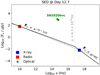 |
Fig. 4. Multi-wavelength SED computed at Day 12.7 obtained using CXO data (blue data points: this paper) and the VLA radio observations (red data points: Ho et al. 2020c). We also included the ZTF g and r data points, computed for the same epoch from interpolation of the ZTF light curve. X-ray and radio data are clearly explained within the slow-cooling afterglow scenario (black line) (Sari et al. 1998; Granot et al. 2002), with a cooling-break frequency at νc = 6.3 × 10¹⁶ Hz. The dashed gray line shows the fit results using a single power-law segment with p = 2.08. The optical data are well above the afterglow model due to the presence of the bright SN 2020bvc. |
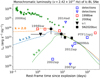 |
Fig. 5. Monochromatic (ν = 2.42 × 10¹⁷ Hz) luminosity evolution of SN 2020bvc in the first 16 days. The dashed lines represent simulations of an off-axis (θ = 23 deg) X-ray afterglow characterized by a power-law circumburst density distribution ρ ∝ R−k, with index k = 2.0 (orange), k = 1.5 (blue), and k = 0 (green). The X-ray data and upper limits of SNe Ic-BL, including SN 1998bw associated with GRB 980425, reported with squares and triangles, respectively, are from Margutti et al. (2014) and have been corrected for the (0.1–10 keV) energy range, assuming a power-law spectral model with photon index γ = 2. Also shown are the light curve of SN 2006aj associated with GRB 060218 (Campana et al. 2006). |
X-ray emission from the cocoon of a successful GRB is expected to peak a few hundred seconds after the explosion, and then to decay quickly (De Colle et al. 2018a), similarly to what is seen in SN 2017iuk (Izzo et al. 2019), thus not representing an important contribution in the emission on the observed timescale (≈days).
In Fig. 5 we compare the X-ray luminosity of SN 2020bvc with X-ray observations of low-luminosity GRB/SN, including SN 1998bw associated with GRB 980425 (Galama et al. 1998) and SN 2006 associated with GRB 060218 (Campana et al. 2006), and other SNe Ic-BL. In the sample shown in Fig. 5, SN 2020bvc is one of the brightest SNe Ic-BL observed in X-rays, similar to the luminosity of SN 1998bw, but is about one order of magnitude fainter than SN 2006aj. In this SN, the X-rays originate from a mildly-relativistic shock breakout whose luminosity and duration depend on the breakout radius rSBO (Waxman et al. 2007; Nakar 2015). For typical values of rSBO ≲ 1013 cm we should have observed an X-ray emission a few hours after the core collapse, so the lack of an X-ray detection in the first two days of the SN emission is not easily explained in the low-luminosity GRB scenario. We note that SN 2002ap was observed at similar epochs to those of SN 2020bvc, but with a much lower luminosity (≈three orders of magnitude). This was attributed to emission from shocked circumstellar matter (Soria & Kong 2002). We also note that the detection of SN 2009bb and PTF11qcj could be consistent with the simulations of an off-axis GRB afterglow (De Colle et al. 2018b). Radio observations of SN 2009bb have indeed demonstrated the presence of a bright radio afterglow, consistent with the emission from a relativistic outflow (Soderberg et al. 2010).
The jet-cocoon emission and the X-ray afterglow suggest the presence of an off-axis collimated outflow in SN 2020bvc, which was responsible for the very early optical emission and for the observed behavior of the X-ray light curve. We searched the Fermi Gamma-ray Burst Monitor (GBM) and the INTEGRAL archives for a possible gamma-ray counterpart detected by these instruments. At the expected time of the core collapse of SN 2020bvc (February 4.0 ± 0.1) we found only a sub-threshold Fermi-GBM short burst event detected on February 3.8 UT at RA, Dec = (261.220, −45.310), which is 93.71 degrees from the position of SN 2020bvc, much larger than the error radius of the GRB (r = 6.91 degrees). We also checked the Swift AFST log of observations7 at the time of the SN core collapse. Swift was pointing at several targets in this time interval, and the position of SN 2020bvc was partially covered from February 3.96 UT to February 4.08 UT, with a gap between February 4.02 and 4.04 UT. No high-energy triggers were reported by the Burst Alert Detector on board Swift. This is not surprising as the beaming angle for the gamma-ray emission is expected to be far smaller.
The analysis of the emission lines in the late spectrum of SN 2020bvc suggests a low-metallicity environment at the SN location, which is thought to be a key ingredient for the Collapsar scenario (Woosley & Bloom 2006). This is because stellar evolution at low metallicities takes place with a significantly reduced mass-loss rate during the short lifetime of the pre-SN progenitor star (Maeder & Meynet 2001) and implies faster rotating Fe cores (Izzard et al. 2004), which are expected to form jets in broad-line core-collapse SN explosions. We then conclude that SN 2020bvc represents the first orphan GRB afterglow detected through its associated SN emission, and gives further credence to the idea that a wide variety of burst phenomenology from X-ray flashes (Granot et al. 2005; Urata et al. 2015) to a fraction of low-luminosity GRBs (Ramirez-Ruiz et al. 2005) could be attributable to a relatively standard type of event being viewed from different orientations. Upcoming wide-field optical and radio surveys have the potential to detect many more (∼30–50 yr−1, Ghirlanda et al. 2015; Metzger et al. 2015) off-axis GRB afterglows and their associated SNe, which will allow us to better understand the role of jets in SNe Ic-BL.
For GRB 020410, Levan et al. (2005) used late-time (28 days) Hubble Space Telescope observations of a SN lightcurve bump to identify the GRB optical afterglow in early optical data. Similarly, for FIRST J141918.9+394036, Marcote et al. (2019) presented evidence for an off-axis afterglow on the basis of the radio emission alone.
A 10 arcsec radius corresponds to an encircled energy fraction of ∼55% at 1.5 keV assuming on-axis pointing (Moretti et al. 2004).
Acknowledgments
We thank the referee for his/her valuable comments, which definitely help to improve the quality of the paper. Based on observations collected at Copernico telescope (Asiago, Italy) of the INAF - Osservatorio Astronomico di Padova. We are grateful to P. Ochner and S. Benetti for allowing and executing the Asiago observations presented in this paper. This work was supported by a VILLUM FONDEN Investigator grant to JH (project number 16599) and by a VILLUM FONDEN Young Investigator grant to CG (project number 25501). KAA and ERR are supported by the Danish National Research Foundation (DNRF132). SIR gratefully acknowledges support from the Independent Research Fund Denmark via grant numbers DFF 4002-00275 and 8021-00130. FDC acknowledges support from UNAM-PAPIIT grant AG100820. Parts of this research were supported by the Australian Research Council Centre of Excellence for All Sky Astrophysics in 3 Dimensions (ASTRO 3D), through project number CE170100013.
References
- Arnaud, K. A. 1996, in Astronomical Data Analysis Software and Systems V, eds. G. H. Jacoby, & J. Barnes, ASP Conf. Ser., 101, 17 [Google Scholar]
- Bellm, E. C., Kulkarni, S. R., Graham, M. J., et al. 2019, PASP, 131, 018002 [NASA ADS] [CrossRef] [Google Scholar]
- Breeveld, A. A., Curran, P. A., Hoversten, E. A., et al. 2010, MNRAS, 406, 1687 [NASA ADS] [Google Scholar]
- Bromberg, O., Nakar, E., Piran, T., & Sari, R. 2011a, ApJ, 740, 100 [NASA ADS] [CrossRef] [Google Scholar]
- Bromberg, O., Nakar, E., & Piran, T. 2011b, ApJ, 739, L55 [NASA ADS] [CrossRef] [Google Scholar]
- Bromberg, O., Nakar, E., Piran, T., & Sari, R. 2012, ApJ, 749, 110 [NASA ADS] [CrossRef] [Google Scholar]
- Campana, S., Mangano, V., Blustin, A. J., et al. 2006, Nature, 442, 1008 [NASA ADS] [CrossRef] [PubMed] [Google Scholar]
- Cano, Z., Wang, S.-Q., Dai, Z.-G., & Wu, X.-F. 2017, Adv. Astron., 2017, 8929054 [NASA ADS] [CrossRef] [Google Scholar]
- Cardelli, J. A., Clayton, G. C., & Mathis, J. S. 1989, ApJ, 345, 245 [NASA ADS] [CrossRef] [Google Scholar]
- Chakraborti, S., Soderberg, A., Chomiuk, L., et al. 2015, ApJ, 805, 187 [NASA ADS] [CrossRef] [Google Scholar]
- Chandra, P., Chevalier, R. A., Irwin, C. M., et al. 2012, ApJ, 750, L2 [NASA ADS] [CrossRef] [Google Scholar]
- Corsi, A., Gal-Yam, A., Kulkarni, S. R., et al. 2016, ApJ, 830, 42 [NASA ADS] [CrossRef] [Google Scholar]
- De Colle, F., Kumar, P., & Aguilera-Dena, D. R. 2018a, ApJ, 863, 32 [NASA ADS] [CrossRef] [Google Scholar]
- De Colle, F., Lu, W., Kumar, P., Ramirez-Ruiz, E., & Smoot, G. 2018b, MNRAS, 478, 4553 [NASA ADS] [CrossRef] [Google Scholar]
- Fitzpatrick, E. L. 1999, PASP, 111, 63 [NASA ADS] [CrossRef] [Google Scholar]
- Frail, D. A., Kulkarni, S. R., Sari, R., et al. 2001, ApJ, 562, L55 [NASA ADS] [CrossRef] [Google Scholar]
- Gal-Yam, A. 2017, in Observational and Physical Classification of Supernovae, eds. W. Alsabti, & P. Murdin, 195 [Google Scholar]
- Galama, T. J., Vreeswijk, P. M., van Paradijs, J., et al. 1998, Nature, 395, 670 [NASA ADS] [CrossRef] [Google Scholar]
- Ghirlanda, G., Ghisellini, G., Salvaterra, R., et al. 2013, MNRAS, 428, 1410 [NASA ADS] [CrossRef] [EDP Sciences] [Google Scholar]
- Ghirlanda, G., Salvaterra, R., Campana, S., et al. 2015, A&A, 578, A71 [NASA ADS] [CrossRef] [EDP Sciences] [Google Scholar]
- Graham, M. J., Kulkarni, S. R., Bellm, E. C., et al. 2019, PASP, 131, 078001 [NASA ADS] [CrossRef] [Google Scholar]
- Granot, J., Panaitescu, A., Kumar, P., & Woosley, S. E. 2002, ApJ, 570, L61 [NASA ADS] [CrossRef] [Google Scholar]
- Granot, J., Ramirez-Ruiz, E., & Perna, R. 2005, ApJ, 630, 1003 [NASA ADS] [CrossRef] [Google Scholar]
- Granot, J., De Colle, F., & Ramirez-Ruiz, E. 2018, MNRAS, 481, 2711 [NASA ADS] [CrossRef] [Google Scholar]
- Guetta, D., & Della Valle, M. 2007, ApJ, 657, L73 [NASA ADS] [CrossRef] [Google Scholar]
- HI4PI Collaboration (Ben Bekhti, N., et al.) 2016, A&A, 594, A116 [NASA ADS] [CrossRef] [EDP Sciences] [Google Scholar]
- Hiramatsu, D., Arcavi, I., Burke, J., et al. 2020, Trans. Name Ser. Classification Rep., 2020–403, 1 [Google Scholar]
- Hjorth, J., Sollerman, J., Møller, P., et al. 2003, Nature, 423, 847 [NASA ADS] [CrossRef] [PubMed] [Google Scholar]
- Ho, A. Y. Q., Corsi, A., Cenko, S. B., et al. 2020a, ApJ, 893, 132 [CrossRef] [Google Scholar]
- Ho, A. Y. Q., Cenko, B., Perley, D., Corsi, A., & Brightman, M. 2020b, Trans. Name Ser. AstroNote, 45, 1 [Google Scholar]
- Ho, A. Y. Q., Kulkarni, S. R., Perley, D. A., et al. 2020c, ApJ, submitted [arXiv:2004.10406] [Google Scholar]
- Irwin, C. M., Nakar, E., & Piran, T. 2019, MNRAS, 489, 2844 [NASA ADS] [CrossRef] [Google Scholar]
- Izzard, R. G., Ramirez-Ruiz, E., & Tout, C. A. 2004, MNRAS, 348, 1215 [NASA ADS] [CrossRef] [Google Scholar]
- Izzo, L., de Ugarte Postigo, A., Maeda, K., et al. 2019, Nature, 565, 324 [Google Scholar]
- Japelj, J., Vergani, S. D., Salvaterra, R., et al. 2018, A&A, 617, A105 [NASA ADS] [CrossRef] [EDP Sciences] [Google Scholar]
- Kaneko, Y., Ramirez-Ruiz, E., Granot, J., et al. 2007, ApJ, 654, 385 [NASA ADS] [CrossRef] [Google Scholar]
- Kangas, T., Fruchter, A. S., Cenko, S. B., et al. 2020, ApJ, 894, 43 [CrossRef] [Google Scholar]
- Kennicutt, Jr., R. C., Tamblyn, P., & Congdon, C. E. 1994, ApJ, 435, 22 [Google Scholar]
- Komissarov, S. S., Vlahakis, N., & Königl, A. 2010, MNRAS, 407, 17 [NASA ADS] [CrossRef] [Google Scholar]
- Kumar, P., & Granot, J. 2003, ApJ, 591, 1075 [CrossRef] [Google Scholar]
- Kumar, P., & Zhang, B. 2015, Phys. Rep., 561, 1 [NASA ADS] [CrossRef] [Google Scholar]
- Lazzati, D., Morsony, B. J., Blackwell, C. H., & Begelman, M. C. 2012, ApJ, 750, 68 [NASA ADS] [CrossRef] [Google Scholar]
- Levan, A., Nugent, P., Fruchter, A., et al. 2005, ApJ, 624, 880 [NASA ADS] [CrossRef] [Google Scholar]
- MacFadyen, A. I., Woosley, S. E., & Heger, A. 2001, ApJ, 550, 410 [NASA ADS] [CrossRef] [Google Scholar]
- Maeder, A., & Meynet, G. 2001, A&A, 373, 555 [NASA ADS] [CrossRef] [EDP Sciences] [Google Scholar]
- Marcote, B., Nimmo, K., Salafia, O. S., et al. 2019, ApJ, 876, L14 [NASA ADS] [CrossRef] [Google Scholar]
- Margutti, R., Milisavljevic, D., Soderberg, A. M., et al. 2014, ApJ, 797, 107 [NASA ADS] [CrossRef] [Google Scholar]
- Marino, R. A., Rosales-Ortega, F. F., Sánchez, S. F., et al. 2013, A&A, 559, A114 [NASA ADS] [CrossRef] [EDP Sciences] [Google Scholar]
- Marongiu, M., Guidorzi, C., Margutti, R., et al. 2019, ApJ, 879, 89 [NASA ADS] [CrossRef] [Google Scholar]
- Mészáros, P., & Rees, M. J. 2001, ApJ, 556, L37 [NASA ADS] [CrossRef] [Google Scholar]
- Metzger, B. D., Williams, P. K. G., & Berger, E. 2015, ApJ, 806, 224 [NASA ADS] [CrossRef] [Google Scholar]
- Milisavljevic, D., Margutti, R., Parrent, J. T., et al. 2015, ApJ, 799, 51 [NASA ADS] [CrossRef] [Google Scholar]
- Modjaz, M., Liu, Y. Q., Bianco, F. B., & Graur, O. 2016, ApJ, 832, 108 [NASA ADS] [CrossRef] [Google Scholar]
- Modjaz, M., Bianco, F. B., Siwek, M., et al. 2020, ApJ, 892, 153 [CrossRef] [Google Scholar]
- Moretti, A., Campana, S., Tagliaferri, G., et al. 2004, in SWIFT XRT Point Spread Function Measured at the Panter End-to-end Tests, eds. K. A. Flanagan, & O. H. W. Siegmund, SPIE Conf. Ser., 5165, 232 [NASA ADS] [Google Scholar]
- Nakar, E. 2015, ApJ, 807, 172 [Google Scholar]
- Nakar, E., & Piran, T. 2017, ApJ, 834, 28 [NASA ADS] [CrossRef] [Google Scholar]
- Osterbrock, D. E., & Ferland, G. J. 2006, Astrophysics of Gaseous Nebulae and Active Galactic Nuclei [Google Scholar]
- Perley, D., Schulze, S., & Bruch, R. 2020, Trans. Name Server AstroNote, 37, 1 [Google Scholar]
- Piran, T. 2005, Rev. Mod. Phys., 76, 1143 [Google Scholar]
- Ramirez-Ruiz, E., Celotti, A., & Rees, M. J. 2002, MNRAS, 337, 1349 [NASA ADS] [CrossRef] [Google Scholar]
- Ramirez-Ruiz, E., Granot, J., Kouveliotou, C., et al. 2005, ApJ, 625, L91 [NASA ADS] [CrossRef] [Google Scholar]
- Rhoads, J. E. 1997, ApJ, 487, L1 [NASA ADS] [CrossRef] [Google Scholar]
- Sahu, D. K., Anupama, G. C., Chakradhari, N. K., et al. 2018, MNRAS, 475, 2591 [NASA ADS] [CrossRef] [Google Scholar]
- Sanders, N. E., Soderberg, A. M., Levesque, E. M., et al. 2012, ApJ, 758, 132 [NASA ADS] [CrossRef] [Google Scholar]
- Sari, R., Piran, T., & Narayan, R. 1998, ApJ, 497, L17 [NASA ADS] [CrossRef] [Google Scholar]
- Schlafly, E. F., & Finkbeiner, D. P. 2011, ApJ, 737, 103 [NASA ADS] [CrossRef] [Google Scholar]
- Shappee, B. J., Prieto, J. L., Grupe, D., et al. 2014, ApJ, 788, 48 [NASA ADS] [CrossRef] [Google Scholar]
- Soderberg, A. M., Nakar, E., Berger, E., & Kulkarni, S. R. 2006, ApJ, 638, 930 [NASA ADS] [CrossRef] [PubMed] [Google Scholar]
- Soderberg, A. M., Chakraborti, S., Pignata, G., et al. 2010, Nature, 463, 513 [NASA ADS] [CrossRef] [Google Scholar]
- Sollerman, J., Jaunsen, A. O., Fynbo, J. P. U., et al. 2006, A&A, 454, 503 [NASA ADS] [CrossRef] [EDP Sciences] [Google Scholar]
- Soria, R., & Kong, A. K. H. 2002, ApJ, 572, L33 [NASA ADS] [CrossRef] [Google Scholar]
- Stanek, K. Z. 2020, Trans. Name Server Discovery Rep., 2020–381, 1 [Google Scholar]
- Stanek, K. Z., Matheson, T., Garnavich, P. M., et al. 2003, ApJ, 591, L17 [NASA ADS] [CrossRef] [Google Scholar]
- Stevance, H. F., Maund, J. R., Baade, D., et al. 2017, MNRAS, 469, 1897 [NASA ADS] [CrossRef] [Google Scholar]
- Taddia, F., Sollerman, J., Fremling, C., et al. 2019, A&A, 621, A71 [NASA ADS] [CrossRef] [EDP Sciences] [Google Scholar]
- Tchekhovskoy, A., McKinney, J. C., & Narayan, R. 2009, ApJ, 699, 1789 [NASA ADS] [CrossRef] [Google Scholar]
- Tody, D. 1986, in The IRAF Data Reduction and Analysis System, ed. D. L. Crawford, SPIE Conf. Ser., 627, 733 [NASA ADS] [Google Scholar]
- Urata, Y., Huang, K., Yamazaki, R., & Sakamoto, T. 2015, ApJ, 806, 222 [NASA ADS] [CrossRef] [Google Scholar]
- Waxman, E., Mészáros, P., & Campana, S. 2007, ApJ, 667, 351 [NASA ADS] [CrossRef] [Google Scholar]
- Willingale, R., O’Brien, P. T., Osborne, J. P., et al. 2007, ApJ, 662, 1093 [NASA ADS] [CrossRef] [Google Scholar]
- Woosley, S. E., & Bloom, J. S. 2006, ARA&A, 44, 507 [NASA ADS] [CrossRef] [Google Scholar]
Appendix A: Local environment of SN 2020bvc
We investigated the physical properties of the gas surrounding the location of SN 2020bvc from an analysis of the nebular emission lines visible in the spectrum. We clearly detect Balmer lines (Hα, Hβ, Hγ), the [O III] 4959,5007 Å lines, and a very faint [N II] 6584 Å line. We report the fluxes of these lines in Table A.1. From an analysis of the Balmer lines we estimated the local extinction using the Balmer decrement ratio. The observed ratio (Hα/Hβ)obs = 2.88 ± 0.22 is consistent with the theoretical value of (Hα/Hβ)th = 2.86 obtained from a typical H II temperature of T = 10 000 K and an electron density ne = 102 cm−3 for Case B recombination (Osterbrock & Ferland 2006). This suggests that the SN is located in front of the bright H II region in UGC 9379 and, in particular, it suggests a local extinction consistent with zero: E(B − V)int = 0.01 ± 0.01 mag. From the luminosity of the Hα line we estimated the SFR using the Kennicutt et al. (1994) formulation; from an inferred luminosity of L = 1.08 × 1040 erg s−1, we obtain a SFR of 0.08 M⊙ per year. Finally, we estimated the gas metallicity using the emission line ratio indicators N2 and O3N2 in the formulation provided by Marino et al. (2013). Using the values reported in Table A.1, we obtain 12 + log(O/H) = 8.16 ± 0.18 using the O3N2 indicator and 12 + log(O/H) = 8.36 ± 0.16 using the N2 indicator. The values obtained from the N2 and O3N2 indicators are consistent within their uncertainties. If we use the O3N2 value, the metallicity inferred for the SN 2020bvc environment is consistent with the value inferred for GRB-SNe host galaxies, 12 + log(O/H) = 8.22 ± 0.06 (Japelj et al. 2018; Modjaz et al. 2020).
Observed fluxes for the nebular emission lines measured in the Asiago spectrum of SN 2020bvc.
Appendix B: SED analysis
We used the Swift-UVOT observations to build two SEDs at the earliest epochs in order to constrain the temperature and radius of the thermal emitter observed in the first days of the SN 2020bvc emission. We also included the g- and r-band ZTF observations that are closest in time to each SED epoch in order to extend the UV and optical wavelength range from ∼2000 Å to ∼7000 Å. We used Swift data observed at MJD = 58884.0 and MJD = 58887.3 (see also Table C.1) that have been complemented with ZTF data observed on MJD = 58884.5 and MJD = 58887.5, respectively (see also Table C.2). The two datasets were fit using a blackbody model and two absorption models that take into account the Galactic interstellar reddening (E(B − V)=0.039 mag) and an additional model that corrects for the dust grain extinction in the host galaxy, with the E(B − V) parameter fixed to the value of 0.01 mag obtained from the Balmer decrement ratio analysis. For both models we used a Cardelli et al. (1989) extinction law. The fits were obtained using XSPEC (Arnaud 1996) and the results are shown in Table B.1 (see also Fig. B.1). The normalization term is proportional to the luminosity of the thermal component, from which we estimated the radius R of the emitter using the equation relating the luminosity from a blackbody with its radius and temperature T,
with σ being the Stefan–Boltzmann constant. We assume a distance to SN 2020bvc of d = 120 Mpc.
Best-fit results obtained for the SEDs built using Swift and ZTF data on MJD = 58884.0 and MJD = 58887.3.
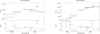 |
Fig. B.1. Swift and ZTF data of SN 2020bvc obtained on MJD = 58884.0 (left panel) and MJD = 58887.3 (right panel) with the best-fit results obtained using an absorbed blackbody model (see text). |
Appendix C: Data tables
Swift-UVOT data.
Data for ZTF (Graham et al. 2019; Bellm et al. 2019) and ASAS-SN (Shappee et al. 2014).
Swift-XRT and CXO data.
All Tables
Observed fluxes for the nebular emission lines measured in the Asiago spectrum of SN 2020bvc.
Best-fit results obtained for the SEDs built using Swift and ZTF data on MJD = 58884.0 and MJD = 58887.3.
Data for ZTF (Graham et al. 2019; Bellm et al. 2019) and ASAS-SN (Shappee et al. 2014).
All Figures
|
Fig. 1. (a) Host galaxy of SN 2020bvc, UGC 9379, as imaged by the Pan-STARRS PS1 telescope. The image was created using the g′, i′, and z′ images as single channels of an RGB image. The cyan cross gives the position of SN 2020bvc, offset 18″ from the nucleus of its host galaxy. (b, c) CXO (upper panel) and Swift-XRT (lower panel) count map image superimposed on the contours of the PS1 i-band archival image of UGC 9379. The CXO image has better spatial resolution, showing the proximity of SN 2020bvc to the H II region. (d) Spectrum of SN 2020bvc obtained with the AFOSC spectrograph at the Cima Ekar observatory in Asiago, Italy (black curve), on February 28, 2020, i.e., 24 days after the discovery of the SN, and compared with the spectra of three GRB SNe (arbitrarily offset) at similar epochs: SN 1998bw (blue: day 28, Galama et al. 1998), SN 2003dh (red: 28 days, Hjorth et al. 2003) and SN 2006aj (green: day 19, Sollerman et al. 2006). |
| In the text | |
|
Fig. 2. Optical and X-ray light curve of SN 2020bvc. X-ray (Swift-XRT and CXO, 0.3–10 keV) data are plotted in black, while Swift-UVOT data are represented with colored circles (Table C.1). Zwicky Transient Facility (ZTF, Graham et al. 2019; Bellm et al. 2019) g and r data (Table C.2) are shown as triangles. We also indicate the detection and the last non-detection by the ASAS-SN survey. Time is relative to the estimated epoch of SN explosion (see Sect. 4), shown with a gray dashed line. The epochs of the FLOYDS and SPRAT spectra are shown in gray and blue. |
| In the text | |
|
Fig. 3. Left panel: FLOYDS spectrum of SN 2020bvc observed one day after the SN discovery and centered on three different atomic transitions (Fe II 5169, Si II 6355, and Ca II 8490). The gray band indicates the presence of an absorption feature at vexp ≈ 70 000 km s−1, common to Fe II and Ca II, while it is not observed for Si II. Right panel: SPRAT spectrum of SN 2020bvc observed three days after the SN discovery. The red spectrum is centered on the O I 8446 line, with the position of the features indicated for a velocity of vexp ≈ 35 000 km s−1, common to Fe II and O I and barely discernible for the Si II line. |
| In the text | |
|
Fig. 4. Multi-wavelength SED computed at Day 12.7 obtained using CXO data (blue data points: this paper) and the VLA radio observations (red data points: Ho et al. 2020c). We also included the ZTF g and r data points, computed for the same epoch from interpolation of the ZTF light curve. X-ray and radio data are clearly explained within the slow-cooling afterglow scenario (black line) (Sari et al. 1998; Granot et al. 2002), with a cooling-break frequency at νc = 6.3 × 10¹⁶ Hz. The dashed gray line shows the fit results using a single power-law segment with p = 2.08. The optical data are well above the afterglow model due to the presence of the bright SN 2020bvc. |
| In the text | |
|
Fig. 5. Monochromatic (ν = 2.42 × 10¹⁷ Hz) luminosity evolution of SN 2020bvc in the first 16 days. The dashed lines represent simulations of an off-axis (θ = 23 deg) X-ray afterglow characterized by a power-law circumburst density distribution ρ ∝ R−k, with index k = 2.0 (orange), k = 1.5 (blue), and k = 0 (green). The X-ray data and upper limits of SNe Ic-BL, including SN 1998bw associated with GRB 980425, reported with squares and triangles, respectively, are from Margutti et al. (2014) and have been corrected for the (0.1–10 keV) energy range, assuming a power-law spectral model with photon index γ = 2. Also shown are the light curve of SN 2006aj associated with GRB 060218 (Campana et al. 2006). |
| In the text | |
|
Fig. B.1. Swift and ZTF data of SN 2020bvc obtained on MJD = 58884.0 (left panel) and MJD = 58887.3 (right panel) with the best-fit results obtained using an absorbed blackbody model (see text). |
| In the text | |
Current usage metrics show cumulative count of Article Views (full-text article views including HTML views, PDF and ePub downloads, according to the available data) and Abstracts Views on Vision4Press platform.
Data correspond to usage on the plateform after 2015. The current usage metrics is available 48-96 hours after online publication and is updated daily on week days.
Initial download of the metrics may take a while.