| Issue |
A&A
Volume 639, July 2020
|
|
|---|---|---|
| Article Number | A126 | |
| Number of page(s) | 8 | |
| Section | Stellar structure and evolution | |
| DOI | https://doi.org/10.1051/0004-6361/202037966 | |
| Published online | 21 July 2020 | |
A strong neutron burst in jet-like supernovae of spinstars
1
Department of Physics, Faculty of Science and Engineering, Konan University, 8-9-1 Okamoto, Kobe, Hyogo 658-8501, Japan
e-mail: This email address is being protected from spambots. You need JavaScript enabled to view it.
2
Geneva Observatory, University of Geneva, Maillettes 51, 1290 Sauverny, Switzerland
3
Kavli Institute for the Physics and Mathematics of the Universe (WPI), The University of Tokyo, 5-1-5 Kashiwanoha, Kashiwa, Chiba 277-8583, Japan
4
Department of Physics and Astronomy, Clemson University, Clemson, SC 29634-0978, USA
Received:
16
March
2020
Accepted:
28
May
2020
Abstract
Context. Some metal-poor stars have abundance patterns, which are midway between the slow (s) and rapid (r) neutron capture processes.
Aims. We show that the helium shell of a fast rotating massive star experiencing a jet-like explosion undergoes two efficient neutron capture processes: one during stellar evolution and one during the explosion. It eventually provides a material whose chemical composition is midway between the s- and r-process.
Methods. A low metallicity 40 M⊙ model with an initial rotational velocity of ∼700 km s−1 was computed from birth to pre-supernova with an extended nuclear network following the slow neutron capture process. A two-dimensional hydrodynamic relativistic code was used to model a E = 1052 erg relativistic jet-like explosion hitting the stellar mantle. The jet-induced nucleosynthesis was calculated in post-processing with an optimised network of 1812 nuclei.
Results. During the star’s life, heavy elements from 30 ≲ Z ≲ 82 are produced thanks to an efficient s-process, which is boosted by rotation. At the end of evolution, the helium shell is largely enriched in trans-iron elements and in (unburnt) 22Ne, whose abundance is ∼20 times higher than in a non-rotating model. During the explosion, the jet heats the helium shell up to ∼1.5 GK. It efficiently activates (α, n) reactions, such as 22Ne(α, n), and leads to a strong n-process with neutron densities of ∼1019 − 1020 cm−3 during 0.1 s. This has the effect of shifting the s-process pattern, which was built during stellar evolution, towards heavier elements (e.g. Eu). The resulting chemical pattern is consistent with the abundances of the carbon-enhanced metal-poor r/s star CS29528-028, provided the ejecta of the jet model is not homogeneously mixed.
Conclusions. The helium burning zones of rotating massive stars experience an efficient s-process during the evolution followed by an efficient n-process during a jet-like explosion. This is a new astrophysical site which can explain at least some of the metal-poor stars showing abundance patterns midway between the s- and r-process.
Key words: stars: massive / stars: rotation / stars: jets / stars: interiors / nuclear reactions, nucleosynthesis, abundances
© ESO 2020
1. Introduction
Understanding the origin of the elements is among the very topical challenges of modern astrophysics (e.g. the reviews of Meyer 1994; Arnould et al. 2007; Thielemann et al. 2017; Cowan et al. 2019; Arnould & Goriely 2020). The solar abundances first revealed the existence of a slow (s) and a rapid (r) neutron capture process (Suess & Urey 1956; Burbidge et al. 1957). The s-process operates during the life of asymptotic giant branch (AGB, main s-process, e.g. Busso et al. 1999; Herwig 2005; Lugaro et al. 2012; Karakas & Lattanzio 2014) and massive stars (weak s-process, e.g. Langer et al. 1989; Prantzos et al. 1990; Käppeler et al. 2011). Promising sites for the r-process include neutron star mergers (e.g. Wanajo et al. 2014; Thielemann et al. 2017) as well as magneto-rotational supernovae and collapsars from massive stars (e.g. Winteler et al. 2012; Nishimura et al. 2015; Halevi & Mösta 2018; Siegel et al. 2019).
Besides the Sun, metal-poor (MP) stars (e.g. the review of Beers & Christlieb 2005; Frebel & Norris 2015) are prime targets to investigate the origin of elements since they likely formed from a material that was enriched by just one or a few previous sources. Thus their abundances only reflect one or a few previous nucleosynthetic events. A zoo of MP stars was progressively constituted based on the chemical composition of these objects. Numerous MP stars have supersolar [C/Fe] ratios and are called carbon-enhanced metal-poor (CEMP) stars. At [Fe/H] ≲ − 3, most MP stars are CEMP stars and generally do not show clear enhancements in heavy elements (CEMP-no stars, e.g. Yong et al. 2013; Norris et al. 2013; Bonifacio et al. 2015; Yoon et al. 2016). In addition to carbon, most CEMP-no stars have supersolar [N/Fe], [O/Fe], [Na/Fe], [Mg/Fe], and [Al/Fe] ratios. The most discussed scenarios to explain these nearly pristine objects that are enriched in light elements rely on massive stellar models experiencing significant mixing at the time of the supernova and possibly strong fallback (e.g. Umeda & Nomoto 2003; Limongi et al. 2003; Nomoto et al. 2003; Iwamoto et al. 2005; Heger & Woosley 2010; Tominaga et al. 2007b, 2014; Ishigaki et al. 2018) and models experiencing mid to fast rotation during their lives (e.g. Meynet et al. 2006, 2010; Hirschi 2007; Joggerst et al. 2010; Maeder et al. 2015; Takahashi et al. 2014; Choplin et al. 2017a, 2019).
At [Fe/H] ≳ − 3, many CEMP stars with clear enhancement of heavy elements were found. This includes CEMP stars with clear s-process signatures (CEMP-s stars, e.g. Burris et al. 2000; Simmerer et al. 2004; Sivarani et al. 2004; Placco et al. 2013) and r-process signatures (CEMP-r stars, e.g. Sneden et al. 2003; Ji et al. 2016; Hansen et al. 2018; Sakari et al. 2018). The origin of the CEMP-r stars is tightly linked to the r-process site (cf. first paragraph). Most of the CEMP-s stars are found in binary systems (Hansen et al. 2016) and are thought to have acquired their s-processed material, from a now extinct AGB companion, during a (wind) mass transfer episode (e.g. Stancliffe & Glebbeek 2008; Bisterzo et al. 2010; Masseron et al. 2010; Lugaro et al. 2012; Hollek et al. 2015; Abate et al. 2015). An efficient s-process is also expected in rotating massive stars (cf. Sect. 2) and therefore these objects could explain at least a part of the CEMP-s sample (Choplin et al. 2017b; Banerjee et al. 2019). In addition to CEMP-s and CEMP-r stars, one also finds r +s CEMP stars, which are likely made of a combination of s- and r-process patterns (Gull et al. 2018), and CEMP-r/s stars (also named CEMP-i stars, e.g. Roederer et al. 2016). This last class shows intermediate abundance patterns for which neither an s-process nor an r-process pattern, and likely nor a combination of both, can reasonably reproduce the abundances (Jonsell et al. 2006; Lugaro et al. 2012; Bisterzo et al. 2012; Abate et al. 2016). An intermediate neutron capture process, that is, an i-process operating at neutron densities in between the s- and r-process (first named by Cowan & Rose 1977), may be a solution to explain these stars1 (Dardelet et al. 2014; Roederer et al. 2016; Hampel et al. 2016, 2019). The i-process may operate in AGB or super-AGB stars (Herwig et al. 2011; Jones et al. 2017) in rapidly accreting white dwarfs (Denissenkov et al. 2017, 2019) or in the helium shell of very low (or zero) metallicity massive stars experiencing proton ingestion events during late evolutionary stages (Banerjee et al. 2018; Clarkson et al. 2018).
In addition to the s-, r-, and i-processes, one finds the n-process. It consists in a short neutron burst in the helium shell of massive stars when the supernova shock wave passes through it (Blake & Schramm 1976; Truran et al. 1978; Thielemann et al. 1979; Blake et al. 1981; Hillebrandt et al. 1981; Rauscher et al. 2002; Meyer et al. 2004). Most of the neutron are provided by the 22Ne(α,n) reaction. It has been shown that the n-process could explain some anomalous isotopic signatures in meteorites (Meyer et al. 2000; Pignatari et al. 2015, 2018).
Here, we propose a new scenario providing abundance patterns midway between the s- and r-process and which can possibly explain the metal-poor stars having these types of intermediate abundance patterns. This scenario relies on two successive neutron capture processes in the same source: an efficient s-process followed by a strong n-process. The basic working of it is explained in Sect. 2. The codes used and methods are presented in Sect. 3, the results and comparisons with the metal-poor star C29528-028 are presented in Sects. 4 and 5, respectively, followed by discussions in Sect. 6. A summary and the main conclusions are given in Sect. 7.
2. The helium shell of a rotating massive star hit by a jet
This section describes the basic working of the scenario discussed throughout this paper. By progressively transporting chemical elements from a burning region to another rotational mixing impacts the nucleosynthesis during stellar evolution (e.g. Meynet & Maeder 2000; Heger et al. 2000; Brott et al. 2011; Chieffi & Limongi 2013; Choplin et al. 2016). Especially, rotation has been found to increase the production of 13C and 22Ne, which release neutrons by (α, n) reactions. It boosts the efficiency of the s-process in massive stars, mainly during the core helium burning stage (Pignatari et al. 2008; Frischknecht et al. 2012, 2016; Limongi & Chieffi 2018; Choplin et al. 2018; Banerjee et al. 2019, see also Sect. 4.1).
As mentioned in Sect. 1, at the time of the supernova, the shock wave passing through the helium shell can trigger the n-process. Its efficiency very much depends on the pre-supernova amount of 22Ne and the ability of the explosion to burn it during the shock passage. In case of a rotating progenitor, the n-process can be particularly efficient. On the one hand, rotation produces more 22Ne during the evolution and allows for a higher amount of unburnt 22Ne in the helium shell at the pre-supernova stage. On the other hand, rotation may trigger energetic jet-like explosions (e.g. Woosley 1993; MacFadyen & Woosley 1999; Woosley & Heger 2006), thus leading to high temperatures in the helium shell and therefore an efficient activation of the 22Ne(α, n) reaction.
The combined effect of fast rotation and jet-like explosion can induce an efficient s-process during evolution and an efficient n-process during explosion. In this paper we examine the combination of these two effects.
3. Methods
We modelled the evolution and explosion of a 40 M⊙ star by combining a one-dimensional stellar evolution code with a two-dimensional explosion code. The Geneva stellar evolution code (Eggenberger et al. 2008) was used to compute a pre-supernova 40 M⊙ model at a metallicity of Z = 10−3 with an initial rotation rate on the zero-age main sequence of υini/υcrit = 0.82. This corresponds to an initial equatorial velocity of 704 km s−1. The nuclear network was coupled to the evolution and used throughout the entire process. It comprises 737 isotopes from hydrogen to polonium. We refer to Choplin & Hirschi (2020) for more details on the initial set up of the model.
The jet-like explosion was modelled with a two-dimensional relativistic hydrodynamical code (Tominaga et al. 2007a; Tominaga 2009). At t = 0, a jet was launched at the mass coordinate 1.93 M⊙, lasting for 10 seconds with a constant energy deposition rate of 1051 erg s−1. The total energy deposited is then 1052 erg, which corresponds to the typical energy of a hypernova (e.g. Nomoto et al. 2004, 2006). The opening angle is 5 degrees and the Lorentz factor is Γ = 100. The hydrodynamics is followed for 5 × 10⁵ s. The thermodynamic histories are recorded by 2.5 × 10⁴ mass particles representing Lagrangian mass elements of the stellar mantle. The initial grid is linear with a resolution of 100 along the θ-direction and logarithmic with a resolution of 250 in the r-direction. The nucleosynthesis of mass particles initially located in the helium shell was calculated in post-processing with a neutron-rich nuclear network of 1812 isotopes. Nucleosynthesis tests with different network sizes were carried out in order to reduce the network size as much as possible without missing isotopes.
4. Results
During its life, this rotating 40 M⊙ model loses 16 M⊙ through stellar winds: 8% of the mass is lost during the main sequence, 82% during core helium burning, and 10% after core helium burning. The final mass of the model is then Mfin = 24 M⊙ with a hydrogen envelope that is mainly composed of helium (71% in mass). The final surface hydrogen mass fraction is 0.3 (Fig. 1) and the total hydrogen mass left in the star is 1.4 M⊙. For comparison purposes, the same model without rotation loses 6.42 M⊙, has a final hydrogen envelope of 18.29 M⊙ (composed of ∼45% hydrogen and ∼55% helium), has a final surface hydrogen mass fraction of 0.73, and the total hydrogen mass that is left in the star is 8.2 M⊙.
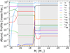 |
Fig. 1. Pre-supernova abundance profile of the rotating 40 M⊙ progenitor model. The outer layers are shown. The shaded areas show the convective zones. |
4.1. Rotation-induced nucleosynthesis during stellar evolution
We recall below how rotation boosts the s-process during the evolution of massive stars (cf. discussions in Pignatari et al. 2008; Frischknecht et al. 2016; Limongi & Chieffi 2018; Choplin et al. 2018; Banerjee et al. 2019). During the core helium burning phase, 12C and 16O are transported by rotation-induced mixing from the helium core to the hydrogen shell, which boosts the CNO cycle in the hydrogen shell and synthesises primary313C and 14N. Due to the growth of the convective helium core combined with the backward diffusion of hydrogen burning products, the extra 13C and 14N are engulfed in the helium core The 14N is quickly transformed into 22Ne through 14N(α, γ)18F(β+)18O(α, γ)22Ne. Neutrons, which are mainly released by 13C(α, n) and 22Ne(α, n), trigger the s-process provided any heavy seed (e.g. 56Fe) is present in the helium burning core.
In the present model, this effect boosts the s-process by a factor of ∼10 − 1000 for elements with 35 < Z < 82 (Fig. 2). The same model without rotation only experiences a modest enhancement of elements with Z < 45 (Fig. 2, black line). At the pre-supernova stage, the mass fraction of 22Ne that is left (unburnt) in the helium shell is 2.2 × 10⁻² (Fig. 1), which is ∼20 times higher than for the same model but without rotation.
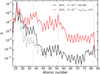 |
Fig. 2. Integrated mass fractions of the material above the bottom of the helium shell (after beta decays) at the pre-supernova stage. The red (black) solid line shows a low metallicity 40 M⊙ model computed with (without) rotation. The black dashed line shows the initial chemical composition of the models. The vertical dotted lines show the location of Sr, Ba, and Pb. |
4.2. Jet-induced nucleosynthesis: Light elements
The jet penetrates into the helium shell after 2 s. The mass particles located at the bottom of the helium shell have pre-jet temperatures of 0.3 − 0.4 GK. Those with θini ≤ 10° reach 1 < T < 1.5 GK during the passage of the jet (Fig. 3).
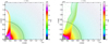 |
Fig. 3. Location of the mass particles after 2.8 s (left panel) and 5.4 s (right panel). The colour shows the temperature of the mass particles. The inner grey circle shows the central remnant. The black circle with a radius of ∼0.7 × 1010 cm shows the location of the bottom of the helium shell. |
Close to the jet axis, the high temperature activates 22Ne(α, n), but also 13C(α, n) and 17O(α, n), the isotopes 13C and 17O being produced by 12C(n, γ) and 16O(n, γ) (Fig. 4). Even closer to the jet axis and deeper in the helium shell, the higher temperature efficiently produces 24Mg, 28Si, and 32S (Fig. 5) through (α, γ) reactions. Some (α, p) reactions, such as 24Mg(α, p)27Al and 27Mg(α, p)30Si, also become strong and, therefore, they release protons, which activate some (p, γ) reactions. For instance, 31P is enhanced (Fig. 5) through 30Si(p, γ)31P. The high 35Cl abundance comes from the chain 24Mg(α, p)27Al(α, p)30Si(α, γ)34S(p, γ)35Cl. The high 36Ar and 39K mainly come from 34S(p, γ)35Cl(p, γ)36Ar and 34S(α, γ)38Ar(p, γ)39K, respectively. Some Ti is also formed thanks to 44Ca(p, γ)45Sc(p, γ)46Ti.
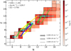 |
Fig. 4. Flowchart of a mass particle with Mr, ini = 16.53 M⊙ (i.e. originally in the helium shell, cf. Fig. 1) and θini = 3.15° at its temperature peak. Mass fractions of isotopes are shown by the red colourmap. Black squares denote stable isotopes. Net reaction rates, considering forward and reverse reactions, are shown by arrows. Arrows are coloured as a function of the reaction type: yellow for (α, γ), cyan for (n, γ), green for (α, n), and blue for (γ, α) and (n, α). Rates below 7 × 1022 cm s−1 are not shown. |
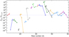 |
Fig. 5. Effect of the jet on C−Ti elements for a mass particle with Mr, ini = 15.78 M⊙ and θini = 0.45°. We note that Xjet are the post-jet mass fractions and Xno jet are the mass fractions of the same mass particle that would not have experienced a jet explosion. In both cases, elements are beta decayed. |
4.3. Jet-induced nucleosynthesis: Heavy elements
During the jet explosion, the (α, n) reactions lead to a burst of neutrons. For mass particles that are initially along the jet axis (θini ≲ 5°) and with initial mass coordinates of Mr, ini ∼ 15.5 − 18 M⊙, the neutron density reaches nn > 1019 cm−3 during ∼0.1 s (Fig. 7, left panel). The neutron exposure4 of these mass particles goes up to 1.35 mbarn−1 (Fig. 7). Despite nn values being close to r-process values, the abundant light elements in the helium shell (especially 12C and 16O) act as strong neutron poisons. This reduces the amount of available neutron for heavy seeds and does not lead to r-process nucleosynthesis. Nevertheless, during the burst, isotopes that are far from the valley of stability are produced (Fig. 8, bottom panel). The pre-jet abundance pattern is therefore shifted towards higher mass numbers compared to the initial pattern (Fig. 9). In particular, the first (A ∼ 80 − 90) and second (A ∼ 130 − 140) s-process peaks that were built during stellar evolution are shifted to higher atomic masses (see also Fig. 6). Details on the nucleosynthesis are given below.
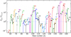 |
Fig. 6. Same as Fig. 5, but for Fe−Ho elements and for a mass particle with Mr, ini = 16.53 M⊙ and θini = 3.15° (same mass particle as in Fig. 4). |
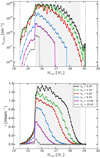 |
Fig. 7. Maximum neutron density (top) and neutron exposure (bottom) during the jet explosion as a function of the initial mass coordinate. Coloured lines show different initial angles. Each point represents a mass particle with initial coordinates θini and Mr, ini. The two dashed lines show the initial location of the bottom of helium and hydrogen shells. The shaded areas show the convective zone at the pre-jet stage (see also Fig. 1). |
 |
Fig. 8. Pre-jet mass fractions (top panel) and post-jet mass fractions (before beta decays, bottom panel) for a mass particle at Mr, ini = 16.53 M⊙ and θini = 3.15° (same mass particle as in Fig. 4). Black squares denote stable isotopes. The light blue line shows a typical r-process flow for comparison purposes (taken from Arnould & Goriely 2020, their Fig. 5). The grey line shows the neutron drip line. Thin dotted lines show the location of the magic numbers. |
During the jet explosion, 56, 57, 58, 60Fe are mostly transformed into 60 − 64Fe by neutron captures. After the explosion, 60 − 64Fe eventually decay to the stable 60, 61, 62, 64Ni and 63Cu isotopes. This has the overall effect of destroying Fe and somewhat increasing Ni and Cu (Figs. 6 and 10). The 59Co isotope, which is the only stable isotope of Co, is mainly transformed into 62 − 69Co isotopes which decay to Ni, Cu, Zn, and 69Ga. The production of 59Fe, 59Mn, and 59Cr, which will decay to 59Co, is too small to replenish 59Co and therefore the final Co abundance stays low (Fig. 10). The higher final Zn abundance is mainly due to the decay of 66, 67, 68Ni to 66, 67, 68Zn isotopes. The final Mo is also enhanced, mainly thanks to the decay of neutron-rich Zr (96 − 100Zr) isotopes to stable Mo isotopes. The final Ru is enhanced thanks to the decay of the neutron-rich Zr (101, 102, 104Zr), Nb, and Mo isotopes to stable Ru isotopes. We note that 103Rh, which is the only stable isotope of Rh, is largely enhanced by the decay of 103Zr, 103Nb, and 103Mo. It is similar for Nd, Sm, Eu, Gd, Tb, and Dy (Z = 60 − 66) elements whose final abundances are raised (Figs. 6 and 10) because of the decays of the neutron-rich isotopes of Cs, Ba, La, Ce, and Pr (Z = 55 − 59). The final Tm, Lu, and Ta abundances are lower because they experience efficient neutron captures until the neutron magic number 126 (Fig. 8), and they are not efficiently replenished by neutron-rich isotopes for elements with a lower atomic mass. For instance, most of the initial 169 − 173Tm are transformed into 195Tm, which eventually decay to 195Pt, and Tm is only slightly replenished by the decay of 169Sm, 169Eu, and 169Gd, whose post-jet mass fractions are small (about 10−11). The abundance of 209Bi also increases (Fig. 10) because of the decay of the unstable 209Tl and 209Pb isotopes, which are produced during the jet explosion. Furthermore, Pb is not affected by the jet explosion because of a closed loop of beta and alpha decays leading back to Pb (or possibly 209Bi). For instance, any unstable 210Pb produced during the explosion experiences double beta decay to 210Po, and then alpha decay to the stable 206Pb isotope.
The stable isotopes, which are shielded by isotopes with the same mass and a lower atomic number, are not replenished by beta decays and are therefore completely destroyed by the jet. This is the case for 136Ba or 148Sm (Fig. 6) whose final mass fractions are nearly zero because they are shielded by the stable 136Xe and 148Nd isotopes, respectively.
4.4. Case of a spherical explosion
As a test, we ran two spherical explosions: one with the same total energy (ETOT = 1052 erg) and one with ETOT = 1053 erg. For the 1052 erg spherical explosion, the bottom of the helium shell is heated up to ∼0.6 GK. In this case, the (α, n) reactions are weaker and the neutron density goes up to ∼1015 cm−3. It leads to a much smaller neutron exposure that slightly affects the distribution of heavy elements. For a 1053 erg spherical explosion, the bottom of the helium shell is heated up to ∼1 GK, which leads to a maximal neutron density of about ∼1019 − 20 cm−3, that is, similar to the jet-explosion discussed throughout this paper. In this case, the abundances of heavy elements are significantly affected in the same way as in Figs. 9 and 10. This means that ≳10 times more energetic spherical explosions could lead to a similar nucleosynthesis as the 1052 erg jet-like explosion considered in this work. We note that a 1053 erg explosion corresponds to an extreme case which may not be realistic5. Consequently, the nucleosynthetic signature of a boosted n-process (as discussed throughout this paper) very likely points towards jet-like, or at least aspherical, explosions. We plan to explore the effect of various opening angles and explosion energies in a future work.
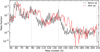 |
Fig. 9. Pre-jet and post-jet mass fractions for the mass particle at Mr, ini = 16.53 M⊙ and θini = 3.15° (the same mass particle as in Figs. 1, 4, and 8). The vertical dotted lines show the location of 88Sr, 138Ba, and 208Pb. |
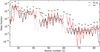 |
Fig. 10. Effect of the jet on heavy elements for the mass particle at Mr, ini = 16.53 M⊙ and θini = 3.15° (the same mass particle as in Figs. 1, 4, 8, and 9). The solid red line shows the composition after the jet explosion and after beta decays. The solid black line shows the composition if no jet explosion occurred (still after beta decays). Dashed lines show the patterns before beta decays. |
5. Signature in the metal-poor star CS29528-028
The chemical signature of jet-like explosions from rotating stars may be seen at the surface of observed metal-poor stars that have formed with the material ejected by previous sources. Here, we focus on CS29528-028 which has [Fe/H] −2.12, Teff = 7100 K, and log g = 4.27 (Allen et al. 2012). It was classified as a carbon-enhanced metal-poor star with heavy abundances midway between the s- and r-process (CEMP-r/sBeers & Christlieb 2005) because of its high [C/Fe] = 2.76, enrichment in trans-Fe elements, and intermediate [Ba/Eu] = 0.33 (Aoki et al. 2007; Allen et al. 2012). Aoki et al. (2007) reported a [Na/Fe] ratio of 2.68, but with a suggested NLTE correction of −0.7, thus giving [Na/Fe]NLTE = 1.98.
We compared the abundances of CS29528-028 with four models. The first and second ones are 40 M⊙ non-rotating and rotating models, respectively, which did not experience jet-induced nucleosynthesis (orange and black lines in Fig. 11). The mass cut was set at a mass coordinate of 1.93 M⊙ (just as the jet model, cf. Sect. 3). The ejecta of the non-rotating (rotating) model was mixed with 150 (400) M⊙ of ISM material to produce the fits shown in Fig. 11. The third model (rot+jet_A, blue pattern) shows the integrated chemical composition of all ejected mass particles after the jet. For the fourth model, we searched for the best fit by considering the dependance of the yields in the final angle θfin and final velocity vfin of the ejected material. Indeed, a neighbouring halo hosting a future star may not be enriched by the full ejecta, but only by a part of it, having a certain angle range. Also, the higher velocity material is more likely to reach and enrich a neighbouring halo. The rot+jet_B model (red pattern in Fig. 11) shows the best fit when the final angle range and the velocity threshold vth are left as free parameters; it is important to specify that only the mass particles with vfin > vth were considered in this case. This model corresponds to the integration of the mass particles with 7 < θfin < 17° and with vfin > 0.04 c. The mass particles in this angle range are located in between the two dashed lines shown in Fig. 12. The mass particles with vfin > 0.04 c are enclosed by the outermost contour shown in Fig. 12.
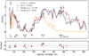 |
Fig. 11. Best fits (top panel) and their residuals (bottom panel) for the metal-poor star CS29528-028. The squares are the abundances from Aoki et al. (2007), and the circles are from Allen et al. (2012). Only an upper limit was derived for nitrogen. When two measurements were available for one element, the most recent one (Allen et al. 2012) was selected to calculate χ2 and used to plot the residuals. The four patterns show the best fits and their χ2 value for four models (cf. text for details). All models were considered after beta decay. |
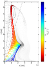 |
Fig. 12. Location of the mass particles at t = 5 × 10⁵ s. The coloured particles represent the particles originally in the helium shell. The colourmap shows the initial angles of these particles. The two dashed lines show θ = 7 and 17°. Iso-velocity contours are shown for particles that have the highest velocities (vfin > 0.04 c). Lighter contours correspond to higher velocities. |
Without rotation, the enrichment in elements with Z > 40 cannot be reproduced. Rotation provides elements from the second s-process peak but lacks Nd and Eu. Jet-induced nucleosynthesis boosts the production of the elements beyond the first and second s-process peaks (cf. Sect. 4.3) and, therefore, can provide the required Nd and Eu (rot+jet_B model). However, if the ejecta is fully mixed (rot+jet_A model), Nd and Eu are underproduced. This is because in this case the material processed by the jet is diluted with a large amount of unprocessed (or slightly processed) material, which blurs the nucleosynthesis signature of the jet.
The rot+jet_B model requires that the fastest ejecta in a given angle range reaches a nearby halo hosting the future CS29528-028 star. The requirements of this scenario are stringent, meaning that it may be a rare event.
6. Discussion
6.1. The efficiency of the n-process
First, the strength of the n-process very much depends on the amount of 22Ne in the helium-shell at the pre-SN stage. In a non-rotating model, this amount is directly linked to the initial amount of CNO elements: During the main-sequence, the CNO cycle transforms most of the initial CNO into 14N and the 14N is converted into 22Ne during helium burning by the chain 14N(α, γ)18F(β+)18O(α, γ)22Ne. Therefore, higher metallicity stars, which contain more CNO at birth, are more likely to experience a more efficient n-process. At solar metallicity, the initial sum of CNO elements in a mass fraction is about 10−2, which leads to a 22Ne mass fraction at the pre-SN stage of about 10−2 at maximum. This is similar to the case discussed here (Fig. 1), meaning that an energetic explosion at solar metallicity should also lead to an efficient n-process.
Rotation-induced mixing synthesises additional primary 22Ne during the core-helium burning phase (cf. Sect. 4.1). Some of it is burnt during the evolution, thus boosting the s-process, and some of it is left at the pre-SN stage. If the leftover 22Ne is burnt during the explosion, that boosts the n-process. Rotation can therefore provide a significant amount of 22Ne at the pre-SN stage, even at low metallicity, and thus leads to a boosted n-process at low metallicity.
Nevertheless, the n-process scales with the abundances of existing heavy seeds (e.g. Fe, Sr, Ba) in the helium shell at the pre-SN stage. This process merely redistributes the abundances of heavy elements in the helium shell. If the abundances of the heavy seed are very small in the shell at the pre-SN stage, the n-process continues to operate but the absolute abundances of heavy elements stay very small.
Finally, the strength of the n-process is highly dependent on the peak temperature reached in the helium-shell during the explosion. It the peak temperature is too low, the 22Ne(α, n) reaction is not efficiently activated and the n-process stays weak, regardless of the pre-SN 22Ne abundance. For a given energy, an aspherical explosion allows for a higher peak temperature to be reached in the helium shell (cf. Sect. 4.4).
For instance, Rauscher et al. (2002) reported that for non-rotating solar metallicity ∼20 M⊙ stars exploding as spherical type II SNe with 1051 ≲ E ≲ 2 × 1051 erg, the n-process only slightly redistributes the heavy elements at the bottom of the helium shell (cf. their section 5.4). These models contain 22Ne, but it is likely not significantly burnt during the explosion.
6.2. The n- and the i-process
In the nuclear chart, the boosted n-process that is studied here populates a region midway between the s-process and r-process regions (Fig. 8). However, this process differs from the i-process. The latter is associated with hydrogen ingestion in a convective helium burning region, which triggers the chain 12C(p, γ)13N(β+)13C(α, n) and leads to neutron densities in between the s- and r-process (typically nn ∼ 1013 cm−3–1015 cm−3, Cowan & Rose 1977; Malaney 1986; Dardelet et al. 2014; Clarkson et al. 2018; Denissenkov et al. 2019; Hampel et al. 2019). Typical neutron exposures are 1 ≲ τ ≲ 20 mbarn−1 and the timescale involved is ≳1 day. By contrast, in the case of the n-process, the neutrons are mainly provided by the 22Ne(α, n) reaction; the timescale is shorter (∼1 s) because of the explosive nature of the event. Also, the neutron density is higher and the neutron exposure is similar or lower (Fig. 7).
6.3. On the production of Pb in massive stars
The abundance of Pb is challenging to determine in metal-poor stars because it generally relies on a single line, which may be blended by a CH line. Although Pb is not detected in CS29528-028, some CEMP-r/s stars have a high Pb abundance (e.g. Placco et al. 2013).
We recall that any Pb that is synthesised during the massive star evolution in the helium shell should not be affected by the passage of the jet (cf. Sect. 4.3). Thus, if any Pb is synthesised in massive stars, it should occur during stellar evolution. The rotating massive stellar models of Limongi & Chieffi (2018) and Banerjee et al. (2019) produce a significant amount of Pb during their lives, while only small or modest amounts are synthesised in similar models from Frischknecht et al. (2012, 2016), Choplin et al. (2018), Choplin & Hirschi (2020), and from this work (cf. Fig 2). Among the important parameters impacting the production of Pb is the treatment of rotation in the stellar interior, which varies from code to code. An efficient internal rotational mixing during stellar evolution favours the production of Pb: It provides more 22Ne and 13C (cf. Sect. 2) and thus increases the neutron source (13C, 22Ne) over seed (e.g. 56Fe) ratio, thus boosting the production of heavier s-elements, such as Pb. Unfortunately, the physics of rotation still suffers from important uncertainties and therefore a firm answer cannot be given now.
7. Summary and conclusions
We inspected the combined effect of fast rotation and jet-like explosion on the helium shell nucleosynthesis of a low metallicity 40 M⊙ star. As has already been found, rotation boosts the s-process during the evolution and leaves a high amount of unprocessed 22Ne in the helium shell at the pre-supernova stage. An energetic jet-like explosion heats the helium shell up to ∼1.5 GK. It efficiently activates (α, n) reactions (especially 22Ne(α, n)) and leads to neutron densities of 1019 − 1020 cm−3 for ∼0.1 s. This neutron burst shifts the s-process pattern towards heavier elements. In particular, the production of Mo, Ru, and Rh (right after the first s-process peak) and Nd, Sm, Eu, and Gb (right after the second s-process peaks) is significantly boosted. A spherical explosion, with the energy equally distributed to all angles, does not heat the helium shell sufficiently enough to produce these types of high neutron densities unless the explosion energies is extremely high, about 1053 erg.
Overall we have shown that the helium shell of a rotating massive star experiences two successive efficient neutron capture processes: an efficient s-process during the evolution and an efficient n-process during a jet-like explosion. It gives a material whose chemical composition is midway between the s- and r-process. Such a scenario may explain the metal-poor stars showing these types of intermediate abundance patterns. In particular, the abundances of the CEMP-r/s star CS29528-028 are compatible with the yields of our jet model, provided a non-homogeneous mixing of the ejecta.
We also note that the r-process may occur in the jet or accretion disc of jet-like explosions (e.g. Winteler et al. 2012; Nishimura et al. 2015; Siegel et al. 2019). Depending on the degree of mixing between the jet, disc, and stellar mantle material, combinations of s-, n-, and r-process patterns may result and produce a variety of chemical signatures in the interstellar medium.
Such a process has also been proposed to explain the isotopic signature of presolar grains (Jadhav et al. 2013; Liu et al. 2014).
The initial equatorial velocity is υini and υcrit is the initial equatorial velocity at which the gravitational acceleration is balanced by the centrifugal force. It is defined as 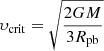 , where Rpb is the polar radius at the break-up velocity (see Maeder & Meynet 2000).
Produced from the initial hydrogen and helium content of the star, but not from the initial metals.
The neutron exposure was computed as 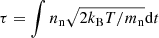 with nn the neutron density, kB the Boltzmann constant, T the temperature, and mn the neutron mass.
The strongest explosions detected have 1052 < E < 1053 erg (see e.g. Fig. 2 in Nomoto et al. 2013).
Acknowledgments
The authors thank an anonymous referee for constructive comments that improved the manuscript. A.C. acknowledges funding from the Swiss National Science Foundation under grant P2GEP2_184492. B.S.M. acknowledges funding from NASA Grant NNX17AE32G.
References
- Abate, C., Pols, O. R., Izzard, R. G., & Karakas, A. I. 2015, A&A, 581, A22 [NASA ADS] [CrossRef] [EDP Sciences] [Google Scholar]
- Abate, C., Stancliffe, R. J., & Liu, Z.-W. 2016, A&A, 587, A50 [NASA ADS] [CrossRef] [EDP Sciences] [Google Scholar]
- Allen, D. M., Ryan, S. G., Rossi, S., Beers, T. C., & Tsangarides, S. A. 2012, A&A, 548, A34 [NASA ADS] [CrossRef] [EDP Sciences] [Google Scholar]
- Aoki, W., Beers, T. C., Christlieb, N., et al. 2007, ApJ, 655, 492 [NASA ADS] [CrossRef] [Google Scholar]
- Arnould, M., & Goriely, S. 2020, Progress in Particle and Nuclear Physics, 112, 103766 [NASA ADS] [CrossRef] [Google Scholar]
- Arnould, M., Goriely, S., & Takahashi, K. 2007, Phy. Rep., 450, 97 [Google Scholar]
- Banerjee, P., Qian, Y.-Z., & Heger, A. 2018, ApJ, 865, 120 [NASA ADS] [CrossRef] [Google Scholar]
- Banerjee, P., Heger, A., & Qian, Y.-Z. 2019, ApJ, 887, 187 [Google Scholar]
- Beers, T. C., & Christlieb, N. 2005, ARA&A, 43, 531 [NASA ADS] [CrossRef] [Google Scholar]
- Bisterzo, S., Gallino, R., Straniero, O., Cristallo, S., & Käppeler, F. 2010, MNRAS, 404, 1529 [NASA ADS] [Google Scholar]
- Bisterzo, S., Gallino, R., Straniero, O., Cristallo, S., & Käppeler, F. 2012, MNRAS, 422, 849 [NASA ADS] [CrossRef] [Google Scholar]
- Blake, J. B., & Schramm, D. N. 1976, ApJ, 209, 846 [NASA ADS] [CrossRef] [EDP Sciences] [Google Scholar]
- Blake, J. B., Woosley, S. E., Weaver, T. A., & Schramm, D. N. 1981, ApJ, 248, 315 [NASA ADS] [CrossRef] [Google Scholar]
- Bonifacio, P., Caffau, E., Spite, M., et al. 2015, A&A, 579, A28 [NASA ADS] [CrossRef] [EDP Sciences] [Google Scholar]
- Brott, I., de Mink, S. E., Cantiello, M., et al. 2011, A&A, 530, A115 [NASA ADS] [CrossRef] [EDP Sciences] [Google Scholar]
- Burbidge, E. M., Burbidge, G. R., Fowler, W. A., & Hoyle, F. 1957, Rev. Mod. Phys., 29, 547 [NASA ADS] [CrossRef] [Google Scholar]
- Burris, D. L., Pilachowski, C. A., Armandroff, T. E., et al. 2000, ApJ, 544, 302 [NASA ADS] [CrossRef] [Google Scholar]
- Busso, M., Gallino, R., & Wasserburg, G. J. 1999, ARA&A, 37, 239 [NASA ADS] [CrossRef] [Google Scholar]
- Chieffi, A., & Limongi, M. 2013, ApJ, 764, 21 [NASA ADS] [CrossRef] [Google Scholar]
- Choplin, A., & Hirschi, R. 2020, ArXiv e-prints [arXiv:2001.02341] [Google Scholar]
- Choplin, A., Maeder, A., Meynet, G., & Chiappini, C. 2016, A&A, 593, A36 [NASA ADS] [CrossRef] [EDP Sciences] [Google Scholar]
- Choplin, A., Ekström, S., Meynet, G., et al. 2017a, A&A, 605, A63 [NASA ADS] [CrossRef] [EDP Sciences] [Google Scholar]
- Choplin, A., Hirschi, R., Meynet, G., & Ekström, S. 2017b, A&A, 607, L3 [NASA ADS] [CrossRef] [EDP Sciences] [Google Scholar]
- Choplin, A., Hirschi, R., Meynet, G., et al. 2018, A&A, 618, A133 [NASA ADS] [CrossRef] [EDP Sciences] [Google Scholar]
- Choplin, A., Tominaga, N., & Ishigaki, M. N. 2019, A&A, 632, A62 [CrossRef] [EDP Sciences] [Google Scholar]
- Clarkson, O., Herwig, F., & Pignatari, M. 2018, MNRAS, 474, L37 [NASA ADS] [CrossRef] [Google Scholar]
- Cowan, J. J., & Rose, W. K. 1977, ApJ, 212, 149 [NASA ADS] [CrossRef] [Google Scholar]
- Cowan, J. J., Sneden, C., Lawler, J. E., et al. 2019, ArXiv e-prints [arXiv:1901.01410] [Google Scholar]
- Dardelet, L., Ritter, C., Prado, P., et al. 2014, XIII Nuclei in the Cosmos (NIC XIII), 145 [Google Scholar]
- Denissenkov, P. A., Herwig, F., Battino, U., et al. 2017, ApJ, 834, L10 [NASA ADS] [CrossRef] [Google Scholar]
- Denissenkov, P. A., Herwig, F., Woodward, P., et al. 2019, MNRAS, 488, 4258 [CrossRef] [Google Scholar]
- Eggenberger, P., Meynet, G., Maeder, A., et al. 2008, Ap&SS, 316, 43 [NASA ADS] [CrossRef] [Google Scholar]
- Frebel, A., & Norris, J. E. 2015, ARA&A, 53, 631 [NASA ADS] [CrossRef] [Google Scholar]
- Frischknecht, U., Hirschi, R., & Thielemann, F.-K. 2012, A&A, 538, L2 [NASA ADS] [CrossRef] [EDP Sciences] [Google Scholar]
- Frischknecht, U., Hirschi, R., Pignatari, M., et al. 2016, MNRAS, 456, 1803 [NASA ADS] [CrossRef] [Google Scholar]
- Gull, M., Frebel, A., Cain, M. G., et al. 2018, ApJ, 862, 174 [NASA ADS] [CrossRef] [Google Scholar]
- Halevi, G., & Mösta, P. 2018, MNRAS, 477, 2366 [NASA ADS] [CrossRef] [Google Scholar]
- Hampel, M., Stancliffe, R. J., Lugaro, M., & Meyer, B. S. 2016, ApJ, 831, 171 [NASA ADS] [CrossRef] [Google Scholar]
- Hampel, M., Karakas, A. I., Stancliffe, R. J., Meyer, B. S., & Lugaro, M. 2019, ApJ, 887, 11 [NASA ADS] [CrossRef] [Google Scholar]
- Hansen, T. T., Andersen, J., Nordström, B., et al. 2016, A&A, 588, A3 [NASA ADS] [CrossRef] [EDP Sciences] [Google Scholar]
- Hansen, T. T., Holmbeck, E. M., Beers, T. C., et al. 2018, ApJ, 858, 92 [NASA ADS] [CrossRef] [Google Scholar]
- Heger, A., & Woosley, S. E. 2010, ApJ, 724, 341 [NASA ADS] [CrossRef] [Google Scholar]
- Heger, A., Langer, N., & Woosley, S. E. 2000, ApJ, 528, 368 [NASA ADS] [CrossRef] [Google Scholar]
- Herwig, F. 2005, ARA&A, 43, 435 [NASA ADS] [CrossRef] [Google Scholar]
- Herwig, F., Pignatari, M., Woodward, P. R., et al. 2011, ApJ, 727, 89 [NASA ADS] [CrossRef] [Google Scholar]
- Hillebrandt, W., Thielemann, F. K., Klapdor, H. V., & Oda, T. 1981, A&A, 99, 195 [Google Scholar]
- Hirschi, R. 2007, A&A, 461, 571 [NASA ADS] [CrossRef] [EDP Sciences] [Google Scholar]
- Hollek, J. K., Frebel, A., Placco, V. M., et al. 2015, ApJ, 814, 121 [NASA ADS] [CrossRef] [Google Scholar]
- Ishigaki, M. N., Tominaga, N., Kobayashi, C., & Nomoto, K. 2018, ApJ, 857, 46 [NASA ADS] [CrossRef] [Google Scholar]
- Iwamoto, N., Umeda, H., Tominaga, N., Nomoto, K., & Maeda, K. 2005, Science, 309, 451 [NASA ADS] [CrossRef] [PubMed] [Google Scholar]
- Jadhav, M., Pignatari, M., Herwig, F., et al. 2013, ApJ, 777, L27 [NASA ADS] [CrossRef] [Google Scholar]
- Ji, A. P., Frebel, A., Chiti, A., & Simon, J. D. 2016, Nature, 531, 610 [NASA ADS] [CrossRef] [PubMed] [Google Scholar]
- Joggerst, C. C., Almgren, A., Bell, J., et al. 2010, ApJ, 709, 11 [NASA ADS] [CrossRef] [Google Scholar]
- Jones, S., Andrassy, R., Sandalski, S., et al. 2017, MNRAS, 465, 2991 [NASA ADS] [CrossRef] [Google Scholar]
- Jonsell, K., Barklem, P. S., Gustafsson, B., et al. 2006, A&A, 451, 651 [NASA ADS] [CrossRef] [EDP Sciences] [Google Scholar]
- Käppeler, F., Gallino, R., Bisterzo, S., & Aoki, W. 2011, Rev. Mod. Phys., 83, 157 [NASA ADS] [CrossRef] [EDP Sciences] [Google Scholar]
- Karakas, A. I., & Lattanzio, J. C. 2014, PASA, 31, e030 [NASA ADS] [CrossRef] [Google Scholar]
- Langer, N., Arcoragi, J.-P., & Arnould, M. 1989, A&A, 210, 187 [Google Scholar]
- Limongi, M., & Chieffi, A. 2018, ApJS, 237, 13 [NASA ADS] [CrossRef] [Google Scholar]
- Limongi, M., Chieffi, A., & Bonifacio, P. 2003, ApJ, 594, L123 [CrossRef] [Google Scholar]
- Liu, N., Savina, M. R., Davis, A. M., et al. 2014, ApJ, 786, 66 [NASA ADS] [CrossRef] [Google Scholar]
- Lugaro, M., Karakas, A. I., Stancliffe, R. J., & Rijs, C. 2012, ApJ, 747, 2 [NASA ADS] [CrossRef] [Google Scholar]
- MacFadyen, A. I., & Woosley, S. E. 1999, ApJ, 524, 262 [NASA ADS] [CrossRef] [Google Scholar]
- Maeder, A., & Meynet, G. 2000, A&A, 361, 159 [NASA ADS] [Google Scholar]
- Maeder, A., Meynet, G., & Chiappini, C. 2015, A&A, 576, A56 [NASA ADS] [CrossRef] [EDP Sciences] [Google Scholar]
- Malaney, R. A. 1986, MNRAS, 223, 683 [NASA ADS] [CrossRef] [Google Scholar]
- Masseron, T., Johnson, J. A., Plez, B., et al. 2010, A&A, 509, A93 [NASA ADS] [CrossRef] [EDP Sciences] [Google Scholar]
- Meyer, B. S. 1994, ARA&A, 32, 153 [NASA ADS] [CrossRef] [Google Scholar]
- Meyer, B. S., Clayton, D. D., & The, L.-S. 2000, ApJ, 540, L49 [NASA ADS] [CrossRef] [Google Scholar]
- Meyer, B. S., The, L. S., Clayton, D. D., & El Eid, M. F. 2004, Lunar Planet. Sci. Conf., 1908 [Google Scholar]
- Meynet, G., & Maeder, A. 2000, A&A, 361, 101 [NASA ADS] [Google Scholar]
- Meynet, G., Ekström, S., & Maeder, A. 2006, A&A, 447, 623 [NASA ADS] [CrossRef] [EDP Sciences] [Google Scholar]
- Meynet, G., Hirschi, R., Ekstrom, S., et al. 2010, A&A, 521, A30 [NASA ADS] [CrossRef] [EDP Sciences] [Google Scholar]
- Nishimura, N., Takiwaki, T., & Thielemann, F.-K. 2015, ApJ, 810, 109 [NASA ADS] [CrossRef] [Google Scholar]
- Nomoto, K., Maeda, K., Umeda, H., et al. 2003, IAU Symp., 212, 395 [NASA ADS] [Google Scholar]
- Nomoto, K., Maeda, K., Mazzali, P. A., et al. 2004, in Hypernovae and Other Black-Hole-Forming Supernovae, ed. C. L. Fryer, et al., Astrophys. Space Sci. Lib., 302, 277 [NASA ADS] [Google Scholar]
- Nomoto, K., Tominaga, N., Umeda, H., Kobayashi, C., & Maeda, K. 2006, Nucl. Phys. A, 777, 424 [NASA ADS] [CrossRef] [Google Scholar]
- Nomoto, K., Kobayashi, C., & Tominaga, N. 2013, ARA&A, 51, 457 [NASA ADS] [CrossRef] [Google Scholar]
- Norris, J. E., Yong, D., Bessell, M. S., et al. 2013, ApJ, 762, 28 [NASA ADS] [CrossRef] [Google Scholar]
- Pignatari, M., Gallino, R., Meynet, G., et al. 2008, ApJ, 687, L95 [NASA ADS] [CrossRef] [Google Scholar]
- Pignatari, M., Zinner, E., Hoppe, P., et al. 2015, ApJ, 808, L43 [NASA ADS] [CrossRef] [Google Scholar]
- Pignatari, M., Hoppe, P., Trappitsch, R., et al. 2018, Geochim. Cosmochim. Acta, 221, 37 [NASA ADS] [CrossRef] [Google Scholar]
- Placco, V. M., Frebel, A., Beers, T. C., et al. 2013, ApJ, 770, 104 [NASA ADS] [CrossRef] [Google Scholar]
- Prantzos, N., Hashimoto, M., & Nomoto, K. 1990, A&A, 234, 211 [NASA ADS] [Google Scholar]
- Rauscher, T., Heger, A., Hoffman, R. D., & Woosley, S. E. 2002, ApJ, 576, 323 [NASA ADS] [CrossRef] [Google Scholar]
- Roederer, I. U., Karakas, A. I., Pignatari, M., & Herwig, F. 2016, ApJ, 821, 37 [NASA ADS] [CrossRef] [Google Scholar]
- Sakari, C. M., Placco, V. M., Farrell, E. M., et al. 2018, ApJ, 868, 110 [NASA ADS] [CrossRef] [Google Scholar]
- Siegel, D. M., Barnes, J., & Metzger, B. D. 2019, Nature, 569, 241 [NASA ADS] [CrossRef] [Google Scholar]
- Simmerer, J., Sneden, C., Cowan, J. J., et al. 2004, ApJ, 617, 1091 [NASA ADS] [CrossRef] [Google Scholar]
- Sivarani, T., Bonifacio, P., Molaro, P., et al. 2004, A&A, 413, 1073 [NASA ADS] [CrossRef] [EDP Sciences] [Google Scholar]
- Sneden, C., Cowan, J. J., Lawler, J. E., et al. 2003, ApJ, 591, 936 [NASA ADS] [CrossRef] [Google Scholar]
- Stancliffe, R. J., & Glebbeek, E. 2008, MNRAS, 389, 1828 [Google Scholar]
- Suess, H. E., & Urey, H. C. 1956, Rev. Mod. Phys., 28, 53 [NASA ADS] [CrossRef] [Google Scholar]
- Takahashi, K., Umeda, H., & Yoshida, T. 2014, ApJ, 794, 40 [NASA ADS] [CrossRef] [Google Scholar]
- Thielemann, F.-K., Arnould, M., & Hillebrandt, W. 1979, A&A, 74, 175 [Google Scholar]
- Thielemann, F.-K., Eichler, M., Panov, I. V., & Wehmeyer, B. 2017, Ann. Rev. Nucl. Part. Sci., 67, 253 [NASA ADS] [CrossRef] [Google Scholar]
- Tominaga, N. 2009, ApJ, 690, 526 [NASA ADS] [CrossRef] [Google Scholar]
- Tominaga, N., Iwamoto, N., & Nomoto, K. 2014, ApJ, 785, 98 [NASA ADS] [CrossRef] [Google Scholar]
- Tominaga, N., Umeda, H., & Nomoto, K. 2007a, ApJ, 660, 516 [NASA ADS] [CrossRef] [Google Scholar]
- Tominaga, N., Maeda, K., Umeda, H., et al. 2007b, ApJ, 657, L77 [NASA ADS] [CrossRef] [Google Scholar]
- Truran, J. W., Cowan, J. J., & Cameron, A. G. W. 1978, ApJ, 222, L63 [NASA ADS] [CrossRef] [Google Scholar]
- Umeda, H., & Nomoto, K. 2003, Nature, 422, 871 [NASA ADS] [CrossRef] [PubMed] [Google Scholar]
- Wanajo, S., Sekiguchi, Y., Nishimura, N., et al. 2014, ApJ, 789, L39 [NASA ADS] [CrossRef] [Google Scholar]
- Winteler, C., Käppeli, R., Perego, A., et al. 2012, ApJ, 750, L22 [NASA ADS] [CrossRef] [Google Scholar]
- Woosley, S. E. 1993, ApJ, 405, 273 [NASA ADS] [CrossRef] [Google Scholar]
- Woosley, S. E., & Heger, A. 2006, ApJ, 637, 914 [NASA ADS] [CrossRef] [Google Scholar]
- Yong, D., Norris, J. E., Bessell, M. S., et al. 2013, ApJ, 762, 26 [NASA ADS] [CrossRef] [Google Scholar]
- Yoon, J., Beers, T. C., Placco, V. M., et al. 2016, ApJ, 833, 20 [NASA ADS] [CrossRef] [Google Scholar]
All Figures
|
Fig. 1. Pre-supernova abundance profile of the rotating 40 M⊙ progenitor model. The outer layers are shown. The shaded areas show the convective zones. |
| In the text | |
|
Fig. 2. Integrated mass fractions of the material above the bottom of the helium shell (after beta decays) at the pre-supernova stage. The red (black) solid line shows a low metallicity 40 M⊙ model computed with (without) rotation. The black dashed line shows the initial chemical composition of the models. The vertical dotted lines show the location of Sr, Ba, and Pb. |
| In the text | |
|
Fig. 3. Location of the mass particles after 2.8 s (left panel) and 5.4 s (right panel). The colour shows the temperature of the mass particles. The inner grey circle shows the central remnant. The black circle with a radius of ∼0.7 × 1010 cm shows the location of the bottom of the helium shell. |
| In the text | |
|
Fig. 4. Flowchart of a mass particle with Mr, ini = 16.53 M⊙ (i.e. originally in the helium shell, cf. Fig. 1) and θini = 3.15° at its temperature peak. Mass fractions of isotopes are shown by the red colourmap. Black squares denote stable isotopes. Net reaction rates, considering forward and reverse reactions, are shown by arrows. Arrows are coloured as a function of the reaction type: yellow for (α, γ), cyan for (n, γ), green for (α, n), and blue for (γ, α) and (n, α). Rates below 7 × 1022 cm s−1 are not shown. |
| In the text | |
|
Fig. 5. Effect of the jet on C−Ti elements for a mass particle with Mr, ini = 15.78 M⊙ and θini = 0.45°. We note that Xjet are the post-jet mass fractions and Xno jet are the mass fractions of the same mass particle that would not have experienced a jet explosion. In both cases, elements are beta decayed. |
| In the text | |
|
Fig. 6. Same as Fig. 5, but for Fe−Ho elements and for a mass particle with Mr, ini = 16.53 M⊙ and θini = 3.15° (same mass particle as in Fig. 4). |
| In the text | |
|
Fig. 7. Maximum neutron density (top) and neutron exposure (bottom) during the jet explosion as a function of the initial mass coordinate. Coloured lines show different initial angles. Each point represents a mass particle with initial coordinates θini and Mr, ini. The two dashed lines show the initial location of the bottom of helium and hydrogen shells. The shaded areas show the convective zone at the pre-jet stage (see also Fig. 1). |
| In the text | |
|
Fig. 8. Pre-jet mass fractions (top panel) and post-jet mass fractions (before beta decays, bottom panel) for a mass particle at Mr, ini = 16.53 M⊙ and θini = 3.15° (same mass particle as in Fig. 4). Black squares denote stable isotopes. The light blue line shows a typical r-process flow for comparison purposes (taken from Arnould & Goriely 2020, their Fig. 5). The grey line shows the neutron drip line. Thin dotted lines show the location of the magic numbers. |
| In the text | |
|
Fig. 9. Pre-jet and post-jet mass fractions for the mass particle at Mr, ini = 16.53 M⊙ and θini = 3.15° (the same mass particle as in Figs. 1, 4, and 8). The vertical dotted lines show the location of 88Sr, 138Ba, and 208Pb. |
| In the text | |
|
Fig. 10. Effect of the jet on heavy elements for the mass particle at Mr, ini = 16.53 M⊙ and θini = 3.15° (the same mass particle as in Figs. 1, 4, 8, and 9). The solid red line shows the composition after the jet explosion and after beta decays. The solid black line shows the composition if no jet explosion occurred (still after beta decays). Dashed lines show the patterns before beta decays. |
| In the text | |
|
Fig. 11. Best fits (top panel) and their residuals (bottom panel) for the metal-poor star CS29528-028. The squares are the abundances from Aoki et al. (2007), and the circles are from Allen et al. (2012). Only an upper limit was derived for nitrogen. When two measurements were available for one element, the most recent one (Allen et al. 2012) was selected to calculate χ2 and used to plot the residuals. The four patterns show the best fits and their χ2 value for four models (cf. text for details). All models were considered after beta decay. |
| In the text | |
|
Fig. 12. Location of the mass particles at t = 5 × 10⁵ s. The coloured particles represent the particles originally in the helium shell. The colourmap shows the initial angles of these particles. The two dashed lines show θ = 7 and 17°. Iso-velocity contours are shown for particles that have the highest velocities (vfin > 0.04 c). Lighter contours correspond to higher velocities. |
| In the text | |
Current usage metrics show cumulative count of Article Views (full-text article views including HTML views, PDF and ePub downloads, according to the available data) and Abstracts Views on Vision4Press platform.
Data correspond to usage on the plateform after 2015. The current usage metrics is available 48-96 hours after online publication and is updated daily on week days.
Initial download of the metrics may take a while.