© ESO 2020

1. Introduction

The high-precision cosmic-ray (CR) data released in recent years, in particular by the AMS-02 experiment, has confirmed or revealed anomalies (Serpico 2015, 2018), for example spectral breaks in both primary and secondary species (Aguilar et al. 2015a,b, 2018a). The latter reinvigorated the discipline, with a flurry of activities around CR transport, interpreting these existing or apparent anomalies as many plausible scenarios, including secondary production at source (e.g., Berezhko et al. 2003; Blasi & Serpico 2009; Tomassetti & Donato 2012; Mertsch & Sarkar 2014; Tomassetti & Oliva 2017; Cholis et al. 2017; Yang & Aharonian 2019); spatially-dependent diffusion (e.g., Blasi et al. 2012; Tomassetti 2012a; Aloisio et al. 2015; Feng et al. 2016; Guo & Yuan 2018; Evoli et al. 2018); space-time granularity effects (e.g., Thoudam & Hörandel 2012; Bernard et al. 2013; Kachelrieß et al. 2015; Génolini et al. 2017a; Mertsch 2018; Bouyahiaoui et al. 2019); for recent reviews on GCRs from MeV to PeV energies, we refer the reader to Grenier et al. (2015), Ahlers & Mertsch (2017), Kachelrieß & Semikoz (2019) and Gabici et al. (2019).

In this work, we follow up and build on our previous efforts to interpret AMS-02 data (Génolini et al. 2019, hereafter G19). We rely on steady-state semi-analytical propagation models (e.g., Ginzburg & Syrovatskii 1964; Jones et al. 2001; Maurin et al. 2001) available in the public code USINE (Maurin 2020). To avoid mixing uncertainties of different natures when studying simultaneously source and transport parameters, we focus on flux ratios of so-called secondary species (absent from the sources, but produced by nuclear interaction in the interstellar medium, ISM) to primary species (dominantly from injection at source). These ratios are extremely sensitive to propagation parameters, but are mostly insensitive to the source spectrum of primary species, provided that they share a common power law in rigidity (Maurin et al. 2002; Putze et al. 2011; Génolini et al. 2015). This approach has already been successfully used in several studies with simple cross-checks on primary fluxes in order to (i) find evidence for a break in the diffusion coefficient at ∼250 GV (Génolini et al. 2017b); (ii) provide a refined methodology accounting for correlations in systematic errors and cross-section uncertainties in the context of high-precision data (Derome et al. 2019); (iii) provide new benchmark propagation models hinting at a new break in the low-rigidity regime at ≲5 GV (G19); and (iv) perform a new calculation of the $\overline{p}$ flux, showing that current AMS-02 data are fully consistent with a purely secondary origin (Boudaud et al. 2020).

We continue here our step-by-step approach to interpret more species measured by AMS-02. A companion paper Weinrich et al. (2020) focuses on the determination of the halo size of the Galaxy, which is a crucial input to assess the significance of a possible dark matter component in the $\overline{p}$ and positron data (e.g., Lavalle & Salati 2012). However, the answers that can be provided only make sense if the robustness of the model and the consistency of transport parameters is demonstrated with all secondary-to-primary AMS-02 data (ideally from the lightest to the heaviest nuclei). In G19, only AMS-02 B/C data were used, but data for Li/C and Be/C (or similarly Li/O and Be/O) with similar precision are now available (Aguilar et al. 2018a). More recently, on a narrower rigidity range and with slightly larger uncertainties, ³He/⁴He data were also released (Aguilar et al. 2019). It is also possible to use the N/O ratio (Aguilar et al. 2018b), although N is a mixed species (both primary and secondary contributions) making it sensitive to source parameters. These are the currently published high-precision secondary-to-primary AMS-02 ratios. The minimal requirement to advocate the validity of a model from $\overline{p}$ to O elements is to find consistent transport parameters for all considered species. This universality was recently challenged in Jóhannesson et al. (2016), where different transport parameters were found for Z = 1 − 2 elements and heavier species; however, AMS-02 data were not available at the time of their analysis. Alternatively, assuming the universality of the transport parameters and analysing AMS-02 Li, Be, B, and N data, Boschini et al. (2020) concluded on the presence of a primary source of Li to reproduce existing data.

As already noted, an important issue is that of spectral breaks in CR spectra and their interpretation. At high rigidity (∼300 GV), spectral breaks are seen in primary species (Aguilar et al. 2015a,b) and in secondary-to-primary ratios (Aguilar et al. 2016). A quantitative analysis of B/C data strongly favours a scenario with a diffusion break (Génolini et al. 2017b, 2019; Reinert & Winkler 2018). This conclusion can be strengthened by a combined analysis of several species. Qualitatively this is backed up by the different spectral breaks observed in several primary and secondary species (Aguilar et al. 2018a) and from their interpretation in a propagation model (Boschini et al. 2020). In this paper we do not inspect this finding further, and prefer to focus on a possible low-rigidity break. We note that very precise low-energy Li/C, Be/C, and B/C data from ACE-CRIS (George et al. 2009) exist. Using various secondary-to-primary ratios and extending the analysis to lower energy may strengthen or weaken the case for a diffusion break at a few GV as observed from B/C AMS-02 data only in G19. This break was also hinted by the interpretation of AMS-02 electrons and positrons in a pure diffusion propagation model (Vittino et al. 2019).

The paper is organised as follows. In Sect. 2 we recall the propagation model and the configurations used for the analysis. In Sect. 3 we perform separate or simultaneous analyses of Li/C, Be/C, and B/C (or LiBeB for short). These analyses allow us to refine our benchmark transport models, and strengthen the case for a departure from a universal power-law diffusion at low rigidity. In Sect. 4 we investigate whether ³He/⁴He and N/O data can be accommodated by the model, and highlight the crucial role of the correlation length in the data systematic uncertainties. In Sect. 5 we take a deeper look at how cross-section nuisance parameters behave in the performed fits, further highlighting the needs for better measurements of cross-sections (Génolini et al. 2018). We summarise these findings and conclude in Sect. 6.

For readability, we postpone several technical details and checks in the appendices: Appendix A details the covariance matrix of systematic errors used for AMS-02 data; Appendix B details the cross-section reactions used as nuisance parameters; Appendix C illustrates the difficulties found to achieve and ensure a good convergence of minimisation in the presence of many nuisance parameters; Appendix D discusses the model consistency and possible constraints low-energy data may bring on the diffusion coefficient at low energy.

2. Model and configurations (BIG, SLIM, QUAINT)

The treatment of CR propagation and the fitting strategy mainly follow the choices detailed in Derome et al. (2019) and G19. Hereafter we summarise the main steps and features of our modelling and approach.

2.1. Cosmic-ray propagation framework

We assume the CR density to obey a steady-state diffusion-advection equation (see Eq. (1) in G19), which also includes all relevant interactions between CRs and the interstellar matter. Fixing the geometry of the diffusion halo allows us to derive semi-analytical solutions that are computed with the code USINE V3.5¹ (Maurin 2020). We assume CRs propagate within an infinite slab of half-thickness L, with a null density at the borders to mimic magnetic confinement, so we disregard radial boundaries (set to infinity). This configuration defines a simple 1D geometry with a single vertical coordinate z. CR sources and the gas are pinched in a thin plan of half-thickness h = 100 pc at z = 0, to which spallations and energy losses are restricted. This 1D geometry is sufficient to capture the full Galactic CR propagation phenomenology (e.g., Jones et al. 2001; Maurin et al. 2010; Génolini et al. 2015).

Cosmic-ray transport is driven by diffusion and convection. The diffusion tensor is assumed to be isotropic and homogeneous, boiling down to a scalar function of the CR rigidity R = p/Ze. Quasi-linear theory (QLT) predicts that the R-dependence should follow a simple power law ∝R^δ, with δ = 2 − ν related to the power-law index of the magnetic turbulence spectrum, (δB/B)² ∝ k^ν (Berezinskii et al. 1990; Schlickeiser 2002; Shalchi 2009). However, this behaviour strictly applies to the inertial regime. The actual diffusion coefficient should be seen as an effective coefficient that could deviate from a pure power law, and we use

$$\begin{array}{c}\hfill K(R)={\beta }^{\eta }{K}_0{\{1+{\left(\frac{R}{R_{\mathrm{l}}}\right)}^{\frac{{\delta }_{\mathrm{l}}-\delta }{s_{\mathrm{l}}}}\}}^{s_{\mathrm{l}}}{\left\{\frac{R}{R_0=1\mathrm{GV}}\right\}}^{\delta }{\{1+{\left(\frac{R}{R_{\mathrm{h}}}\right)}^{\frac{\delta -{\delta }_{\mathrm{h}}}{s_{\mathrm{h}}}}\}}^{-s_{\mathrm{h}}}·\end{array}$$(1)

This coefficient is broken down in several limiting cases in Sect. 2.2. It enables two different softenings of the diffusion coefficient at low and at high rigidity (Génolini et al. 2017b, 2019). These deviations are parametrised by rigidity scales R_l and R_h, respectively, and by power-law indices δ_l and δ_h. In the above equation we note that the normalisation K₀ is defined at R₀ = 1 GV. For a meaningful inter-comparison of the different propagation set-ups, we also sometimes refer to K₁₀ defined at R₁₀ = 10 GV (inertial regime), with K₁₀ = K₀ × 10^δ or equivalently log₁₀(K₁₀) = log₁₀(K₀) + δ.

The CR scattering on plasma waves leading to spatial diffusion also induces diffusion in momentum space (also known as reacceleration). Following the treatment of Osborne & Ptuskin (1988), Seo & Ptuskin (1994) and Jones et al. (2001), the diffusion coefficient in momentum space K_pp can directly be related to K:

$$\begin{array}{c}\hfill K_{\mathrm{pp}}(R,\mathit{x})=\frac{4}{3}\frac{1}{\delta (4-{\delta }^2)(4-\delta )}\frac{V_{\mathrm{a}}^2{p}^2}{K(R)}·\end{array}$$

Here we have introduced the speed of plasma waves V_a (the Alfvénic speed); in our treatment, the reacceleration is pinched in the Galactic plane². The above parametrisation holds for an isotropic distribution of waves, but for anisotropic waves (i.e. cross-helicity close to 1) there would be no reacceleration (Dung & Schlickeiser 1990a,b). Our modelling also includes convection which naturally arises from the global motion of the plasma; it is characterised by the convective speed V_c taken to be constant and positive above the galactic plan and negative below. The discontinuity at z = 0 leads to adiabatic losses (e.g., Maurin et al. 2001) that are accounted for in the calculation.

For each run the fluxes of the elements from lithium (Li) to silicon (Si) are computed assuming ³He and the isotopes of Li, Be, and B to be pure secondary species. The primaries are injected following a universal power law in rigidity with index α for He and heavier species. The normalisation of the primary components of all elements is fixed by the 10.6 GeV/n data point of HEAO-3 except for H, C, N, and O elements, which are normalised to the more precise AMS-02 data at 50 GV.

2.2. Benchmark models

The above-defined propagation scenario involves numerous physical processes in a 12-dimensional parameter space. There are eight parameters for spatial diffusion (K₀,  δ,  η,  R_l,  δ_l,  s_l,  R_h,  δ_h,  s_h), one for reacceleration (V_a), one for convection (V_c), and one for the halo size (L).

To speed up the analyses and convergence, several simplifications can be made. First, owing to the K₀/L degeneracy for secondary-to-primary stable species (e.g., Maurin et al. 2001), we need to fix L, and we choose L = 5 kpc to be consistent with values derived from the analysis of radioactive species (Weinrich et al., in prep.)³. Second, we fix the three high-rigidity break parameters (R_h,  δ_h,  s_h) to the values of G19. That analysis concluded that uncertainties on the high-rigidity parameters impact neither the best values nor the uncertainties of the remaining propagation parameters (that we study here). Finally, we also fix the smoothness of the low-rigidity break parameter s_l = 0.04, which amounts to considering a fast transition.

With the above simplifications, the parameter space is reduced to eight dimensions. Following G19, we define three benchmark configurations BIG, SLIM, and QUAINT that account for different subsets of the parameter space. The salient features and free parameters of these configurations, possibly pointing to different underlying microphysical processes, are as follows:

• BIG (double-break diffusion coefficient, convection, and reacceleration): the non-relativistic parameter η is fixed to 1 since its effect is degenerated with that of δ_l. It is the most general configuration, maximising the flexibility at low rigidity, with six free parameters (K₀,  δ,  R_l,  δ_l,  V_c,  V_a).

• SLIM (subpart of BIG with V_a = V_c = 0 and η = 1): possible damping of small-scale magnetic turbulence may directly reflect on the low-rigidity change of the diffusion slope without convection or reacceleration, i.e. four free parameters (K₀,  δ,  R_l,  δ_l).

• QUAINT (subpart of BIG with non-relativistic break): instead of a power-law break in spatial diffusion, deviation from QLT at low rigidity is accounted for by leaving η free, in addition to convection and reacceleration effects. This parametrisation is similar to that used in Maurin et al. (2010) and di Bernardo et al. (2010), but with the extra high-rigidity break, leading to five free parameters (K₀,  δ,  η,  V_c,  V_a).

2.3. Minimisation strategy

To extract the propagation parameters, we fit BIG, SLIM, and QUAINT against different datasets. We extensively use the MINUIT package (James & Roos 1975) interfaced with the USINE code (Maurin 2020), with the MINOS method used to retrieve asymmetric error bars. Appendix C shows that convergence with many (nuisance) parameters can be difficult to achieve, regardless of the algorithm used. To ensure that true minima are found, 𝒪(100) minimisations from different starting points are carried out for all our analyses.

2.3.1. χ² with covariance and nuisance

The quantity we minimise is a χ² accounting for systematics in the data uncertainties and in the modelling:

$$\begin{array}{c}\hfill {\chi }^2={\displaystyle \sum _t\left(\sum _{q_t}({\mathcal{D}}_{\mathrm{cov}}^{t,q_t}+{\mathcal{N}}_{\mathrm{Sol}.\mathrm{Mod}.}^{t,q_t})\right)+\sum _r{\mathcal{N}}_{\mathrm{XS}}^r.}\end{array}$$(2)

Here t and q_t respectively run over data-taking periods and quantities (e.g., Li/C, Be/C, B/C in a combined fit) measured at t, whereas r runs over cross-section reactions. We note that modification of cross-section values impacts CR calculations (model uncertainties), but they are independent of any specific data-taking period and quantity included in the fit (data-related uncertainties), hence r sitting outside the t and q loops.

The ${\mathcal{D}}_{\text{cov}}^{t,q_t}$ term includes ij energy bins correlations (n_E bins in total) from a covariance matrix of data uncertainties,

$$\begin{array}{c}\hfill {\mathcal{D}}_{\mathrm{cov}}={\displaystyle \sum _{i,j=1}^{n_{\mathrm{E}},n_{\mathrm{E}}}({\mathrm{data}}_i-{\mathrm{model}}_i){({\mathcal{C}}^{-1})}_{\mathit{ij}}({\mathrm{data}}_j-{\mathrm{model}}_j),}\end{array}$$(3)

which reduces to $\sum _{k=1}^{n_{\mathrm{E}}}{({\mathrm{data}}_k-{\mathrm{model}}_k)}^2/{\sigma }_k^2$ for data with uncorrelated systematics σ_k.

The ${\mathcal{N}}_{\mathrm{Sol}.\mathrm{Mod}.}^{t,q}$ and 𝒩_XS terms account for Gaussian-distributed nuisance parameters (solar modulation and cross-sections) of the form

$$\begin{array}{c}\hfill \mathcal{N}=\frac{{(y-⟨y⟩)}^2}{{\sigma }_y^2},\end{array}$$(4)

where ⟨y⟩ and ${\sigma }_y^2$ are the mean and variance of the parameter, and y the tested value in the fit. For more details and justifications, we refer the reader to Derome et al. (2019) and Appendix B therein.

2.3.2. Data uncertainties

It is common practice to estimate the total errors by summing systematics and statistics in quadrature. However, AMS-02 data are dominated by systematics below ∼100 GV and energy correlations can be important. As shown in Derome et al. (2019) for the B/C ratio, accounting for these correlations is crucial in order to obtain unbiased fits and parameters. Following the approach detailed in Derome et al. (2019), from the information given in the AMS-02 publications, we build a covariance matrix of systematic uncertainties for the Li/C, Be/C, Be/C data, and also for ratios up to O (including N/O). We recall the method and show the resulting matrices in Appendix A; ³He and ⁴He require extra care, as detailed in Appendix A.2.

For the low-energy datasets (e.g., ACE-CRIS, Ulysses, Voyager) analysed in Appendix D, we stick to the total errors since these data are dominated by statistical uncertainties and only cover a narrow energy range.

2.3.3. Cross-section nuisance parameters

One of the most important ingredients used to compute secondary fluxes is nuclear fragmentation (or spallation) cross-sections, for which we use the Galprop⁴ reference parametrisation. As shown in Derome et al. (2019) on simulated data, starting from the wrong cross-sections can significantly bias the fit. To account for the large uncertainties in the cross-sections (∼10 − 15%), Derome et al. (2019) proposed a normalisation, slope, and shape (NSS) strategy, in which a few selected reactions vary via a combination of global normalisation, power-law modification (slope) at low energy, and shift of the energy scale. This strategy was successfully used for the B/C analysis in G19, applying NSS nuisance parameters to a few dominant reactions, selected from the ranking of Génolini et al. (2018).

The NSS strategy is recalled in Appendix B, where our selected reactions and NSS nuisance parameters for ³He, Li, Be, B, and N are gathered. As discussed in Sect. 3, whereas the impact of cross-sections uncertainties is mostly absorbed by the diffusion coefficient normalisation and also mitigated by the impact of data systematic uncertainties in single-species fits, this is no longer the case for multi-species fits.

2.3.4. Solar modulation nuisance parameters

To describe solar modulation, we rely on the force-field approximation (Gleeson & Axford 1967, 1968; Fisk & Axford 1969; Perko 1987; Boella et al. 1998; Caballero-Lopez & Moraal 2004) with the Fisk potential ϕ_FF as the only free parameter.

We use priors on the ϕ_FF values of all datasets considered, consistent with neutron monitor (NM) data (Maurin et al. 2015) as follows: IS, H, and He fluxes were determined in Ghelfi et al. (2016, 2017a) and were used in Ghelfi et al. (2017b) to obtain ϕ_FF time series from NM data. Averaging these time series over the appropriate data-taking periods provide for each dataset the central value to be used as its prior nuisance parameter, ⟨ϕ_FF⟩, and we take σ_ϕ = 100 MV (Ghelfi et al. 2017b). This procedure applies to all data, in particular to the low-energy ones, coming from several experiments, as discussed in Appendix D.

We assign the same nuisance parameter to the AMS-02 data on Li, Be, and B (Aguilar et al. 2018a), and also N (Aguilar et al. 2018b); they were analysed from the data-taking period⁵, i.e. from May 2011 to May 2016. At variance, ³He data were taken on a slightly longer period (Aguilar et al. 2019), from May 2011 to November 2017, leading to an estimated Solar modulation difference of ∼20 MV. As ³He/⁴He is only used for validation and in order not to add a new degree of freedom for this species, we enforce a single nuisance parameter ϕ_prior = 676 MV for all AMS-02 data used in this analysis.

2.3.5. Post-fit check of nuisance parameters, ${\chi }_{\text{nui}}^2/n_{\text{nui}}$

It is useful to define the specific contribution, ${\chi }_{\text{nui}}^2$, of the nuisance parameters to the overall χ² given in Eq. (2). Considering n_nui = n_s + n_x nuisance parameters, n_s for solar modulation and n_x for cross-section, we define

$$\begin{array}{c}\hfill {\chi }_{\mathrm{nui}}^2/n_{\mathrm{nui}}\equiv {\displaystyle (\sum _{s=0}^{n_s}{\mathcal{N}}_{\mathrm{Sol}.\mathrm{Mod}.}^s+\sum _{x=0}^{n_x}{\mathcal{N}}_{\mathrm{XS}}^x)/(n_s+n_x),}\end{array}$$(5)

which is used as an a posteriori validation of the fit.

Because the number of degrees of freedom (the number of data points minus the number of free parameters) is quite large (∼200) and the number of nuisance parameters smaller (≲10 − 20), situations in which ${\chi }_{\text{nui}}^2/n_{\text{nui}}>1$ for a very good fit ${\chi }_{\text{min}}^2/\text{d}.\text{o}.\text{f}.~1$ can arise. The value of ${\chi }_{\text{nui}}^2/n_{\text{nui}}$ directly tells us how many σ away (from their expected value) the nuisance parameter post-fit values are. We control for each fit that these values are ≲1.

3. Combined analysis of Li/C, Be/C, and B/C (LiBeB)

The AMS-02 data considered in this section are ratios of Li, Be, and B to C (or O), coming from the same data-taking period (2011−2016) and publication (Aguilar et al. 2018a).

3.1. Preliminary remarks

A first issue to consider is whether to analyse x/C or x/O ratios (with x = Li, Be, or B). For the analysis of transport parameters, both should encode roughly the same information and provide the same results. In principle, using O would be a better choice, because it is a “pure” primary, but standard practice so far has been to use C, which has at most a ∼20% secondary contribution at a few GeV/n (e.g., Génolini et al. 2018).

As a first consistency check, we show in Fig. 1 the best-fit transport parameters (and their 1σ asymmetric error bars) from the fit of Li/y (green), Be/y (orange), B/y (blue) with y = C (crosses) or y = O (circles). As expected, consistent results at the ∼1σ level are obtained for all models, though some small deviations exist. The difference could be related to an incorrect modelling of the production cross-section of carbon isotopes (not taken as nuisance parameters here): a ∼15% cross-section uncertainty would translate into a peak uncertainty on C of a few percent at GV rigidities, at the level of the ∼3% data uncertainty of AMS-02 data.

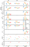Fig. 1. Best-fit transport parameters with their asymmetric uncertainties (from MINOS) and corresponding ${\chi }_{\text{min}}^2/\text{d}.\text{o}.\text{f}.$ and ${\chi }_{\text{nui}}^2/n_{\text{nui}}$ (next-to-last and last panels) for BIG, SLIM, and QUAINT (first, second, and third column). Different secondary species are colour-coded, with different symbols for ratios to C (crosses) and to O (circles): “Be/C NoLE2” stands for Be/C AMS-02 data without the two lowest rigidity points (orange triangles), and LiBeB/C (or /O) stands for the combined analysis of Li/C, Be/C, and B/C (or /O). See text for details.

A bit more puzzling is the large ${\chi }_{\text{min}}^2/\text{d}.\text{o}.\text{f}.$ difference (∼0.4) between Be/C and Be/O, which is significant in all models (orange crosses versus circles in the bottom panel of Fig. 1). The origin of this difference is attributed to the presence of an upturn in the low-rigidity Be/C data (orange symbols in the top panel of Fig. 2). As a consistency check, we fitted Be/C without the two lowest rigidity data points and find an excellent ${\chi }_{\text{min}}^2/\text{d}.\text{o}.\text{f}.$ (orange triangles, labelled “Be/C NoLE2” in Fig. 1). This procedure also brings the high-rigidity transport parameters in slightly better agreement (compare the orange crosses with their circle and triangle counterparts). Whether this is physically meaningful is difficult to say. With a better modelling of AMS-02 systematics, the situation could probably be clarified. If it remains, the presence of an upturn could hint at some subtle but important physics effect not considered yet.

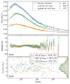Fig. 2. Flux ratios (top), residuals (centre), and $\stackrel{\sim }{z}$-scores (bottom) for B/C (blue circles), Be/C (orange squares), and Li/C (green triangles). The models (top panel) are calculated for BIG (solid line), QUAINT (dash-dotted line), and SLIM (dotted line), from the best-fit transport parameters of the combined analysis of all three species. The residuals and $\stackrel{\sim }{z}$-score are shown for SLIM only; the $\stackrel{\sim }{z}$-score is related to the usual z-score by a rotation in a base where the covariance matrix of data systematics is diagonal (see text for details).

We conclude that there is no significant difference using C or O (in the ratio), and in the following, we stick to the standard practice of using x/C ratios. However, in the combined analyses below, it should be kept in mind that whenever Be/C data are included, the ${\chi }_{\text{min}}^2/\text{d}.\text{o}.\text{f}.$ is slightly “degraded” compared to the results we would have obtained using Be/O. It should not straightforwardly be interpreted as a poorer quality of the model.

3.2. Separate vs combined analysis

The cross symbols in Fig. 1 show the best-fit transport parameters from the analysis of AMS-02 Li/C (green), Be/C (orange), and B/C (blue) separately. The parameters are compatible at the 1σ level for all models for Li/C and B/C. For Be/C, the agreement is also very good for SLIM, but with small deviations for BIG and QUAINT. The difference is not significant enough to conclude on a preference for SLIM.

As the data uncertainties have the same status (see Appendix B), we can perform a combined analysis of the three species (red symbols) without further complication. The combined fit leads to slightly tighter constraints on the transport parameters (red symbols in Fig. 1) except for BIG, probably because of degeneracies between its too many parameters. The ${\chi }_{\text{min}}^2/\text{d}.\text{o}.\text{f}.$ are acceptable⁶ (see also Table 1), though we observe a jump of ${\chi }_{\text{nui}}^2/n_{\text{nui}}$ from ∼0 (in single-species fits) to ∼1.5 (in the combined fit). This is attributed to cross-section nuisance parameters wandering away from their input values. The partial degeneracy between the diffusion coefficient normalisation K₀ and the production cross-section is lifted in the simultaneous fit: K₀ is enforced to be the same for all species, so that cross-section degrees of freedom are now used, adding a penalty in ${\chi }_{\text{nui}}^2/n_{\text{nui}}$. We come back to this very important issue in Sect. 5.

The resulting best-fit ratios are shown against the data in Fig. 2. The top and middle panels show the total uncertainties (statistical plus systematics in quadrature), and they overestimate the real uncertainties used in the χ² analysis. As introduced in Boudaud et al. (2020), a graphical representation of the “rotated” score (denoted $\stackrel{\sim }{z}$-score) provides an unbiased view accounting for the role of correlations in data systematics. The rotated base is defined such that the covariance matrix of uncertainties is diagonal,

$$\begin{array}{c}\hfill \stackrel{\sim }{\mathcal{C}}=U\mathcal{C}{U}^{\mathrm{T}},\end{array}$$(6)

with U an orthogonal rotation matrix. In this new base, we define the rotated residual

$$\begin{array}{c}\hfill {\stackrel{\sim }{z}}_i={\stackrel{\sim }{x}}_i/{\stackrel{\sim }{\sigma }}_i,\end{array}$$(7)

with the rotated difference and rotated diagonal systematics respectively defined to be

$$\begin{array}{c}\hfill {\stackrel{\sim }{x}}_i\equiv {\displaystyle \sum _j{U}_{\mathit{ij}}({\mathrm{model}}_j-{\mathrm{data}}_j)\mathrm{and}{\stackrel{\sim }{\sigma }}_i\equiv {\sqrt{\mathcal{C}}}_{\mathit{ii}}.}\end{array}$$(8)

In the rotated base, rigidities are replaced by pseudo (or rotated) rigidities, defined to be

$$\begin{array}{c}\hfill {\stackrel{\sim }{R}}_i={\displaystyle \sum _j{U}_{\mathit{ij}}^2{R}_j.}\end{array}$$(9)

Because the rotation is small, with U close to unity, the pseudo rigidity ${\stackrel{\sim }{R}}_i$, for the case of AMS-02 data, is not very different from the physical value R_i.

The $\stackrel{\sim }{z}$-score is shown in the bottom panel of Fig. 2 as a function of $\stackrel{\sim }{R}$ for Li/C, Be/C, and B/C. By construction

$$\begin{array}{c}\hfill {\chi }^2={\displaystyle \sum _i{\stackrel{\sim }{z}}_i^2,}\end{array}$$(10)

and we can also build a histogram of ${\stackrel{\sim }{z}}_i$ values, as shown on the right side of the panel. This should follow a centred Gaussian of width unity if the model matches the data. This is indeed mostly the case, except for Be/C (orange line) which has too large tails (we recall that the deviation is partly driven by the two Be/C low-energy data points). More quantitatively, the distance between the model and data from the global fit is ${\chi }_{\text{B/C}}^2=62.8$, ${\chi }_{\text{Li/C}}^2=78.5$, and ${\chi }_{\text{Be/C}}^2=95.7$ for 68 data points each.

3.3. Updated benchmark models and low-rigidity break

We list in Table 1 the best-fit transport parameters obtained from the combined analysis of LiBeB AMS-02 data. Compared to our previous analysis of B/C ratio only, several differences are worth noting.

Intermediate-rigidity parameters (K₀, δ). For SLIM, the combined analysis leads to a similar value of the diffusion slope, though with smaller uncertainties (δ = 0.51 ± 0.02). For the other two models with more free parameters (partially degenerated), the present analysis gives slightly higher values, so that all models now converge to the same δ value. In the combined analysis, the diffusion coefficient normalisation is K₁₀/L ≈ (0.024,  0.025,  0.027)±0.004 for (BIG, SLIM, QUAINT) to compare to K₁₀/L ≈ (0.030,  0.028,  0.033)±0.003 in the B/C-only analysis G19⁷. There is a significant trend towards lower values in all models (∼10%). This is another illustration that production cross-section degrees of freedom (nuisance parameters) are now used in the combined fit. Somehow, a smaller production cross-section was required for B, leading to a smaller value for K₀ (actually K₀/L). We discuss the meaning of the derived cross-section values in Sect. 5.

Low-rigidity parameters (V_c, V_a, η, δ_l, R_l). There is also a significant change with respect to the B/C-only analysis in this regime. A low-rigidity break is clearly identified at R_l ≈ 4.6 ± 0.3 with δ_l ≈ 0.63 ± 0.3 for both BIG and SLIM, whereas BIG was compatible with no break in the B/C-only analysis of G19. The diffusion coefficient in QUAINT only enables a modification in the sub-relativistic regime (β^η term in Eq. (1)) and with η ≈ −1.6 ± 0.5, a clear upturn is observed compared to the B/C-only analysis (compatible with η = 0). Concerning reacceleration, whereas BIG could find best-fit regions with large V_a (up to 80 km s⁻¹ in the B/C analysis), the combined analysis shrinks BIG towards SLIM (neither reacceleration nor convection); even in QUAINT the need for reacceleration is halved.

Low-rigidity break. Figure 3 shows 1σ contours of the diffusion coefficient⁸, providing a direct illustration of the low-rigidity break: the preference of a break or upturn is significant in all configurations. We investigate in Appendix D whether low-energy data (ACE-CRIS data; George et al. 2009) can provide similar but independent conclusions. They do not, but are nevertheless in broad agreement with models derived from the AMS-02 LiBeB constraints. The low-rigidity diffusion upturn is thus supported by three observations: (i) the combined analysis of various species points towards a break or upturn at GV rigidities; (ii) low-energy data are consistent with the presence of an upturn; (iii) although BIG has the largest number of free parameters, its parameter space prefers to shrink to that of the minimal configuration SLIM, which favours a low-rigidity break.

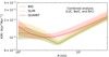Fig. 3. Best-fit and 1σ contours for K(R), see Eq. (1), reconstructed from the best-fit transport parameters (and their covariance matrix) from the combined LiBeB analysis. Three models are shown: BIG (orange), SLIM (green), and QUAINT (red). In the low-rigidity range, the factor β in Eq. (1) makes K(R) dependent on the CR species; shown are the result for A/Z = 2. See text for discussion.

3.4. Propagation uncertainties in benchmark models

From the previous analysis (combined fit of Li,/C, Be/C, and B/C AMS-02 data), we assess the propagation uncertainties on calculated secondary-to-primary ratios. From the best-fit transport (and nuisance parameters) and their correlations, we draw N realisations of the parameters, calculate the associated CR fluxes, and extract from their distribution the desired quantiles (in each rigidity bin) for any species.

We show in Fig. 4 the 68% contours (1σ) with respect to the median for various models (top panel), various parameters (middle panel), and various secondary-to-primary ratios (bottom panel). In the configuration with the fewest number of free parameters (SLIM), the model uncertainties are at the level of or even below the data uncertainties shown in Fig. A.1. At variance, the larger the number of parameters the more degenerate the configuration, so that QUAINT and BIG model uncertainties encompass the data uncertainties. Nevertheless, for all transport configuration, the rigidity at which the calculation is best constrained is at ∼10 GV, corresponding to the region where AMS-02 data uncertainties are at a minimum.

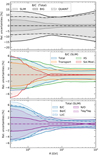Fig. 4. Propagation relative uncertainties (1σ contours with respect to median) as a function of rigidity based on the constraints set by the combined LiBeB analysis. Top panel: comparison of total transport uncertainties from BIG (solid), SLIM (dashed), and QUAINT (dash-dotted). Middle panel: separate uncertainty contributions from nuclear cross-sections (green), solar modulation (red), and transport (range) in SLIM. Bottom panel: comparison (in SLIM) of various calculated secondary-to-primary ratios within the combined LiBeB constraint.

The total model uncertainties account for model parameter correlations, and include transport, cross-sections, and solar modulation. The middle panel of Fig. 4 shows how each of these ingredients contributes to the error budget: below 1 GV, solar modulation uncertainties are dominant, then cross-section uncertainties are dominant from ∼1 to ∼10 GV, and transport and cross-section uncertainties are equally important above ∼10 GV. Because of correlations, the total uncertainties (blue contours) are smaller than the individual ones.

The bottom panel of Fig. 4 illustrates that, once the propagation parameters have been constrained by some specific secondary-to-primary ratios, all other similar ratios contribute the same level of modelling uncertainties⁹. This is not surprising as the baseline modelling uncertainty is from the transport parameters, which applies to all propagated species.

3.5. Discussion

It is interesting to compare our results to those of Evoli et al. (2019). These authors rely on a similar 1D propagation model, but discard reacceleration arguing that in general, it is incompatible with the models based on self-generated waves that they consider. They first take AMS-02 fluxes for B, C, N, and O in combinations differing from ours, from which they obtain δ = 0.63, V_c = 7 km s⁻¹, and K₀ = 1.1 × 10²⁸ cm² s⁻¹, the last corresponding to K₁₀/L = 0.039 kpc Myr⁻¹. This is compared with the typical values we find δ ∈ [0.45, 0.53] and K₁₀/L ∈ [0.020, 0.031] kpc Myr⁻¹ from our configurations (reacceleration or pure diffusion). Evoli et al. (2019) do not provide an estimate of the uncertainty, but our results seems difficult to reconcile with theirs¹⁰. The origin of the difference may occur because these authors do not account for a low-rigidity break and only fit the data above 10 GV. It may also be related to the fact that using more primary data than secondary ones in the fit biases the determination of the transport parameters (see comments above). Interestingly, although our diffusion slopes differ, we find in our models similar conclusions regarding the different source slopes needed for protons, helium, and heavier nuclei to reproduce the data of Boudaud et al. (2020), with an injection spectrum for helium (resp. protons) ∼0.03 harder (resp. ∼0.05 softer) than that of nuclei.

Another interesting comparison can be achieved with the results of Boschini et al. (2020), where the authors use the Galprop and HelMod codes (Boschini et al. 2019) to fit absolute fluxes of Li, Be, B, C, N, and O, as well as the B/C ratio. While their main focus is on the interstellar spectrum and on the hypotheses around the high-rigidity break, we can still compare their best fit for the intermediate rigidity parameters. They obtain δ = 0.415 ± 0.025 and K₁₀/L ≈ 0.047 ± 0.008 kpc Myr⁻¹, which is many sigma away from ours. This can be explained by the methodology used, which is quite different; mainly, they do not allow for low-rigidity breaks in the diffusion coefficient and do not treat the systematic uncertainties with covariance matrices as we do. Interestingly, the authors also report an overproduction of Be and a deficit of Li at high energies. Since we have chosen to use nuisance parameters to handle nuclear cross-section uncertainties, we do not experience the same difficulty, and show that mild variation (within the current uncertainties) of the normalisation can resolve this tension; specifically, Boschini et al. (2019) add primary Li to correct for a 20−25% deficit, while we increase the total Li production cross-sections by 13% (see Sect. 5).

4. Accommodating ³He/⁴He and N/O data

Two other AMS-02 ratios are possibly relevant to our study, namely the isotopic ratio ³He/⁴He (Aguilar et al. 2019) and the partly primary N/O ratio (Aguilar et al. 2018b). For reasons discussed below, these ratios have specificities that prevent them from being readily employed in a combined analysis. However, they still provide useful constraints complementary to the ones set by Li, Be, and B.

4.1. Motivations and complications

4.1.1. Fitting N/O

The N/O ratio evolves from a secondary N fraction of ∼70% at a few GV to ≲30% above 1 TV (Aguilar et al. 2018b). In principle, it is not ideal to study transport parameters as it is no longer independent from source parameters. However, it enables a test of the universality of transport for a heavier species and is worth considering.

As shown in G19, primary fluxes and in particular C and O AMS-02 data can be nicely reproduced in our model by fitting the transport parameters on B/C and then using a simple universal power-law source spectrum (not fitted). We checked that C and O AMS-02 data are also reproduced in our combined LiBeB analysis. The primary content of N is thus expected to be correctly predicted using the same source spectral index as that of C and O. With this caveat, fitting N/O is expected to bring complementary constraints on the transport parameters, all the more because their broken-down data uncertainties are similar to those of Li/C, Be/C, and B/C (see Appendix A). In all analyses involving N/O data below, an extra nuisance parameter for the production cross-section of N is added (see Table B.1).

4.1.2. Fitting ³He and ⁴He

Waiting for AMS-02 deuterium data, the pure secondary ³He is the best option to test the universality of transport towards lighter nuclei. In addition, the ³He/⁴He ratio was shown to provide complementary and competitive constraints compared to those obtained from B/C (Coste et al. 2012; Tomassetti 2012b; Wu & Chen 2019). However, with the high precision of AMS-02 data (Aguilar et al. 2019) on an unprecedented energy range, directly fitting ³He/⁴He is no longer recommended. As explained below, unbiased conclusions can only be reached by fitting simultaneously ³He and ⁴He.

All production cross-sections are assumed to follow the straight-ahead approximation in which the fragment carries out the same kinetic energy per nucleon as the parent. On the other hand, both solar modulation and diffusion have a similar impact on species with the same R. With $R\approx (A/Z)\sqrt{E_{k/n}(E_{k/n}+2m_p)}$, species with similar A/Z at a given E_k/n also have similar R (and vice versa). As a result, ratios of such secondary-to-primary species are independent of the source spectra when taken per E_k/n or R, and all feel the same transport at a given E_k/n or R; an example is B/C, with both the dominant ¹⁰B and ¹²C contributions having A/Z = 2. This is no longer the case for ³He/⁴He, having respectively A/Z = 1.5 and 2, so that neither the fit versus E_k/n nor R is appropriate. Hence, contrary to the analysis of LiBeB, we cannot directly fit ³He/⁴He and are forced to fit both ³He and ⁴He simultaneously.

To ensure that ⁴He data are reproduced correctly, we allow for a flexible enough parametric formula for the ⁴He source term. These extra parameters are added in the combined fit; in practice, the best-fit source spectrum is close to a pure power law. Given that the number of data points is small and that they spread over a limited energy range (22 and 25 data for ³He and ⁴He from 3 to 20 GV), the determination of the transport parameters is expected to remain driven by the LiBeB combined data (205 data points from 3 GV to 2 TV). With these provisos, the fit on ³He provides a complementary constraint on the transport parameters. To account for uncertainties in the production cross-section of ³He, an extra nuisance parameter is added in the fit (see Table B.1) whenever ³He data are considered.

Owing to the experimental challenges of separating these isotopes, the two high-precision datasets at hand are those of AMS-02 (Aguilar et al. 2019) and PAMELA (Adriani et al. 2013, 2016). The BESS-Polar II data are not considered here, because only preliminary analyses are available (Picot-Clémente et al. 2015a, 2017). For the sake of consistency, only AMS-02 data are fit, but PAMELA data are used for post-fit visual inspection. The choice remains as whether to fit AMS-02 data as a function of kinetic energy per nucleon or rigidity, both being provided in Aguilar et al. (2019). We argued in Derome et al. (2019) that opting for one or the other brought different systematic uncertainties in the B/C case (because of the unknown isotopic content of the elements biasing the conversion). However, here the conversion to go from different energy types is exact for ³He and ⁴He. In the AMS-02 analysis (Aguilar et al. 2019), ³He and ⁴He fluxes and systematics are provided as a function of kinetic energy per nucleon, from three separate sub-detectors. A covariance matrix of uncertainties can be built either in E_k/n or R (see Appendix A.2), so that any of them can be used with the same end result.

4.2. Transport parameters from LiBeB, N/O, ³He, and ⁴He

Figure 5 shows the best-fit parameters from the simultaneous analysis of AMS-02 Li/C, B/C, Be/C (red crosses), further combined with N/O (turquoise squares) or ³He and ⁴He (violet circles), or with both (brown triangles).

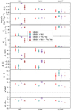Fig. 5. Best-fit transport parameters and uncertainties with the corresponding ${\chi }_{\text{min}}^2/\text{d}.\text{o}.\text{f}.$ and specific contribution from nuisance parameters (next-to-last and last columns) for different combinations of AMS-02 data: combined fit of LiBeB (red crosses); LiBeB and N/O combined (turquoise squares); LiBeB and 3He/4He combined (purple circles); LiBeB, 3He/4He, and N/O combined (brown triangles). From left to right: models BIG, SLIM, and QUAINT.

For all configurations (BIG, SLIM, and QUAINT), adding N/O in the fit (turquoise squares) improves the ${\chi }_{\text{min}}^2/\text{d}.\text{o}.\text{f}.$ and ${\chi }_{\text{nui}}^2/n_{\text{nui}}$ values and better constrains the transport parameters. This indicates that N/O data were already consistent with the results of the LiBeB combined fit. The situation is less clear-cut when adding ³He and ⁴He. Whereas the data are easily accommodated for by the model for QUAINT (same ${\chi }_{\text{min}}^2/\text{d}.\text{o}.\text{f}.$ and parameter values), the fit is not so good for SLIM, with an increased ${\chi }_{\text{min}}^2/\text{d}.\text{o}.\text{f}.$ and ${\chi }_{\text{nui}}^2/n_{\text{nui}}$ and a δ_l marginally compatible with the LiBeB analysis. Even more significant is the behaviour of BIG: whereas in the case of the LiBeB combined analysis BIG’s parameter space shrank towards SLIM, the small amount of ³He data (compared to LiBeB) completely shifts BIG’s parameter space towards QUAINT (with reacceleration and also convection). This behaviour remains the same for the LiBeB, N/O, ³He, and ⁴He combined fit (brown triangles). This demonstrates the strong sensitivity of ³He to the low-rigidity transport parameters.

Figure 6 shows a comparison between the models and data (top panels) and the corresponding residual and $\stackrel{\sim }{z}$-score (QUAINT only, bottom panels) for the combined fit of AMS-02 Li/C, Be/C, B/C, N/O, ³He, and ⁴He data. The above conclusions and goodness of fit to the data are illustrated in the various panels. All models fit equally well the N/O data (top panel) and ⁴He data (second panel). For the latter, the very good fit ${\chi }_{{}^{\text{4}}\text{He}}^2/n_{\text{data}}=(22.7,23.8,18.9)/25$ for (BIG, SLIM, QUAINT) validates the procedure depicted in the previous section, i.e. it ensures that the fit of ³He is based on the correct spectrum of its main progenitor. We obtain ${\chi }_{{}^{\text{3}}\text{He}}^2/n_{\text{data}}=(25.5,41.4,21.9)/22$ for (BIG, SLIM, QUAINT). All models (second panel) slightly overshoot the data at a few GV, with QUAINT giving a very good fit, followed by BIG, but with SLIM giving a poor fit.

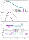Fig. 6. Model calculation and data (first and second panel), residuals (third panel), and $\stackrel{\sim }{z}$-score (fourth panel) for N/O (turquoise circles), 4He (red squares), and 3He (pink triangles). For readability, He isotopic fluxes are multiplied by R2.2. Two top panels: model calculations for BIG, SLIM, and QUAINT along with their respective post-fit modulation level, two bottom panels: restricted to the best-fit configuration QUAINT. The inset shows the distance between the model and specific datasets, calculated from ${\chi }^2=\sum _i\stackrel{\sim }{z_i}$. All models are calculated from the best-fit parameters of the combined analysis of Li/C, Be/C, B/C, N/O, 3He, and 4He.

4.3. Impact of data correlation length

The goodness of fit of He isotopic data highlighted in the previous section must be taken with a grain a salt. The quantitative agreement between the model and the data depends on the correlation length taken for ³He and ⁴He data, as illustrated in Fig. 7. The figure shows that the acceptance systematic uncertainties, which dominates the uncertainty budget (see Fig. A.3) and whose correlation length value is not strongly determined, strongly impact the conclusions.

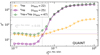Fig. 7. Distance (post-fit χ2) between data and models varying the correlation length ${\mathcal{l}}_{\rho }^{\text{Acc Rec}\&\text{Sel}}$ (in decades) of 3He and 4He data for QUAINT. The horizontal dotted line highlights the number of data points, indicating roughly the position at which χ2/d.o.f. ≈ 1.

The calculation in the previous section and in Fig. 6 corresponds to ${\mathcal{l}}_{\rho }^{\text{Acc Rec}\&\text{Sel}}\text{=0}.\text{05}$. From Fig. 7 we conclude that if we had chosen a shorter (resp. longer) correlation length, we would have concluded that prediction for the He isotopes were in perfect agreement (resp. in tension) with the data; however, this would mostly leave unchanged the values of the best-fit transport parameters. This situation is very similar to that of the B/C case, studied in detail in Derome et al. (2019), for which ${\mathcal{l}}_{\rho }^{\text{Acc}.\text{res}.}$ was set to 0.1, a value also used for LiBeB and N/O data in this analysis (see Appendix A.1).

4.4. Discussion

We can briefly compare our results to the work of Wu & Chen (2019), which is the only analysis using recent ³He/⁴He data. These authors analyse PAMELA data with the Galprop code, which relies on the same production cross-sections we use here, i.e. from Coste et al. (2012)¹¹. They obtain a good fit to ²H/⁴He, ³He/⁴He, H, and He data, but then their model undershoot $\overline{p}$ and B/C data by many σ. Although our fit is not perfect, we clearly do not face the same issues. Several reasons could explain this difference, like the use of cross-section nuisance parameters and covariance matrices of uncertainties. Another likely reason could be that fitting high-precision primary species (e.g., H and He)–whose fluxes depend on both the source and transport parameters, and with fewer and less precise data for the secondary species (²H/⁴He, ³He/⁴He, or even $\overline{p}$)–may bias the transport parameter determination (Coste et al. 2012). The same issue might be present in several recent studies, for instance, Jóhannesson et al. (2016), Korsmeier & Cuoco (2016), Wu & Chen (2019), and Evoli et al. (2019). It could and should be fully assessed with the help of simulated data in future analyses.

5. Nuisance parameters post-fit values

In the previous section, we found (with some caveats) that all the data could be reproduced by all of our model configurations. For this conclusion to hold, however, we must check that nuisance parameters behave as expected. Given that the number of data points (∼300) is much larger than the number of nuisance parameters (∼10), the latter degrees of freedom could be used at a cheap cost to improve the fit. If so, this would lead to conflicts with the priors and uncertainties expected on these parameters, disfavouring the associated model configuration (BIG, SLIM, or QUAINT). We check below that this is not the case, or only mildly.

5.1. Consistency of solar modulation values

As described in Sect. 2.3.4, AMS-02 data in the analyses are set to ϕ_prior = 676 ± 100 MV. Post-fit values of the AMS-02 modulation level were only shown in the plots of the previous section, and we now comment on them.

If we come back to the combined analysis of the LiBeB ratios, the legend of Fig. 2 shows that the post-fit AMS-02 modulation level for all configurations is within 30 MV of the values taken for the prior. Including low-energy data in the fit (Appendix D) also leads to consistent post-fit modulation levels for all datasets. For the combined fit with all species, the post-fit values are read off from Fig. 8, which provides a further illustration of the He isotopes goodness of fit. The modulation levels in the legend correspond to post-fit values of AMS-02 data. Whereas BIG leads to closest value to the prior, SLIM and QUAINT are respectively 1σ below and above it, starting to be close to their allowed uncertainties.

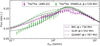Fig. 8. 3He/4He as a function of Ek/n for AMS-02 (purple squares) and PAMELA (green crosses)–the latter combine data from two different analysis, respectively PAMELA-ToF and PAMELA-Calorimeter (Adriani et al. 2016). All models are calculated from the best-fit parameters of the combined analysis of Li/C, Be/C, B/C, N/O, 3He, and 4He AMS-02 data. Different line styles show different model configurations (BIG, SLIM, and QUAINT) and their respective post-fit solar modulation level in purple. Green lines show the same model calculations but modulated at the PAMELA expected value of 539 MV.

It is also instructive to compare the model predictions with the PAMELA data (Adriani et al. 2016). For these data the modulation is estimated to be 539 MV at which the model calculations are taken (green lines): the best model in that case is SLIM, because AMS-02 and the PAMELA data are then expected to be equally modulated, though this is not very realistic. On the other hand, BIG and QUAINT both overshoot by ∼2σ the PAMELA data points. In the context of a very challenging experimental measurement, it is difficult to conclude on the relevance of this difference. It could also be related to solar modulation features as we need to modulate two isotopes with different A/Z values.

At this stage, we conclude that post-fit values obtained for the modulation level of AMS-02 data are within the expected uncertainties. As highlighted by the comparison to the PAMELA data, further data taken at different periods in the modulation cycles could be very useful to conclude on the best transport configuration and on the consistency of solar modulation levels.

5.2. Consistency of nuclear cross-sections

We recall that for each selected reaction (inelastic or production), the NSS scheme enables several nuisance parameters (see Appendix B). The most important one is a normalisation, 𝒩_X, involved in the calculation of the CR quantity X. All these nuisance parameters have a prior 𝒩_prior ≈ 1 with a width σ ≈ 5% and σ ≈ 10% for inelastic and production cross-sections, respectively.

We look below into the correlation between this parameter and the normalisation of the diffusion coefficient, for several quantities and fit configurations.

5.2.1. Inelastic cross-section normalisation

The left panels of Fig. 9 show correlations for inelastic cross-sections in the plan XS norm-log₁₀(K₀) for SLIM (top) and QUAINT (bottom). The ellipses are calculated from the correlation matrix of best-fit parameters returned by HESSE; their widths are constructed from a trade-off between values found by HESSE and MINOS. All ellipses give the directions towards which log₁₀(K₀) would move if the cross-section normalisation were to change (and vice versa).

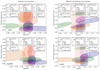Fig. 9. Correlations between the normalisation of the inelastic (left panels) or production (right panels) cross-sections and log10(K0), for models SLIM (top panels) and QUAINT (bottom panels). The various colours correspond to the normalisations of cross-sections involved in different CR species: Li (green), Be (orange), B (blue), N (turquoise), and 3He (crimson). The various symbols and line styles correspond to the post-fit values and ellipses (for the previously listed species) from various fit configurations: separate Li/C, Be/C, and B/C fits (“×” symbols and solid lines), combined Li/C, Be/C, and B/C fit (LiBeB for short, “+” symbols and dotted lines), combined LiBeB+N/O+3He+4He fit (“⋆” symbols and dashed lines). The horizontal grey dashed lines highlights the case of using unmodified cross-section datasets (T99 for inelastic and G17 for production, see Appendix B), i.e. ${\mathcal{N}}_{\mathrm{CR}}^{\mathrm{reac}.}=1$: the subscript in 𝒩 indicates the CR species associated with this nuisance parameter; the superscript shows the reaction used as a proxy for this CR. For production cross-sections (right panels), the normalisation parameters are not directly the value of the nuisance parameter, but are effective parameters, see Eq. (11). See text for discussion.

We first focus on the solid lines, corresponding to the cross-section normalisation parameters involved for the calculation of Li/C (𝒩_Li in green), Be/C (𝒩_Be in orange), or B/C (𝒩_B in blue). When these ratios are fitted separately, different best-fit log₁₀(K₀) values are obtained. The combined Li/C, Be/C, and B/C analysis forces log₁₀(K₀) to move towards the same value. As expected, the new ellipses (dotted lines) and best-fit values (cross symbols) moved from the old ones (plus symbols) mostly along the strongest correlation directions (ellipse principal axis). The normalisation nuisance parameters 𝒩_Li and 𝒩_B are within ±5% of the initial cross-section values (i.e. 1), but 𝒩_Be ≈ 1.15; the same behaviour is observed for both SLIM and QUAINT. This slightly larger value is possibly related to the possible statistical fluctuation on the AMS-02 low-energy data points discussed in Sect. 3.1. The combined analysis with LiBeB, N/O, and He isotopes leads to similar conclusions (compare dash-dotted and dotted line ellipses).

We recall that these normalisations are actually proxies for a much larger list of reactions (see Appendix B). We also recall that inelastic reactions overall impact the calculation at the level of a few percent and at low rigidity only (see left panels of Fig. B.1). We can furthermore state that these “effective” nuisance parameters are well-behaved and that their posterior values are within the expected uncertainties.

5.2.2. Production cross-section normalisation

We now turn to the case with higher impact, production cross-sections, in which model calculations for Li/C and Be/B, for example, can change by ∼10% over the whole rigidity range depending on the selected nuclear datasets (see right panels of Fig. B.1).

In Fig. 9 the right panels show correlation plots between the post-fit normalisation of the overall production of various species (Li, Be, B, N, and ³He) and the normalisation of the diffusion coefficient log₁₀(K₀). To account for the fact that the specific reactions (used as nuisance parameters) are merely proxies and only represent a fraction x of the total production of a CR species under scrutiny, we rescale our normalisation nuisance parameters ${\mathcal{N}}_{\mathrm{CR}}^{\mathrm{single}\mathrm{reac}\equiv \mathrm{proxy}}$, to obtain¹²

$$\begin{array}{c}\hfill {\mathcal{N}}_{\mathrm{CR}}^{\mathrm{eff}}=(1-x)+x{\mathcal{N}}_{\mathrm{CR}}^{\mathrm{proxy}}=1+x({\mathcal{N}}_{\mathrm{CR}}^{\mathrm{proxy}}-1).\end{array}$$(11)

The quantity shown in the y-axis of the plot can be directly taken as the global uncertainty on the total production of the species considered. The solid and dashed lines show the ellipses from separate and combined fits of Li/C, Be/C, and B/C. In the combined fits (cross symbols and dotted ellipses), the normalisations again move in the direction of the correlation to reach the best log₁₀(K₀). If N/O and He isotopes are added to the combined fit (star symbols and dashed ellipses), a further but minor displacement occurs. Similar behaviours are observed for both SLIM (top) and QUAINT (bottom).

From the position of the ellipses in the bottom panel of Fig. 9, we can refine the statement made in the previous section: the model is able to accommodate for all data, although it requires some small but significant modification of the production cross-sections with respect to the initial cross-section taken. The overall production must be a few percent different for B and ³He, ∼5% for Be and N, but ∼12% for Li. As illustrated in the Supplemental Material of Génolini et al. (2018), a 10% to 15% cross-section difference is easy to obtain for many individual channels. This translate into a similar (or smaller) “effective” uncertainty for the overall production if all cross-section reactions are weakly correlated (or uncorrelated, see Génolini et al. 2018).

From this analysis, we conclude that all production cross-sections end up within their expected values, even Li, which reaches the limit of its allowed uncertainties. However, the nuclear data for Li are scarce. For illustrative purposes, we show in Fig. 10 a comparison between the data (symbols) and the benchmark G17 parametrisations (Moskalenko et al. 2001; Moskalenko & Mashnik 2003) used in our analysis, for the most important production cross-sections contributing to Li and Be fluxes (Génolini et al. 2018). The required normalisation variation of a few percent for Be and ∼15% for Li are completely allowed by the present data quality. This whole discussion illustrates that at the level of precision of AMS-02 data, production cross-sections matter a lot in the context of combined analyses. Better nuclear data are mandatory to better assess the goodness of fit, and possibly reveal tensions between CR flux calculations and data for different species.

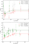Fig. 10. Data (symbols) and model (lines) comparison for the most important production cross-sections leading to Li (top panel) and Be (bottom panel) fluxes. Their respective contribution to the total flux production is reminded in brackets. The data are taken from Génolini et al. (2018) and the model is the GALPROP parametrisation (Moskalenko et al. 2001; Moskalenko & Mashnik 2003). See text for discussion.

6. Conclusions

We have shown that a propagation model is able to successfully reproduce all secondary-to-primary ratios recently published by the AMS-02 collaboration, i.e. Li/C, Be/C, B/C (Aguilar et al. 2018a), N/O (Aguilar et al. 2018b), and He isotopes (Aguilar et al. 2019). These model configurations are based on recent benchmark transport scenarios introduced in G19 and are updated here. In the context of a high-rigidity break at ∼200 GV, they confirm a diffusion slope in the intermediate regime of δ in the range [0.45, 0.53].

The combined analysis of different AMS-02 ratios (Li/C, Be/C, and B/C) or the separate analysis of these ratios combining AMS-02 and lower-energy data (ACE-CRIS) show an equal preference either for a low-rigidity break in the diffusion coefficient (at ∼4.6 GV with a slope change of ∼0.7) or an upturn below a few GV. This effective change in the diffusion behaviour could reveal a decrease in the CR pressure as CRs reach the non-relativistic regime (β dependence), or be related to some dissipation of the turbulence power spectrum (rigidity dependence). As in G19 where only B/C data where considered, two disjointed regions of the transport parameter space provide viable solutions to match the LiBeB data: a purely diffusive regime with a low-rigidity break (configuration dubbed SLIM), or a convection–reacceleration solution with either a diffusion break or an upturn of the diffusion slope at the non-relativistic transition (configurations labelled BIG and QUAINT); based on the data analysed so far, there is no strong quantitative argument for choosing one or the other. These two configurations are also able to reproduce N/O data and ³He and ⁴He fluxes. However, we find that ³He data are extremely sensitive to reacceleration, and considering them or not in the combined analysis moves the best-fit parameters between the two preferred regions of the parameter space. At variance with the B/C analysis only, the BIG configuration requires both reacceleration (∼50 km s⁻¹) and convection (∼10 km s⁻¹) in the combined analysis of all species. It is possible that the parametrisation of the low-energy cross-sections is too simple, and the diffusion coefficient at non-relativistic rigidities can also be much more complicated (e.g., Schlickeiser et al. 1991).

Combining other secondary species, when released by the AMS-02 collaboration (e.g., ²H, F, Na...up to sub-Fe), or understanding the low-energy interstellar Voyager data (Cummings et al. 2016) should help decipher the low-energy transport of CRs.

Compared to other similar efforts in the literature (Jóhannesson et al. 2016; Cummings et al. 2016; Korsmeier & Cuoco 2016; Wu & Chen 2019; Evoli et al. 2019; Boschini et al. 2020), the decisive factor in our approach is to account for nuisance parameters for nuclear cross-sections and for rigidity correlations in the systematics of AMS-02 data; as in previous studies, we also use nuisance parameters for solar modulation levels. Firstly, as already demonstrated on B/C in Derome et al. (2019), the value of the correlation length in specific data systematics is crucial not to bias the determination of the transport parameters. These correlations are difficult to evaluate and are not provided in the AMS publications; however, these publications contain sufficient information to build them from educated guesses. We further show here that these correlations strongly impact the quantitative estimate of the goodness of fit to the data, especially for ³He, hence hampering our ability to draw statistically sound conclusions on the universality of our effective model for light species. Secondly, nuisance parameters provide extra degrees of freedom that allow us to directly propagate various uncertainties in the sought transport parameters. For instance, we find that below a few GV, solar modulation and production cross-sections are the dominant sources of uncertainties; above a few GV, transport and production cross-sections are the dominant ones. In any analysis, post-fit values of the nuisance parameters should not wander too far away from their allowed ranges, and we checked that they are all within their 1σ values in our analyses. These values are especially important and interesting for the case of production cross-sections. Whereas in the case of a single secondary-to-primary fit, the production cross-section normalisation is partly degenerate with K₀ (normalisation of the diffusion coefficient), this degeneracy is lifted in combined secondary-to-primary ratio analyses (because the same K₀ value is enforced). Inspecting the post-fit values for the production cross-sections, we find deviations going from a few percent (for ³He, Be, B, and N) up to 15% for Li with respect to the nuclear model values. This is in the ballpark of the estimated uncertainties for the production of these species, but it strengthens the need for better nuclear data in order to fully benefit from AMS-02 data precision; better nuclear data are also needed to draw stronger conclusions on the consistency of transport for all CR species.

Acknowledgments

We thank our CR colleagues at Annecy and Montpellier, and in particular J. Lavalle, A. Marcowith, P. Salati, P. Serpico for their very helpful feedback and discussions. We also thank A. Oliva for very useful comments. This work has been supported by the “Investissements d’avenir, Labex ENIGMASS”, by the French ANR, Project DMAstro-LHC, ANR-12-BS05-0006, and by Villum Fonden under project no. 18994.

References

Appendix A: Covariance matrices of systematic errors

The correlation between the AMS-02 data points can be taken into account by using covariance matrices for the fit. However, these matrices are not available and must be estimated from the information found in the AMS-02 publications. Following Derome et al. (2019), the relative covariance ${(C_{\text{rel}}^{\alpha })}_{ij}$ between rigidity bin R_i and R_j is taken to be

$$\begin{array}{c}\hfill {(C_{\mathrm{rel}}^{\alpha })}_{\mathit{ij}}={\sigma }_i^{\alpha }{\sigma }_j^{\alpha }exp(-\frac{1}{2}\frac{(log{(R_i/R_j)}^2}{{({\ell }_{\rho }^{\alpha })}^2}),\end{array}$$(A.1)

with ${\sigma }_i^{\alpha }$ the relative uncertainty of error type α at bin i and ${\mathcal{l}}_{\rho }^{\alpha }$ the correlation lengths for error type α (in unit of rigidity decade). The correlation length ℓ_ρ of each systematic was carefully chosen to best reflect the physics process behind the associated systematics (Derome et al. 2019). From the correlation length we can also form correlation matrices

$$\begin{array}{c}\hfill c_{\mathit{ij}}^{\alpha }=\frac{{\mathcal{C}}_{\mathit{ij}}^{\alpha }}{\sqrt{{\mathcal{C}}_{\mathit{ii}}^{\alpha }\times {\mathcal{C}}_{\mathit{jj}}^{\alpha }}}·\end{array}$$(A.2)

A.1. Li/C, Be/C, B/C (or ratios with O), and N/O

Figure A.1 shows statistical (Stat.) and systematic uncertainties provided by the AMS-02 collaboration (Aguilar et al. 2018a), i.e. acceptance (Acc.), scale (Scale), and unfolding (Unf.); the three line thicknesses (from thin to thick) and shades (from dark to light) correspond to N/O, B/C, Be/C, and Li/C ratios. As motivated and detailed in Derome et al. (2019), “Acc.” is further broken down in three more systematics, “Acc. norm.”, “Acc. LE”, and “Acc. res.”.

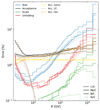Fig. A.1. Comparison of statistical and systematic uncertainties for N/O, B/C, Be/C, and Li/C (from thin to thick shaded lines). Values are taken from Aguilar et al. (2018a,b), except for “Acc. norm.”, “Acc. LE”, and “Acc. res.”, which are broken-down from Acc. uncertainties. See text for details.

For all species we observe that (i) at high rigidity, statistical uncertainties are dominant, especially for Be (medium-thick solid blue line), the less abundant of all the secondary species, see Fig. 2; (ii) at intermediate rigidities, “Acc. res.”, the most difficult systematics to derive a correlation length for (see below), is dominant; (iii) at low-rigidity, “Acc. LE”, which has a short correlation length (see below), is dominant, especially for B/C (thin-dashed black line). Despite some small differences in uncertainties between the species, we can conclude they all have the same status in the context of fits and conclusions that can be drawn from their fits (see Sect. 3).

The correlation matrices $c_{\mathit{ij}}^{\alpha }$ are shown in Fig. A.2. They are taken to be the same for the three secondary-to-primary ratios Li/C, Be/C, and B/C (and also ratios to O). These neighbour species have similar interactions in the detector, hence the same correlation lengths for their systematics. As illustrated in the various panels, statistical uncertainties (“Stat.”, ℓ_ρ = 0) are fully uncorrelated by definition, whereas the scale systematics (“Scale”, ℓ_ρ = ∞), is taken to be an overall normalisation. The “Acc.” systematics has several components, going from a quite correlated (“Acc. norm.”, ℓ_ρ = 1 decade) to less correlated (“Acc. res.”, ℓ_ρ = 0.1 decade) component. The overall covariance matrix for “Acc.” (top right panel) is a non-trivial combination of the correlation matrices (three bottom right panels) and relative uncertainties shown in Fig. A.1: it is dominated by “Acc. LE” at low rigidity and by “Acc. res.” above, with large wings from “Acc. norm.”. The correlation length of all combined uncertainties (top left panel) reflects the dominance of statistical uncertainties at high rigidities, and is again a non-trivial combination of all shown systematics. We recall that the exact choice of the correlation lengths for most systematics is not critical when fitting the data, except for “Acc. res.” (Derome et al. 2019): consistency arguments from the B/C analysis provided a preferred range, and for definiteness ${\mathcal{l}}_{\rho }^{\text{Acc}.\text{res}.}=0.1$ was chosen in order to have ${\chi }_{\text{min}}^2/\text{d}.\text{o}.\text{f}.\approx 1$ in the B/C analysis.

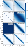Fig. A.2. Correlation matrices colour-coded from zero (no correlation, white) to one (full correlations, blue). Three bottom panels: systematics whose amplitude are shown in Fig. A.1. Top right panel: correlation matrix from all acceptance uncertainties, top left panel: that from all uncertainties combined.

A.2. ³He and ⁴He

The various contributions to the AMS-02 ³He and ⁴He systematics are broadly described in Aguilar et al. (2019). They originate from:

• the rigidity and β resolution function, “Resol.”;

• the trigger efficiency, “Trigger”;

• the geomagnetic cutoff, “Geo. cutoff”;

• reconstruction and selection efficiencies for acceptance, “Acc. Rec.& Sel.”;

• inelastic cross-sections for acceptance, “Acc. norm”;

• background contamination, “Background”.

We note that the break-down by the AMS-02 collaboration of systematics in various categories is different for He isotopes and Li, Be, B, and N elements. This is related to the different analyses required for elemental or isotopic flux reconstructions. Nevertheless, some similarities exist. In particular, “Geo. cutoff” and “Acc. Rec.& Sel.” for the He isotopes correspond to “Acc. LE” and “Acc. res” for the LiBeBN elements.

For each systematics we interpret the contributions at different rigidity values as a piece-wise power-law function. These functions are then rescaled at each rigidity bin so that the sum of all systematic errors matches the total systematic errors provided in Aguilar et al. (2019). This leads to our model for the AMS-02 ³He and ⁴He systematics, shown in the top panel of Fig. A.3.

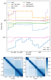Fig. A.3. Top panel: comparison of statistical and systematic uncertainties for 3He (thin lines) and 4He (thick lines) AMS-02 data. Bottom panel: correlation matrix for 3He (left) and 4He (right) as a function of R. All quantities are reconstructed from Aguilar et al. (2019); see text for details.

The covariance matrix associated with these systematics is then built from Eq. (A.1) based on an educated guess for their correlation length, ℓ_ρ (in unit of energy decade). In addition, as the fluxes are reconstructed using different detectors for the β measurements (TOF, RICH-NaF, RICH-AGL) with different selections and acceptances, we can assume that some contributions in the systematic are uncorrelated between the different associated rigidity regions. Here we assume that only the “Resol.” contribution corresponds to this case. For Resol., all covariance matrix elements corresponding to two different regions are set to 0 and the covariance matrix is then a block diagonal matrix.

For the correlation lengths, we take the following:

• ${\mathcal{l}}_{\rho }^{\text{Resol}.}=0.3$ as uncertainties from rigidity response function affect intermediate scales;

• ${\mathcal{l}}_{\rho }^{\text{Trigger}}=1.0$ because the uncertainty on the detector response affecting the trigger efficiency should produce a systematics strongly correlated for different rigidities;

• ${\mathcal{l}}_{\rho }^{\text{Geo}. \text{cutoff}}=0.3$; this contribution is similar to ${\mathcal{l}}_{\rho }^{\text{Acc}. \text{LE}}$ for the Li, Be, B, and N elements (same correlation length assumed);

• ${\mathcal{l}}_{\rho }^{\text{Acc}. \text{norm}}={\mathcal{l}}_{\rho }^{\text{Background}}=1.0$ since the uncertainty on cross-sections is mainly on their normalisations and then produce a strongly correlated systematic;

• ${\mathcal{l}}_{\rho }^{\text{Acc.Rec.}\&\text{Sel}}\text{=0}.\text{05}$, but similarly to ${\mathcal{l}}_{\rho }^{\text{Acc}. \text{res}}$ for elements, this number cannot be easily defined. As for ${\mathcal{l}}_{\rho }^{\text{Acc}. \text{res}}$, this systematics dominates the total error budget of the flux. The dependence of ${\chi }_{\text{min}}^2/\text{d}.\text{o}.\text{f}.$ with this correlation length was discussed in Derome et al. (2019) for the B/C case, and it is discussed here in Sect. 4.3 for ³He- and ⁴He-related fits.

The bottom panel of Fig. A.3 shows the total correlation matrix for ³He and ⁴He. The contributions of the block diagonal matrices from the “Resol.” systematics are visible.

Appendix B: Nuisance parameters for Li, Be, B cross-sections

Following Derome et al. (2019), the uncertainties in the inelastic and production cross-sections for CR analyses are dealt with nuisance parameters in the χ². As shown and validated on the mock data, the presence of cross-section nuisance parameters ensures a minimally biased determination of the transport parameter. It also naturally propagates cross-section uncertainties to all derived propagation parameters (Derome et al. 2019). This approach was successfully used in G19 for the B/C analysis, and it is repeated here for all our minimisation studies; other approaches have been used in the literature to assess and propagate the cross-section uncertainties to CR fluxes (Tomassetti 2017; Reinert & Winkler 2018; Evoli et al. 2019).

Impact of cross-section uncertainties. The calculation of any CR quantity involves a large network of nuclear reactions, and it is not possible in practice to include uncertainties for all the reactions. Instead, we focus on the ones with the most impact, and use them as a proxy to capture the overall effect of the whole network (Derome et al. 2019). Lists of reactions ranked by decreasing contribution for the production of Li, Be, B, and N can be found in Génolini et al. (2018). For illustration, we show in Fig. B.1 a selection of these reactions in the context of the calculation of the Li/C (first and third column) and Be/C (second and fourth column) ratios¹³; the two leftmost panels are related to inelastic cross-sections, the two rightmost to production cross-sections. The blue curves, associated with the right y-axis ticks and labels, illustrate the relative differences between several cross-section parametrisations available (from ∼10% to ∼25%). The black curves, associated with the left y-axis ticks and labels, show the impact of these differences on the calculated secondary-to-primary ratio: the ∼10% difference between inelastic cross-sections translates into a ∼1 − 2% difference only on Li/C and Be/C, whereas the ∼25% differences between production cross-sections translate in ∼5 − 10% differences on the CR ratios; see Derome et al. (2019) for the origin of these differences. The bottom row shows the impact of changing all cross-sections of the network at once (and not just one at a time): the full variation is typically captured by the combination of the few above-selected cross-sections, validating the choice of using the latter as proxies for the whole network.

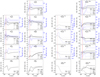Fig. B.1. Impact of inelastic (left) and production (right) cross-section uncertainties on Li/C (first and third column) and Be/C (second and fourth column) ratio for specific reactions as a function of rigidity. In each panel the relative difference between (inelastic or production) cross-section parametrisations with respect to a reference one is shown in blue (associated with the right y-axis), whereas the impact on the calculated ratio (in model SLIM) of varying the cross-section is shown in black (associated with the left y-axis). To guide the eye, the vertical red line indicates the rigidity of the first AMS-02 data point. The bottom panels show the overall impact when all reactions (i.e. all nuclei in the network) are replaced. Inelastic cross-sections are B94 (Barashenkov & Polanski 1994), W96 (Wellisch & Axen 1996), T99 (Tripathi et al. 1996, 1999), and W03 (Webber et al. 2003). Production cross-sections are W98 (Webber et al. 1998a,b,c), S01 (Soutoul, priv. comm.), W03 (Webber et al. 2003), and G17 (Moskalenko et al. 2001; Moskalenko & Mashnik 2003).

Normalisation, Scale, and Slope (NSS) and nuisance parameters. To properly propagate cross-section uncertainties on the calculated secondary-to-primary ratios, the trick is to find some parametrisations or transformation laws that allow us to encompass the sets of possible cross-section values. As noted in Derome et al. (2019), this is not a trivial task given the variety of production cross-section shapes. The transformation laws used here are the ones introduced in Derome et al. (2019) and used in G19, namely a combination of normalisation, energy scale, and low-energy slope applied to some reference cross-section dataset:

$$\begin{array}{cc}& {\sigma }_{\mathrm{new}}^{\mathrm{Norm}.}(E_{k/n})=\mathrm{Norm}\times {\sigma }_{\mathrm{ref}}(E_{k/n})\hfill \end{array}$$(B.1)

$$\begin{array}{cc}& {\sigma }_{\mathrm{new}}^{\mathrm{Scale}}(E_{k/n})={\sigma }_{\mathrm{ref}}(E_{k/n}\times \mathrm{Scale})\hfill \end{array}$$(B.2)

$$\begin{array}{cc}& {\sigma }_{\mathrm{new}}^{\mathrm{Slope}}(E_{k/n})=\{\begin{array}{c}{\displaystyle {\sigma }_{\mathrm{ref}}(E_{k/n})\mathrm{if}{E}_{k/n}\ge E_{k/n}^{\mathrm{thresh}.};}\\ {\displaystyle {\sigma }_{\mathrm{ref}}(E_{k/n})\times {\left(\frac{E_{k/n}}{E_{k/n}^{\mathrm{thresh}.}}\right)}^{\mathrm{Slope}}\mathrm{otherwise}.}\end{array}\hfill \end{array}$$(B.3)

These transformations are illustrated in Fig. B.2, where we show the available cross-sections parametrisations (coloured lines) along with envelopes generated from the NSS transformation laws (grey lines). For a given reaction, the nuisance parameters to used in a secondary-to-primary ratio fit are the mean μ and scatter σ of each transformation law. To keep the number of free parameters as low as possible, only two out of the three transformations are used, namely a normalisation and energy scale for inelastic cross-sections, and a normalisation and low-energy slope for production cross-sections. In practice, these parameters are chosen so that the median and 1σ contours of the NSS-generated cross-sections visually encompass the range of existing cross-section parametrisations (see Fig. B.2). We refer the reader to Derome et al. (2019) for further justification.

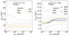Fig. B.2. Illustration of the NSS scheme used for cross-section nuisance parameters. Colour-coded solid lines correspond to existing cross-section parametrisations, W98 (Webber et al. 1998a,b,c), S01 (Soutoul, priv. comm.), W03 (Webber et al. 2003), and G17 (Moskalenko et al. 2001; Moskalenko & Mashnik 2003). Grey lines correspond to the median, 68%, and 95% confidence levels resulting from the use of NSS nuisance parameters, see Eqs. (B.1)–(B.3), taken from Table B.1.

Table B.1 lists the NSS μ and σ values used in the analyses described in the main text. In this analysis, the production cross-section reactions used correspond to cumulative cross-sections, i.e. the production of a given species Y accounting for all short-live fragments Y_i (decaying into Y):

$$\begin{array}{c}\hfill {\sigma }_{X+\mathrm{H}\to Y}^{\mathrm{c}}={\sigma }_{X+\mathrm{H}\to Y}+{\displaystyle \sum _i{\sigma }_{X+\mathrm{H}\to Y_i^{\star }}\times \mathcal{B}r(Y_i^{\star }\to Y).}\end{array}$$(B.4)

This is important to calculate correctly how much a reaction contributes to the total, as these number are used in Sect. 5.2.2 to interpret the post-fit values of the nuisance parameters. To be explicit, in Table B.1, the fraction given in square brackets for the production of ¹¹B and ¹⁵N account respectively for the significant contributions of the short-lived ¹¹C and ¹⁵O (Génolini et al. 2018).

Appendix C: Minimisation convergence

Many results in this work were obtained by fitting USINE V3.5 models to data, based on the MINUIT algorithm (James & Roos 1975). Because of the large number of free parameters in some configurations, it is important to check the reliability of the algorithm for finding the minimum of the χ² valley.

To do so, MINUIT was compared to two different minimisation algorithms. Technically, a python interface was implemented for χ² calls in USINE (this will be part of the next release), allowing the use of alternative algorithms from various python packages: (i) MINUIT (iMinuit package) is the state-of-the-art minimisation algorithm based on Migrad, which uses gradients to find the minimum of a scalar function, by iterative estimations of the Hessian matrix; (ii) Powell (SciPy package), does not rely on gradients, but uses iterative line searches instead, which are less prone to numerical instabilities that could arise in gradient calculations; (iii) the conjugate gradient (CG) method (SciPy package) is another gradient-based method that solves iteratively the linear algebraic problem of finding a minimum of a scalar function.

These three minimisers where tested on the same tasks and conditions, bookkeeping their performance and convergence over time, as measured by the number of χ² calls; the typical calculation time for one configuration is ∼𝒪(1 s), so that the number of calls is roughly the number of seconds. Their performance is shown in Fig. C.1 for a growing number of nuisance parameters in the analysis (from top to bottom). Two main conclusions can be taken from these plots. First, compared to the other algorithms (in blue and red), the MINUIT algorithm (in green) always provides the fastest route to the minimum. Second, with a larger number of parameters, i.e. a more complex parameter space, the chance of ending up in a local minimum increase (see bottom panel). No minimiser is immune to this, and the only option to overcome this difficulty is to use many trial starting points (represented by the many crosses).

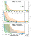Fig. C.1. Comparison of minimiser convergence speed and robustness. The dotted lines show the χ2 progress towards its minimum as a function of the number of calls, until the algorithm stops (cross symbol). Several algorithms are shown, namely Powell (blue), GC (red), and MINUIT (green), and the horizontal dash-dotted lines highlight the best-fit obtained for each algorithm. Ten different starting points are run, and the distribution of the best ${\chi }_{\text{min}}^2$ found are projected on the right-hand panel to show that sometimes the algorithm is stuck in a local minimum. From top to bottom: number of nuisance parameters in the model increases. See text for discussion.

From these tests, we conclude that MINUIT remains the best algorithm and that in order to find the true minimum, the minimisation must be repeated for 𝒪(100) different starting points, keeping the best χ² among all those obtained. This is the procedure we used for all the results presented in the main text.

Appendix D: Combining AMS-02 with lower-energy data

In this appendix, we explore the consistency of low-energy data (LE-data for short) with AMS-02 data, and we focus below on B/C data; the datasets used are detailed in Table D.1. These LE-data cover top-of-atmosphere (TOA) energies of 10 to 100 GeV/n. ACE-CRIS data are the most precise, with uncertainties at the level of ∼6%, i.e. only twice that of AMS-02. We do not consider in the following the recent Voyager 1 data covering a similar range in interstellar (IS) energies because our models do not match these data. This discrepancy was also observed in the analysis of Cummings et al. (2016), and whether this is an issue with the models, the cross-sections, specifics of the local interstellar medium, or even the data, which should be explored soon as Voyager 2 recently crossed into interstellar space (Stone et al. 2019), 6 years after Voyager 1, calls for a dedicated study that goes beyond the scope of this paper.

Figure D.1 shows the best-fit transport parameters and associated χ² for fits to B/C AMS-02 data only (large circles), or to B/C AMS-02 and LE-data together (small crosses). First, there is no impact for BIG because the model has too many low-rigidity competing transport parameters (break, η, and to some extent reacceleration and convection). Second, the impact is highest for the simplest model, SLIM, where the low-rigidity break value is better constrained with δ_l ≃ 1. Lastly, the situation is in between for QUAINT, with a slightly more constrained “low-rigidity” parameters η and V_a; moreover, because V_a couples to high rigidities, constraints on high-rigidity parameters are also slightly improved. We find similar trends for Li/C and Be/C (not shown).

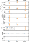Fig. D.1. Best-fit transport parameters and uncertainties for BIG, SLIM, and QUAINT (first, second, and third column) from B/C analysis. Large circles correspond to fits on AMS02 data only, whereas small crosses to the combined fits on AMS-02 and LE-data. Two bottom panels: ${\chi }_{\text{min}}^2/\text{d}.\text{o}.\text{f}.$ and ${\chi }_{\text{nui}}^2/n_{\text{nui}}$, defined in Eqs. (2) and (5), respectively.

Figure D.2 shows in the top panel the well-behaved residuals (within 1σ) of LE-data from the combined fit, while the bottom panel illustrates that the compatibility between LE-data and the model is not tapped in the extra nuisance parameters: the post-fit modulation levels, which cover solar minimum to solar maximum periods, all fall within 1σ of their input values, for all models (BIG, SLIM, and QUAINT). The same conclusions could have been directly read off the bottom panels of Fig. D.1: ${\chi }_{\text{min}}^2/\text{d}.\text{o}.\text{f}.$ decreases with LE-data (very good compatibility of LE-data with AMS-02 data) and ${\chi }_{\text{nui}}^2/n_{\text{nui}}$ only mildly increases.

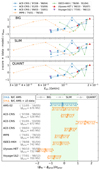Fig. D.2. Top panel: z-score = (model-data)/σdata of B/C LE-data used in the AMS and LE-data combined analysis for BIG (top), SLIM (middle), and QUAINT (bottom). To guide the eye, data points from the same experiments are linked. Bottom panel: post-fit residuals and 1σ uncertainty of the solar modulation nuisance parameters for BIG (solid lines), SLIM (dashed lines), and QUAINT (dash-dotted lines). The blue lines show the residuals for the fit to AMS-02 data only, and orange lines for AMS-02 and LE-data, one nuisance per dataset (per data-taking period). For comparison, the greenish vertical band shows the 1σ nuisance prior range.

Figure D.3 shows 1σ contours of the diffusion coefficient for B/C data in model BIG (top), QUAINT (middle), and SLIM (bottom). Compared to the analysis based on AMS-02 data only (blue solid lines, adding LE-data in the fit (purple dashed lines) strengthens the presence of a break for BIG and SLIM, but not for QUAINT; similar results are also obtained if relying on Li/C (or Be/C) instead of B/C data (not shown). For comparison purposes, we also show the contours obtained from combining Li/C, Be/C, and B/C (green dotted lines), as discussed in Sect. 3: this analysis now shows without ambiguity a break for all configurations.

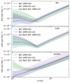Fig. D.3. Best-fit and 1σ contours for K(R) in BIG (top), SLIM (middle), and QUAINT (bottom) for three different analyses: fit to AMS-02 B/C data (blue contours), fit to AMS-02 B/C and LE-data (purple contours), and combined fit of AMS-02 Li/C, Be/C, and B/C data (green contours).

All Tables

All Figures

Fig. 1. Best-fit transport parameters with their asymmetric uncertainties (from MINOS) and corresponding ${\chi }_{\text{min}}^2/\text{d}.\text{o}.\text{f}.$ and ${\chi }_{\text{nui}}^2/n_{\text{nui}}$ (next-to-last and last panels) for BIG, SLIM, and QUAINT (first, second, and third column). Different secondary species are colour-coded, with different symbols for ratios to C (crosses) and to O (circles): “Be/C NoLE2” stands for Be/C AMS-02 data without the two lowest rigidity points (orange triangles), and LiBeB/C (or /O) stands for the combined analysis of Li/C, Be/C, and B/C (or /O). See text for details.

In the text

Fig. 2. Flux ratios (top), residuals (centre), and $\stackrel{\sim }{z}$-scores (bottom) for B/C (blue circles), Be/C (orange squares), and Li/C (green triangles). The models (top panel) are calculated for BIG (solid line), QUAINT (dash-dotted line), and SLIM (dotted line), from the best-fit transport parameters of the combined analysis of all three species. The residuals and $\stackrel{\sim }{z}$-score are shown for SLIM only; the $\stackrel{\sim }{z}$-score is related to the usual z-score by a rotation in a base where the covariance matrix of data systematics is diagonal (see text for details).

In the text

	Fig. 3. Best-fit and 1σ contours for K(R), see Eq. (1), reconstructed from the best-fit transport parameters (and their covariance matrix) from the combined LiBeB analysis. Three models are shown: BIG (orange), SLIM (green), and QUAINT (red). In the low-rigidity range, the factor β in Eq. (1) makes K(R) dependent on the CR species; shown are the result for A/Z = 2. See text for discussion.
In the text

Fig. 4. Propagation relative uncertainties (1σ contours with respect to median) as a function of rigidity based on the constraints set by the combined LiBeB analysis. Top panel: comparison of total transport uncertainties from BIG (solid), SLIM (dashed), and QUAINT (dash-dotted). Middle panel: separate uncertainty contributions from nuclear cross-sections (green), solar modulation (red), and transport (range) in SLIM. Bottom panel: comparison (in SLIM) of various calculated secondary-to-primary ratios within the combined LiBeB constraint.

In the text

Fig. 5. Best-fit transport parameters and uncertainties with the corresponding ${\chi }_{\text{min}}^2/\text{d}.\text{o}.\text{f}.$ and specific contribution from nuisance parameters (next-to-last and last columns) for different combinations of AMS-02 data: combined fit of LiBeB (red crosses); LiBeB and N/O combined (turquoise squares); LiBeB and 3He/4He combined (purple circles); LiBeB, 3He/4He, and N/O combined (brown triangles). From left to right: models BIG, SLIM, and QUAINT.

In the text

Fig. 6. Model calculation and data (first and second panel), residuals (third panel), and $\stackrel{\sim }{z}$-score (fourth panel) for N/O (turquoise circles), 4He (red squares), and 3He (pink triangles). For readability, He isotopic fluxes are multiplied by R2.2. Two top panels: model calculations for BIG, SLIM, and QUAINT along with their respective post-fit modulation level, two bottom panels: restricted to the best-fit configuration QUAINT. The inset shows the distance between the model and specific datasets, calculated from ${\chi }^2=\sum _i\stackrel{\sim }{z_i}$. All models are calculated from the best-fit parameters of the combined analysis of Li/C, Be/C, B/C, N/O, 3He, and 4He.

In the text

	Fig. 7. Distance (post-fit χ2) between data and models varying the correlation length ${\mathcal{l}}_{\rho }^{\text{Acc Rec}\&\text{Sel}}$ (in decades) of 3He and 4He data for QUAINT. The horizontal dotted line highlights the number of data points, indicating roughly the position at which χ2/d.o.f. ≈ 1.
In the text

Fig. 8. 3He/4He as a function of Ek/n for AMS-02 (purple squares) and PAMELA (green crosses)–the latter combine data from two different analysis, respectively PAMELA-ToF and PAMELA-Calorimeter (Adriani et al. 2016). All models are calculated from the best-fit parameters of the combined analysis of Li/C, Be/C, B/C, N/O, 3He, and 4He AMS-02 data. Different line styles show different model configurations (BIG, SLIM, and QUAINT) and their respective post-fit solar modulation level in purple. Green lines show the same model calculations but modulated at the PAMELA expected value of 539 MV.

In the text

Fig. 9. Correlations between the normalisation of the inelastic (left panels) or production (right panels) cross-sections and log10(K0), for models SLIM (top panels) and QUAINT (bottom panels). The various colours correspond to the normalisations of cross-sections involved in different CR species: Li (green), Be (orange), B (blue), N (turquoise), and 3He (crimson). The various symbols and line styles correspond to the post-fit values and ellipses (for the previously listed species) from various fit configurations: separate Li/C, Be/C, and B/C fits (“×” symbols and solid lines), combined Li/C, Be/C, and B/C fit (LiBeB for short, “+” symbols and dotted lines), combined LiBeB+N/O+3He+4He fit (“⋆” symbols and dashed lines). The horizontal grey dashed lines highlights the case of using unmodified cross-section datasets (T99 for inelastic and G17 for production, see Appendix B), i.e. ${\mathcal{N}}_{\mathrm{CR}}^{\mathrm{reac}.}=1$: the subscript in 𝒩 indicates the CR species associated with this nuisance parameter; the superscript shows the reaction used as a proxy for this CR. For production cross-sections (right panels), the normalisation parameters are not directly the value of the nuisance parameter, but are effective parameters, see Eq. (11). See text for discussion.

In the text

Fig. 10. Data (symbols) and model (lines) comparison for the most important production cross-sections leading to Li (top panel) and Be (bottom panel) fluxes. Their respective contribution to the total flux production is reminded in brackets. The data are taken from Génolini et al. (2018) and the model is the GALPROP parametrisation (Moskalenko et al. 2001; Moskalenko & Mashnik 2003). See text for discussion.

In the text

	Fig. A.1. Comparison of statistical and systematic uncertainties for N/O, B/C, Be/C, and Li/C (from thin to thick shaded lines). Values are taken from Aguilar et al. (2018a,b), except for “Acc. norm.”, “Acc. LE”, and “Acc. res.”, which are broken-down from Acc. uncertainties. See text for details.
In the text

	Fig. A.2. Correlation matrices colour-coded from zero (no correlation, white) to one (full correlations, blue). Three bottom panels: systematics whose amplitude are shown in Fig. A.1. Top right panel: correlation matrix from all acceptance uncertainties, top left panel: that from all uncertainties combined.
In the text

	Fig. A.3. Top panel: comparison of statistical and systematic uncertainties for 3He (thin lines) and 4He (thick lines) AMS-02 data. Bottom panel: correlation matrix for 3He (left) and 4He (right) as a function of R. All quantities are reconstructed from Aguilar et al. (2019); see text for details.
In the text

Fig. B.1. Impact of inelastic (left) and production (right) cross-section uncertainties on Li/C (first and third column) and Be/C (second and fourth column) ratio for specific reactions as a function of rigidity. In each panel the relative difference between (inelastic or production) cross-section parametrisations with respect to a reference one is shown in blue (associated with the right y-axis), whereas the impact on the calculated ratio (in model SLIM) of varying the cross-section is shown in black (associated with the left y-axis). To guide the eye, the vertical red line indicates the rigidity of the first AMS-02 data point. The bottom panels show the overall impact when all reactions (i.e. all nuclei in the network) are replaced. Inelastic cross-sections are B94 (Barashenkov & Polanski 1994), W96 (Wellisch & Axen 1996), T99 (Tripathi et al. 1996, 1999), and W03 (Webber et al. 2003). Production cross-sections are W98 (Webber et al. 1998a,b,c), S01 (Soutoul, priv. comm.), W03 (Webber et al. 2003), and G17 (Moskalenko et al. 2001; Moskalenko & Mashnik 2003).

In the text

Fig. B.2. Illustration of the NSS scheme used for cross-section nuisance parameters. Colour-coded solid lines correspond to existing cross-section parametrisations, W98 (Webber et al. 1998a,b,c), S01 (Soutoul, priv. comm.), W03 (Webber et al. 2003), and G17 (Moskalenko et al. 2001; Moskalenko & Mashnik 2003). Grey lines correspond to the median, 68%, and 95% confidence levels resulting from the use of NSS nuisance parameters, see Eqs. (B.1)–(B.3), taken from Table B.1.

In the text

Fig. C.1. Comparison of minimiser convergence speed and robustness. The dotted lines show the χ2 progress towards its minimum as a function of the number of calls, until the algorithm stops (cross symbol). Several algorithms are shown, namely Powell (blue), GC (red), and MINUIT (green), and the horizontal dash-dotted lines highlight the best-fit obtained for each algorithm. Ten different starting points are run, and the distribution of the best ${\chi }_{\text{min}}^2$ found are projected on the right-hand panel to show that sometimes the algorithm is stuck in a local minimum. From top to bottom: number of nuisance parameters in the model increases. See text for discussion.

In the text

Fig. D.1. Best-fit transport parameters and uncertainties for BIG, SLIM, and QUAINT (first, second, and third column) from B/C analysis. Large circles correspond to fits on AMS02 data only, whereas small crosses to the combined fits on AMS-02 and LE-data. Two bottom panels: ${\chi }_{\text{min}}^2/\text{d}.\text{o}.\text{f}.$ and ${\chi }_{\text{nui}}^2/n_{\text{nui}}$, defined in Eqs. (2) and (5), respectively.

In the text

Fig. D.2. Top panel: z-score = (model-data)/σdata of B/C LE-data used in the AMS and LE-data combined analysis for BIG (top), SLIM (middle), and QUAINT (bottom). To guide the eye, data points from the same experiments are linked. Bottom panel: post-fit residuals and 1σ uncertainty of the solar modulation nuisance parameters for BIG (solid lines), SLIM (dashed lines), and QUAINT (dash-dotted lines). The blue lines show the residuals for the fit to AMS-02 data only, and orange lines for AMS-02 and LE-data, one nuisance per dataset (per data-taking period). For comparison, the greenish vertical band shows the 1σ nuisance prior range.

In the text

	Fig. D.3. Best-fit and 1σ contours for K(R) in BIG (top), SLIM (middle), and QUAINT (bottom) for three different analyses: fit to AMS-02 B/C data (blue contours), fit to AMS-02 B/C and LE-data (purple contours), and combined fit of AMS-02 Li/C, Be/C, and B/C data (green contours).
In the text

References

- Adriani, O., Barbarino, G. C., Bazilevskaya, G. A., et al. 2013, ApJ, 770, 2 [NASA ADS] [CrossRef] [EDP Sciences] [PubMed] [Google Scholar]
- Adriani, O., Barbarino, G. C., Bazilevskaya, G. A., et al. 2016, ApJ, 818, 68 [NASA ADS] [CrossRef] [Google Scholar]
- Aguilar, M., Aisa, D., Alpat, B., et al. 2015a, Phys. Rev. Lett., 114, 171103 [CrossRef] [PubMed] [Google Scholar]
- Aguilar, M., Aisa, D., Alpat, B., et al. 2015b, Phys. Rev. Lett., 115, 211101 [NASA ADS] [CrossRef] [PubMed] [Google Scholar]
- Aguilar, M., Ali Cavasonza, L., Ambrosi, G., et al. 2016, Phys. Rev. Lett., 117, 231102 [NASA ADS] [CrossRef] [Google Scholar]
- Aguilar, M., Ali Cavasonza, L., Ambrosi, G., et al. 2018a, Phys. Rev. Lett., 120, 021101 [NASA ADS] [CrossRef] [PubMed] [Google Scholar]
- Aguilar, M., Ali Cavasonza, L., Alpat, B., et al. 2018b, Phys. Rev. Lett., 121, 051103 [CrossRef] [PubMed] [Google Scholar]
- Aguilar, M., Ali Cavasonza, L., Ambrosi, G., et al. 2019, Phys. Rev. Lett., 123, 181102 [NASA ADS] [CrossRef] [Google Scholar]
- Ahlers, M., & Mertsch, P. 2017, Prog. Part. Nucl. Phys., 94, 184 [NASA ADS] [CrossRef] [Google Scholar]
- Aloisio, R., Blasi, P., & Serpico, P. D. 2015, A&A, 583, A95 [NASA ADS] [CrossRef] [EDP Sciences] [Google Scholar]
- Barashenkov, V. S., & Polanski, A. 1994, Electronic Guide for Nuclear Cross Sections, Tech. Rep. E2-94-417, Comm. JINR, Dubna [Google Scholar]
- Berezhko, E. G., Ksenofontov, L. T., Ptuskin, V. S., Zirakashvili, V. N., & Völk, H. J. 2003, A&A, 410, 189 [NASA ADS] [CrossRef] [EDP Sciences] [Google Scholar]
- Berezinskii, V. S., Bulanov, S. V., Dogiel, V. A., & Ptuskin, V. S. 1990, in Astrophysics of Cosmic Rays, ed. V. L. Ginzburg (Amsterdam: North-Holland) [Google Scholar]
- Bernard, G., Delahaye, T., Keum, Y. Y., et al. 2013, A&A, 555, A48 [NASA ADS] [CrossRef] [EDP Sciences] [PubMed] [Google Scholar]
- Blasi, P., & Serpico, P. D. 2009, Phys. Rev. Lett., 103, 081103 [CrossRef] [PubMed] [Google Scholar]
- Blasi, P., Amato, E., & Serpico, P. D. 2012, Phys. Rev. Lett., 109, 061101 [NASA ADS] [CrossRef] [PubMed] [Google Scholar]
- Boella, G., Gervasi, M., Potenza, M. A. C., Rancoita, P. G., & Usoskin, I. 1998, Astropart. Phys., 9, 261 [NASA ADS] [CrossRef] [Google Scholar]
- Boschini, M., Torre, S. D., Gervasi, M., Vacca, G. L., & Rancoita, P. 2019, Adv. Space Res., 64, 2459 [NASA ADS] [CrossRef] [Google Scholar]
- Boschini, M. J., Torre, S. D., Gervasi, M., et al. 2020, ApJ, 889, 167 [NASA ADS] [CrossRef] [Google Scholar]
- Boudaud, M., Génolini, Y., Derome, L., et al. 2020, Phys. Rev. Res., 2, 023022 [CrossRef] [Google Scholar]
- Bouyahiaoui, M., Kachelriess, M., & Semikoz, D. V. 2019, JCAP, 2019, 046 [Google Scholar]
- Caballero-Lopez, R. A., & Moraal, H. 2004, J. Geophys. Res.: Space Phys., 109, 1101 [NASA ADS] [CrossRef] [EDP Sciences] [Google Scholar]
- Cholis, I., Hooper, D., & Linden, T. 2017, Phys. Rev. D, 95, 123007 [NASA ADS] [CrossRef] [Google Scholar]
- Coste, B., Derome, L., Maurin, D., & Putze, A. 2012, A&A, 539, A88 [NASA ADS] [CrossRef] [EDP Sciences] [PubMed] [Google Scholar]
- Cummings, A. C., Stone, E. C., Heikkila, B. C., et al. 2016, ApJ, 831, 18 [Google Scholar]
- Derome, L., Maurin, D., Salati, P., et al. 2019, A&A, 627, A158 [NASA ADS] [CrossRef] [EDP Sciences] [Google Scholar]
- di Bernardo, G., Evoli, C., Gaggero, D., Grasso, D., & Maccione, L. 2010, Astropart. Phys., 34, 274 [NASA ADS] [CrossRef] [EDP Sciences] [Google Scholar]
- Drury, L. O., & Strong, A. W. 2017, A&A, 597, A117 [NASA ADS] [CrossRef] [EDP Sciences] [Google Scholar]
- Dung, R., & Schlickeiser, R. 1990a, A&A, 237, 504 [NASA ADS] [Google Scholar]
- Dung, R., & Schlickeiser, R. 1990b, A&A, 240, 537 [NASA ADS] [Google Scholar]
- Duvernois, M. A., Simpson, J. A., & Thayer, M. R. 1996, A&A, 316, 555 [NASA ADS] [Google Scholar]
- Evoli, C., Blasi, P., Morlino, G., & Aloisio, R. 2018, Phys. Rev. Lett., 121, 021102 [NASA ADS] [CrossRef] [Google Scholar]
- Evoli, C., Aloisio, R., & Blasi, P. 2019, Phys. Rev. D, 99, 103023 [CrossRef] [Google Scholar]
- Feng, J., Tomassetti, N., & Oliva, A. 2016, Phys. Rev. D, 94, 123007 [CrossRef] [Google Scholar]
- Fisk, L. A., & Axford, W. I. 1969, J. Geophys. Res., 74, 4973 [NASA ADS] [CrossRef] [Google Scholar]
- Gabici, S., Evoli, C., Gaggero, D., et al. 2019, Int. J. Mod. Phys. D, 28, 1930022 [Google Scholar]
- Garcia-Munoz, M., Simpson, J. A., Guzik, T. G., Wefel, J. P., & Margolis, S. H. 1987, ApJS, 64, 269 [NASA ADS] [CrossRef] [EDP Sciences] [Google Scholar]
- Génolini, Y., Putze, A., Salati, P., & Serpico, P. D. 2015, A&A, 580, A9 [NASA ADS] [CrossRef] [EDP Sciences] [Google Scholar]
- Génolini, Y., Salati, P., Serpico, P., & Taillet, R. 2017a, A&A, 600, A68 [NASA ADS] [CrossRef] [EDP Sciences] [Google Scholar]
- Génolini, Y., Serpico, P. D., Boudaud, M., et al. 2017b, Phys. Rev. Lett., 119, 241101 [NASA ADS] [CrossRef] [PubMed] [Google Scholar]
- Génolini, Y., Maurin, D., Moskalenko, I. V., & Unger, M. 2018, Phys. Rev. C, 98, 034611 [NASA ADS] [CrossRef] [Google Scholar]
- Génolini, Y., Boudaud, M., Batista, P. I., et al. 2019, Phys. Rev. D, 99, 123028 [NASA ADS] [CrossRef] [Google Scholar]
- George, J. S., Lave, K. A., Wiedenbeck, M. E., et al. 2009, ApJ, 698, 1666 [Google Scholar]
- Ghelfi, A., Barao, F., Derome, L., & Maurin, D. 2016, A&A, 591, A94 [NASA ADS] [CrossRef] [EDP Sciences] [Google Scholar]
- Ghelfi, A., Barao, F., Derome, L., & Maurin, D. 2017a, A&A, 605, C2 [NASA ADS] [CrossRef] [EDP Sciences] [Google Scholar]
- Ghelfi, A., Maurin, D., Cheminet, A., et al. 2017b, Adv. Space Res., 60, 833 [NASA ADS] [CrossRef] [Google Scholar]
- Ginzburg, V. L., & Syrovatskii, S. I. 1964, The Origin of Cosmic Rays (New York: Macmillan) [Google Scholar]
- Gleeson, L. J., & Axford, W. I. 1967, ApJ, 149, L115 [NASA ADS] [CrossRef] [Google Scholar]
- Gleeson, L. J., & Axford, W. I. 1968, ApJ, 154, 1011 [NASA ADS] [CrossRef] [Google Scholar]
- Grenier, I. A., Black, J. H., & Strong, A. W. 2015, ARA&A, 53, 199 [NASA ADS] [CrossRef] [Google Scholar]
- Guo, Y.-Q., & Yuan, Q. 2018, Phys. Rev. D, 97, 063008 [NASA ADS] [CrossRef] [Google Scholar]
- James, F., & Roos, M. 1975, Comput. Phys. Commun., 10, 343 [NASA ADS] [CrossRef] [PubMed] [Google Scholar]
- Jóhannesson, G., Ruiz de Austri, R., Vincent, A. C., et al. 2016, ApJ, 824, 16 [NASA ADS] [CrossRef] [Google Scholar]
- Jones, F. C., Lukasiak, A., Ptuskin, V., & Webber, W. 2001, ApJ, 547, 264 [NASA ADS] [CrossRef] [Google Scholar]
- Kachelrieß, M., & Semikoz, D. V. 2019, Prog. Part. Nucl. Phys., 109, 103710 [CrossRef] [Google Scholar]
- Kachelrieß, M., Neronov, A., & Semikoz, D. V. 2015, Phys. Rev. Lett., 115, 181103 [NASA ADS] [CrossRef] [Google Scholar]
- Korsmeier, M., & Cuoco, A. 2016, Phys. Rev. D, 94, 123019 [NASA ADS] [CrossRef] [Google Scholar]
- Krombel, K. E., & Wiedenbeck, M. E. 1988, ApJ, 328, 940 [NASA ADS] [CrossRef] [Google Scholar]
- Lavalle, J., & Salati, P. 2012, C. R. Phys., 13, 740 [NASA ADS] [CrossRef] [Google Scholar]
- Lave, K. A., Wiedenbeck, M. E., Binns, W. R., et al. 2013, ApJ, 770, 117 [NASA ADS] [CrossRef] [Google Scholar]
- Lukasiak, A. 1999, Proceedings of the 26th International Cosmic Ray Conference. August 17–25, 1999. Salt Lake City, Utah, USA, 3, 41 [Google Scholar]
- Maurin, D. 2020, Comput. Phys. Commun., 247, 106942 [NASA ADS] [CrossRef] [Google Scholar]
- Maurin, D., Donato, F., Taillet, R., & Salati, P. 2001, ApJ, 555, 585 [NASA ADS] [CrossRef] [Google Scholar]
- Maurin, D., Taillet, R., & Donato, F. 2002, A&A, 394, 1039 [NASA ADS] [CrossRef] [EDP Sciences] [Google Scholar]
- Maurin, D., Putze, A., & Derome, L. 2010, A&A, 516, A67 [NASA ADS] [CrossRef] [EDP Sciences] [Google Scholar]
- Maurin, D., Cheminet, A., Derome, L., Ghelfi, A., & Hubert, G. 2015, Adv. Space Res., 55, 363 [NASA ADS] [CrossRef] [Google Scholar]
- Mertsch, P. 2018, JCAP, 2018, 045 [CrossRef] [Google Scholar]
- Mertsch, P., & Sarkar, S. 2014, Phys. Rev. D, 90, 061301 [NASA ADS] [CrossRef] [Google Scholar]
- Moskalenko, I. V., & Mashnik, S. G. 2003, Intern. Cosm. Ray Conf., 4, 1969 [NASA ADS] [Google Scholar]
- Moskalenko, I. V., Mashnik, S. G., & Strong, A. W. 2001, Intern. Cosm. Ray Conf., 5, 1836 [NASA ADS] [Google Scholar]
- Niu, J.-S., Li, T., & Xue, H.-F. 2019, ApJ, 873, 77 [NASA ADS] [CrossRef] [Google Scholar]
- Osborne, J. L., & Ptuskin, V. S. 1988, Sov. Astron. Lett., 14, 132 [NASA ADS] [Google Scholar]
- Perko, J. S. 1987, A&A, 184, 119 [NASA ADS] [Google Scholar]
- Picot-Clémente, N., Abe, K., Fuke, H., et al. 2015a, Intern. Cosm. Ray Conf., 34, 425 [Google Scholar]
- Picot-Clémente, N., Seo, E. S., Strong, A., & Lu, Y. 2015b, Intern. Cosm. Ray Conf., 34, 555 [Google Scholar]
- Picot-Clémente, N., Abe, K., Fuke, H., et al. 2017, Intern. Cosm. Ray Conf., 301, 210 [CrossRef] [Google Scholar]
- Putze, A., Maurin, D., & Donato, F. 2011, A&A, 526, A101 [NASA ADS] [CrossRef] [EDP Sciences] [Google Scholar]
- Reinert, A., & Winkler, M. W. 2018, JCAP, 2018, 055 [Google Scholar]
- Schlickeiser, R. 2002, Cosmic Ray Astrophysics (Berlin: Springer) [CrossRef] [Google Scholar]
- Schlickeiser, R., Jaekel, U., & Dung, R. 1991, A&A, 242, L5 [Google Scholar]
- Seo, E. S., & Ptuskin, V. S. 1994, ApJ, 431, 705 [NASA ADS] [CrossRef] [Google Scholar]
- Serpico, P. 2015, Intern. Cosm. Ray Conf., 34, 9 [NASA ADS] [Google Scholar]
- Serpico, P. D. 2018, J. Astrophys. Astron., 39, 41 [NASA ADS] [CrossRef] [Google Scholar]
- Shalchi, A. 2009, in Nonlinear Cosmic Ray Diffusion Theories (Berlin, Heidelberg: Springer-Verlag), Astrophys. Space Sci. Lib., 362 [Google Scholar]
- Stone, E. C., Cummings, A. C., Heikkila, B. C., & Lal, N. 2019, Nat. Astron., 3, 1013 [CrossRef] [Google Scholar]
- Thornbury, A., & Drury, L. O. 2014, MNRAS, 442, 3010 [NASA ADS] [CrossRef] [Google Scholar]
- Thoudam, S., & Hörandel, J. R. 2012, MNRAS, 421, 1209 [NASA ADS] [CrossRef] [Google Scholar]
- Tomassetti, N. 2012a, ApJ, 752, L13 [NASA ADS] [CrossRef] [EDP Sciences] [Google Scholar]
- Tomassetti, N. 2012b, Ap&SS, 342, 131 [CrossRef] [Google Scholar]
- Tomassetti, N. 2017, Phys. Rev. D, 96, 103005 [NASA ADS] [CrossRef] [Google Scholar]
- Tomassetti, N., & Donato, F. 2012, A&A, 544, A16 [NASA ADS] [CrossRef] [EDP Sciences] [Google Scholar]
- Tomassetti, N., & Oliva, A. 2017, ApJ, 844, L26 [NASA ADS] [CrossRef] [Google Scholar]
- Tripathi, R. K., Cucinotta, F. A., & Wilson, J. W. 1996, Nucl. Inst. Meth. Phys. Res. B, 117, 347 [NASA ADS] [CrossRef] [Google Scholar]
- Tripathi, R. K., Cucinotta, F. A., & Wilson, J. W. 1999, Nucl. Inst. Meth. Phys. Res. B, 155, 349 [NASA ADS] [CrossRef] [Google Scholar]
- Vittino, A., Mertsch, P., Gast, H., & Schael, S. 2019, Phys. Rev. D, 100, 043007 [CrossRef] [Google Scholar]
- Webber, W. R., Kish, J. C., Rockstroh, J. M., et al. 1998a, ApJ, 508, 940 [NASA ADS] [CrossRef] [Google Scholar]
- Webber, W. R., Kish, J. C., Rockstroh, J. M., et al. 1998b, ApJ, 508, 949 [NASA ADS] [CrossRef] [Google Scholar]
- Webber, W. R., Soutoul, A., Kish, J. C., et al. 1998c, Phys. Rev. C, 58, 3539 [NASA ADS] [CrossRef] [Google Scholar]
- Webber, W. R., Soutoul, A., Kish, J. C., & Rockstroh, J. M. 2003, ApJS, 144, 153 [NASA ADS] [CrossRef] [Google Scholar]
- Weinrich, N., Boudaud, M., Derome, L., et al. 2020, A&A, 639, A74 [NASA ADS] [CrossRef] [EDP Sciences] [Google Scholar]
- Wellisch, H. P., & Axen, D. 1996, Phys. Rev. C, 54, 1329 [NASA ADS] [CrossRef] [Google Scholar]
- Wu, J., & Chen, H. 2019, Phys. Lett. B, 789, 292 [NASA ADS] [CrossRef] [Google Scholar]
- Yang, R., & Aharonian, F. 2019, Phys. Rev. D, 100, 063020 [NASA ADS] [CrossRef] [Google Scholar]