| Issue |
A&A
Volume 668, December 2022
|
|
|---|---|---|
| Article Number | A7 | |
| Number of page(s) | 20 | |
| Section | Astrophysical processes | |
| DOI | https://doi.org/10.1051/0004-6361/202243446 | |
| Published online | 28 November 2022 | |
The importance of Fe fragmentation for LiBeB analyses
Is a Li primary source needed to explain AMS-02 data?
1
LPSC, Université Grenoble Alpes, CNRS/IN2P3, 53 avenue des Martyrs, 38026 Grenoble, France
e-mail: This email address is being protected from spambots. You need JavaScript enabled to view it.
2
Kapteyn Astronomical Institute, University of Groningen, Landleven 12, 9747 AD Groningen, The Netherlands
e-mail: This email address is being protected from spambots. You need JavaScript enabled to view it.
3
LAPTh, Université Savoie Mont Blanc & CNRS, Chemin de Bellevue, 74941 Annecy Cedex, France
e-mail: This email address is being protected from spambots. You need JavaScript enabled to view it.
4
Niels Bohr International Academy & Discovery Center, Niels Bohr Institute, University of Copenhagen, Blegdamsvej 17, 2100 Copenhagen, Denmark
Received:
1
March
2022
Accepted:
10
August
2022
Abstract
Context. High-precision data from AMS-02 on Li, Be, and B provide the best constraints on Galactic cosmic-ray transport parameters.
Aims. We re-evaluate the impact of Fe fragmentation on the Li, Be, and B modelling. We discuss the consequences on the transport parameter determination and reassess whether a primary source of Li is needed to match AMS-02 data.
Methods. We renormalised several cross-section parametrisations to existing data for the most important reactions producing Li, Be, and B. We used the USINE code with these new cross-section sets to re-analyse Li/C, Be/C, and B/C AMS-02 data.
Results. We built three equally plausible cross-section sets. Compared to the initial cross-section sets, they lead to an average enhanced production of Li (∼20 − 50%) and Be (∼5 − 15%), while leaving the B flux mostly unchanged. In particular, Fe fragmentation is found to contribute to up to 10% of the Li and Be fluxes. Used in the combined analysis of AMS-02 Li/C, Be/C, and B/C data, the fit is significantly improved, with an enhanced diffusion coefficient (∼20%). The three updated cross-section sets are found to either slightly undershoot or overshoot the Li/C and B/C ratios: this strongly disfavours evidence for a primary source of Li in cosmic rays. We stress that isotopic cosmic-ray ratios of Li (and to a lesser extent Be), soon to be released by AMS-02, are also impacted by the use of these updated sets.
Conclusions. Almost no nuclear data exist for the production of Li and B isotopes from Ne, Mg, Si, and Fe, whereas these reactions are estimated to account for ∼20% of the total production. New nuclear measurements would be appreciated and help to better exploit the high-precision AMS-02 cosmic-ray data.
Key words: astroparticle physics / diffusion / nuclear reactions, nucleosynthesis, abundances
© D. Maurin et al. 2022
 Open Access article, published by EDP Sciences, under the terms of the Creative Commons Attribution License (https://creativecommons.org/licenses/by/4.0), which permits unrestricted use, distribution, and reproduction in any medium, provided the original work is properly cited.
This article is published in open access under the Subscribe-to-Open model. This email address is being protected from spambots. You need JavaScript enabled to view it. to support open access publication.
1. Introduction
Galactic cosmic-ray (GCR) Li, Be, and B (hereafter LiBeB for short) isotopes are present in minute amounts in the Solar System, but are seen in excess in cosmic-ray (CR) data (e.g., Tatischeff & Gabici 2018). These CR species are denoted secondary species, as they are generally assumed to be produced only by a nuclear interaction of heavier CR species on the interstellar medium (ISM). The dominant channels for this production are the direct production of LiBeB from C and O CR fluxes (e.g., Génolini et al. 2018). The latter fluxes are among the most abundant CR species, and are of primary origin, that is they result almost solely from the diffusive shock wave acceleration of the ISM material. The study of secondary species, or secondary-to-primary ratios, plays a central role in CR physics because they calibrate the transport parameters in the Galaxy. The latter can give insight into the micro-physics of transport in the turbulent medium (e.g., Génolini et al. 2019), but it is also a central ingredient for many related studies (e.g., electron and positron spectra, γ-ray diffuse emissions, indirect searches for dark matter in CRs).
The AMS-02 experiment on board the International Space Station has collected an unprecedented number of CRs (Aguilar et al. 2021a); the data published by the collaboration reach the few percent level of precision. The LiBeB data, which display a spectral break at ∼200 GV (Aguilar et al. 2018a), have been used by several authors to study the transport of GCRs (Génolini et al. 2017, 2019; Evoli et al. 2019; Weinrich et al. 2020b; Boschini et al. 2020a,b; Yuan et al. 2020; De La Torre Luque et al. 2021a). The above studies assume no extra source of LiBeB, but it remains possible to have a small amount of secondary production inside the acceleration site (Mertsch et al. 2021; Kawanaka & Lee 2021), or even to have a primary source of Li (Kawanaka & Yanagita 2018) from nova explosions (Hernanz 2015).
All model calculations rely on a network of CR fragmentation reactions. Uncertainties on these reactions range from 10% to 20%, and are a limiting factor to take full advantage of the high-precision CR data (Génolini et al. 2018). For this reason, possible excesses or mismatches (between the model and the data) must be robustly checked against nuclear uncertainties (among others). A new methodology to account for and propagate these uncertainties was proposed in Derome et al. (2019). The main idea was to start from a given production nuclear dataset and, while fitting LiBeB data, to allow the most relevant reactions to vary around their central values; penalties prevent cross sections from wandering far away from their expected values and uncertainties. We successfully used this approach in Weinrich et al. (2020b) to show that models with a pure secondary LiBeB component give an excellent fit to the AMS-02 data, provided that a few cross-section values were varied by ∼15%; similar but independent studies reached the same conclusions (De La Torre Luque et al. 2021a,b; Korsmeier & Cuoco 2021). Conversely, Boschini et al. (2020b) recently argued for a hint of primary Li in CRs, though they do not exclude an overall bias in the Li production cross sections.
At a first glance, there is not much to do to improve the main LiBeB production channels. Indeed, comprehensive inspections of the nuclear cross-section parametrisations were carried out by several independent teams twenty years ago (Silberberg et al. 1998; Webber et al. 2003; Moskalenko et al. 2003; Moskalenko & Mashnik 2003), and were also re-inspected in more recent studies (Reinert & Winkler 2018; Evoli et al. 2018). However, a closer look shows that Evoli et al. (2018) only focussed on progenitors up to O, while Reinert & Winkler (2018) did so on those up to Si. This means that ‘recent’ nuclear data, for reactions involving nuclei heavier than Si (up to Ni), may have been skipped in this re-evaluation. The most comprehensive set of parametrisations, taking advantage of all nuclear data up to Ni, are those of Webber (Webber et al. 2003) and of the GALPROP team1. These parametrisations were, for instance, extensively used in Génolini et al. (2018) to rank the most important production channels for LiBeB; in these ranking, Fe (as a progenitor) only appears at the percent level. A closer inspection of the nuclear physics literature indeed indicates that important data, related to the fragmentation of Fe into LiBeB, only became available after these parametrisations were established; this means that Fe fragmentation into LiBeB must be re-evaluated.
This paper is organised as follows: in Sect. 2, we recall the setup used for the propagation and the motivation for our renewed interest in Fe fragmentation for LiBeB calculations. In Sect. 3, we gather and use available nuclear data to update cross-section parametrisations of the most important progenitors, highlighting the enhanced production of Li (with regard to Be and B) from Fe. In Sect. 4, we show a ranking of the most important progenitors of LiBeB, providing a complementary view of the rankings proposed in Génolini et al. (2018). In Sect. 5, we discuss the impact updated cross sections have on the derived transport parameters. In particular, we repeat and update our recent analysis of AMS-02 LiBeB data (Weinrich et al. 2020b), in order to address the interpretation of a primary source of Li in CRs. We also illustrate how isotopic ratios of Li, Be, and B fluxes (e.g., 6Li/Li and 7Li/Li) are sensitive to the uncertainties on the production cross sections. We then conclude in Sect. 6.
Additional comparisons and checks can be found in the appendices. Appendix A identifies the progenitors whose updated cross sections make up most of the observed changes in the Li/C, Be/C, and B/C ratios (hereafter LiBeB/C for short). Appendix B shows that the use of the new AMS-02 F, Ne, Na, Mg, Al, Si, and Fe data only marginally impact the LiBeB/C calculations, compared to our previous analysis (Weinrich et al. 2020b) in which only AMS-02 C, N, and O data were available. Appendix C shows the constraints set by the updated cross sections on various combinations of the transport parameters (only the simplest transport configuration is discussed in the main text).
2. Propagation setup and ingredients
2.1. CR flux calculation
The quasi-isotropic flux ψk(E) of a CR ion is related to its differential density Nk(E) by ψk = vNk/(4π), with Nk calculated from the transport equation (Berezinskii et al. 1990). In this study, we consider a 1D geometry (e.g., Maurin et al. 2022), with a thin plan (half-thickness h = 100 pc) in which the sources and the gas lie, hence where energy losses and nuclear reactions occur. We assume that CRs diffuse isotropically in a thick halo of half-size L, with a diffusion coefficient K(R); without loss of generality for our analysis, we set L = 5 kpc (Weinrich et al. 2020a,b). Further assuming steady-state, the transport equation in this geometry becomes a second order differential equation along the vertical spatial coordinate and on energy. To highlight the role of nuclear interactions, which are the prime focus of this study, we write below the (simplified) equation for our model (energy loss and gain terms, decay terms, and convective transport omitted):
![Mathematical equation: $$ \begin{aligned} -K \frac{\mathrm{d}^2 N^k}{\mathrm{d}z^2} =\! 2h\,\delta (z) \left[Q^k + \sum _{i\,\in \mathrm {ISM}} n_i\left(\sum _s v^s\,\!\sigma ^{s+i\rightarrow k}_{\rm prod}N^s -v^k\, \sigma ^{k+i}_{\rm inel}N^k\right)\right]. \end{aligned} $$](/articles/aa/full_html/2022/12/aa43446-22/aa43446-22-eq1.gif) (1)
(1)
The left-hand side term corresponds to diffusion, while the right-hand side has a primary source term, Qk(E), and two terms associated with nuclear interactions, written generically as ∑iniv σ(E). We use nISM = 1 cm3 (90% H and 10% He in number) and σ is a nuclear interaction, either corresponding to a net loss (destruction cross section σinel) or to a secondary source term (production cross section σprod, straight-ahead approximation assumed); the latter must sum over all possible CR progenitors s (heavier than the produced fragments of interest k). For CR elements below Ni, the above set of equations couples ∼100 species, which involves a nuclear network of ≳1000 reactions. The above coupled set of equations can be solved starting from the heaviest species – which is assumed to be a primary – and solving down to the lightest species. This ensures that all secondary contributions (from heavier species) are accounted for at each step k.
All the analyses presented below rely on the USINE package2 (Maurin 2020), and we stress that the analyses below solve the full transport equation, that is with energy gains and losses, decay terms, and possibly a constant convection term in the 1D geometry (Génolini et al. 2019)3. Inelastic cross-sections are an important ingredient of the calculation, but their uncertainties are subdominant in the total error budget (e.g., Génolini et al. 2019), so we do not discuss them in this paper; the parametrisation of Tripathi et al. (1997, 1999) are used.
2.2. Transport parameters
Even in the simple propagation framework used, transport parameters come in different flavours. For instance, Génolini et al. (2019) explored several configurations, with or without convection and re-acceleration, and different parametrisations of the diffusion coefficient K(R). It was found that several of them were able to give a very good fit to LiBeB data (Weinrich et al. 2020b). To ease the discussion and without loss of generality, most of our calculations will be carried out in the so-called SLIM configuration. The latter consists of pure diffusion (no convection, no reacceleration) with a break at both low- (Génolini et al. 2019; Vittino et al. 2019; Weinrich et al. 2020b) and high-rigidity (Génolini et al. 2017, 2019; Reinert & Winkler 2018; Niu & Xue 2020) in the diffusion coefficient:
 (2)
(2)
The high-rigidity break parameters Rh, δh, and sh are fixed to the values found in Génolini et al. (2019); we also enforce sl = 0.04. We stress that for the rest of this section, the other parameters are fixed to δl = −0.74, Rl = 4.53 GV, and δ = 0.51, K0 = 0.0389 kpc2 Myr−1 (Weinrich et al. 2020b). We later see in Sect. 5 how these parameters are impacted when re-analysing the LiBeB data with updated cross-section values. We also discuss how these results change with alternative convection and reacceleration models in Appendix C.
2.3. Nuclear cross sections: Relevance of Fe for LiBeB?
Production cross sections are the backbone of CR studies, and several parametrisations are publicly available from the GALPROP or USINE codes: (i) W03 (Webber et al. 2003) relies on an unreleased version of the WNEW code (Webber et al. 1998a,b,c), which is a semi-empirical parametrisation fitted on existing data; (ii) S01 (A. Soutoul, private communication) is very similar to W03 but with different parameters; (iii) Galp (Moskalenko et al. 2001; Moskalenko & Mashnik 2003) is based on systematic fits on existing nuclear data, where Galp-opt12 and Galp-opt22 pre-fit parametrisations come respectively from the 1998 version of the WNEW code or from the 2000 version of the YIELDX code (semi-analytical formulae fitted on data, Silberberg et al. 1998; Tsao et al. 1998). More details on all these parametrisations can be found in Génolini et al. (2018).
Many LiBeB/C recent studies considered CR progenitors up to Si at most (Reinert & Winkler 2018; Evoli et al. 2018; Génolini et al. 2019). Actually, most studies addressing a possible mismatch in the Li production considered parents up to Si (Weinrich et al. 2020b; Boschini et al. 2020b; De La Torre Luque et al. 2021b; Korsmeier & Cuoco 2021), and those considering progenitors up to Fe (Boschini et al. 2020a,b) relied on the Galp-opt12 production cross sections.
To highlight the importance of these different settings (cross-section set and heaviest CR parent considered), we show in Fig. 1 the relative difference between calculations of Li/C, Be/C, and B/C ratios (from top to bottom) performed with progenitors up to Fe, compared to a reference calculation with progenitors only up to Si. The various line styles and colours encode the use of the four cross-sections parametrisations discussed above, that is W03, S01, Galp-opt12, and Galp-opt22. The solid black lines (i.e., Galp-opt12) show that the choice of the heaviest progenitor (Fe instead of Si) has a marginal impact (≲3%) on all ratios, in line with checks that calculations up to Si are accurate enough to interpret LiBeB/C data (Maurin et al. 2001; Génolini et al. 2019). The use of S01 (dash-dotted blue) and W03 (dashed green) parametrisations lead to similar conclusions, though with a ∼5% increase of Be/B (middle panel); W03 does not provide production cross sections for Li. Only with Galp-opt22 (grey-dashed lines) do we see a significant and differential increase for Li/C (∼15%), Be/C (∼10%), and B/C (∼5%). A close inspection shows that large differences exist between specific reactions for these different parametrisations, in particular for the fragmentation of 56Fe into LiBeB isotopes.
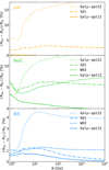 |
Fig. 1. Relative difference on Li/C (top), Be/C (middle), and B/C (bottom) between RFe (progenitors up to Fe, Z = 26) and RSi (progenitors up to Si, Z = 14) as a function of rigidity. The comparisons are carried out for four cross-section parametrisations available in the literature: Galp-opt22 (dotted lines), S01 (dash-dotted lines), W03 (dotted lines), and Galp-opt12 (solid lines). The enhanced production observed with Galp-opt22 motivates the re-analysis of the LiBeB production cross sections. |
This discrepancy, corresponding to an increased production of light nuclei in Fe fragmentation, might explain the mismatch seen in several analyses of Li CR data (Weinrich et al. 2020b; Boschini et al. 2020b; De La Torre Luque et al. 2021b; Korsmeier & Cuoco 2021). This clearly motivates a re-investigation of the nuclear data to see which of the above parametrisations is favoured by recent nuclear data.
3. Updating the LiBeB production cross sections
In this section, we review the wealth of nuclear data relevant for our study, briefly mentioning the different measurement techniques (Sect. 3.1). We then detail a procedure to update the cross-section parametrisations, highlighting the most impacted reactions (Sect. 3.2) and bracketing by how much Fe fragmentation impacts the LiBeB/C calculations (Sect. 3.3). In the rest of the paper, the original cross-section sets considered are the Galp-opt12 and Galp-opt22 parametrisations, and to avoid confusion, the new (updated) cross-section sets are denoted OPT12 and OPT22 respectively (a hybrid third set, OPT12up22, is also considered).
3.1. Nuclear data
Most of the nuclear cross sections relevant to CR studies are from the 1980s and 1990s, when it was realised that these inputs were essential to interpret elemental CR measurements. Back then, CR data were gaining in precision over a wider energy range, a situation quite similar to the one observed nowadays (with the advent of AMS-02, DAMPE, CALET, and PAMELA instruments). On the one hand, a wealth of nuclear data was provided by the Transport Collaboration (1990), who studied isotopic production cross sections through direct reactions, that is by measuring secondaries produced by ion beams (mostly Z < 26) colliding liquid hydrogen or carbon and methylene CH2 targets (and using a CH2 − C subtraction technique). This technique was notably used by Bill Webber and his colleagues, in the energy range ∼400–800 MeV/n (Webber & Brautigam 1982; Ferrando et al. 1988; Webber et al. 1990a,b,c,d, 1998a,b,c; Knott et al. 1996, 1997; Chen et al. 1997a,b). On the other hand, Michel and Leya’s group (Michel et al. 1989, 1995, 1997; Dittrich et al. 1990a; Bodemann et al. 1993; Sudbrock et al. 1996; Leya et al. 1998, 2005, 2006; Ammon et al. 2008) as well as Sisterson’s group (Sisterson et al. 1992, 1994, 1997, 2000; Sisterson & Caffee 1998; Kim et al. 2002; Sisterson & Vincent 2006) relied on indirect reactions, where a target of heavy elements is irradiated by a high-energy proton beam. With this technique, the cross sections are determined by γ-spectrometry whenever radioactive elements are produced, and after chemical processing by mass spectroscopy for the long-lived and stable isotopes. Although the target materials are generally not composed of pure isotopes, this technique gives a good approximation of the isotopic production cross sections from the dominant isotope in nature. We stress that this second technique does not directly provide the required cross sections, but must reconstruct the desired ones via measurements at different times (to account for the decay chain of short-lived nuclei) – see, for instance, Titarenko et al. (2008) and references therein for the steps to derive individual cross sections from cumulative ones.
The data collected for this work come from these two different techniques. Our starting point is the GALPROP cross-section database, assembled in the file isotope_cs.dat of the corresponding code4. We then performed extensive checks of the references therein–and also a few others pointed out in Reinert & Winkler (2018)–along with systematic extractions from the EXFOR database5 (Otuka et al. 2014). The reactions under scrutiny are those involving the most important progenitors of Li, Be, and B isotopes and ghosts (see below), that is (i) B, C, N, O, Ne, Mg, and Si, as highlighted in Génolini et al. (2018; ii) specific production of some light isotopes from Li and Be progenitors (for completeness of the Z ≤ 6 progenitors), and (iii) Fe which is the main novelty of this study. Indeed, new relevant fragmentation data from 56Fe (Napolitani et al. 2004; Herbach et al. 2006; Villagrasa-Canton et al. 2007; Titarenko et al. 2008, 2011) were published seemingly after the GALPROP database was last updated. Finally, our cross-checks lead us to replace some of the Read & Viola (1984) compiled data (used in the GALPROP file) by the original ones, and a few were even removed (because they corresponded to cumulative cross sections, i.e. with the contributions of short lives nuclei).
The updated dataset, for the specific channels leading to LiBeB, is more complete than the one used in Génolini et al. (2018). The data gathered are shown in Figs. 2–4. Despite these additional datasets, the reader can witness the scarcity of the data at energies relevant for GCRs studies (above GeV/n) and even the absence of data for some important channels. Recent reconsideration of this issue (Génolini et al. 2018) has already triggered a promising new experimental programme (Unger & NA61 Collaboration 2019) to improve the precision of these nuclear data and fill some of the gaps in existing measurements.
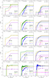 |
Fig. 2. Comparison of models and nuclear data for the fragmentation cross sections of 56Fe, 28Si, 24Mg, 20Ne, and 16O into Li (left), Be (centre), and B (right) isotopes and associated ghosts. The references for the data points are gathered in Fig. 5. |
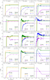 |
Fig. 3. Same as Fig. 2, but for 15, 14N, 12C, and 10, 11B progenitors. The references for the data points are gathered in Fig. 5. |
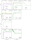 |
Fig. 4. Same as Fig. 2, but for and 10, 9, 7Be and 7Li progenitors. The references for the data points are gathered in Fig. 5. |
3.2. From data to updated parametrisations
Providing updated cross sections and the procedure to do so depends on three factors: the energy range we are interested in, the energy coverage of nuclear cross-section data, and the underlying model assumed for the production cross sections. The relevant energy range for AMS-02 data is a few GV to a few TeV/n, so that roughly, production cross sections of interest are in the GeV/n to TeV/n range. However, beside a few data points at 300 GeV/n (Raisbeck et al. 1975), and awaiting the promising new data at 13.5 GeV/n from the NA61/SHINE collaboration (Unger & NA61 Collaboration 2019; Amin & NA61/SHINE 2022), the bulk of nuclear data are below a few GeV/n. Furthermore, many reactions of interest for CRs are still lacking measurements or only have a few data points. In this context, very few reactions have a full coverage in energy, that is from tens of MeV/n (reaction threshold) up to multi-GeV/n, where it is generally assumed that the cross-sections become constant with energy. For this reason, it is necessary to have an underlying model to provide the cross sections for the missing reactions, or at least to provide an energy dependence to be normalised on the few existing data. This is in spirit close to the approach followed by the GALPROP team.
Of course, other approaches exist to improve, extend, and validate isotopic production cross sections (e.g. Boudard et al. 2013; Cheng & Feng 2021; Tao et al. 2021; Werneth et al. 2021; Dan et al. 2021). These works are more focussed on the microphysics. They also have a broader scope, in order to tackle a much larger variety of reactions and situations. However, they are not necessarily optimised for CR physics. For the time being, there is not a key advantage to using these other approaches, thus we rely here on updates and rescaling of the Galp-opt12 and Galp-opt22 parametrisations.
3.2.1. Procedure
After several trials and errors, we came up with a quite flexible procedure to update the production cross sections on hydrogen. This procedure proves to be quite successful in matching the data, in order to handle (i) the variety of situations for any given reaction (completeness or scarcity of data, discrepant data), (ii) the several energy regimes of the production process (steep rise at threshold, possible bumps and deeps, and asymptotically constant behaviour at high energy), and (iii) the fact that neither a simple rescaling of the Galp-opt12 and Galp-opt22 cross sections, nor a generic (and at the same time specific) enough formula can be satisfactorily used to fit all reactions. For any given reaction, this procedure goes in four steps detailed below.
Step 1: rescaling over the whole energy range. To do so, (i) we calculate the ratio r = data/model for the associated nuclear data; (ii) from these r, we form a spline 𝒮r that is used as an interpolation function (constant if used for extrapolation); (iii) we multiply the original model by 𝒮r. A logarithmic smoothing kernel (0.15 decade in energy) is then applied to ensure that the cross sections cannot have large variations on small energy scales6.
Step 2: dedicated fit for the low-energy rise. Near the reaction threshold, in order to reproduce the quick rise and possible bump, if enough data are available (typically > 6 data points), we directly fit a second order polynomial in
log − log scale enforcing convexity. This fit, that accounts for data uncertainties, replaces Step 1’s result in the low-energy regime.
Step 3: high-energy behaviour. Above 1.5 GeV/n, we consider two alternatives. We either keep the possible energy-dependant behaviour obtained at Step 1 (referred to as no-fit HE later on), or enforce a constant value based on a fit (accounting for data uncertainties) on existing data at these energies7. The latter configuration is taken as default, used throughout our paper, unless explicitly stated otherwise.
Step 4: scaling for He targets. Finally, not only cross sections on H matter, but cross sections on He (∼10% in number in the ISM) are also necessary. As a last step, we rescale the re-evaluated cross sections on H using the empirical formulae of Ferrando et al. (1988)8. These formulae, however, if naively applied, lead to arbitrarily large enhancements for the extrapolation to small fragments (in particular Li) and low energies, so that we enforce an ad hoc maximal enhancement (σHe/σH)max = 6. This can be compared to the few data points of Yashima et al. (2004), for the fragmentation of Z = 24 and Z = 26 into 7Be: at 100 (resp. 230 MeV/n), σHe/σH = 1.8 (resp. 2.0) for Cr, whereas σHe/σH = 17 for Fe9 (resp. 11). These measurements show irregularities that could probably not be captured by the scaling proposed by Ferrando et al. (1988). However, as will be seen later, the contribution of Fe fragmentation for the production of Li and Be reaches at most 10%: even a factor 3 error on the production of He (which is only 10% in number) would amount to a mere ≲3% bias on the total production; moreover, these enhanced production of light fragments only applies below a few hundreds of MeV/n, that is much below the range where AMS-02 collects data. Nonetheless, they might be of interest to interpret very low-energy Voyager data (Cummings et al. 2016).
3.2.2. Updated cross sections and most impacted reactions
As already said, we consider the most important CR progenitors for LiBeB production. We show the data and our new cross sections for the following CR isotopes: 56Fe, 28Si, 24Mg, 20Ne, and 16O progenitors in Fig. 2; then 14, 15N, 12C, and 10, 11B progenitors in Fig. 3; and finally 7, 9, 10Be and 7Li progenitors in Fig. 4. The legend and associated references for all the data presented are listed in Fig. 5.
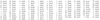 |
Fig. 5. References for all data points shown in Figs. 2–4, sorted from the most recent to the older ones. Specific labels from the original GALPROP files are [imos], [We96], and [NU98], which correspond to Igor Moskalenko’s additional data, Bill Webber private communication on Ramaty et al. (1997), and data retrieved from Nuclex (Ivanov et al. 1998) respectively. |
In Figs. 2, 3, and 4, the three columns (left, centre, and right) show the reactions related to the production of Li, Be, and B respectively. They include the direct production of stable (or CR-relevant) isotopes, but also the contributions from short-lived nuclei (dubbed ghosts), whose final decay state is one of these CR isotopes (Letaw et al. 1984; Maurin 2001): we recall that the cumulative cross-sections required for CR propagation corresponds to
 (3)
(3)
where ℬr (G → Y) is the branching ratio for the ghost G to end up as Y (see the third row of Table 1 for their values). In each panel of Figs. 2–4, the data (symbols) and updated models (OPT12 in thin lines and OPT22 in thick lines) are colour-coded according to the fragments considered. It is worth highlighting a few significant features: (i) when plenty of data exist, our procedure is very successful in matching the data at all energies; (ii) where only very few data exist, our procedure roughly amounts to a global rescaling of the initial cross sections; (iii) Galp-opt12 and Galp-opt22 parametrisations can have very different energy dependences, and these differences remain in OPT12 and OPT22 when only a few data are available (e.g., compare the thin and thick lines in the right-centre panel of Fig. 2, i.e. 24Mg in B through 11C); (iv) in several very relevant cases for which Galp-opt12 was null, the updated cross section OPT12 was replaced by a constant value passing through the few data points (e.g., top-left panel of Fig. 2, that is 56Fe in Li); (v) as already said, many reactions still lack any data (e.g., bottom-left panel of Fig. 3, that is 10Be in Li). We finally stress that for many reactions, Galp-opt12 and Galp-opt22 initial parametrisations were observed to be one and the same, so that their updated counterparts OPT12 and OPT22 are also one and the same; this peculiarity comes from the fact that these initial parametrisations were probably already rescaled to pre-2004 nuclear data for their use in GALPROP.
In order to have a more concise view of the main changes in these derived cross sections, we gather in Table 1 the ratio of the updated to initial cross sections above 1.5 GeV/n, ℛ = σupdated/σinitial, that is in a regime where we enforce the cross sections to be constant. The first column and first row respectively show the progenitors and fragments that appear in Figs. 2–4. The main comments we can make on this table are: (i) while data exist for the most important LiBeB contributors (C, N, and O, see Sect. 4), the less important Si, Mg, and Ne channels have no data at all for the production of Li and 10, 11B; (ii) contributions from the secondary species 10B and 7Be into Li – that peak at GeV/n energies, see Génolini et al. (2018) – also lack data; (iii) there is also no data for the production of 8He and 11Li ghost nuclei, however, owing to their small branching ratios and small cross-section predictions (compared to the other isotopes), these reactions are not expected to even reach the percent level of contribution overall; (iv) surprisingly, the initial cross sections Galp-opt12 and Galp-opt22 for the fragmentation of 12C and 16O into the short-lived 10C and 11C nuclei were null (a closer inspection indicates that these contributions were probably added to the direct production of 10Be and 11B); (v) the most striking numbers are those for the fragmentation of 56Fe, indicating that the initial Galp-opt12 (left-hand side numbers in the cells) significantly undershot the data, whereas the initial Galp-opt22 (right-hand side numbers in the cells) predictions were more or less in line with the data (with an overall small overshoot though). Looking back at Fig. 1, this latter behaviour seems to confirm and favour the case for an enhanced production of Li with regard to both Be and B (dotted lines).
Table 2 shows the ratio  , that is the comparison of two different choices for the high-energy update of the cross-section parametrisations: the numerator, ℛfit > 1.5 GeV/n, corresponds to the rescaling factors shown in Table 1 where cross sections are enforced to be constant above 1.5 GeV/n; the denominator, ℛno-fit, corresponds to the case in which the cross sections follow closely all structures seen in the high-energy data (see Sect. 3.2.1). This
  factors gives a hint of the variability of the data at high energy, and how sensitive the cross-section modelling is to these data. For readability, Table 2 only shows values significantly different from 1, that is reactions directly sensitive to this rescaling choice. We see that the fragmentation of 56Fe into Be isotopes and ghosts, and also that of 16O into Be and 10B, are significantly dependent on the two renormalisation procedure used. For a clearer illustration of this dependence, we show in Fig. 6 the production of Be from 56Fe (left panel) and 16O (right panel). The updated cross sections (thick coloured lines) clearly split above 1.5 GeV/n, and the case of σ16O + H→10Be illustrates the difficulty to favour one or the other approach, as the high-energy points are clearly below those at ∼1 GeV/n, though with much larger error bars. We also show on these plots the initial cross sections (thin black lines), to highlight the fact that moving from the old to the new cross sections is often more than a mere rescaling.
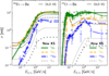 |
Fig. 6. Comparison of original (Galp-opt22, thin black lines labelled ‘OLD XS’) and updated (OPT22, thick coloured lines labelled ‘NEW XS’) production cross sections, for 56Fe (left) and 16O (right) fragmenting into Be isotopes. The two branches seen in some of the updated cross sections above 1.5 GeV/n illustrate two different procedures to update them (fit of a constant or spline passing through the data, see Sect. 3.2.1). The ratio of the values in these two branches at high energy corresponds to the values |

Ratio of high-energy rescaling factors between two methods tested,  , with ‘fit > 1.5 GeV/n’ for which the cross-section is constant above 1.5 GeV/n (fit on existing data and their errors) and ‘no-fit’ for which the model goes through all available points.
3.3. Impact on Li/C, Be/C, and B/C ratios
To start this subsection, we recall that we considered two different initial cross-section parametrisations, namely Galp-opt12 and Galp-opt22, rescaled to nuclear data and updated into OPT12 and OPT22. We also build a third cross-section set, where cross sections without data are taken from Galp-opt12, while those with data and updated are taken from OPT22; this hybrid configuration is denoted OPT12up2210.
We can now provide and bracket the impact these updated production cross sections have for the calculation of CR LiBeB/C ratios, as shown in Fig. 7. These curves tell us that heavy species up to Fe matter for the LiBeB production (see Fig. 1). As can be seen, whereas B is not impacted (≲4%) by the use of the updated cross-section sets, both Be and Li are significantly increased with regard to calculations performed with the original set Galp-opt12. These enhancements are also more important for Li than for Be, and this ordering holds true for the three updated cross-section sets. To better understand the origin of the increased production of Li and Be, we show in Appendix A the impact of individual progenitors. It confirms that Fe updated cross sections are the main driver of the Li and Be enhancements; the update of O and Si cross-sections is also contributing to this enhancement. More precisely, we can identify three different origins for the changes in the predicted (LiBeB)/C ratios, with the combined impact of (e.g., at 10 GV): (i) accounting for 56Fe fragmentation when moving from Galp-opt12 to Galp-opt22 that can be read off Fig. 1 (+15% for Li, +10% for Be, and +4% for B); (ii) renormalising Galp-opt22 into OPT22 for 56Fe reactions and other progenitors as read off the right panel of Fig A.1 (+6% for Li, +2% for Be, and −4% for B); (iii) accounting for the differing cross sections values for unmeasured reactions in Galp-opt12 and Galp-opt22. The latter is mostly significant for Li, as read off Fig. 7, indicating that the global change moving from Galp-opt12 to OPT12up22 can be even larger than the sum of the two first effects (+50% for Li, +10% for Be, and +2% for B).
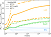 |
Fig. 7. Enhancement of Li/C (orange thick lines), Be/C (green lines), and B/C (blue thin lines) flux ratios with regard to calculations performed using Galp-opt12 (used in all recent studies). The three sets of curves correspond to the updated production cross-section sets OPT12 (dashed lines), OPT12up22 (solid lines), and OPT22 (dash-dotted lines). |
Concerning the spread between the OPT12, OPT12up22, and OPT22 sets in Fig. 7, we observe that the enhancement for Be is relatively well predicted (6% spread between the updated cross-section sets), while the spread on Li remains quite large (∼10 − 20%). This spread originates from the different values of the cross sections in the three updated sets. Indeed, for Fe, OPT22 (dash-dotted lines) provides a growing production cross sections with energy, whereas it is constant in OPT12 (see top left panel of Fig. 2). The difference between OPT12up22 (solid lines) and OPT22 (dash-dotted lines) is subtler and related to cross sections not rescaled: in the former set based on Galp-opt22 parametrisation, these cross sections are globally larger than in the latter set based on Galp-opt12. It is not clear whether the observed spread could be reduced by also applying our procedure to less-important cross-section reactions, or whether this difference is related to still unmeasured reactions; this certainly deserves further inspection. Finally, it is also difficult to decide which of the three updated cross-section sets proposed is the most motivated, all the more because, for the few reactions studied here and that were not renormalised to the data before, the cross sections from Galp-opt12 were found on average to undershoot the data, while those from Galp-opt22 to overshoot them (see Table 1).
4. Updated ranking for Li production
As underlined several times already, a thorough study and rankings of the most important reactions (or projectiles) involved in the production of Li to N fluxes were provided in Génolini et al. (2018). Owing to the important role of Fe fragmentation – that was not appreciated at that time – these ranking need to be updated. Instead of directly updating Tables V–VII and X–XII of Génolini et al. (2018), we provide a complementary view here, grouping contributions of specific CR elements. In words, for any given charge of a CR element Zi, we can track all the contributions leading directly or indirectly to Li, Be, or B. Mathematically-speaking, we can define the fi → j coefficients, which correspond to the fractional contribution of a CR isotope i ending up in a CR isotope j, via direct (1-step) or multi-step production. These coefficients read (see Eq. (A1) in Génolini et al. 2018)
 (4)
(4)
where i > k means that the CR isotope i is heavier than k. Denoting σij the cross section of i fragmenting in j (for any ISM target), the fi → j coefficients can be calculated from
 (5)
(5)
which by construction, ensures ∑ifi → j = 1. We can then define the fractional contribution fZi → Zj of a CR element of charge Zi into a CR element of charge Zj (with nZj isotopes) to be
 (6)
(6)
which also satisfies ∑ZifZi → Zj = 1.
Figure 8 shows from top to bottom, using OPT12up22, the quantities fZi → Li, fZi → Be, and fZi → B as a function of rigidity. Only progenitor elements having contributing fractions > 1% are shown, in order not to overcrowd the plot. As in Génolini et al. (2018), we recover that C and O are the main progenitors of Li, Be, and B, but at variance with these results, with the use of the updated cross-section sets, Fe can provide up to ∼10% of Li and Be (and ∼5% of B) at very high rigidity11. The remaining contributors are Mg, Ni, Ne, and N, that is the progenitors whose cross sections into LiBeB were updated in this study. We do not detail the multi-step production accounted for in the above plot. For instance, for Li, it amounts to ≲15% of the total production and peaks at at few GV (Génolini et al. 2018). Among the important two-step reactions for the production of Li, one finds 16O→11B→7Li (∼1.5%), for which the two associated production cross sections are already updated in our procedure. However, for some others, like the first ranking two-step reaction 16O→15N→7Li (∼1.9%), only one cross section is updated. It is not straightforward to quantify the benefit one would get by renormalising also the relevant cross sections for the most important two-step production channels. It should be a subdominant correction, but updating these cross sections should nevertheless be part of the global strategy to improve the CR flux predictions.
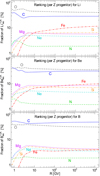 |
Fig. 8. Colour-coded ranked progenitors (elements) of the Li, Be, and B (from top to bottom) fluxes as a function of rigidity. Calculations are based on OPT12up22 production cross-section set with fluxes modulated at 700 MV. For readability, only contributing fractions larger than 1% are shown. |
We finally comment on the rigidity dependence of the contributing fractions seen in Fig. 8. We recall that the heavier the species, the larger the inelastic cross section, implying a more damped flux at low rigidities (when the interaction rate is larger than the diffusion rate). As a result, ratios of heavier-to-lighter primary CRs, while asymptotically constant at high energy (we assume the same injection spectrum for all species heavier than C here), decrease with decreasing energy below a few tens of GeV/n; this behaviour was highlighted in Fig. 14 of Putze et al. (2011) and is also seen in the recent AMS-02 Fe/O data (see Fig. 3 of Aguilar et al. 2021b). Coming back to Fig. 8, heavy elements represent a growing fraction of the total CR species with growing energy, and this explains why the contributing fraction of Fe in LiBeB (red dash-dotted curves) grows with energy12, with respect to C and O contributions.
5. Consequences of the updated cross sections: LiBeB/C re-analysis
To assess the impact of using the updated production cross-section sets, we re-analyse the AMS-02 LiBeB/C data. We stress that throughout this section, the cross sections used for the propagation runs are the cumulative ones. These cumulative production cross-section sets are generated from the individual reactions, following Eq. (3). We thus have three sets of cumulative cross sections that we keep denoting OPT12, OPT12up22, and OPT22 for simplicity.
Methodology. We repeat below the analysis of Weinrich et al. (2020b), which is based on AMS-02 Li/C, Be/C, and B/C data from 2011 to 2016 (Aguilar et al. 2018a)13. In detail, we perform a χ2 analysis with the MINUIT minimiser (James & Roos 1975), where χ2 values are obtained from the sum over (i) the quadratic distance between the model and data, accounting for a covariance matrix 𝒞 of data uncertainties (Derome et al. 2019; Génolini et al. 2019; Weinrich et al. 2020b); (ii) a Gaussian-distributed nuisance parameter 𝒩ϕ for the Solar modulation Fisk potential ϕ (Gleeson & Axford 1967, 1968) with mean μϕ = 676 MV (appropriate for the LiBeB data taking period) and σϕ = 100 MV (Weinrich et al. 2020b; iii) a series of Gaussian-distributed nuisance parameters  associated to a selection of LiBeB production reactions (Derome et al. 2019; De La Torre Luque et al. 2021b; Korsmeier & Cuoco 2021); the latter parameters combine a shift in the normalisation and a tilt on the slope of the cross sections, as introduced in Derome et al. (2019). Formally, this leads to
 (7)
(7)
where r runs over the nr cross-section reactions used as nuisance (see below). It is also useful to isolate the specific contribution of the nuisance parameters to the total χ2, that is
 (8)
(8)
which tells us how far away from our initial guess the post-fit values are. We recall that a good fit of the model to the data typically correspond to  and should have
  (i.e., nuisance parameters within 1σ of their central values on average).
Post-fit values μpfor cross-section nuisance parameters. The selection of a few most impacting cross sections to use as nuisance are the same as in Weinrich et al. (2020b)14 and they only involve reactions on H targets. For the inelastic interactions the most impacting reactions for LiBeB are 12C+H, 7Be+H, and 11B+H. The production reactions are however the most impacting ones: for each element considered in the analysis, we associate a single proxy reaction p, related to the production of an isotope (of this element) from the most impacting progenitor. For Li, Be, and B studied here, the associated proxies are p(Li) = 16O + H → 6Li, p(Be) = 16O + H → 7Be, and p(C) = 12C + H → 11B. This means that in order to obtain a good fit to LiBeB/C, the associated proxy cross-section values σp were renormalised into μp × σp, where μp are the post-fit values.
We stress that using a single isotopic cross section as a proxy to account for the uncertainties in an element production is mandatory to avoid degeneracies that would appear, were several isotopic cross sections used for the same element (Derome et al. 2019). However, an undesired side-effect of using a single proxy is that it biases the prediction of isotopic fluxes and ratios. As we want to use the post-fit values of these proxies to draw conclusions about the need for primary source terms for LiBeB, and also to make predictions for future isotopic ratios measured by AMS-02, these proxies must be handled with care.
Contributing fractionsfrfor relevant reactions. We recall that a given reaction r (from a CR progenitor into a CR fragment) only contributes to a fraction fr of the overall element production (from all possible CR progenitors). For the Li, Be, and B elements, these fractions have been calculated in Génolini et al. (2018). We report below, for each proxy p considered, the fr associated to that proxy (in boldface) and also to the other isotopes (for the element involved)15, that is
 (9)
(9)
From μpto global production correction  . When considering a secondary species Z, we can calculate a global correction factor to apply for the overall production of the element Z (from any progenitor), as opposed to the single correction μp applied on the proxy p (i.e., single progenitor into a single isotope). We would obtain exactly the same secondary-to-primary elemental ratio (as with the single proxy reaction correction) when applying the correction factor
  to all individual production cross sections into isotopes of the element Z. This global correction factor
  is obtained from
 (10)
(10)
The benefit of this procedure is that the global factor  now directly tells us by how much the overall production of an element must be modified to match the data: if
  > 1 (resp. < 1), the overall production must be larger (reps. smaller) that what we assumed in the production cross-section set. Considering, for instance, B with its proxy p=12C + H→11B, assuming μp = 1.2 and applying the above equation would give
  = (1.2 − 1)×33%+1 = 1.067. This would mean that overall, the production reactions of B are off and must be increased by 6.7% to match AMS-02 LiBeB/C data. The
  values are used for the discussion about evidences for LiBeB primary source terms in Sect. 5.2.
Unbiased isotopic production cross sections via μiso. Applying a correction on the proxy reaction only (e.g., μp=12C + H→11B = 1.2 in the above example) changes the predictions for CR isotopic ratios without real justification. To avoid this, one possibility is to redistribute this modification democratically between the isotopes (e.g., 10B and 11B here). In practice, we build new production cross-section sets (from our updated sets), applying the correction factor  for all reactions from the progenitor (used in the proxy) into the isotopes of the element (to which the proxy is associated), with
 (11)
(11)
For instance, the proxy p=12C + H→11B involves the progenitor 12C, so that using the above equation, we apply the correction  = [(1.2 − 1)×33%]/43%+1 = 1.15516 to both the cross sections σ12C + H→10B and σ12C + H→11B (instead of using the single proxy correction μp × σ12C + H→11B). These new sets are identified by the suffix ‘-U’ (for unbiased) – that is we build OPT12-U, OPT12up22-U, and OPT22-U – and are used for isotopic ratio calculations in Sect. 5.3; and we explicitly checked that these sets leave unchanged the predictions for the elemental fluxes (as expected).
Now that we are done with the definitions, we can move on to the interpretation of our LiBeB/C re-analysis results: first, we discuss the impact of the new cross-section sets OPT12, OPT12up22, and OPT22 on the transport parameters (Sect. 5.1); second, we address the need for a primary lithium source (Sect. 5.2); finally, we study the impact of the updated cross-section sets on CR isotopic ratios (Sect. 5.3).
5.1. Impact on transport parameters
In this subsection, we show the constraints set on the SLIM parameters at L = 5 kpc (see Appendix C for the constraints on BIG and QUAINT). The minimisations involve 7 nuisance parameters (one for Solar modulation and 6 for cross sections) and 201 LiBeB/C data points. We show in Fig. 9 the best-fit transport parameters of SLIM, that is, from top to bottom, the normalisation and slope of the diffusion coefficient (K0 and δ), and the low-rigidity break parameters (δl and Rl, see Eq. (2)) for different cross-section sets; the next-to last and last panels show  and
and  respectively, see Eqs. (7) and (8). We show on the right-hand side of the plot the values obtained in this analysis with the three updated cross-section sets OPT12, OPT12up22, and OPT22. For comparison purpose, we also report, on the left-hand side of the plot, the parameters obtained in Weinrich et al. (2020b) from the same LiBeB analysis but with the original set Galp-opt12 (violet stars), and those obtained even earlier from the same cross-section set in Génolini et al. (2019) where only a fit to AMS-02 B/C data was performed17 (cyan crosses). The latter result is shown to recall that, with respect to a combined analysis of several secondary-to-primary species, the analysis of a single ratio is both less constraining (larger error bars) and possibly biased by systematics in the production cross sections (Derome et al. 2019; Weinrich et al. 2020b).
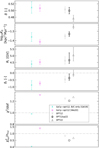 |
Fig. 9. Best-fit transport parameters (and uncertainties) from the fit to AMS-02 LiBeB/C data using different cross-section sets: from left to right, the original Galp-opt12 set used in Génolini et al. (2019) and Weinrich et al. (2020b), and the three updated sets obtained in this paper (OPT12, OPT12up22, and OPT22). The next-to-last and last panels show the |


The striking features seen in Fig. 9 for the combined LiBeB/C fit are the following. Firstly, when going from OPT12 to OPT22, the normalisation K0 (second panel) grows, whereas the low-rigidity break δl becomes consistent with 0 (i.e., no break). The change in K0 is directly linked to the updated cross sections, as more production means less grammage to produce the same amount of secondary species, which in turns means a larger diffusion coefficient (at fixed halo size L). The overall impact on the diffusion coefficient K(R) is also illustrated in Fig. 10 where 1σ envelopes are shown.
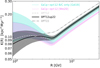 |
Fig. 10. Best-fit and 1σ envelopes for the diffusion coefficient, Eq. (2), associated to the parameters shown in Fig. 9 and for the same cross-section sets (L = 5 kpc). For readability, we do not show the envelopes for OPT12 and OPT22 as they are similar to those for OPT12up22. |
Secondly, not only do the updated cross-section sets improve the global fit substantially, but they also reduce the deviations of the nuisance parameters from their priors. In particular, the best χ2/d.o.f. is obtained for OPT12up2218 (black circle), with a very significant improvement ( goes from 258.3 to 237.5) compared to the use of the original Galp-opt12 set in Weinrich et al. (2020b) analysis (violet star). This OPT12up22 set also gives the smallest
  value, making it the most favoured by the LiBeB/C data.
For illustration purpose, the best-fit models for Li/C, Be/B, and B/C ratios are reported (SLIM configuration for the various cross-section sets) and compared to the data in the top panel of Fig. 11. For the specific OPT12up22 cross-section set, we further show in the middle and bottom panels respectively, the residuals with regard to the total uncertainties (systematics and statistic combined) and the rotated score  ; the latter quantity accounts for the role of correlations in the data systematics19. Overall, the above plot is very similar to the corresponding one shown in Fig. 2 of Weinrich et al. (2020b), that is the model matches the data quite well. Moreover, very similar χ2/ndata values (as reported in the legend of the second panel) and goodness-of-fit are obtained for the BIG and QUAINT configurations (not shown).
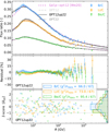 |
Fig. 11. Flux ratios (top), residuals (centre) and |


5.2. Is a primary source of Li needed?
We recall that in Boschini et al. (2020b), using the propagation code GALPROP and no nuisance parameters on the cross sections, the authors proposed the presence of a primary Li contribution to correct for a 20–25% deficit between the model and the data. Conversely, using nuisance parameters and relying on the same cross-section set Galp-opt12, Weinrich et al. (2020b) found no mismatch between the model and the data, but rather the need for a 13% increase of the production cross section of Li (see also De La Torre Luque et al. 2021a,b, for similar conclusions, though with slightly different numbers). The latter conclusion was reached by inspecting  values calculated from Eq. (10), reproduced here with star symbols (and their associated ellipses) in the left-hand side of Fig. 12: in Weinrich et al. (2020b)’s analysis, to match the LiBeB/C data with the Galp-opt12 cross-section set, the overall production of Li had to be increased by 13%, and that for B (resp. Be) had to be decreased by 3% (resp. 6%).
 |
Fig. 12. Correlation between log10(K0) and the normalisation factor |

This picture changes when considering our updated cross-section sets: moving from the original Galp-opt12 to the updated sets (from left to right in the plot), the total Li production goes from a significant increase (+13%) to a mild decrease (−5%), whereas the total B production evolves in the opposite direction (from −3% to +10%); the overall production of Be remains stable at ∼ − 5%. This shows that there is no need for a primary source of Li, and that we cannot trust the fact that, taken at face value, we would need now a primary source of B. Our analysis merely reinforces the conclusions of Weinrich et al. (2020b) and De La Torre Luque et al. (2021a): AMS-02 LiBeB/C data can be reproduced without invoking the presence of a new primary source because mismatches are likely to be associated to cross-section uncertainties. We also note in passing that OPT12up22, which was our (slightly) favoured configuration from the nuclear data perspective (see Sect. 3.2), is the one that best-fit AMS-02 LiBeB/C data (see Fig. 9). It is also the one for which  values are the closest to 1 (within ±5%, see empty circles in Fig. 12), that is minimal modifications needed for the production cross sections.
Figure 12 and the discussion are based on the SLIM configuration, but we checked that the BIG and QUAINT configurations lead to the same decrease/increase of the Li, Be, and B production cross sections (and their uncertainties), that is same values as those shown in Fig. 12 along the y axis. Our conclusion against the evidence of a Li primary source in CRs is thus independent of the propagation configuration and robust.
5.3. Impact on isotopic ratios
It is also interesting to see whether the updated cross-section sets predict different isotopic contents for the LiBeB elements. The HELIX project (Park et al. 2019) and the AMS-02 (Aguilar et al. 2019) experiment both have the capability to separate light isotopes from a few hundreds of MeV/n up to ∼10 GeV/n, whereas past experiments only provide data on a much limited range; the most recent data on Z = 3 − 5 isotopic fluxes are from ACE (de Nolfo et al. 2006), AMS-01 (Aguilar et al. 2011), ISOMAX (Hams et al. 2004), and PAMELA (Menn et al. 2018; Nozzoli & Cernetti 2021).
We show in Fig. 13 various isotopic ratios of Li, Be, and B, calculated from the best-fit models (parameters shown in Sect. 5.1) for various ‘unbiased’ production cross-section sets. We see that the updated sets predict very similar isotopic ratios for all species, except for Li isotopes, for which the largest difference is seen for 7Li/6Li; this is not so surprising since all sets were renormalised to the same nuclear data (though the underlying original cross-section models have different energy dependences, and possibly different prediction for unmeasured reactions). The largest difference for 7Li/6Li is at high energy and disappears at low energy. It is likely to be associated with Fe fragmentation: as seen in Fig. 8, the contribution from Fe to the total production vanishes at low energy, and as seen on the top left panel of Fig. 3, this is where the updated cross-section values differ most for both 6Li and 7Li. The difference between Galp-opt12 (dashed lines) and the updated cross-section sets (all other lines) is also maximal for Li isotopes: the origin of the difference can be read off Table 1, where one can see that the production cross sections from 16O and 12C have been increased for 6Li and decreased for 7Li. The differences seen for the other isotopes are smaller, but also result from the updated cross sections listed in Table 1. This behaviour is qualitatively (but not quantitatively) the same if we consider the BIG and QUAINT transport configurations instead of SLIM.
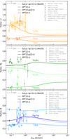 |
Fig. 13. Isotopic ratios of Li, Be, and B (from top to bottom panel) calculated from the best-fit models to AMS-02 LiBeB/C (at fixed L = 5 kpc). The production cross-section sets considered are the original Galp-opt12 (dotted lines) and the updated sets OPT12 (dashed lines), OPT12up22 (solid lines), and OPT22 (dash-dotted lines); the suffix ‘-U’ in the labels recalls that we use here unbiased cross-section sets, see Eq. (11). The data are from IMP (Garcia-Munoz et al. 1977a,b, 1981), Balloon ’73/08 (Hagen et al. 1977), Balloon ’77/05 (Buffington et al. 1978), Balloon ’77/09 (Webber & Kish 1979), Balloon ’70/06 (Bjarle et al. 1979), ISEE3 (Wiedenbeck & Greiner 1980; Mewaldt et al. 1981; Krombel & Wiedenbeck 1988), HEIST (Gibner et al. 1992), Ulysses (Connell 1998), Voyager1&2 (Lukasiak 1999), SMILI-II (Ahlen et al. 2000), ISOMAX (Hams et al. 2004), ACE (Yanasak et al. 2001; de Nolfo et al. 2006), AMS-01 (Aguilar et al. 2011), PAMELA (Menn et al. 2018; Nozzoli & Cernetti 2021). |
We finally want to stress that the suffix ‘-U’ in the labels of Fig. 13) indicate that our predictions were made with the ‘unbiased’ cross-section sets. In these sets, the corrections applied to cross-sections for a given element are distributed equally between the various isotopes of this element – parameter μiso in Eq. (11). We recognise that this procedure is debatable. Indeed, once the fitting procedure to secondary elements decides that the overall production of the said element must be slightly increased (or decreased), there is no real clear path to choose how to distribute this modification over the various isotopes (i.e., modification of a specific isotope or equally distributed between isotopes). Using more proxy reactions (e.g., one proxy per isotope) must be backed-up by isotopic ratio data in the fit, otherwise the various proxy parameters are degenerated; in that latter case, post-fit value would have no predictive power and would lead to overestimated variations in the predicted isotopic ratios. As illustrated in Fig. 13, current data (symbols) are clearly too scattered and imprecise to get a stronger handle on the isotopic production cross sections. Moreover, at this stage, it is difficult to quantify whether our updated (and ‘unbiased’) cross-section sets provide an improvement over the use of the original Galp-opt12-U set. The forthcoming AMS-02 and HELIX data are awaited to make some progress on these issues.
6. Conclusions
We have revisited and updated the production cross sections of Li, Be, and B species. We showed that contributions from Fe favour an enhanced production of Li – and to a lesser extent Be – with respect to B. We emphasised that most (and possibly all) previous interpretations of the AMS-02 Li, Be, and B data rely on a cross-section set that does not account for these enhancements. The consequences of using updated cross sections are the following20: (i) in the ranking of the most important progenitors for LiBeB, Fe becomes the third most important element, responsible for ∼10% of Li and Be21, but only ∼4% for B; (ii) the combined analysis of the AMS-02 Li/C, Be/C, and B/C ratios lead to a 20% larger value of the diffusion coefficient (compared to those obtained in our previous investigation), which is not without consequences for the predictions made, for instance, on secondary antiprotons (Boudaud et al. 2020)22; (iii) the updated cross-section sets also impact the predictions for the isotopic ratios of Li, Be, and B – in particular, uncertainties on the production of Be isotopes may be an issue for the determination of the halo size of the Galaxy (see the companion paper, Maurin et al. 2022); (iv) via the inspection of the post-fit values of the nuisance parameters (on the production cross section), we find that the updated cross-section sets, expected to be closer to the truth, indeed provide a more consistent description of the Li/C, Be/C, and B/C data – this is reassuring and validates to some extent our approach.
We recall that the motivation for this re-analysis was the interpretation of a mismatch between models and AMS-02 Li data, interpreted by some authors as a possible hint for a primary source of Li. We unambiguously showed here that the need for an extra Li component completely disappears, comforting the studies arguing for systematics in the production cross sections instead; at variance with these studies, however, we showed that these systematics were mostly attributed to an underestimated production of Li from Fe. Actually, the different plausible cross-section sets we built either lead to the need for a 5 − 10% increase or decrease of Li and B production cross sections; our favoured cross-section set (that also happens to provide the best-fit to Li/C, Be/B, and B/C data) even leads to a very small excess of Li with respect to the data. For this reason, we caution against any hasty interpretation of these overshoots or undershoots: they merely reflect the presence of systematics or still missing important reactions in the production cross-section sets.
The next step of this work would be to generalise our normalisation procedure (on nuclear data) to sub-dominant production channels. It could also be useful to make systematic comparisons to state-of-the-art cross-section codes like SPACS (Schmitt et al. 2014), FRACS (Mei 2017), or others, in order to better quantify systematics related to unmeasured cross sections. The rescaling procedure should then be extended to the production of secondary species with Z > 5, as all the elements up to Fe are within reach of the AMS-02 experiment. On the nuclear data side, new measurements for the production of Li and B isotopes from C and O, but also from Ne, Mg, Si, and Fe progenitors would be of great value: these progenitors amount to ∼20% of the total production of Li and B, while many of these reactions remain unmeasured or with only a couple of data points.
The same model and approach was used in several of our previous analyses of AMS-02 B/C and LiBeB/C nuclei (Génolini et al. 2017, 2019; Weinrich et al. 2020b), and we refer readers to these publications for more details.
This smoothing cures situations of nearby discrepant data points, while its main drawback is to slightly shift the threshold energy of the reaction to higher energy if there are no data; otherwise see Step 2.
We chose 1.5 GeV/n in order to have one or multiple points to fit a constant, but this is far from being an ideal choice, in a region where some energy dependence might remain – see the prediction of the WNEW code in Fig. 5 of Webber et al. (2003) as an illustration. In any case, the residual dependence of the models is generally within the nuclear data uncertainties (see the same figure in Webber et al. 2003). Waiting for more data in this energy range, using 1.5 GeV/n or a higher value (e.g., 2 GeV/n) would change a few cross-section values here and there, but we checked that it has a minor impact on the global calculation and all our conclusions.
See also Reinert & Winkler (2018) for a discussion of possible shortcomings of this scaling relation.
At 100 MeV/n, in order to calculate this ratio for Fe, we used for σH the data point from Michel et al. (1997) because no corresponding data point was available from Yashima et al. (2004).
The motivation behind this set is that Galp-opt22 provides a more realistic energy dependence for Fe fragmentation (Galp-opt12 has null values), though it is not clear, for reactions without data, whether Galp-opt22 or Galp-opt12 is more appropriate.
These numbers remain consistent with the values reported for Fe in the ‘Max’ column of Tables V–VII of Génolini et al. (2018) at 10 GeV/n, which were calculated with Galp-opt22. We stress that the column ‘Mean’ resulted from an average of S01, W03, Galp-opt12, and Galp-opt22 (see their Sect. 2.3), where 3 out of these 4 parametrisations give a negligible contribution of Fe into LiBeB (see Fig. 7 in this paper).
Another subtler energy dependence comes from the fact that fZi → Zj includes direct and multi-step contributions (from fi → j coefficients) in variable amounts, with the multi-step production peaking at a few GeV/n (Génolini et al. 2018).
Data for 7 years were recently presented in Aguilar et al. (2021b), but for the sake of comparison with our earlier analyses, we prefer to stick to the same AMS-02 dataset as used in Weinrich et al. (2020a,b).
Specific numbers for the normalisation factors μXS and their uncertainties σXS can be found in Table B.1 of Weinrich et al. (2020b).
We assume here that these contributing fractions are energy-independent, though it is not exactly the case.
We calculated ∑i ∈ Bfi = f12C + H→10B + f12C + H→11B = 43%.
The original analysis was based on L = 10 kpc and the values for L = 5 kpc are obtained using the scaling relations of Weinrich et al. (2020a).
We recall that the fact that χ2/d.o.f. is significantly larger than 1 is caused by the two low-rigidity Be/B points (upturn) that cannot be well-fitted by the models, see Weinrich et al. (2020b).
As introduced in Boudaud et al. (2020), a graphical representation of the ‘rotated’ score (denoted  -score) is better suited to provide an unbiased graphical view of the difference between the model and data, when correlations exists between the data bins. The rotated base is defined so that the covariance matrix of uncertainties is diagonal,
  , with U an orthogonal rotation matrix. In the rotated base, rotated rigidities are
  (that remain close to the original Ri values for AMS-02 data), and the rotated residuals become
  with
with  . By construction,
  (distance between the model and data, forgetting about the nuisance parameters), and we further stress that for a χ2/ndata close to 1, the histogram of
  values should follow a centred Gaussian of width unity (see right-hand side of the bottom panel in Fig. 11).
These cross-section sets will appear at some point in the next release of the USINE code. They can be obtained on demand in the meantime.
In practice, this slightly modifies the priority order (for new measurement campaigns in beam+target experiments) discussed in Fig. 5 of Génolini et al. (2018).
It means that this is another worrying systematics to consider when trying to uncover or set limits on dark matter in this channel (e.g., Calore et al. 2022).
Acknowledgments
D.M. thanks his AMS-02 colleagues for interesting discussions that lead to the implementation of a ranking per progenitor shown in Fig. 8. We thank the Center for Information Technology of the University of Groningen for their support and for providing access to the Peregrine high-performance computing cluster. This work was supported by the Programme National des Hautes Energies of CNRS/INSU with INP and IN2P3, co-funded by CEA and CNES. Y.G. acknowledges support from VILLUM FONDEN under project no. 18994.
References
- Adriani, O., Akaike, Y., Asano, K., et al. 2020, Phys. Rev. Lett., 125, 251102 [NASA ADS] [CrossRef] [Google Scholar]
- Adriani, O., Akaike, Y., Asano, K., et al. 2021, Phys. Rev. Lett., 126, 241101 [NASA ADS] [CrossRef] [Google Scholar]
- Aguilar, M., Alcaraz, J., Allaby, J., et al. 2011, ApJ, 736, 105 [NASA ADS] [CrossRef] [Google Scholar]
- Aguilar, M., Ali Cavasonza, L., Alpat, B., et al. 2017, Phys. Rev. Lett., 119, 251101 [NASA ADS] [CrossRef] [Google Scholar]
- Aguilar, M., Ali Cavasonza, L., Ambrosi, G., et al. 2018a, Phys. Rev. Lett., 120, 021101 [NASA ADS] [CrossRef] [Google Scholar]
- Aguilar, M., Ali Cavasonza, L., Alpat, B., et al. 2018b, Phys. Rev. Lett., 121, 051103 [CrossRef] [PubMed] [Google Scholar]
- Aguilar, M., Ali Cavasonza, L., Ambrosi, G., et al. 2019, Phys. Rev. Lett., 123, 181102 [NASA ADS] [CrossRef] [Google Scholar]
- Aguilar, M., Ali Cavasonza, L., Ambrosi, G., et al. 2020, Phys. Rev. Lett., 124, 211102 [NASA ADS] [CrossRef] [Google Scholar]
- Aguilar, M., Ali Cavasonza, L., Ambrosi, G., et al. 2021a, Phys. Rep., 894, 1 [NASA ADS] [CrossRef] [Google Scholar]
- Aguilar, M., Cavasonza, L. A., Allen, M. S., et al. 2021b, Phys. Rev. Lett., 126, 041104 [CrossRef] [Google Scholar]
- Aguilar, M., Cavasonza, L. A., Allen, M. S., et al. 2021c, Phys. Rev. Lett., 126, 081102 [NASA ADS] [CrossRef] [Google Scholar]
- Ahlen, S. P., Greene, N. R., Loomba, D., et al. 2000, ApJ, 534, 757 [NASA ADS] [CrossRef] [Google Scholar]
- Akagi, T., Yagi, M., Yamashita, T., et al. 2013, Radiat. Measurem., 59, 262 [NASA ADS] [CrossRef] [Google Scholar]
- Aleksandrov, V., Semenova, M., & Semenov, V. 1990, Vopr. Atomn. Nauki i Tekhn Ser. Yad. Fiz. Issledo, 8, 16 [Google Scholar]
- Amin, N., & NA61/SHINE 2022, in ICRC, 37, 102 [Google Scholar]
- Amin, B. S., Biswas, S., Lal, D., & Somayajulu, B. L. K. 1972, Nucl. Phys. A, 195, 311 [NASA ADS] [CrossRef] [Google Scholar]
- Ammon, K., Leya, I., Lavielle, B., et al. 2008, Nucl. Instrum. Methods Phys. Res. B, 266, 2 [NASA ADS] [CrossRef] [Google Scholar]
- Andrews, P., Butler, P., Christy, A., et al. 1968, Nucl. Phys. A, 109, 689 [NASA ADS] [CrossRef] [Google Scholar]
- Bäcker, C. M., Bäumer, C., Gerhardt, M., et al. 2019, Nucl. Instrum. Methods Phys. Res. B, 454, 50 [CrossRef] [Google Scholar]
- Baker, E., Friedlander, G., & Hudis, J. 1958, Phys. Rev., 112, 1319 [NASA ADS] [CrossRef] [Google Scholar]
- Barbier, M., & Régnier, S. 1971, J. Inorgan. Nucl. Chem., 33, 2720 [CrossRef] [Google Scholar]
- Bazarov, É. K., Glagolev, V. V., Lugovoy, V. V., et al. 2005, Sov. J. Exp. Theoret. Phys. Lett., 81, 140 [NASA ADS] [CrossRef] [Google Scholar]
- Benioff, P. A. 1960, Phys. Rev., 119, 316 [NASA ADS] [CrossRef] [Google Scholar]
- Berezinskii, V. S., Bulanov, S. V., Dogiel, V. A., & Ptuskin, V. S. 1990, in Astrophysics of Cosmic Rays, ed. V. L. Ginzburg (Amsterdam: North-Holland) [Google Scholar]
- Bernas, R., Epherre, M., Gradsztajn, E., Klapisch, R., & Yiou, F. 1965, Phys. Lett., 15, 147 [NASA ADS] [CrossRef] [Google Scholar]
- Bimbot, R., & Gauvin, H. 1971, Comptes rendus hebdomadaires des séances de l’académie des sciences, série B, 273, 1054 [Google Scholar]
- Bjarle, C., Herrström, N. Y., Jonsson, G., & Kristiansson, K. 1979, Zeitschrift fur Physik A Hadrons and Nuclei, 291, 383 [NASA ADS] [CrossRef] [Google Scholar]
- Bodemann, R., Lange, H. J., Leya, I., et al. 1993, Nucl. Instrum. Methods Phys. Res. B, 82, 9 [NASA ADS] [CrossRef] [Google Scholar]
- Boschini, M. J., Della Torre, S., Gervasi, M., et al. 2020a, ApJS, 250, 27 [NASA ADS] [CrossRef] [Google Scholar]
- Boschini, M. J., Torre, S. D., Gervasi, M., et al. 2020b, ApJ, 889, 167 [NASA ADS] [CrossRef] [Google Scholar]
- Boudard, A., Cugnon, J., David, J. C., Leray, S., & Mancusi, D. 2013, Phys. Rev. C, 87, 014606 [NASA ADS] [CrossRef] [Google Scholar]
- Boudaud, M., Génolini, Y., Derome, L., et al. 2020, Phys. Rev. Res., 2, 023022 [CrossRef] [Google Scholar]
- Brun, C., Lefort, M., & Tarrago, X. 1962, J. Phys. Radium, 23, 371 [CrossRef] [EDP Sciences] [Google Scholar]
- Buffington, A., Orth, C. D., & Mast, T. S. 1978, ApJ, 226, 355 [NASA ADS] [CrossRef] [Google Scholar]
- Burcham, W. E., Symonds, J. L., & Young, J. D. 1955, Proc. Phys. Sect. A, 68, 1001 [NASA ADS] [CrossRef] [Google Scholar]
- Butler, G. W., Kaufman, S. B., Steinberg, E. P., & Wilkins, B. D. 1972, Phys. Rev. C, 6, 1153 [NASA ADS] [CrossRef] [Google Scholar]
- Calore, F., Cirelli, M., Derome, L., et al. 2022, SciPost Phys., 12, 163 [NASA ADS] [CrossRef] [Google Scholar]
- Chen, C. X., Albergo, S., Caccia, Z., et al. 1997a, ApJ, 479, 504 [NASA ADS] [CrossRef] [Google Scholar]
- Chen, C. X., Albergo, S., Caccia, Z., et al. 1997b, Phys. Rev. C, 56, 1536 [NASA ADS] [CrossRef] [Google Scholar]
- Cheng, H.-G., & Feng, Z.-Q. 2021, Chin. Phys. C, 45 [Google Scholar]
- Clegg, A. B., Foley, K. J., Salmon, G. L., & Segel, R. E. 1961, Proc. Phys. Soc., 78, 681 [CrossRef] [Google Scholar]
- Connell, J. J. 1998, ApJ, 501, L59 [NASA ADS] [CrossRef] [Google Scholar]
- Cumming, J. B., Friedlander, G., Hudis, J., & Poskanzer, A. M. 1962, Phys. Rev., 127, 950 [NASA ADS] [CrossRef] [Google Scholar]
- Cummings, A. C., Stone, E. C., Heikkila, B. C., et al. 2016, ApJ, 831, 18 [CrossRef] [Google Scholar]
- Dan, P., Wei, H. L., Chen, X. X., et al. 2021, J. Phys. G: Nucl. Part. Phys., 49, 085102 [Google Scholar]
- Davids, C. N., Laumer, H., & Austin, S. M. 1970, Phys. Rev. C, 1, 270 [NASA ADS] [CrossRef] [Google Scholar]
- De La Torre Luque, P., Mazziotta, M. N., Loparco, F., Gargano, F., & Serini, D. 2021a, J. Cosmol. Astropart. Phys., 2021, 099 [CrossRef] [Google Scholar]
- De La Torre Luque, P., Mazziotta, M. N., Loparco, F., Gargano, F., & Serini, D. 2021b, J. Cosmol. Astropart. Phys., 2021, 010 [CrossRef] [Google Scholar]
- de Nolfo, G. A., Moskalenko, I. V., Binns, W. R., et al. 2006, AdSpR, 38, 1558 [NASA ADS] [Google Scholar]
- Derome, L., Maurin, D., Salati, P., et al. 2019, A&A, 627, A158 [NASA ADS] [CrossRef] [EDP Sciences] [Google Scholar]
- Dickson, J. M., & Randle, T. C. 1951, Proc. Phys. Soc. Sect. A, 64, 902 [NASA ADS] [CrossRef] [Google Scholar]
- Dittrich, B., Herpers, U., Hofmann, H. J., et al. 1990a, Nucl. Instrum. Methods Phys. Res. B, 52, 588 [NASA ADS] [CrossRef] [Google Scholar]
- Dittrich, B., Herpers, U., Lupke, M., et al. 1990b, Radiochim. Acta, 50, 11 [CrossRef] [Google Scholar]
- Dostrovsky, I., Davis, R., Poskanzer, A. M., & Reeder, P. L. 1965, Phys. Rev., 139, 1513 [Google Scholar]
- Dostrovsky, I., Gauvin, H., & Lefort, M. 1968, Phys. Rev., 169, 836 [NASA ADS] [CrossRef] [Google Scholar]
- Dudouet, J., Juliani, D., Labalme, M., et al. 2013, Phys. Rev. C, 88, 024606 [NASA ADS] [CrossRef] [Google Scholar]
- Engelmann, J. J., Ferrando, P., Soutoul, A., Goret, P., & Juliusson, E. 1990, A&A, 233, 96 [NASA ADS] [Google Scholar]
- Izosimova, E. S., Nosov, A. A., Smirnov, V. V., et al. 1978, Khlopin Radiev. Inst., Leningrad Reports, 87 [Google Scholar]
- Evoli, C., Gaggero, D., Vittino, A., et al. 2018, J. Cosmol. Astropart. Phys., 2018, 006 [CrossRef] [Google Scholar]
- Evoli, C., Aloisio, R., & Blasi, P. 2019, Phys. Rev. D, 99, 103023 [CrossRef] [Google Scholar]
- Faßbender, M., Schölten, B., & Qaim, S. M. 1998, Radiochim. Acta, 81, 1 [CrossRef] [Google Scholar]
- Faßbender, M., Scholten, B., Shubin, Y. N., & Qaim, S. 1997, in Editrice Compositori, Conference Proceedings: Italian Physical Society, 59, 1646 [Google Scholar]
- Ferrando, P., Webber, W. R., Goret, P., et al. 1988, Phys. Rev. C, 37, 1490 [NASA ADS] [CrossRef] [Google Scholar]
- Foley, K. J., Salmon, G. L., & Clegg, A. B. 1962, Nucl. Phys., 31, 43 [NASA ADS] [CrossRef] [Google Scholar]
- Fontes, P. 1977, Phys. Rev. C, 15, 2159 [NASA ADS] [CrossRef] [Google Scholar]
- Fontes, P., Perron, C., Lestringuez, J., Yiou, F., & Bernas, R. 1971, Nucl. Phys. A, 165, 405 [NASA ADS] [CrossRef] [Google Scholar]
- Garcia-Munoz, M., Mason, G. M., & Simpson, J. A. 1977a, ApJ, 217, 859 [NASA ADS] [CrossRef] [Google Scholar]
- Garcia-Munoz, M., Mason, G. M., & Simpson, J. A. 1977b, in ICRC 15, 1, 301 [Google Scholar]
- Garcia-Munoz, M., Simpson, J. A., & Wefel, J. P. 1981, in ICRC 17, 2, 72 [Google Scholar]
- Gauvin, H. 1966, Compt. Rend., 263B, 752 [Google Scholar]
- Gauvin, H., Lefort, M., & Tarrago, X. 1962, Nucl. Phys., 39, 447 [NASA ADS] [CrossRef] [Google Scholar]
- Generalov, L., & Abramovich, S. 2005, Bull. Rus. Acad. Sci. Phys., 69, 1819 [Google Scholar]
- Generalov, L., Abramovich, S., & Selyankina, S. 2017, Bull. Rus. Acad. Sci.: Phys., 81, 644 [CrossRef] [Google Scholar]
- Génolini, Y., Putze, A., Salati, P., & Serpico, P. D. 2015, A&A, 580, A9 [NASA ADS] [CrossRef] [EDP Sciences] [Google Scholar]
- Génolini, Y., Serpico, P. D., Boudaud, M., et al. 2017, Phys. Rev. Lett., 119, 241101 [CrossRef] [Google Scholar]
- Génolini, Y., Maurin, D., Moskalenko, I. V., & Unger, M. 2018, Phys. Rev. C, 98, 034611 [CrossRef] [Google Scholar]
- Génolini, Y., Boudaud, M., Batista, P. I., et al. 2019, Phys. Rev. D, 99, 123028 [NASA ADS] [CrossRef] [Google Scholar]
- Génolini, Y., Boudaud, M., Cirelli, M., et al. 2021, Phys. Rev. D, 104, 083005 [CrossRef] [Google Scholar]
- Gibner, P. S., Mewaldt, R. A., Schindler, S. M., Stone, E. C., & Webber, W. R. 1992, ApJ, 391, L89 [NASA ADS] [CrossRef] [Google Scholar]
- Gleeson, L. J., & Axford, W. I. 1967, ApJ, 149, L115 [NASA ADS] [CrossRef] [Google Scholar]
- Gleeson, L. J., & Axford, W. I. 1968, ApJ, 154, 1011 [NASA ADS] [CrossRef] [Google Scholar]
- Gloris, M., Michel, R., Herpers, U., Sudbrock, F., & Filges, D. 1996, Nucl. Instrum. Methods Phys. Res. B, 113, 429 [CrossRef] [Google Scholar]
- Golikov, I., Zhukov, M., Loshchakov, I., & Ostroumov, B. 1978, Yadernaya Fizika, 27, 7 [Google Scholar]
- Hagen, F. A., Fisher, A. J., & Ormes, J. F. 1977, ApJ, 212, 262 [CrossRef] [Google Scholar]
- Hams, T., Barbier, L. M., Bremerich, M., et al. 2004, ApJ, 611, 892 [NASA ADS] [CrossRef] [Google Scholar]
- Herbach, C.-M., Hilscher, D., Jahnke, U., et al. 2006, Nucl. Instrum. Methods Phys. Res. A, 562, 729 [CrossRef] [Google Scholar]
- Hernanz, M. 2015, Nature, 518, 307 [NASA ADS] [CrossRef] [Google Scholar]
- Heydegger, H. R., Turkevich, A. L., van Ginneken, A., & Walpole, P. H. 1976, Phys. Rev. C, 14, 1506 [NASA ADS] [CrossRef] [Google Scholar]
- Hisatake, K., Ishizaki, Y., Isoya, A., et al. 1960, J. Phys. Soc. Japan, 15, 741 [NASA ADS] [CrossRef] [Google Scholar]
- Hogstrom, K. R. 1976, Phys. Rev. C, 14, 753 [NASA ADS] [CrossRef] [Google Scholar]
- Honda, M., & Lal, D. 1960, Phys. Rev., 118, 1618 [NASA ADS] [CrossRef] [Google Scholar]
- Honda, M., & Lal, D. 1964, Nucl. Phys., 51, 363 [NASA ADS] [CrossRef] [Google Scholar]
- Inoue, T., & Tanaka, S. 1976, J. Inorgan. Nucl. Chem., 38, 1425 [CrossRef] [Google Scholar]
- Ivanov, V., Sobolevsky, N., & Semenov, V. 1998, Computer Version of the Handbook on Radionuclide Production Cross-sections at Intermediate Energies (the NUCLEX code), 277 [Google Scholar]
- Jacobs, W. W., Bodansky, D., Chamberlin, D., & Oberg, D. L. 1974, Phys. Rev. C, 9, 2134 [NASA ADS] [CrossRef] [Google Scholar]
- James, F., & Roos, M. 1975, Comp. Phys. Com., 10, 343 [CrossRef] [Google Scholar]
- Kaufman, S. B., Weisfield, M. W., Wilkins, B. D., Henderson, D., & Steinberg, E. P. 1976, Phys. Rev. C, 13, 253 [NASA ADS] [CrossRef] [Google Scholar]
- Kavanagh, T. M., Lee, J. K. P., & Link, W. T. 1964, Can. J. Phys., 42, 1429 [NASA ADS] [CrossRef] [Google Scholar]
- Kawanaka, N., & Lee, S.-H. 2021, ApJ, 917, 61 [NASA ADS] [CrossRef] [Google Scholar]
- Kawanaka, N., & Yanagita, S. 2018, Phys. Rev. Lett., 120, 041103 [NASA ADS] [CrossRef] [Google Scholar]
- Kettern, K., Shubin, Y., Steyn, G., et al. 2004, Appl. Radiat. Isotopes, 60, 939 [CrossRef] [Google Scholar]
- Kim, K. J., Sisterson, J. M., Englert, P. A. J., et al. 2002, Nucl. Instrum. Methods Phys. Res. B, 196, 239 [CrossRef] [Google Scholar]
- Kitwanga, S. W., Leleux, P., Lipnik, P., & Vanhorenbeeck, J. 1989, Phys. Rev. C, 40, 35 [NASA ADS] [CrossRef] [Google Scholar]
- Knott, C. N., Albergo, S., Caccia, Z., et al. 1996, Phys. Rev. C, 53, 347 [NASA ADS] [CrossRef] [Google Scholar]
- Knott, C. N., Albergo, S., Caccia, Z., et al. 1997, Phys. Rev. C, 56, 398 [NASA ADS] [CrossRef] [Google Scholar]
- Korejwo, A. 1999, in ICRC 26, 4, 267 [NASA ADS] [Google Scholar]
- Korsmeier, M., & Cuoco, A. 2021, Phys. Rev. D, 103, 103016 [CrossRef] [Google Scholar]
- Kozma, P., Tolstov, K. D., & Yanovsky, V. V. 1990, Nucl. Instrum. Methods Phys. Res. A, 291, 662 [CrossRef] [Google Scholar]
- Krombel, K. E., & Wiedenbeck, M. E. 1988, ApJ, 328, 940 [NASA ADS] [CrossRef] [Google Scholar]
- Lafleur, M. S., Porile, N. T., & Yaffe, L. 1966, Can. J. Chem., 44, 2749 [NASA ADS] [CrossRef] [Google Scholar]
- Laumer, H., Austin, S. M., Panggabean, L. M., & Davids, C. N. 1973, Phys. Rev. C, 8, 483 [NASA ADS] [CrossRef] [Google Scholar]
- Lavrukhina, A. K., Moskaleva, L. P., Malyshev, V. V., & Satarova, L. M. 1963, Sov. J. Exp. Theoret. Phys., 16, 1 [NASA ADS] [Google Scholar]
- Lefort, M., Simonoff, G. N., & Tarrago, X. 1961, Nucl. Phys., 25, 216 [NASA ADS] [CrossRef] [Google Scholar]
- Leya, I., Lange, H. J., & Michel, R. 1997, Meteorit. Planet. Sci. Suppl., 32, A78 [NASA ADS] [Google Scholar]
- Letaw, J. R., Silberberg, R., & Tsao, C. H. 1984, ApJS, 56, 369 [CrossRef] [Google Scholar]
- Leya, I., Busemann, H., Baur, H., et al. 1998, Nucl. Instrum. Methods Phys. Res. B, 145, 449 [NASA ADS] [CrossRef] [Google Scholar]
- Leya, I., Wieler, R., David, J. C., et al. 2005, Nucl. Instrum. Methods Phys. Res. B, 229, 1 [NASA ADS] [CrossRef] [Google Scholar]
- Leya, I., Wieler, R., David, J. C., et al. 2006, Nucl. Instrum. Methods Phys. Res. A, 562, 760 [CrossRef] [Google Scholar]
- Lindsay, R. H., & Neuzil, E. F. 1962, Phys. Rev., 127, 1269 [NASA ADS] [CrossRef] [Google Scholar]
- Lukasiak, A. 1999, in ICRC 26, 3, 41 [NASA ADS] [Google Scholar]
- Masuda, T., Kataoka, J., Arimoto, M., et al. 2018, Sci. Rep., 8, 2570 [NASA ADS] [CrossRef] [Google Scholar]
- Matsushita, K., Nishio, T., Tanaka, S., et al. 2016, Nucl. Phys. A, 946, 104 [NASA ADS] [CrossRef] [Google Scholar]
- Maurin, D. 2001, PhD Thesis, Université de Savoie, France [Google Scholar]
- Maurin, D. 2020, Comput. Phys. Commun., 247, 106942 [NASA ADS] [CrossRef] [Google Scholar]
- Maurin, D., Donato, F., Taillet, R., & Salati, P. 2001, ApJ, 555, 585 [NASA ADS] [CrossRef] [Google Scholar]
- Maurin, D., Taillet, R., & Donato, F. 2002, A&A, 394, 1039 [NASA ADS] [CrossRef] [EDP Sciences] [Google Scholar]
- Maurin, D., Putze, A., & Derome, L. 2010, A&A, 516, A67 [NASA ADS] [CrossRef] [EDP Sciences] [Google Scholar]
- Maurin, D., Ferronato Bueno, E., & Derome, L. 2022, A&A, 667, A25 [NASA ADS] [CrossRef] [EDP Sciences] [Google Scholar]
- Measday, D. F. 1966, Nucl. Phys., 78, 476 [CrossRef] [Google Scholar]
- Mei, B. 2017, Phys. Rev. C, 95, 034608 [NASA ADS] [CrossRef] [Google Scholar]
- Menn, W., Bogomolov, E. A., Simon, M., et al. 2018, ApJ, 862, 141 [NASA ADS] [CrossRef] [Google Scholar]
- Mertsch, P., Vittino, A., & Sarkar, S. 2021, Phys. Rev. D, 104, 103029 [NASA ADS] [CrossRef] [Google Scholar]
- Mewaldt, R. A., Spalding, J. D., Stone, E. C., & Vogt, R. E. 1981, ApJ, 251, L27 [CrossRef] [Google Scholar]
- Michel, R., Dragovitsch, P., Englert, P., et al. 1986, Nucl. Instrum. Methods Phys. Res. B, 16, 61 [NASA ADS] [CrossRef] [Google Scholar]
- Michel, R., Dittrich, B., Herpers, U., et al. 1989, The Analyst, 114, 287 [CrossRef] [Google Scholar]
- Michel, R., Gloris, M., Lange, H., et al. 1995, Nucl. Instrum. Methods Phys. Res. B, 103, 183 [CrossRef] [Google Scholar]
- Michel, R., Bodemann, R., Busemann, H., et al. 1997, Nucl. Instrum. Methods Phys. Res. B, 129, 153 [NASA ADS] [CrossRef] [Google Scholar]
- Moskalenko, I. V., & Mashnik, S. G. 2003, ICRC, 1969 [Google Scholar]
- Moskalenko, I. V., Mashnik, S. G., & Strong, A. W. 2001, Proc. 27th ICRC, 1836 [Google Scholar]
- Moskalenko, I. V., Strong, A. W., Mashnik, S. G., & Jones, F. C. 2003, in ICRC 28, 4, 1917 [NASA ADS] [Google Scholar]
- Moyle, R. A., Glagola, B. G., Mathews, G. J., & Viola, V. E. Jr. 1979, Phys. Rev. C, 19, 631 [NASA ADS] [CrossRef] [Google Scholar]
- Napolitani, P., Schmidt, K. H., Botvina, A. S., et al. 2004, Phys. Rev. C, 70, 054607 [NASA ADS] [CrossRef] [Google Scholar]
- Niu, J.-S., & Xue, H.-F. 2020, J. Cosmol. Astropart. Phys., 2020, 036 [CrossRef] [Google Scholar]
- Nozzoli, F., & Cernetti, C. 2021, Universe, 7, 183 [NASA ADS] [CrossRef] [Google Scholar]
- Olson, D. L., Berman, B. L., Greiner, D. E., et al. 1983, Phys. Rev. C, 28, 1602 [NASA ADS] [CrossRef] [Google Scholar]
- Otuka, N., Dupont, E., Semkova, V., et al. 2014, Nucl. Data Sheets, 120, 272 [CrossRef] [Google Scholar]
- Parikh, V. 1960, Nucl. Phys., 18, 646 [NASA ADS] [CrossRef] [Google Scholar]
- Park, N., Beaufore, L., Mbarek, R., et al. 2019, in ICRC 36, 36, 121 [NASA ADS] [Google Scholar]
- Parrat, Y., Hajdas, W., Baltensperger, U., et al. 1996, Nucl. Instrum. Methods Phys. Res. B, 113, 470 [CrossRef] [Google Scholar]
- Poskanzer, A. M., Remsberg, L. P., Katcoff, S., & Cumming, J. B. 1964, Phys. Rev., 133, B1507 [CrossRef] [Google Scholar]
- Prokoshkin, I. D., & Tiapkin, A. 1957, Sov. Phys. JETP-USSR, 5, 148 [Google Scholar]
- Putze, A., Maurin, D., & Donato, F. 2011, A&A, 526, A101 [NASA ADS] [CrossRef] [EDP Sciences] [Google Scholar]
- Radin, J. R., Gradsztajn, E., & Smith, A. R. 1979, Phys. Rev. C, 20, 787 [NASA ADS] [CrossRef] [Google Scholar]
- Raisbeck, G. M., & Yiou, F. 1971, Phys. Rev. Lett., 27, 875 [NASA ADS] [CrossRef] [Google Scholar]
- Raisbeck, G. M., & Yiou, F. 1974, Phys. Rev. C, 9, 1385 [NASA ADS] [CrossRef] [Google Scholar]
- Raisbeck, G. M., & Yiou, F. 1975, Phys. Rev. C, 12, 915 [CrossRef] [Google Scholar]
- Raisbeck, G. M., & Yiou, F. 1977, in ICRC 15, 2, 203 [NASA ADS] [Google Scholar]
- Raisbeck, G. M., Lestringuez, J., & Yiou, F. 1972, Phys. Rev. C, 6, 685 [NASA ADS] [CrossRef] [Google Scholar]
- Raisbeck, G. M., Lestringuez, J., & Yiou, F. 1975, Phys. Lett. B, 57, 186 [CrossRef] [Google Scholar]
- Ramaty, R., Kozlovsky, B., Lingenfelter, R. E., & Reeves, H. 1997, ApJ, 488, 730 [NASA ADS] [CrossRef] [Google Scholar]
- Rayudu, G. V. 1968, J. Inorgan. Nucl. Chem., 30, 2311 [CrossRef] [Google Scholar]
- Rayudu, G. V. S. 1964, Can. J. Chem., 42, 1149 [CrossRef] [Google Scholar]
- Read, S. M., & Viola, V. E., Jr. 1984, Atomic Data Nucl. Data Tables, 31, 359 [NASA ADS] [CrossRef] [Google Scholar]
- Reeder, P. 1965, J. Inorgan. Nucl. Chem., 27, 1879 [CrossRef] [Google Scholar]
- Regnier, S., Paillard, P., & Simonoff, G. 1975, Acad. Sci. Paris Comptes Rendus Serie B Sci. Phys., 280, 513 [NASA ADS] [Google Scholar]
- Reinert, A., & Winkler, M. W. 2018, J. Cosmol. Astropart. Phys., 2018, 055 [CrossRef] [Google Scholar]
- Reyss, J. L., Yokoyama, Y., & Guichard, F. 1981, Earth Planet. Sci. Lett., 53, 203 [CrossRef] [Google Scholar]
- Schery, S. D., Young, L. E., Doering, R. R., Austin, S. M., & Bhowmik, R. K. 1977, Nucl. Instrum. Methods, 147, 399 [CrossRef] [Google Scholar]
- Schmitt, C., Schmidt, K. H., & Kelić-Heil, A. 2014, Phys. Rev. C, 90, 064605 [NASA ADS] [CrossRef] [Google Scholar]
- Shibata, S., Imamura, M., Nagai, H., et al. 1993, Phys. Rev. C, 48, 2617 [NASA ADS] [CrossRef] [Google Scholar]
- Silberberg, R., Tsao, C. H., & Barghouty, A. F. 1998, ApJ, 501, 911 [NASA ADS] [CrossRef] [Google Scholar]
- Sisterson, J. M., & Caffee, M. W. 1998, Lunar and Planetary Science Conference, 1234 [Google Scholar]
- Sisterson, J. M., & Vincent, J. 2006, Nucl. Instrum. Methods Phys. Res. B, 251, 1 [NASA ADS] [CrossRef] [Google Scholar]
- Sisterson, J. M., Koehler, A. M., Jull, A. J. T., et al. 1992, Lunar Planet. Sci. Conf., 23, 1305 [Google Scholar]
- Sisterson, J. M., Jull, A. J. T., Beverding, A., et al. 1994, Nucl. Instrum. Methods Phys. Res. B, 92, 510 [CrossRef] [Google Scholar]
- Sisterson, J. M., Kim, K., Beverding, A., et al. 1997, Nucl. Instrum. Methods Phys. Res. B, 123, 324 [NASA ADS] [CrossRef] [Google Scholar]
- Sisterson, J. M., Vincent, J., Jones, D. T. L., et al. 2000, Lunar and Planetary Science Conference, 1432 [Google Scholar]
- Stapleton, G. B., & Thomas, R. H. 1971, Nucl. Phys. A, 175, 124 [NASA ADS] [CrossRef] [Google Scholar]
- Stehney, A. F., & Steinberg, E. P. 1968, Nucl. Phys. B, 5, 188 [NASA ADS] [CrossRef] [Google Scholar]
- Sudbrock, F., Schiekel, T., Herpers, U., et al. 1996, Nucl. Instrum. Methods Phys. Res. B, 114, 91 [NASA ADS] [CrossRef] [Google Scholar]
- Symonds, J. L., Warren, J., & Young, J. D. 1957, Proc. Phys. Soc. Sect. A, 70, 824 [NASA ADS] [CrossRef] [Google Scholar]
- Tao, D., Dong, T., Yun, S., & Ren, Z. 2021, Phys. Rev. C, 103, 044606 [NASA ADS] [CrossRef] [Google Scholar]
- Tatischeff, V., & Gabici, S. 2018, Ann. Rev. Nucl. Part. Sci., 68, 377 [Google Scholar]
- Titarenko, Y. E., Batyaev, V. F., Titarenko, A. Y., et al. 2008, Phys. Rev. C, 78, 034615 [NASA ADS] [CrossRef] [Google Scholar]
- Titarenko, Y. E., Batyaev, V. F., Titarenko, A. Y., et al. 2011, Phys. Atomic Nucl., 74, 523 [NASA ADS] [CrossRef] [Google Scholar]
- Transport Collaboration (Guzik, G. T., et al.) 1990, in ICRC 21, 3, 428 [Google Scholar]
- Tripathi, R. K., Cucinotta, F. A., & Wilson, J. W. 1997, Universal Parameterization of Absorption Cross Sections, Tech. rep. (NASA Langley Research Center) [Google Scholar]
- Tripathi, R. K., Cucinotta, F. A., & Wilson, J. W. 1999, Universal Parameterization of Absorption Cross Sections - Light Systems, Tech. rep (NASA Langley Research Center) [Google Scholar]
- Tsao, C. H., Silberberg, R., & Barghouty, A. F. 1998, ApJ, 501, 920 [NASA ADS] [CrossRef] [Google Scholar]
- Unger, M., & NA61 Collaboration 2019, To appear on the proceedings of the 36th International Cosmic Ray Conference, ArXiv e-prints [arXiv:1909.07136] [Google Scholar]
- Valentin, L. 1965, Nucl. Phys., 62, 81 [CrossRef] [Google Scholar]
- Valentin, L., Albouy, G., Cohen, J. P., & Gusakow, M. 1963, Phys. Lett., 7, 163 [NASA ADS] [CrossRef] [Google Scholar]
- Vecchi, M., Batista, P. I., Bueno, E. F., et al. 2022, Front. Phys., 10, 858841 [CrossRef] [Google Scholar]
- Villagrasa-Canton, C., Boudard, A., Ducret, J. E., et al. 2007, Phys. Rev. C, 75, 044603 [NASA ADS] [CrossRef] [Google Scholar]
- Vittino, A., Mertsch, P., Gast, H., & Schael, S. 2019, Phys. Rev. D, 100, 043007 [CrossRef] [Google Scholar]
- Warshaw, S., Swanson, R., & Rosenfeld, A. 1954, American Physical Society Physics Ellipse, College PK, MD 20740–3844 USA, 649 [Google Scholar]
- Webber, W. R., & Brautigam, D. A. 1982, ApJ, 260, 894 [NASA ADS] [CrossRef] [Google Scholar]
- Webber, W. R., & Kish, J. 1979, ICRC 16, 1, 389 [NASA ADS] [Google Scholar]
- Webber, W. R., Kish, J. C., & Schrier, D. A. 1990a, Phys. Rev. C, 41, 566 [NASA ADS] [CrossRef] [Google Scholar]
- Webber, W. R., Kish, J. C., & Schrier, D. A. 1990b, Phys. Rev. C, 41, 533 [NASA ADS] [CrossRef] [Google Scholar]
- Webber, W. R., Kish, J. C., & Schrier, D. A. 1990c, Phys. Rev. C, 41, 547 [NASA ADS] [CrossRef] [Google Scholar]
- Webber, W. R., Kish, J. C., & Schrier, D. A. 1990d, Phys. Rev. C, 41, 520 [NASA ADS] [CrossRef] [Google Scholar]
- Webber, W. R., Kish, J. C., Rockstroh, J. M., et al. 1998a, ApJ, 508, 940 [NASA ADS] [CrossRef] [Google Scholar]
- Webber, W. R., Kish, J. C., Rockstroh, J. M., et al. 1998b, ApJ, 508, 949 [NASA ADS] [CrossRef] [Google Scholar]
- Webber, W. R., Soutoul, A., Kish, J. C., et al. 1998c, Phys. Rev. C, 58, 3539 [NASA ADS] [CrossRef] [Google Scholar]
- Webber, W. R., Soutoul, A., Kish, J. C., & Rockstroh, J. M. 2003, ApJS, 144, 153 [NASA ADS] [CrossRef] [Google Scholar]
- Weinrich, N., Boudaud, M., Derome, L., et al. 2020a, A&A, 639, A74 [NASA ADS] [CrossRef] [EDP Sciences] [Google Scholar]
- Weinrich, N., Génolini, Y., Boudaud, M., Derome, L., & Maurin, D. 2020b, A&A, 639, A131 [NASA ADS] [CrossRef] [EDP Sciences] [Google Scholar]
- Werneth, C. M., de Wet, W. C., Townsend, L. W., et al. 2021, Nucl. Instrum. Methods Phys. Res. B, 502, 118 [NASA ADS] [CrossRef] [Google Scholar]
- Wiedenbeck, M. E., & Greiner, D. E. 1980, ApJ, 239, L139 [NASA ADS] [CrossRef] [Google Scholar]
- Williams, I. R., & Fulmer, C. B. 1967, Phys. Rev., 154, 1005 [NASA ADS] [CrossRef] [Google Scholar]
- Yanasak, N. E., Wiedenbeck, M. E., Mewaldt, R. A., et al. 2001, ApJ, 563, 768 [NASA ADS] [CrossRef] [Google Scholar]
- Yashima, H., Uwamino, Y., Iwase, H., et al. 2004, Nucl. Instrum. Methods Phys. Res. B, 226, 243 [CrossRef] [Google Scholar]
- Yuan, Q., Zhu, C.-R., Bi, X.-J., & Wei, D.-M. 2020, J. Cosmology Astropart. Phys., 2020, 027 [CrossRef] [Google Scholar]
Appendix A: Impact of updated reactions
We showed in the main text the global impact of the updated cross sections on the calculated Li/C, Be/C, and B/C ratios (Fig. 6). We show here a more detailed view, identifying the progenitors whose updated cross sections make up most of the observed changes in these ratios. However, we do not comment on the energy dependence seen in the figures, as they are already discussed in the main text (see Sect. 3.3).
In the left panels of Fig. A.1, the reference calculation relies on the original Galp-opt12 cross-section set, whereas the new calculation relies on the associated updated set OPT12. The maximal impact from updating the cross sections (thick solid lines) typically reaches +20% on Li/C (top), +10% on Be/C (centre), and −5% on B/C (bottom). In all three ratios, the culprits for these changes are the fragmentation of 56Fe (green double-dashed line) but also of 16O. This is in line with the values observed for the rescaling factors ℛ shown in Table 1, where ℛ varies the most for the 56Fe and 16O progenitors.
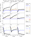 |
Fig. A.1. Global impact (thick black lines) of updated cross-sections in Li/C (top panels), Be/C (centre panels), and B/C (bottom panels) against broken-down impact per progenitor (colour-coded), as a function of rigidity. Rows show only progenitors whose relative impact is larger than 3% (resp. 2% and 1%) for Li/C (resp. Be/C and B/C); all calculations are at a fiducial Solar modulation level of 700 MV. The columns show different ways to update the cross-section sets: updating the original Galp-opt12 into OPT12 (left panels); updating the original Galp-opt22 into OPT22 (right panels), or the hybrid approach OPT12up22 (centre panels). See text for details. |
In the right panels, the reference calculation is now the original Galp-opt22 set, whereas the new calculation is based on the associated updated set OPT22. In that case, updating 56Fe reactions has a more limited impact on the flux ratios. This is consistent with the observation that the initial cross-section set Galp-opt22 was slightly overshooting the nuclear data: in Table 1, the rescaling for 56Fe (second number in the entry associated to OPT22) is, on average, close to 1 (i.e., the model prediction was already close to the data). In addition, with Fe fragmentation ranking at the ≲10% level (see Fig. 8), the combination of these last two numbers falls in the percent range at most. In this context, the most significant impact in LiBeB/C is from updating 16O fragmentation reactions.
Finally, the middle panels shows the hybrid case, where the initial parametrisation is Galp-opt12 (for all measured and unmeasured cross sections), but where we substitute for measured cross section an update of the original Galp-opt22 (so called OPT12up22 set); we recall that this was motivated by the more realistic energy dependence provided in the Galp-opt22. This configuration is expected to be the most realistic, and we see that the ratios are maximally impacted, with Li/C maximally enhanced (up to ∼40%). Moreover, these changes are now dominated by the updated Fe fragmentation.
Appendix B: Impact of recent F, Ne, Na, Mg, Al, Si, and Fe AMS-02 data
In a propagation run, while we do not fit the primary species, we rescale primary source abundances on a specific high-energy point. As illustrated in Génolini et al. (2019), this procedure is sufficient to match primary CR progenitors of LiBeB (provided we fix correctly the universal source slope). Moreover, the secondary-to-primary ratios are insensitive to this source slope (Maurin et al. 2002; Génolini et al. 2015).
In practice, to ensure the most accurate calculation, it is best to use the most-recent data available to normalise these source abundances. We use AMS-02 elemental data at 50 GV when available and HEAO3 data (Engelmann et al. 1990) at 10.6 GeV/n otherwise.
In our previous LiBeB/C analysis (Weinrich et al. 2020b), only AMS-02 data for the progenitors C, N, and O were available (Aguilar et al. 2017, 2018b). For this publication, we can rely on AMS-02 data for more progenitors, namely F, Ne, Na, Mg, Al, Si, and Fe (Aguilar et al. 2020, 2021a,b), but also C, N, and O fluxes for 7 years of data (Aguilar et al. 2021a). Figure B.1 illustrates by how much the Li/C (thick yellow dashed line), Be/C (green dashed line), and B/C (thin blue dashed line) ratios are impacted when these new data are taken into account in the calculation. We see that Li/C and Be/C are the most impacted ones, but only at a few percent level. This is understood as follows: first, N (resp. Na and Ne) contributes to the percent level (resp. negligibly) to LiBeB production (Génolini et al. 2018), so that a small discrepancy between AMS-02 and HEAO3 data would have no impact on the calculated LiBeB; second, Fe is responsible for up to tens of percent of Li, a few percent on Be, and almost no impact on B. This ordering is consistent with the one seen in Fig. B.1, and with the fact that AMS-02 data for Fe are slightly above HEAO3 ones (Aguilar et al. 2021b).
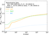 |
Fig. B.1. Impact of using the recently published AMS-02 data in the LiBeB/C calculation. The calculation relies on the use of C, N, O, F, Ne, Na, Mg, Al, Si, and Fe data from AMS-02, and HEAO-3 data for all other elements, whereas our previous analysis (Weinrich et al. 2020b), relied on C, N, O AMS-02 data (only available LiBeB progenitors from this experiment at the time) and HEAO-3 data for all other progenitors. |
CALET has recently published new data for the C, O and Fe fluxes (Adriani et al. 2020, 2021), which were found to be respectively ∼30% and ∼27% lower than the AMS-02 ones. This difference for C and O would certainly impact the production of lighter elements, but taking ratios of elements, as we do here, cancels out these yet to be explained differences.
Appendix C: Further checks on transport parameters
In the main text, we only discuss results for the SLIM propagation configuration (see Sect. 5.1). For completeness, we show in Fig. C.1 the constraints set on the transport parameters in the two other configurations QUAINT and BIG (Génolini et al. 2019); these configurations were considered in several of our previous studies (Génolini et al. 2019; Boudaud et al. 2020; Weinrich et al. 2020a,b), in particular in the context of dark matter analyses (Génolini et al. 2021; Calore et al. 2022). The respective free parameters for the three configurations are: (i) for SLIM, K0, δ, Rl, and δl, that is diffusion normalisation and slope with a low-rigidity break; (ii) for QUAINT, K0, δ, η, Va, Vc, that is diffusion without a low-rigidity break but a possible upturn in the non-relativistic regime (β replaced by βη in Eq. 2), re-acceleration, and convection; (iii) for BIG, K0, δ, Rl, and δl, Va, and Vv, that is diffusion with a low-rigidity break, reacceleration, and convection.
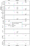 |
Fig. C.1. Same as Fig. 9, but also showing the parameter constraints for the QUAINT and BIG propagation configurations. |
As in SLIM, BIG and QUAINT show a better  /dof and
  for all the updated cross-section sets, with OPT12up22 providing the best-fit for all transport configurations. Also, moving from OPT12 to OPT12up22, and OPT22, the significance of the low-rigidity break decreases (δl consistent with zero for the latter set). However, at variance with SLIM, the parameter K0 is no longer sensitive to the production cross-section set considered, that is whether we use the original Galp-opt12 set (violet stars) or the updated ones (grey and black symbols). Actually, although Va and Vc are consistent for all the different cross-section sets, their best-fit values and 1σ upper limits are larger for the updated sets: convection and reacceleration dominate over diffusion below tens of GV (e.g. Derome et al. 2019; Vecchi et al. 2022), and the fit prefers to modify these parameters instead of adjusting K0.
All Tables
Ratio of high-energy rescaling factors between two methods tested, , with ‘fit > 1.5 GeV/n’ for which the cross-section is constant above 1.5 GeV/n (fit on existing data and their errors) and ‘no-fit’ for which the model goes through all available points.
All Figures
|
Fig. 1. Relative difference on Li/C (top), Be/C (middle), and B/C (bottom) between RFe (progenitors up to Fe, Z = 26) and RSi (progenitors up to Si, Z = 14) as a function of rigidity. The comparisons are carried out for four cross-section parametrisations available in the literature: Galp-opt22 (dotted lines), S01 (dash-dotted lines), W03 (dotted lines), and Galp-opt12 (solid lines). The enhanced production observed with Galp-opt22 motivates the re-analysis of the LiBeB production cross sections. |
| In the text | |
|
Fig. 2. Comparison of models and nuclear data for the fragmentation cross sections of 56Fe, 28Si, 24Mg, 20Ne, and 16O into Li (left), Be (centre), and B (right) isotopes and associated ghosts. The references for the data points are gathered in Fig. 5. |
| In the text | |
|
Fig. 3. Same as Fig. 2, but for 15, 14N, 12C, and 10, 11B progenitors. The references for the data points are gathered in Fig. 5. |
| In the text | |
|
Fig. 4. Same as Fig. 2, but for and 10, 9, 7Be and 7Li progenitors. The references for the data points are gathered in Fig. 5. |
| In the text | |
|
Fig. 5. References for all data points shown in Figs. 2–4, sorted from the most recent to the older ones. Specific labels from the original GALPROP files are [imos], [We96], and [NU98], which correspond to Igor Moskalenko’s additional data, Bill Webber private communication on Ramaty et al. (1997), and data retrieved from Nuclex (Ivanov et al. 1998) respectively. |
| In the text | |
|
Fig. 6. Comparison of original (Galp-opt22, thin black lines labelled ‘OLD XS’) and updated (OPT22, thick coloured lines labelled ‘NEW XS’) production cross sections, for 56Fe (left) and 16O (right) fragmenting into Be isotopes. The two branches seen in some of the updated cross sections above 1.5 GeV/n illustrate two different procedures to update them (fit of a constant or spline passing through the data, see Sect. 3.2.1). The ratio of the values in these two branches at high energy corresponds to the values |
| In the text | |
|
Fig. 7. Enhancement of Li/C (orange thick lines), Be/C (green lines), and B/C (blue thin lines) flux ratios with regard to calculations performed using Galp-opt12 (used in all recent studies). The three sets of curves correspond to the updated production cross-section sets OPT12 (dashed lines), OPT12up22 (solid lines), and OPT22 (dash-dotted lines). |
| In the text | |
|
Fig. 8. Colour-coded ranked progenitors (elements) of the Li, Be, and B (from top to bottom) fluxes as a function of rigidity. Calculations are based on OPT12up22 production cross-section set with fluxes modulated at 700 MV. For readability, only contributing fractions larger than 1% are shown. |
| In the text | |
|
Fig. 9. Best-fit transport parameters (and uncertainties) from the fit to AMS-02 LiBeB/C data using different cross-section sets: from left to right, the original Galp-opt12 set used in Génolini et al. (2019) and Weinrich et al. (2020b), and the three updated sets obtained in this paper (OPT12, OPT12up22, and OPT22). The next-to-last and last panels show the |
| In the text | |
|
Fig. 10. Best-fit and 1σ envelopes for the diffusion coefficient, Eq. (2), associated to the parameters shown in Fig. 9 and for the same cross-section sets (L = 5 kpc). For readability, we do not show the envelopes for OPT12 and OPT22 as they are similar to those for OPT12up22. |
| In the text | |
|
Fig. 11. Flux ratios (top), residuals (centre) and |
| In the text | |
|
Fig. 12. Correlation between log10(K0) and the normalisation factor |
| In the text | |
|
Fig. 13. Isotopic ratios of Li, Be, and B (from top to bottom panel) calculated from the best-fit models to AMS-02 LiBeB/C (at fixed L = 5 kpc). The production cross-section sets considered are the original Galp-opt12 (dotted lines) and the updated sets OPT12 (dashed lines), OPT12up22 (solid lines), and OPT22 (dash-dotted lines); the suffix ‘-U’ in the labels recalls that we use here unbiased cross-section sets, see Eq. (11). The data are from IMP (Garcia-Munoz et al. 1977a,b, 1981), Balloon ’73/08 (Hagen et al. 1977), Balloon ’77/05 (Buffington et al. 1978), Balloon ’77/09 (Webber & Kish 1979), Balloon ’70/06 (Bjarle et al. 1979), ISEE3 (Wiedenbeck & Greiner 1980; Mewaldt et al. 1981; Krombel & Wiedenbeck 1988), HEIST (Gibner et al. 1992), Ulysses (Connell 1998), Voyager1&2 (Lukasiak 1999), SMILI-II (Ahlen et al. 2000), ISOMAX (Hams et al. 2004), ACE (Yanasak et al. 2001; de Nolfo et al. 2006), AMS-01 (Aguilar et al. 2011), PAMELA (Menn et al. 2018; Nozzoli & Cernetti 2021). |
| In the text | |
|
Fig. A.1. Global impact (thick black lines) of updated cross-sections in Li/C (top panels), Be/C (centre panels), and B/C (bottom panels) against broken-down impact per progenitor (colour-coded), as a function of rigidity. Rows show only progenitors whose relative impact is larger than 3% (resp. 2% and 1%) for Li/C (resp. Be/C and B/C); all calculations are at a fiducial Solar modulation level of 700 MV. The columns show different ways to update the cross-section sets: updating the original Galp-opt12 into OPT12 (left panels); updating the original Galp-opt22 into OPT22 (right panels), or the hybrid approach OPT12up22 (centre panels). See text for details. |
| In the text | |
|
Fig. B.1. Impact of using the recently published AMS-02 data in the LiBeB/C calculation. The calculation relies on the use of C, N, O, F, Ne, Na, Mg, Al, Si, and Fe data from AMS-02, and HEAO-3 data for all other elements, whereas our previous analysis (Weinrich et al. 2020b), relied on C, N, O AMS-02 data (only available LiBeB progenitors from this experiment at the time) and HEAO-3 data for all other progenitors. |
| In the text | |
|
Fig. C.1. Same as Fig. 9, but also showing the parameter constraints for the QUAINT and BIG propagation configurations. |
| In the text | |
Current usage metrics show cumulative count of Article Views (full-text article views including HTML views, PDF and ePub downloads, according to the available data) and Abstracts Views on Vision4Press platform.
Data correspond to usage on the plateform after 2015. The current usage metrics is available 48-96 hours after online publication and is updated daily on week days.
Initial download of the metrics may take a while.