| Issue |
A&A
Volume 639, July 2020
|
|
|---|---|---|
| Article Number | A7 | |
| Number of page(s) | 27 | |
| Section | Stellar structure and evolution | |
| DOI | https://doi.org/10.1051/0004-6361/202037585 | |
| Published online | 01 July 2020 | |
Li-rich K giants, dust excess, and binarity⋆,⋆⋆
1
Institut d’Astronomie et d’Astrophysique, Université Libre de Bruxelles, ULB, CP 226, Boulevard du Triomphe, 1050 Brussels, Belgium
e-mail: This email address is being protected from spambots. You need JavaScript enabled to view it.
2
Instituut voor Sterrenkunde, KU Leuven, Celestijnenlaan 200D Bus 2401, 3001 Leuven, Belgium
Received:
27
January
2020
Accepted:
30
April
2020
Abstract
The origin of the Li-rich K giants is still highly debated. Here, we investigate the incidence of binarity among this family from a nine-year radial-velocity monitoring of a sample of 11 Li-rich K giants using the HERMES spectrograph attached to the 1.2 m Mercator Telescope. A sample of 13 non-Li-rich giants (8 of them being surrounded by dust according to IRAS, WISE, and ISO data) was monitored alongside. When compared to the binary frequency in a reference sample of 190 K giants (containing 17.4% of definite spectroscopic binaries – SB – and 6.3% of possible spectroscopic binaries – SB?), the binary frequency appears normal among the Li-rich giants (2/11 definite binaries plus 2 possible binaries, or 18.2% SB + 18.2% SB?), after taking account of the small sample size through the hypergeometric probability distribution. Therefore, there appears to be no causal relationship between Li enrichment and binarity. Moreover, there is no correlation between Li enrichment and the presence of circumstellar dust, and the only correlation that could be found between Li enrichment and rapid rotation is that the most Li-enriched K giants appear to be fast-rotating stars. However, among the dusty K giants, the binary frequency is much higher (4/8 definite binaries plus 1 possible binary). The remaining 3 dusty K giants suffer from a radial-velocity jitter, as is expected for the most luminous K giants, which these are.
Key words: binaries: general / stars: evolution / stars: late-type
Radial velocities are only available at the CDS via anonymous ftp to cdsarc.u-strasbg.fr (130.79.128.5) or via http://cdsarc.u-strasbg.fr/viz-bin/cat/J/A+A/639/A7
Based on observations made with the Mercator Telescope, operated on the island of La Palma by the Flemish Community, at the Spanish Observatorio del Roque de los Muchachos of the Instituto de Astrofísica de Canarias.
© ESO 2020
1. Introduction
The first Li-rich K giant was discovered by Wallerstein & Sneden (1982), rapidly followed by many others (see Bharat Kumar et al. 2018, and references therein). Recently, large surveys like Gaia-ESO, LAMOST, and GALAH further increased the number of known Li-rich K giants (Casey et al. 2016, 2019; Smiljanic et al. 2018; Singh et al. 2019; Deepak & Reddy 2019). As an illustration, the number and frequency of Li-rich stars (i.e. with log ϵ(Li) ≳ 1.5 in a scale where log ϵ(H) = 12) among G and K giants evolved from 10/644 (1.5%; Brown et al. 1989), 3/400 (0.75%; Lebzelter et al. 2012), 23/8535 (0.27%; Martell & Shetrone 2013), 15/2000 (0.75%; Kumar et al. 2011, 2015), 9/1175 (0.76%; Casey et al. 2016), 335/51982 (0.64%; Deepak & Reddy 2019) up to a record high of 2330/305793 (0.76%; Casey et al. 2019). It therefore seems that the frequency of Li-rich stars among G-K giants is about 0.7%. Li-rich giants represent a puzzle in the framework of stellar evolution since Li is predicted to disappear when the star ascends the red giant branch (RGB). This decrease in Li abundance on the RGB results from Li depletion by nuclear burning during the pre-main sequence and main sequence phases, and its subsequent dilution by the first dredge-up during the ascent of the RGB. Moreover, thermohaline mixing causes additional Li destruction at the RGB bump (Charbonnel & Lagarde 2010; Angelou et al. 2015; Lattanzio et al. 2015; Charbonnel et al. 2020). An alternative model for Li enrichment at the RGB bump was proposed by Denissenkov & Herwig (2004) and suggests that rapid rotation (due to the presence of a stellar companion and the resulting tidal locking) could trigger extra-mixing leading to Li production. Casey et al. (2019) put forward the same scenario without restricting its operation solely to the RGB bump.
As a result, starting from the present interstellar-medium abundance of log ϵ(Li) = 3.3, the Li abundance after the first dredge-up is expected to be lower than about 1.5 to 1.8 in Population I K giants. However, some K giants do not conform to these predictions, and some of these Li-rich K giants have Li abundances that are even larger than the present interstellar-medium value (e.g. da Silva et al. 1995; de La Reza & da Silva 1995; de La Reza et al. 1996; Balachandran et al. 2000; Ruchti et al. 2011; Casey et al. 2016; Takeda & Tajitsu 2017; Bharat Kumar et al. 2018).
A number of K giants also exhibit rapid rotation rates that some authors (e.g. De Medeiros et al. 1996, 2000; Drake et al. 2002; Carlberg et al. 2012; Smiljanic et al. 2018; Charbonnel et al. 2020) claimed to be correlated with high lithium abundances. This is especially well illustrated by Fig. 3 of De Medeiros et al. (2000) which reveals that among 20 Li-rich stars (log ϵ(Li) ≥ 2.0), 15 are rapid rotators (Vrot sin i ≥ 5 km s−1). The situation is even more extreme for the 14 stars with log ϵ(Li) ≥ 2.5, among which 12 are rapid rotators.
At about the same time, K giants with IR excesses were reported (Zuckerman et al. 1995; Plets et al. 1997), based on data from the Infrared Astronomy Satellite (IRAS; Neugebauer et al. 1984), which surveyed the sky at 12, 25, 60, and 100 μm. Infrared excess is not expected in giant stars prior to the late asymptotic giant branch (AGB) phase. Gregorio-Hetem et al. (1993), de la Reza et al. (1997), Castilho et al. (1998), Fekel & Watson (1998), Jasniewicz et al. (1999), Reddy et al. (2002), and Reddy & Lambert (2005) suggested that several of the Li-rich K giants are surrounded by dust shells as they exhibit IR excesses, sometimes starting at 12 μm and sometimes at much longer wavelengths (60 μm). These early studies were based on IRAS data.
Various hypotheses have been proposed to explain the combination of high Li abundances, rapid rotation rates, and IR excesses, including the accretion of giant planets (e.g. Siess & Livio 1999; Casey et al. 2016), or a sudden transport of matter that could eject a dusty shell (de la Reza et al. 2015). In both cases, based on dust shell evolutionary models, the IR excess and a large amount of Li in RGB stars should be transient phenomena that would last for a few 104 years. Observations suggest that, if dust shell production is a common by-product of Li enrichment mechanisms, the IR excess stage should be very short-lived (Rebull et al. 2015; de la Reza et al. 2015). Indeed, even the early studies investigating the possible correlation between large Li abundances and dust excesses did not deliver strong evidence on a purely statistical basis. For instance, Fekel & Watson (1998) found 6 giants with greater-than-typical lithium abundances out of 39 giants with IR excess, which they point out is similar to the fraction of stars with enhanced Li found in normal field giants. Jasniewicz et al. (1999) identified 8 Li-rich stars out of 29 stars with IR excesses, but no correlation between Li abundance and IR excess. Lebzelter et al. (2012) report on 3 Li-rich giants (out of more than 400 studied), none of which have IR excesses suggestive of mass loss.
The spatial resolution of IRAS was relatively low (a few arcminutes), making the identification of the optical counterpart difficult, especially in regions with high source density or high background due to the so-called IR cirruses (Jura 1999). Background galaxies with a large amount of interstellar material (like hyperluminous IR galaxies; Rowan-Robinson 2000) could also be responsible for an apparent IR excess if they happen to lie along the same line of sight as the target star (see for instance the case of HD 24124 described by Kim et al. 2001).
To clear these ambiguities, the reality of the IR excesses around (Li-rich) K giants was later re-examined (Kim et al. 2001; Kumar et al. 2015; Rebull et al. 2015) with much better quality data from either the Infrared Space Observatory (ISO; Kessler et al. 1996) or the Wide-field Infrared Survey Explorer (WISE) spacecraft, delivering four IR magnitudes (at 3.35, 4.6, 11.6, and 21.1 μm; Wright et al. 2010; Cutri et al. 2013) at a higher spatial resolution and with a better sensitivity than IRAS. The correlation between Li richness and dust excess remained weak, at least for these comparatively short IR bands. Kumar et al. (2015) for instance report on a search for IR excesses (combining WISE and IRAS data) in 2000 K-type giants. None of the far-IR excess sources studied by these latter authors are lithium-rich, and of the 40 Li-rich sources, only seven show IR excess. Rebull et al. (2015) performed a similar study and conclude that, intriguingly, the largest IR excesses all appear in Li-rich K giants, though very few Li-rich K giants have IR excesses (large or small). According to Rebull et al. (2015), these largest IR excesses also tend to be found in the fastest rotators, and there is no correlation of IR excess with the carbon isotopic ratio 12C/13C.
Since fast rotation in Li-rich giants could be caused by either planet ingestion or synchronisation within a binary system, a search for either stellar or planetary companions around these giants would be worthwhile. Similarly, a link between dust excess and binarity has been established very convincingly for post-AGB (Van Winckel 2003) and post-RGB (Kamath et al. 2016) stars. It would therefore be of interest to check whether this correlation also holds for K giants with a dust excess. Strangely enough, there has been no convincing estimate so far of either the binary frequency among Li-rich K giants or among dusty K giants, since the studies of Ruchti et al. (2011) and Fekel & Watson (1998), respectively, relied on very scarce data. De Medeiros et al. (1996) claimed that their CORAVEL monitoring of Li-rich giants did not reveal any abnormal frequency of binaries, but they did not substantiate their claim by publishing the individual radial velocities (RVs).
In the present study, we therefore aim to check whether or not dust-rich K giants and Li-rich K giants have a higher-than-normal binary frequency. The paper is organised as follows. The studied samples are described in Sect. 2, along with the main properties of their stellar members (spectral energy distribution (SED) and location in the Hertzsprung–Russell (HR) diagram). The RV monitoring is presented in Sect. 3. Orbital elements and the binary frequency are presented in Sects. 4 and 5, respectively, and conclusions are drawn in Sect. 6.
2. The stellar samples and their properties
2.1. Sample synopsis
Three samples are considered in this paper. A small sample of 11 Li-rich and 13 non-Li-rich K giants (hereafter sample S1) extracted from Charbonnel & Balachandran (2000) and Kumar et al. (2011) is described in Sect. 2.2 (Tables 1 and 2). The RVs for these stars were extensively monitored with the HERMES spectrograph (Raskin et al. 2011) for 10 years, starting in April 2009 (Sect. 3). Sample S1, which can also be divided into 8 dusty and 16 non-dusty K giants, served to test the possible correlation between binarity and IR excess due to dust.
Stellar sample S1.
Fundamental parameters of the S1 stars.
A second, more extended sample of 56 Li-rich giants (hereafter sample S2) was collected from the work of Bharat Kumar et al. (2015) and Charbonnel et al. (2020) to infer the binary frequency from the Gaia DR2 RV standard deviations (Sect. 5.1). Seven stars have been excluded from the samples of these latter authors because they have no RV available in Gaia DR2 (namely HD 35410, HD 71129, HD 86634, HD 138289, HD 138905, HD 183912, and HD 188114). There are 8 stars in common between samples S1 and S2. The properties of this sample are presented in Sect. 5.4 and Table A.1.
Finally, sample R contains 190 K giants selected from the Kepler data set (Sect. 2.3) and monitored with the HERMES spectrograph since April 2016 (Table A.2). Here, it serves as a reference sample against which the binary frequency of sample S1 can be compared.
2.2. HERMES sample S1
2.2.1. Selection and spectral energy distributions
The sample of 11 Li-rich giants was selected from the list of Charbonnel & Balachandran (2000), with two additions from Kumar et al. (2011), HD 63798 and HD 90633. These Li-rich stars are listed in the first part of Table 1, and are a mixture of stars on the RGB (some close to the bump), in the red clump and along the early AGB (as shown in Sect. 2.2.3). In this sample, HD 112127 has sometimes been classified as a carbon star of type R (Barnbaum et al. 1996). Table 1 also provides a proxy for the rotational velocity Vrot sin i. It is equal to  , where σCCF is the width of a Gaussian fitted to the cross-correlation function used to derive the RV (Sect. 3), and σ0 = 3.5 km s−1 is the instrumental width corresponding to the resolution of 86 000 for the HERMES spectrograph (Raskin et al. 2011). There is a clear tendency for the most Li-enriched K giants to be the fastest rotating stars, as already pointed out by Drake et al. (2002) and Smiljanic et al. (2018).
On top of the Li-rich K giants, we selected 13 stars from the list of K giants with suspected IR excesses (as initially inferred from the IRAS data) from Fekel & Watson (1998), itself being a subsample of Zuckerman et al. (1995), who list the corresponding IRAS fluxes (their Table 1). These K giants with a suspected IR excess are listed in the second part of Table 1. Because an IR excess has in the end not been confirmed for all of them, this second part of the sample is denoted by “non-Li-rich stars”, so as to avoid any ambiguity in the terminology.
Given the difficulties in establishing firm IR excesses using IRAS data alone (as explained in Sect. 1), we sought confirmation from other IR data, namely WISE, AKARI (Murakami et al. 2007) and ISO (Kim et al. 2001). To this end, we built the spectral energy distributions (SEDs) using the tool described by Escorza et al. (2017) to retrieve broadband photometry from Simbad, and find the extinction on the line of sight (see more on this below). The IRAS fluxes listed as upper limits were removed from the SED, but the reality of any dust excess in cases like HD 119853 (Fig. B.3) or HD 156115 (Fig. B.5) with just one (firm, i.e. non-upper limit) IRAS band (marginally) deviating from the MARCS model would still be questionable were it not confirmed by the ISO data of Kim et al. (2001). For the sake of concision, Figs. B.1−B.8 present only those SEDs exhibiting a confirmed IR excess, whereas Fig. B.9 presents one SED without IR excess for comparison (HD 6). These plots show the best-fitting reddened MARCS model (red curves; Gustafsson et al. 2008) on top of the observed photometry, while the unreddened MARCS model is displayed in black. Since the fitting process is ill-behaved (because of a strong coupling between the effective temperature Teff and the reddening EB − V), it was necessary to obtain a first guess of Teff from the literature and listed in Table 2 (a more detailed description of the contents of this table is given in Sect. 2.2.3). Moreover, fixing the gravity log g also helped to obtain reasonable fits. A first estimate of the gravity was obtained from the location of the star in the HR diagram (see Sect. 2.2.3), before applying the de-reddening correction.
This way, a satisfactory SED fit could be obtained, often with the minimum possible reddening (listed as well in Table 2), and with a de-reddened (V − K)0 colour temperature (derived from the reddening; Cardelli et al. 1989; Bessel et al. 1998) in good agreement with the literature Teff value. An exception is the star HD 212320 (HIP 110532) whose de-reddened (V − K)0 index of 1.55 yields an uncomfortably warm temperature of 5660 K, as compared to literature estimates of 5030 K (Hekker & Meléndez 2007) or 4825 K (Stock et al. 2018). Therefore, in the remainder of this paper, we adopt for HD 212320 the non-dereddened colour temperature of 5080 K, in better agreement with the spectroscopic temperatures.
Those stars with a confirmed IR excess are listed in bold face in Table 1. We see that, among our sample of Li-rich giants, only two are simultaneously dust-rich (HD 30834 and HDE 233517).
2.2.2. Origin of the dust excess observed in sample S1
The IR excess observed in the dusty K giants is peculiar in that it involves very cool dust (Tdust < 100 K according to the model of Jura 1999, and Kim et al. 2001); the excess is often restricted to wavelengths longwards of 60 μm. Except for HDE 233517, where the IR excess starts at 10 μm (Fig. B.8), dusty K giants strongly differ from mass-losing AGB stars where dust features are seen from 10 μm onwards (Waters et al. 1999). When mass loss stops, their dust-emission peak progressively moves towards longer wavelengths as the dust shell becomes detached and cools down. In non-binary post-AGB stars with an expanding dust shell, IR excesses may start from close to 10 μm up to about 20 μm (Van Winckel 2003; Gezer et al. 2015). When the star becomes surrounded by a (proto-)planetary nebula (PPN or PN), dust emission peaks around 30 μm (e.g. PPN SAO 34504 and PN NGC 7027, where dust emission peaks at 30 and 33 μm, respectively; Waters et al. 1999). For dusty K giants, where the dust emission peaks longwards of 60 μm, the dust shell is detached, indicating that the mass-loss process is no longer active. The dust temperatures derived by Kim et al. (2001) from their ISO data and based on the hypothesis of a detached shell are listed in Table 1.
For HDE 233517, the large inferred dust mass has been suggested to be either the result of the disintegration of comets (Jura 1999; Fisher et al. 2003) or of the ingestion of a large planetary body or low-mass star (Jura 2003). The presence of warm dust and of a flared disk inferred by Jura (2003) is reminiscent of the situation prevailing among binary post-AGB stars (Kluska et al. 2019). Although our HERMES data do not flag HDE 233517 as a binary system, Gaia DR2 data suggest the opposite (see Sect. 5).
2.2.3. Dusty and Li-rich K giants of sample S1 in the Hertzsprung-Russell diagram
The HR diagram of the S1 stars was constructed in the following way. First, the colour temperature was computed from the de-reddenned V − K index (with V and K taken from the Simbad database) using the Bessel et al. (1998) calibration (relation “abcd” in their Table 7). The colour excess EB − V used to de-redden the V − K index is the one obtained from the SED fit (Table 2), and the EV − K/EB − V ratio was taken from Cardelli et al. (1989). The de-reddening correction (including both circumstellar and interstellar contributions) was computed only for those stars showing the presence of circumstellar dust. For the other stars, no interstellar de-reddening correction was applied since the stars are relatively nearby (closer than 350 pc, except for HDE 233517, for which the colour excess has been derived), meaning that the interstellar reddening is considered negligible. The bolometric correction for the K band has been taken from Bessel et al. (1998) for oxygen-rich stars, and from Kerschbaum et al. (2010) for the carbon star HD 112127 (their Eq. (1)). The luminosity is then derived from the bolometric magnitude combined with the Gaia DR2 parallax (Gaia Collaboration 2018). There is no need to use Bayesian estimates for the distance because all the targets stars are close enough for the ratio ϖ/σϖ to be sufficiently large (≥19) to avoid biasing the distance when inverting the parallax.
For the sake of homogeneity, the temperature used to construct the HR diagram is the colour temperature, except for HD 212320 (for the reason discussed in Sect. 2.2.1) where Teff is taken instead from Hekker & Meléndez (2007).
Before discussing the HR diagram thus constructed (Fig. 1), we first compare in Table 3 the stellar parameters listed in Table 2 with their Bayesian estimates provided by Stock et al. (2018) for the three stars in common between the two samples, namely HD 27497 (=HIP 20268), HD 116292 (=HIP 65301) and HD 212320 (=HIP 110532). The luminosities are in good agreement, and the temperatures as well (except for HD 212320).
 |
Fig. 1. Li-rich (large filled dots) and dust-rich (open squares) K giants from sample S1 in the HR diagram. Small filled dots are non-Li-rich K giants. Green symbols denote SB, as discussed in Sect. 5. Small red dots indicate the presence of regular small-amplitude variations, whereas large crosses indicate irregular small-amplitude variations (RV jitter). STAREVOL tracks (Siess et al. 2000; Siess & Arnould 2008) are labelled according to their initial mass, and correspond to solar metallicity. Tracks evolving along the core He-burning phase are depicted in blue, whereas tracks along the AGB are displayed in red. The red clump as defined by Deepak & Reddy (2019; their Fig. 1) is represented by the dashed rectangle. The bump is well visible on the 1 M⊙ track as the hook feature located to the lower right of the red clump region. |
Comparison between the stellar parameters derived in this study (Table 2) with their Bayesian estimates from Stock et al. (2018).
Evolutionary tracks for stars of solar metallicity (given the small metallicity range of our target stars as revealed by Table 2) from the STAREVOL code (Siess et al. 2000; Siess & Arnould 2008) are displayed as well in Fig. 1.
Some Li-rich K giants are located in the red clump (dashed rectangle in Fig. 1), but several are also spread along the giant branch (either RGB or E-AGB), namely HD 787, HD 9746, HD 30834, HD 39853, and HD 233517. The HR diagram of Fig. 1 is similar to that of Charbonnel & Balachandran (2000) with its extension along the giant branch, and both contrast with the well-documented claim (based on asteroseismologic data) by Singh et al. (2019) that all Li-rich stars are restricted to the red clump. Nevertheless, Casey et al. (2019) and Deepak & Reddy (2019) disagree with that claim, quoting a frequency of 75−85% Li-rich stars located in the red clump (not 100%). The reason for this difference between Singh et al. (2019) and all other studies most likely resides in the fact that Singh et al. (2019) restricted their study to super-Li-rich stars with log ϵ(Li) ≥ 3.0. As confirmed by all the other studies quoted above (see especially Fig. 3b of Deepak & Reddy 2019), super-Li-rich stars are largely confined to the red clump. This leaves room then for a limited fraction of Li-rich stars (of the order of 15−25%) that may still be found along the RGB.
2.3. Reference sample R
To evaluate whether or not the binary frequencies in our dusty and Li-rich samples of K giants are peculiar, it is necessary to first evaluate this frequency in a reference sample observed as well with the HERMES spectrograph. This reference sample (listed in Table A.2; the full content of this table will be described in Sect. 5.1) contains the 160 brightest K giants (i.e. with V magnitudes in the range 8.6−11.4) observed with the Kepler satellite (Koch et al. 2010), and with known evolutionary status (from Mosser et al. 2014), along with 30 K giants from the CoRoT1 (Baglin et al. 2006) sample. Figure 2 presents the number of HERMES observations versus time-span for this reference sample of Kepler/CoRoT giants (referred to as “sample R” below). The RV observations cover the period from April 2016 to August 2019. The original purpose of this HERMES observing program is to compare the evolutionary properties of K giants with their orbital properties. The sample will be fully described in a forthcoming paper especially devoted to that issue (Jorissen et al., in prep.). Here, we simply perform a first evaluation of the binary frequency (Sect. 5.5) in sample R along the guidelines described in Sect. 5.1.
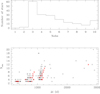 |
Fig. 2. Top panel: distribution of the number of observations per star in sample R. Bottom panel: number of HERMES observations vs. time span of the RV observations for the comparison sample of Kepler/CoRoT giants (sample R; open squares). Most of the stars have three observations spanning 300 to 900 d. Red crosses correspond to the re-sampled data of sample S1 (denoted ‘sample S1’) with Nobs and Δt modified to mimic the distribution of sample R (see Sect. 5.5). |
3. Radial-velocity observations
The RV monitoring of samples S1 and R was performed with the HERMES spectrograph attached to the 1.2 m Mercator Telescope from the KU Leuven installed at the Roque de los Muchachos Observatory (La Palma, Spain). The spectrograph is fully described in Raskin et al. (2011). The fibre-fed HERMES spectrograph is designed to be optimised both in stability as well as in efficiency, and samples the whole optical range from 380 to 900 nm in one shot, with a spectral resolution of about 86 000 for the high-resolution science fibre. This fibre has a 2.5 arcsec aperture on the sky and the high resolution is reached by mimicking a narrow slit using a two-sliced image slicer. The RV is measured by cross-correlating the observed spectrum with a spectral mask constructed on an Arcturus spectrum (e.g. Jorissen et al. 2016a). The HERMES/Mercator combination is precious because it guarantees regular telescope time. This is needed for our monitoring programme and the operational agreement reached by all consortium partners (KU Leuven, Université libre de Bruxelles, Royal Observatory of Belgium, Landessternwarnte Tautenburg) is optimised to allow efficient long-term monitoring, which is mandatory for this programme. On average, 250 nights per year are available for the monitoring (spread equally on HERMES-consortium time, and on KU Leuven time), and the observation sampling is adapted to the known variation timescale. During these nights, about 300 target stars are monitored, addressing several science cases (Gorlova et al. 2013) and delivering significant results concerning different families of long-period binaries such as Ba and CH stars (e.g. Jorissen et al. 2016a, 2019; Escorza et al. 2019), post-AGB binaries (e.g. Manick et al. 2017; Oomen et al. 2018), or sub-dwarf B stars (e.g. Vos et al. 2015). Most importantly, the long-term stability of the RVs has been assessed from the monitoring of RV standard stars from the list of Udry et al. (1999). From this sample of RV standard stars, the long-term velocity stability is estimated as 55 m s−1 (see Jorissen et al. 2016a, for details; also Sect. 5.1).
The RV monitoring of sample S1 began in April 2009, with the regular science operations of HERMES. The individual RVs are only available online at the CDS, Strasbourg. The RV curves for all target stars are presented in Figs. C.1–C.18. Some clearly allow an orbit to be computed, as done in Sect. 4.
4. Orbital elements
The available orbital solutions in sample S1 are displayed in Figs. D.2–D.8, and the orbital elements are listed in Table 4. Notes about individual stars are listed in Appendix D.
Orbital elements.
The dispersions of the O − C residuals are listed in Table 5, and they are all compatible with the HERMES accuracy, except for HD 156115, for which they amount to 0.38 km s−1. A look at Fig. D.7 reveals that the large residuals are caused by an oscillation superimposed on the long-term orbit. A similar behaviour is observed for HD 787 as well (Fig. D.2), even though it is not apparent in the value of the O − C dispersion (Table 5). The resulting orbital solutions for the HD 787 and HD 156115 residuals are listed in Table 4b under the heading Aa+Ab to distinguish them from the main AB orbit. The ratio of the outer to inner periods is 8.3 and 7.6 for HD 787 and HD 156115, respectively. These ratios are compatible in principle with the usual requirement for orbital stability in a hierarchical triple system (e.g. Tokovinin 2014). The inner periods are of the order of 1.5 years. For these small-amplitude variations to be due to orbital motion would require a (brown dwarf) companion with a mass larger than 0.015 M⊙ in the case of HD 156115 (adopting a mass of 1 M⊙ for component A according to its location in the HR diagram; see Fig. 1). The companion could be even less massive in the case of HD 787 (≥0.005 M⊙ adopting a mass of 2.5 M⊙ for component A), but the mass function is not well constrained (Table 4b). The dispersion of the O − C residuals for the Aa+Ab orbit of HD 156115 amounts to 0.26 km s−1, indicating that the Keplerian solution is not of excellent quality, since that dispersion could not be lowered to values typical of the HERMES accuracy. For HD 787, the O − C dispersion is 64 m s−1.
Binary properties of sample S1 ordered by increasing RV standard deviation σj(RV).
Similarly small-amplitude variations are also found in HD 39853 (Table 4b), and a circular Keplerian orbit with a semi-amplitude of 0.2 km s−1 could match them. As listed in Table 4, the current data do not allow us to rule out one of two possible periods (106 or 282 d).
We stress that, although not found for all long-period binary giants (see for example HD 3627, Fig. D.3), the short-term oscillations reported above are found in many of them. They were reported as well in the K giants HE 0017+0055 (Jorissen et al. 2016b), HE 1120−2122 and HD 76396 (Jorissen et al. 2016a), and HD 175370 (Hrudková et al. 2017). Except for the latter star, there was no compelling evidence to reject the possibility that the small-amplitude, approximately one-year RV oscillations could be caused by stellar pulsation2. This hypothesis gains further support from the fact that all three stars in our sample which show such small-amplitude variations (namely HD 787, HD 39853, and HD 156115) are among the most luminous stars in our sample, with log L/L⊙ > 2.5 (small red dots in Fig. 1). Incidentally, the other stars at similarly large luminosities but not showing regular, short-amplitude variations exhibit instead irregular RV jitter, another signature of envelope instability (blue crosses in Fig. 1).
5. Binary frequency
5.1. Methodology
The binary frequency has been derived by combining different strategies depending on the considered sample: (i) from the HERMES data alone (samples S1 and R), (ii) by combining HERMES with Gaia DR2 data (samples S1 and R), (iii) by combining HERMES data with other data from the literature (sample S1; Fekel & Watson 1998; Famaey et al. 2005; Gontcharov 2006), and finally (iv) from Gaia DR2 RV data (samples S1, S2, and R).
We explain each of these methods in turn in the remainder of this section. Method (i) is simply based on the evaluation of the F2 statistic. This statistic has been defined by Wilson & Hilferty (1931) as a way to approximate the reduced χ2 statistic by a reduced normal distribution 𝒩(0, 1) (of mean zero and standard deviation unity), thus making it independent from the number of degrees of freedom νj:
 (1)
(1)
where index j runs over the M different stars (1 ≤ j ≤ M) and
 (2)
(2)
where index i runs over the Nobsj RV observations RVi, j of star j. There is only one constraint (the average velocity  ) among the Nobsj variables RVi, j, and therefore νj = Nobsj − 1. In the above expressions, ϵ (the same for all HERMES observations) is the long-term stability of the spectrograph. As stated in Sect. 3, the long-term RV standard deviation of a sample of RV standard stars amounts to 0.055 km s−1 (Jorissen et al. 2016a), which would be the natural choice for ϵ. However, adopting that value in Eq. (2) would not make the F2 distribution (derived from Eq. (1)) of the reference sample R compatible with a reduced normal distribution 𝒩(0, 1) as it should after removing the binaries, defined as those stars with F2 ≥ 3.0 (this threshold is similar to the usual “3σ” cut-off, since by construction F2 behaves similarly to a reduced normal distribution). We therefore proceeded by trial and error to find the proper ϵ value ensuring that the F2 distribution behaves as a reduced normal distribution 𝒩(0, 1). Figure 3 reveals that 0.070 km s−1 is required3 to ensure the best match between a 𝒩(0, 1) distribution (blue dashed line) and the binary-free observed distribution (red curve). The same ϵ value was adopted for sample S1 (Fig. 4). However, because of the smaller sample size, the resulting F2 distribution does not match the expected 𝒩(0, 1) distribution as accurately as it does for the Kepler reference sample R of Fig. 3.
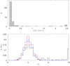 |
Fig. 3. Top panel: distribution of HERMES σj(RV) per star j of the reference sample (R) of CoRoT/Kepler K giants. Bottom: F2j distribution for the same sample. In black is drawn the full sample, and in red the sample with binaries removed (F2 ≥ 3.0), which leads to an almost perfect match between the binary-free observed F2 distribution (red curve) and the expected 𝒩(0, 1) normal-reduced distribution (blue curve). |
The problem with this method based on the F2 distribution is that it does not distinguish RV variations associated with orbital motion from variations associated with RV jitter in K giants. Thus, stars flagged as having a probability of unity of being RV variables are not necessarily spectroscopic binaries. Therefore, a visual inspection of the RV data is necessary to identify those RV variables where no obvious evidence of orbital motion is present. Those are flagged as “jitter” in Table 5 for sample S1. This RV jitter has been reported by for example Mayor et al. (1984), Carney et al. (2003), and Hekker et al. (2008) to increase with luminosity. This is also the case in sample S1, as revealed by Fig. 1 where stars with RV jitter are identified with crosses. These stars are indeed restricted to the highest luminosities in the HR diagram, as confirmed from Fig. 5.
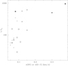 |
Fig. 5. Radial-velocity standard deviation (σ(RV), or σ(O−C) in case of orbital SBs) vs. luminosity for sample S1. Symbols are as follows: filled squares show stars with small-amplitude variations, large open circles signify SBs, crosses represent stars showing jitter, open squares show stars with no special features. We note that the jitter stars and those with small-amplitude RV variations are among the most luminous ones, as expected. |
Visual inspection of the RV curve also revealed that a drift seems to be present in the RV data of some of the S1 stars (like HD 119853; Fig. C.15). To set this visual feeling on objective grounds, methods (ii) and (iii) were used, that is, comparing the HERMES average velocity for a given target with other data sets, most often the Famaey et al. (2005) or the Gaia DR2 RV sets. Since the former covers epochs not overlapping with the time-span of the HERMES observations, any long-term drift will be easily detected as an offset between the two data sets. However, merging different RV sets requires careful a priori evaluation of possible zero-point offsets between them. The HERMES data set has been tied to the IAU system thanks to the use of Udry et al. (1999) RV standard stars. The Famaey et al. (2005) data set, which uses CORAVEL velocities (Baranne et al. 1979), is also tied to the IAU system, as checked by Gontcharov (2006; see his Tables 2 and 3). Therefore, there should be no offset between the HERMES and Famaey et al. (2005) RV sets, meaning that the latter may be used to detect long-term trends. Table 5 (for sample S1) lists the average velocity and its associated error  for the Famaey et al. (2005) RVs whenever available.
De Medeiros & Mayor (1999) also studied several stars that are in common with our sample. Nevertheless, we have not used any of the results found by these latter authors in our study, because (i) their study relies on older CORAVEL measurements that were not yet tied to the IAU system (and indeed there appears to be an offset between the HERMES system and this old CORAVEL system, which we did not try to correct at the required accuracy level; see also Sect. 2.1 and Fig. 1 of Escorza et al. 2019), and (ii) they do not add any new information.
Similarly, the offset between the average HERMES and Gaia DR2 velocities has been computed and is listed in Table 5 as  . However, this offset should first be compared to the uncertainty on
  before being used to identify a velocity drift. This uncertainty ϵ(RVG) was computed in the following manner. Figure 3 of Katz & Brown (2017) presents the expected accuracy of the average Gaia RV as a function of the number of transits used to compute it, and the stellar magnitude GRVS in the Radial Velocity Spectrometer pass band. For sample S1, an average of eight RV transits were used to derive RVG. Therefore, the corresponding curve has been approximated by a Lagrange polynomial of degree 5 in GRVS, as follows:
 (3)
(3)
For sample R, the GRVS magnitude was computed from the Gaia G magnitude using the G − GRVS calibration from Table 2 of Jordi (2018), namely
 (4)
(4)
with the r − i index derived from the Sloan Digital Sky Survey Data Release 12 (Alam et al. 2015). For sample S1, the GRVS magnitude was computed from the Gaia G magnitude using a slightly different G − GRVS calibration from Table 2 of Jordi (2018), namely
 (5)
(5)
with the Johnson – Cousins V − I index derived from the HIPPARCOS catalogue (ESA 1997). If neither V − I nor r − i were available, the typical value G − GRVS = 1 was used instead. A drift was considered as very likely when the  offset was found to be at least twice larger than the uncertainty ϵ(RVG). These situations are outlined in bold face in Tables A.2 and 5 corresponding to samples R and S1, respectively. All the other targets have
  km s−1 (already discussed by Jorissen et al. 2019), with the exception of HD 112127 where it amounts to 0.41 km s−1. Table 5 provides as well the average velocity
  of the Famaey et al. (2005) data set, and again any offset
  is outlined in boldface.
The above estimate of ϵ(RVG) is also used in method (iii) to flag binarity when the Gaia DR2 RV standard deviation (in column  ) is at least twice larger than ϵ(RVG). As above for method (ii), these values are outlined in bold face in Tables A.2 and 5.
Coming back to method (ii), that is, detecting binarity from the offset between HERMES  and Gaia DR2
  , we stress that the efficiency of this method is largely dependent upon the period and amplitude of the binary system and upon the HERMES and Gaia DR2 respective time spans. Gaia DR2 measurements span from 25 July 2014 to 23 May 2016 (56 864 ≤ (JD − 2 400 000)≤57 532, corresponding to 662 d). For sample R, Gaia DR2 and HERMES time ranges are disjointed as the HERMES observations started in May 2016 (JD 2 457 509) and the current data set extends up to August 2019 (JD 2 458 727). This situation is the most favourable to detect a RV drift between the two data sets which come in succession. A long-period binary will be detected if it causes an offset between the average Gaia DR2 and HERMES velocities that exceeds 2 × 0.3 km s−1.
For sample S1, the situation is not as clear cut because the HERMES S1 time-span (April 2009−August 2019) encompasses the Gaia DR2 epochs. Hence, the possible offset between their respective average RVs will strongly depend on their time sampling and their distribution over the orbital cycle. It is therefore impossible to make definite predictions in this case.
In summary, to flag a star as binary, either a satisfactory orbit is computable, or at least two of the following criteria must be satisfied:
-
(i)
The probability that the star has a variable (HERMES) RV is strictly larger than 0.99;
-
(ii)
a drift is seen in the HERMES data, and is confirmed by a significant offset
 , or
, or  ;
; -
(iii)
the standard deviation of the Gaia DR2 RV is larger than 2 ϵ(RVG).
Regarding criterion (iii), which was the only one available to detect binaries in sample S2, its efficiency has been evaluated by Jorissen (2019). Although that diagnostic offers a good detection efficiency for systems with orbital periods up to 1000 d (Fig. 6 of Jorissen 2019), its efficiency decreases for longer-period binaries.
Based on the extensive data available for stars of sample S1, we present in Table 5 (in column labelled SB) our final diagnostic regarding the single or binary nature of the S1 targets, and in Table A.2 we do the same for the targets of sample R. Section 5.2 presents additional comments on some S1 targets.
We defer the evaluation of the binary frequencies in these two samples to Sect. 5.3, and the discussion as to whether or not the binary frequencies among Li-rich and dusty K giants are compatible with that in the reference sample R to Sect. 5.5.
5.2. Comments on individual stars in sample S1
Not mentioned in Table 5 are the RV data from Fekel & Watson (1998) which confirm the absence of any long-term drift for HD 6, HD 153687, and HD 221776 – and thus their non-binary nature. HD 153687 and HD 221776 are nevertheless flagged as RV variables by the F2 criterion, but a look at their RV curves (Figs. C.16 and C.17) reveals no orbital signature. These stars are therefore flagged as “RV jitter”. Similar RV jitter is observed for HD 9746 and HD 30834 (Figs. C.3 and C.4), and it is noteworthy that all four jitter stars have their F2 values just above the threshold value flagging them as RV variables (F2 around 4 for HD 9746, HD 30834 and HD 153687, and 12 for HD 221776). These F2 values nevertheless remain much smaller than those of the genuine SB (F2 in excess of 25). Fekel & Watson (1998) also report scattered velocities for HD 30834 (−16.7, −17.1, −17.2, and −17.6 km s−1, as compared to −17.1 ± 0.1 km s−1 from HERMES).
HD 34043 has a F2 of 3.27 and a probability of 0.99 of having a variable RV. Although not formally flagged as a RV variable, HD 34043 is very close to the adopted threshold, and may be considered as a further case of RV jitter (Fig. C.5).
With σ(RV) = 0.30 km s−1 and F2 = 25.5, HD 39853 is formally flagged as RV variable from the HERMES data; however, its RV curve does not reveal any clear long-term drift (top panel of Fig. C.6). The Pulkovo catalogue provides a velocity of 81.3 ± 0.4 km s−1 as compared to 81.6 ± 0.3 km s−1 for HERMES, confirming the absence of large-amplitude variations. However, a periodogram analysis based on the phase-dispersion-minimisation method of Stellingwerf (1978) (Fig. C.7) reveals the existence of a periodic signal of small amplitude (K ∼ 0.2 km s−1), with a period that could either be 106 or 282 d, and with zero eccentricity (the 282 d signal is represented on the upper panel of Fig. C.7). This would imply very small mass functions of either 8.8 × 10⁻⁸ M⊙ (for the 106 d period) or 1.7 × 10⁻⁷ M⊙ (for the 282 d period). If these variations were indeed associated to a Keplerian motion (rather than to envelope pulsations), they would correspond to a companion of 6 to 7 Jupiter masses (assuming a stellar mass of 1.5 M⊙ and an orbit seen edge-on).
The HERMES data reveal a long-term drift for HD 119853 (Fig. C.15) and therefore this star should be included in the category of possible binaries (labelled “SB?”). This conclusion is supported by the velocity listed in the Pulkovo catalogue (−9.7 ± 0.8 km s−1; Gontcharov 2006), 1σ away from the HERMES average velocity (−8.67 km s−1). The velocities (−10.2 and −8.7 km s−1) measured by Fekel & Watson (1998) also support the hypothesis that HD 119853 is a binary system.
Hints that HD 43827 (Fig. C.9) could have a variable velocity are provided by the Pulkovo catalogue (−6.5 ± 0.8 km s−1 as compared to −8.0 km s−1 from HERMES and to −8.2 and −8.5 km s−1 from Fekel & Watson 1998). However, since these variations could also be caused by an intrinsic RV jitter, as for the other stars discussed above, HD 43827 is not included in our list of binaries, especially since the HERMES velocities alone are characterised by a small standard deviation of 0.08 km s−1.
HD 233517 is special in sample S1 since it is the only star for which the two binary criteria involving Gaia DR2 data are positive (and may thus be flagged as a binary according to the criteria described in Sect. 5.1), whereas the HERMES F2 criterion is not met, although it is not missed by a significant margin, as F2 = 0.99. Given the very specific SED of that star (Fig. B.8), reminiscent of dusty post-AGB systems surrounded by a circumbinary disc (Sect. 2.2), this binary classification is not surprising.
5.3. Binary frequency in samples R and S1
In samples R and S1, there are 33/190 (17.4%) and 8/24 (33.3%) stars, respectively, satisfying the conditions of Sect. 5.1 for definite SBs, as summarised on line “Total (S1)” in Table 6. We slightly relaxed the above criteria to define possible SBs when just one of the above conditions (i)−(iii) is satisfied. For sample R, this yields 12/190 (or 6.3%) supplementary “SB?”. For sample S1, this yields 8/24 stars, from which we nevertheless exclude 4 stars which we flag as “jitter”, a category made possible by the large number of data points that do not reveal any orbital trend, despite a probability of unity for the RV to be variable (see e.g. Figs. C.4 and C.17 for HD 30834 and HD 221776, respectively). In sample R, this category cannot be defined because the number of data points is not large enough. In conclusion, the reference sample R contains 17.4% SB and 6.3% SB? candidates, whereas sample S1 contains in total 33.3% SB and another 33.3% SB?, from which 16.7% must nevertheless be subtracted for they seem to suffer from RV jitter.
Contingency tables testing the correlation between binarity frequency and dusty or Li-rich nature.
It is interesting to note that, among the 45 SB+SB? candidates in sample R, 37 were seen by HERMES and 8 (not detected by HERMES) were added by Gaia DR2. Method (ii) based on the HERMES–Gaia DR2 offset detected 26 binaries (or 58% of the total number of binaries), whereas method (iii) based on Gaia DR2 σ(RVG) alone detected 14 RV variables (31% of the total number of binaries). The latter frequency corresponds to the detection efficiency of method (iii); it will be very important to correct in this way the binary frequency detected by method (iii) on sample S2, for which no HERMES data are available yet (Sect. 5.4).
5.4. Binary frequency in sample S2
In order to expand the sample of Li-rich stars on which the binary frequency is being tested, we applied criterion (iii) of Sect. 5.1, that is, using only the standard deviation of the Gaia DR2 RVs, to a more extended sample of 56 Li-rich stars, as described in Sect. 2.1. This extended sample of Li-rich stars is listed in Table A.1, which provides the Gaia DR2 RV along with its standard deviation σ(RV) and the expected uncertainties ϵ(RV) when NRV = 8 or 40 RV measurements are available, computed along the guidelines explained in Sect. 5.1. As before, a star is flagged as a binary when its σ(RV) is larger than 2 ϵ(RV) with ϵ(RV) selected according to the number NRV of Gaia DR2 RV observations available.
There are 6 Gaia DR2 RV binaries out of 56 targets. Since the Gaia DR2 method detects only binaries with short periods (as shown by Fig. 6 of Jorissen 2019), a correction factor (1/0.31, as derived at the end of Sect. 5.3) has to be applied to get the global binary frequency. After this correction, a 34.6% frequency of binaries is obtained among the Li-rich sample S2. Although this method is the least efficient used so far (for the reason indicated above), it is noteworthy that it provides a binary frequency similar to that found for Li-rich K giants in sample S1 (36.4% for SB+SB? as listed on line “Li-rich” for sample S1 in Table 6). Therefore, sample S2 does not alter the conclusion about the normality of the binary frequency among Li-rich K giants that is presented in Sect. 5.5.
5.5. Comparison of the binary frequencies (Li versus non-Li K giants, and dusty versus non-dusty K giants)
In this section, we evaluate whether or not the binary frequencies detected among the families of Li-rich K giants and dusty K giants are typical among K giants. Two methods are used for that purpose. Method (a) is solely based on the data collected for sample S1 (hence it is referred to as the “internal method”), estimating the binary frequency directly from the whole sample, irrespective of the dusty or Li subtypes, whereas method (b) uses as reference the binary frequency obtained in the reference sample R (hence its name “external method”). Each method has its specific advantages and disadvantages. For that reason, both methods are used in the following. In method (a), we compare the binary frequency among Li-rich and non-Li stars, and among dusty and non-dusty stars. In addition to the small sample size, the other potential problem with method (a) is the fact that the binary frequency in the comparison sample of non-Li-rich stars might not be normal. This could arise if the dusty K giants are not equally balanced between Li-rich and non-Li-rich stars, since dusty K giants might include a large proportion of binary stars.
Method (b) does not suffer from these flaws since it is based on the much larger and unbiased reference sample R containing 190 K giant stars; however, it relies on far fewer RV measurements (just a few; see Fig. 2) and therefore its efficiency in detecting binary systems could possibly be much lower than method (a). A way to partially circumvent this weakness of method (b) is to compare the binary frequencies in samples with the same measurement-sampling properties in terms of number of measurements Nobs and of their time span Δt. Therefore, we built a new sample S1′ from sample S1, ensuring that the sampling properties of S1′ are very similar to those of R. We first select pairs (Nobs, Δt), represented by red crosses in Fig. 2, distributed similarly to those of sample R (open squares in Fig. 2), and assign them to S1 targets, in such a way that the actual time span of the S1 measurements of the considered star is larger than or equal to the assigned Δt. Subsequently, along the time span Δt, we randomly select Nobs−2 measurements among the initial ones from S1 (fixing the extreme measurements to preserve the Δt assignment). These measurements form a subset of the initial S1 ones, and define sample S1′. The stars considered as binaries in sample S1′ according to the rules defined in Sect. 5.1 are shown in Table 7. They are not exactly the same as in sample S1. As in S1, HD 233517 is considered a SB according to the Gaia DR2 σ(RV) criterion. The F2 distribution for sample S1′ is illustrated in Fig. 6. As for sample S1, a binary star requires the RV-variability probability to be > 0.99 (with F2 in the range 2.7−5 for SB? and F2 > 5 for SB).
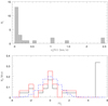 |
Fig. 6. Same as Fig. 4 but for S1 resampled (S1′) so as to mimic the R-sample in terms of Δt and Nobs. |
The small number of observations per star available in sample R forbids us from distinguishing between “jitter” stars and “SB?” stars. Therefore, category “jitter” is no longer considered in method (b).
Both methods (a) and (b) rely on the same premise, namely the “test of equality of two proportions” based on a “contingency table”. A basic description of the principles of this method may be found in for example Sect. 14.4 of Numerical Recipes (Press et al. 2007) or in Agresti (2012). The situation is as follows. Each target star has two different properties associated with it (in our case Li-rich or not-Li-rich and binary or non-binary in the simplest situation), and we want to know whether knowledge of one property gives us any demonstrable advantage in predicting the value of the other property. In other words, we want to know whether or not these quantities are “associated” or “correlated”. For such a pair of variables, the data can be displayed as a “contingency table”, that is, a table whose rows are labelled by the value of one property, and the columns by the value of the other property, and whose entries are non-negative integers giving the number of observed targets for each combination of row and column. We first present the method in the simplified situation expressed above where one property is Li-rich (or not) and the other is SB (or not). This classification scheme defines a 2 × 2 contingency table, as shown in Table 8, where the Li property corresponds to the rows of the contingency table (identified by the subscript x in what follows; each row containing Nx stars), whereas the SB property corresponds to columns (denoted by subscript y in what follows).
Illustration of a 2 × 2 contingency table, where a, b, c, d are integers denoting the number of individuals in the respective cells.
The null hypothesis,
 (6)
(6)
tests the equality of the two proportions p1 = a/Nx1 = p2 = b/Nx2, with a and b defined in Table 8. In our specific situation, this means testing whether the frequency of SB may be considered the same in the Li-rich and non-Li categories. The hypergeometric distribution law then allows one to evaluate the probability of encountering, under the hypothesis that H0 holds true, a distribution as deviant as the one actually observed. The probability of obtaining the value a under H0 is then expressed by
 (7)
(7)
where  is the number of combinations of m objects among n (> m). If the probability of obtaining the value a or a value more deviant than a is low, this means that the observed counts are not consistent with the null hypothesis of equal proportions, and the null hypothesis must be rejected (at a significance level that we specify below). If we assume that the table is ordered in such a way that the first sample is the least numerous (i.e. Nx1 ≤ Nx2, or a + c ≤ b + d) and the first category is the least frequent (i.e. Ny1 ≤ Ny2, or a + b ≤ c + d), then the number a counting the number of individuals in the first sample and in the first category is necessarily somewhere between zero and the minimum of (Nx1, Ny1), or (a + c, a + b). If we further assume that a < μa, where μa is the expected value for a, namely μa = py1 × Nx1 = (a + b) (a + c)/(a + b + c + d), then p1 < p2, and the significance level with which the null hypothesis may be rejected is obtained by summing the hypergeometric probabilities P(n) of Eq. (7) for n going from zero to a. More precisely, for a bilateral test, the null hypothesis may be rejected at a significance level (of approximately4) α if that probability sums up to α/2. This is known as the Fisher exact test for a 2 × 2 contingency table (e.g. Agresti 2012). In cases where the two samples are categorised on more than two parameters, as we do in Table 6 with the four categories “RV constant”, “RV jitter”, “SB?”, and “SB” (method a; for method b, the category “RV jitter” does not exist as the number of data points is too small to distinguish between “RV jitter” and “SB?”), the Fisher test has to be generalised along the same principles as above, but this time using the generalised hypergeometric distribution. However, the number of computations becomes rapidly gigantic; fortunately, there are several calculators available online for computing the significance level when rejecting the null hypothesis for higher-order contingency tables. We used the one available online5, based on the extension of the Fisher test by Freeman & Halton (1951). We discuss the results of the tests in the following sections.
5.5.1. Internal method (a)
The conclusions resulting from the statistical analysis with method (a) are twofold (they are presented in the upper part of Table 6). First, regarding the Li-rich K giants, the comparison of Li-rich and non-Li K giants reveals no significant difference in the binary frequencies between these two groups (since the first-kind risk of erroneously rejecting the H0 hypothesis while it is true is as large as 54.3%). If anything, there even seems to be a deficit of SB among Li-rich K giants, since there are 18.2% large-amplitude binaries among those (2/11), as compared to 46.2% (6/13) in the comparison sample of non Li-rich K giants. However, rather than resulting from an actual deficit of binaries among Li-rich stars (not confirmed by method b; see Sect. 5.5.2), the above imbalance seems to be caused by the fact that the comparison sample of non-Li-rich stars contains several dusty K giants, and this class seems to host an anomalously large number of binaries. Indeed, the analysis of the dusty versus non-dusty contingency table reveals a significant difference in their binary frequencies, with a first-kind risk when rejecting the H0 hypothesis of only 1.6%. Method (b) indeed reveals that this imbalance is caused by the presence of an unusually high frequency of binaries among dusty K giants as compared to the reference sample R (first-kind risk of 3.3% only; Sect. 5.5.2).
The difference between dusty and non-dusty K giants further extends to the jitter category, which is in excess among dusty K giants (37.5%, or 3 stars among 8), as compared to 6.25% or 1/16 among the non-dusty K giants. A likely explanation is that the dusty K giants are on average more luminous than the non-dusty ones and hence more prone to RV jitter, as jitter is known to increase with luminosity (e.g. Mayor et al. 1984; Carney et al. 2003; Hekker et al. 2008). This hypothesis is indeed confirmed by the location of dusty and RV-jitter stars in the HR diagram, as discussed in Sect. 2.2.3 in relation with Fig. 1. Overall, the dusty K giants do not include a single case of constant RV (0/8), and this result is highly significant because 56% (9/16) of the stars in the non-dusty sample are constant-RV stars.
5.5.2. External method (b)
The results from the statistical analysis using method (b) are presented in the lower part of Table 6. It should be read in the following way: 3 × 2 contingency tables were built by combining any of the first lines with the last one corresponding to sample R, and the resulting first-kind risk of rejecting the null hypothesis H0 (that the binary frequency is the same in the two samples being compared) while it is true is listed in the last column.
As already hinted at in Sect. 5.5.1, the comparison with the reference sample R now makes it quite clear that the frequency of binaries in the sample of dusty K giants is significantly higher than in the reference sample of K giants (with a first-kind risk when rejecting the H0 hypothesis of 3.3%), whereas the binary frequency among Li-rich giants is totally normal (with a first-kind risk as high as 73.3%). The high frequency of binaries among non-Li-rich stars simply reflects the larger number of dusty stars among this subsample than among Li-rich giants.
We also note that the binary frequency (SB+SB?) in sample S1′ is almost identical to that in sample S1, namely 10 and 11 stars, respectively, as seen by comparing the lines labelled “Total (S1)” and “Total (S1′)” in Table 6.
5.5.3. Comparison with literature
To conclude this section, it is worth mentioning that the overall binary frequency in sample S1 of 24 K giants, namely 10/24 or 11/24 or 41.7−45.8% (rows Ny1 of Table 6) is higher than that obtained by studying more extended samples, but this may simply reflect the relatively large fraction of dusty K giants in sample S1, and their associated binary nature.
In contrast, sample R has a binary frequency (17.4−23.7%) well in line with that derived by previous studies focusing on K giants. For instance, among 5643 field K giants, Famaey et al. (2005) found 14.5% spectroscopic binaries (with a number of RV points per target of only 2 or 3, comparable to that of sample R), a result in agreement with those of Harris & McClure (1983) (15 to 20% binaries) and of Mermilliod et al. (2007) (16 ± 2% of binaries after 3 RV measurements). The more recent analysis of GES data (Merle et al. 2020), with a SB1 fraction of 21 ± 3% among K giants, confirms the results of all previous analyses, including our present result for sample R binary frequency.
6. Conclusions
The main conclusion of our analysis is that the binary frequency among Li-rich K giants is normal when compared to that found under similar observing conditions in a reference sample of 190 K giants. Therefore, the claim by Casey et al. (2019) that there is a link between binarity and Li excess through tidal effects is not supported by our study, since this would require a 100% frequency of binaries among Li-rich stars, which is clearly not observed. There is also no correlation between Li-richness and the presence of circumstellar dust. The only correlation that could be found between Li enrichment and rapid rotation is that the most Li-enriched K giants appear to be fast-rotating stars. The availability of Gaia parallaxes allowed us to locate the S1 targets in the HR diagram, from which it appears that:
-
The only two long-period binary systems among Li-rich K giants (HD 787 and HD 233517) are not in the red clump but are at a much higher luminosity (either on the RGB or early-AGB).
-
Despite the fact that our S1 sample contains several binary systems in the red clump, none of those among the Li-rich K giants in the red clump are binaries.
-
Three among the four binary (non-Li-rich) stars in the red clump (HD 3627, HD 119853 and HD 212320) are surrounded by cool dust. The five other dusty stars are located along the giant branches (either RGB or early-AGB).
-
The stars with RV jitter (crosses in Figs. 1 and 5) are among the most luminous in the sample, hinting at some intrinsic origin (perhaps non-radial pulsations) for this jitter (see Hatzes et al. 2018, for a recent discussion). Furthermore, those among the most luminous stars which do not exhibit RV jitter show small-amplitude regular RV variations (small red dots in Fig. 1). HD 112127 is a special case since its RV variations are difficult to characterise, simultaneously exhibiting short-period, small-amplitude variations and a long-term velocity drift, sometimes interrupted by some sort of RV jitter (Fig. C.13).
We also find that dusty K giants are either the most luminous among K giants along the RGB or early-AGB, or are binaries located in the red clump.
CoRoT (Convection, Rotation and planetary Transits) is a mini satellite developed by the French Space agency CNES in collaboration with the Science Programmes of ESA, Austria, Belgium, Brazil, Germany and Spain.
The Kepler data for HD 175370 do not support the pulsation hypothesis, and for this reason the presence of a giant-planet companion around that star was privileged by Hrudková et al. (2017). See also Hatzes et al. (2018) for a recent discussion about the difficulty of distinguishing Jupiter-like planets from intrinsic pulsations in the RV variations of K giants.
Instead of 0.055 km s−1 as stated in Sect. 3.
Because of the discrete character of the hypergeometric distribution, this is only approximate, since the anomalous cases at each side of the distribution do not yield exactly the same tail probabilities.
Acknowledgments
Based on observations obtained with the HERMES spectrograph, which is supported by the Research Foundation – Flanders (FWO), Belgium, the Research Council of KU Leuven, Belgium, the Fonds National de la Recherche Scientifique (F.R.S.-FNRS), Belgium, the Royal Observatory of Belgium, the Observatoire de Genève, Switzerland and the Thüringer Landessternwarte Tautenburg, Germany. This work has made use of data from the European Space Agency (ESA) mission Gaia (https://www.cosmos.esa.int/gaia), processed by the Gaia Data Processing and Analysis Consortium (DPAC, https://www.cosmos.esa.int/web/gaia/dpac/consortium). Funding for the DPAC has been provided by national institutions, in particular the institutions participating in the Gaia Multilateral Agreement. This research has made use of the SIMBAD database, operated at CDS, Strasbourg, France. This research has been funded by the Belgian Science Policy Office under contract BR/143/A2/STARLAB, and by the F.W.O. under contract ZKD1501-00-W01. LS and DP are senior research associates at the F.R.S.-FNRS.
References
- Agresti, A. 2012, Categorical Data Analysis, 3rd edn. (Wiley) [Google Scholar]
- Alam, S., Albareti, F. D., Allende Prieto, C., et al. 2015, ApJS, 219, 12 [NASA ADS] [CrossRef] [Google Scholar]
- Angelou, G. C., D’Orazi, V., Constantino, T. N., et al. 2015, MNRAS, 450, 2423 [NASA ADS] [CrossRef] [Google Scholar]
- Baglin, A., Auvergne, M., Barge, P., et al. 2006, in The CoRoT Mission Pre-Launch Status – Stellar Seismology and Planet Finding, eds. M. Fridlund, A. Baglin, J. Lochard, & L. Conroy, ESA Spec. Publ., 1306, 33 [Google Scholar]
- Bakos, G. A. 1976, JRASC, 70, 23 [NASA ADS] [Google Scholar]
- Balachandran, S. C., Fekel, F. C., Henry, G. W., & Uitenbroek, H. 2000, ApJ, 542, 978 [NASA ADS] [CrossRef] [Google Scholar]
- Baranne, A., Mayor, M., & Poncet, J. L. 1979, Vist. Astron., 23, 279 [NASA ADS] [CrossRef] [Google Scholar]
- Barnbaum, C., Stone, R. P. S., & Keenan, P. C. 1996, ApJS, 105, 419 [NASA ADS] [CrossRef] [EDP Sciences] [Google Scholar]
- Bessel, M. S., Castelli, F., & Plez, B. 1998, A&A, 333, 231 [Google Scholar]
- Bharat Kumar, Y., Reddy, B. E., Muthumariappan, C., & Zhao, G. 2015, A&A, 577, A10 [NASA ADS] [CrossRef] [EDP Sciences] [Google Scholar]
- Bharat Kumar, Y., Singh, R., Eswar Reddy, B., & Zhao, G. 2018, ApJ, 858, L22 [NASA ADS] [CrossRef] [Google Scholar]
- Blackwell, D. E., & Lynas-Gray, A. E. 1998, A&AS, 129, 505 [NASA ADS] [CrossRef] [EDP Sciences] [Google Scholar]
- Brown, J. A., Sneden, C., Lambert, D. L., & Dutchover, E., Jr. 1989, ApJS, 71, 293 [CrossRef] [Google Scholar]
- Cardelli, J. A., Clayton, G. C., & Mathis, J. S. 1989, ApJ, 345, 245 [NASA ADS] [CrossRef] [Google Scholar]
- Carlberg, J. K., Cunha, K., Smith, V. V., & Majewski, S. R. 2012, ApJ, 757, 109 [NASA ADS] [CrossRef] [Google Scholar]
- Carney, B. W., Latham, D. W., Stefanik, R. P., Laird, J. B., & Morse, J. A. 2003, AJ, 125, 293 [NASA ADS] [CrossRef] [Google Scholar]
- Casey, A. R., Ruchti, G., Masseron, T., et al. 2016, MNRAS, 461, 3336 [NASA ADS] [CrossRef] [Google Scholar]
- Casey, A. R., Ho, A. Y. Q., Ness, M., et al. 2019, ApJ, 880, 125 [NASA ADS] [CrossRef] [Google Scholar]
- Castilho, B. V., Gregorio-Hetem, J., Spite, F., Spite, M., & Barbuy, B. 1998, A&AS, 127, 139 [NASA ADS] [CrossRef] [EDP Sciences] [Google Scholar]
- Charbonnel, C., & Balachandran, S. C. 2000, A&A, 359, 563 [Google Scholar]
- Charbonnel, C., & Lagarde, N. 2010, A&A, 522, A10 [NASA ADS] [CrossRef] [EDP Sciences] [MathSciNet] [PubMed] [Google Scholar]
- Charbonnel, C., Lagarde, N., Jasniewicz, G., et al. 2020, A&A, 633, A34 [CrossRef] [EDP Sciences] [Google Scholar]
- Cutri, R. M., Wright, E. L., Conrow, T., et al. 2013, VizieR Online Data Catalog: II/328 [Google Scholar]
- da Silva, L., de La Reza, R., & Barbuy, B. 1995, ApJ, 448, L41 [NASA ADS] [CrossRef] [Google Scholar]
- Deepak, & Reddy, B. E. 2019, MNRAS, 484, 2000 [NASA ADS] [Google Scholar]
- de La Reza, R., & da Silva, L. 1995, ApJ, 439, 917 [NASA ADS] [CrossRef] [Google Scholar]
- de La Reza, R., Drake, N. A., & da Silva, L. 1996, ApJ, 456, L115 [NASA ADS] [CrossRef] [Google Scholar]
- de la Reza, R., Drake, N. A., da Silva, L., Torres, C. A. O., & Martin, E. L. 1997, ApJ, 482, L77 [NASA ADS] [CrossRef] [Google Scholar]
- de la Reza, R., Drake, N. A., Oliveira, I., & Rengaswamy, S. 2015, ApJ, 806, 86 [NASA ADS] [CrossRef] [EDP Sciences] [Google Scholar]
- De Medeiros, J. R., & Mayor, M. 1999, A&AS, 139, 433 [NASA ADS] [CrossRef] [EDP Sciences] [Google Scholar]
- De Medeiros, J. R., Melo, C. H. F., & Mayor, M. 1996, A&A, 309, 465 [NASA ADS] [Google Scholar]
- De Medeiros, J. R., do Nascimento, J. D., Jr., Sankarankutty, S., Costa, J. M., & Maia, M. R. G. 2000, A&A, 363, 239 [Google Scholar]
- Denissenkov, P. A., & Herwig, F. 2004, ApJ, 612, 1081 [NASA ADS] [CrossRef] [Google Scholar]
- Drake, N. A., de la Reza, R., da Silva, L., & Lambert, D. L. 2002, AJ, 123, 2703 [NASA ADS] [CrossRef] [Google Scholar]
- ESA 1997, in The HIPPARCOS and TYCHO Catalogues, ESA Spec. Publ., 1200 [Google Scholar]
- Escorza, A., Boffin, H. M. J., Jorissen, A., et al. 2017, A&A, 608, A100 [NASA ADS] [CrossRef] [EDP Sciences] [Google Scholar]
- Escorza, A., Karinkuzhi, D., Jorissen, A., et al. 2019, A&A, 626, A128 [NASA ADS] [CrossRef] [EDP Sciences] [Google Scholar]
- Famaey, B., Jorissen, A., Luri, X., et al. 2005, A&A, 430, 165 [NASA ADS] [CrossRef] [EDP Sciences] [Google Scholar]
- Fekel, F. C., & Watson, L. C. 1998, AJ, 116, 2466 [NASA ADS] [CrossRef] [Google Scholar]
- Fisher, R. S., Telesco, C. M., Piña, R. K., & Knacke, R. F. 2003, ApJ, 586, L91 [NASA ADS] [CrossRef] [EDP Sciences] [Google Scholar]
- Frankowski, A., Jancart, S., & Jorissen, A. 2007, A&A, 464, 377 [NASA ADS] [CrossRef] [EDP Sciences] [Google Scholar]
- Freeman, G. H., & Halton, J. 1951, Biometrika, 38, 141 [CrossRef] [Google Scholar]
- Gaia Collaboration (Brown, A. G. A., et al.) 2018, A&A, 616, A1 [NASA ADS] [CrossRef] [EDP Sciences] [Google Scholar]
- Gezer, I., Van Winckel, H., Bozkurt, Z., et al. 2015, MNRAS, 453, 133 [NASA ADS] [CrossRef] [Google Scholar]
- Gontcharov, G. A. 2006, Astron. Lett., 32, 759 [NASA ADS] [CrossRef] [Google Scholar]
- Gorlova, N., Van Winckel, H., Vos, J., et al. 2013, in EAS Publications Series, eds. K. Pavlovski, A. Tkachenko, & G. Torres, 64, 163 [CrossRef] [EDP Sciences] [Google Scholar]
- Gregorio-Hetem, J., Castilho, B. V., & Barbuy, B. 1993, A&A, 268, L25 [NASA ADS] [Google Scholar]
- Griffin, R. F. 2013, The Observatory, 133, 212 [Google Scholar]
- Gustafsson, B., Edvardsson, B., Eriksson, K., et al. 2008, A&A, 486, 951 [NASA ADS] [CrossRef] [EDP Sciences] [Google Scholar]
- Harris, H. C., & McClure, R. D. 1983, ApJ, 265, L77 [NASA ADS] [CrossRef] [Google Scholar]
- Hatzes, A. P., Endl, M., Cochran, W. D., et al. 2018, AJ, 155, 120 [NASA ADS] [CrossRef] [Google Scholar]
- Hekker, S., & Meléndez, J. 2007, A&A, 475, 1003 [NASA ADS] [CrossRef] [EDP Sciences] [Google Scholar]
- Hekker, S., Snellen, I. A. G., Aerts, C., et al. 2008, A&A, 480, 215 [NASA ADS] [CrossRef] [EDP Sciences] [Google Scholar]
- Hrudková, M., Hatzes, A., Karjalainen, R., et al. 2017, MNRAS, 464, 1018 [NASA ADS] [CrossRef] [Google Scholar]
- Jancart, S., Jorissen, A., Babusiaux, C., & Pourbaix, D. 2005, A&A, 442, 365 [NASA ADS] [CrossRef] [EDP Sciences] [Google Scholar]
- Jasniewicz, G., Parthasarathy, M., de Laverny, P., & Thévenin, F. 1999, A&A, 342, 831 [NASA ADS] [Google Scholar]
- Jordi, C. 2018, Gaia DPAC Report GAIA-C5-TN-UB-CJ-041 [Google Scholar]
- Jorissen, A. 2019, Mem. Soc. Astron. It., 90, 395 [Google Scholar]
- Jorissen, A., Van Eck, S., Van Winckel, H., et al. 2016a, A&A, 586, A158 [NASA ADS] [CrossRef] [EDP Sciences] [Google Scholar]
- Jorissen, A., Hansen, T., Van Eck, S., et al. 2016b, A&A, 586, A159 [NASA ADS] [CrossRef] [EDP Sciences] [Google Scholar]
- Jorissen, A., Boffin, H. M. J., Karinkuzhi, D., et al. 2019, A&A, 626, A127 [NASA ADS] [CrossRef] [EDP Sciences] [Google Scholar]
- Jura, M. 1999, ApJ, 515, 706 [CrossRef] [Google Scholar]
- Jura, M. 2003, ApJ, 582, 1032 [NASA ADS] [CrossRef] [Google Scholar]
- Kamath, D., Wood, P. R., Van Winckel, H., & Nie, J. D. 2016, A&A, 586, L5 [NASA ADS] [CrossRef] [EDP Sciences] [Google Scholar]
- Katz, D., & Brown, A. G. A. 2017, SF2A-2017: Proceedings of the Annual Meeting of the French Society of Astronomy and Astrophysics, held 4–7 July, 2017 in Paris, 259 [Google Scholar]
- Kerschbaum, F., Lebzelter, T., & Mekul, L. 2010, A&A, 524, A87 [NASA ADS] [CrossRef] [EDP Sciences] [Google Scholar]
- Kessler, M. F., Steinz, J. A., Anderegg, M. E., et al. 1996, A&A, 315, L27 [NASA ADS] [Google Scholar]
- Kim, S. S., Zuckerman, B., & Silverstone, M. 2001, ApJ, 550, 1000 [CrossRef] [Google Scholar]
- Kluska, J., Van Winckel, H., Hillen, M., et al. 2019, A&A, 631, A108 [NASA ADS] [CrossRef] [EDP Sciences] [Google Scholar]
- Koch, D. G., Borucki, W. J., Basri, G., et al. 2010, ApJ, 713, L79 [NASA ADS] [CrossRef] [Google Scholar]
- Kumar, Y. B., Reddy, B. E., & Lambert, D. L. 2011, ApJ, 730, L12 [NASA ADS] [CrossRef] [Google Scholar]
- Kumar, B. Y., Reddy, B. E., Muthumariappan, C., & Zhao, G. 2015, A&A, 577, A10 [NASA ADS] [CrossRef] [EDP Sciences] [Google Scholar]
- Lattanzio, J. C., Siess, L., Church, R. P., et al. 2015, MNRAS, 446, 2673 [NASA ADS] [CrossRef] [Google Scholar]
- Lebzelter, T., Uttenthaler, S., Busso, M., Schultheis, M., & Aringer, B. 2012, A&A, 538, A36 [NASA ADS] [CrossRef] [EDP Sciences] [Google Scholar]
- Liu, Y. J., Tan, K. F., Wang, L., et al. 2014, ApJ, 785, 94 [NASA ADS] [CrossRef] [Google Scholar]
- Luck, R. E. 2015, AJ, 150, 88 [Google Scholar]
- Makarov, V. V., & Kaplan, G. H. 2005, AJ, 129, 2420 [NASA ADS] [CrossRef] [Google Scholar]
- Manick, R., Van Winckel, H., Kamath, D., Hillen, M., & Escorza, A. 2017, A&A, 597, A129 [NASA ADS] [CrossRef] [EDP Sciences] [Google Scholar]
- Martell, S. L., & Shetrone, M. D. 2013, MNRAS, 430, 611 [NASA ADS] [CrossRef] [Google Scholar]
- Mayor, M., Imbert, M., Andersen, J., et al. 1984, A&A, 134, 118 [Google Scholar]
- McWilliam, A. 1990, ApJS, 74, 1075 [NASA ADS] [CrossRef] [Google Scholar]
- Merle, T., Jorissen, A., Van Eck, S., Masseron, T., & Van Winckel, H. 2016, A&A, 586, A151 [NASA ADS] [CrossRef] [EDP Sciences] [Google Scholar]
- Merle, T., Van der Swaelmen, M., Van Eck, S., et al. 2020, A&A, 635, A155 [Google Scholar]
- Mermilliod, J.-C., Andersen, J., Latham, D. W., & Mayor, M. 2007, A&A, 473, 829 [NASA ADS] [CrossRef] [EDP Sciences] [Google Scholar]
- Mishenina, T. V., Bienaymé, O., Gorbaneva, T. I., et al. 2006, A&A, 456, 1109 [NASA ADS] [CrossRef] [EDP Sciences] [Google Scholar]
- Mosser, B., Benomar, O., Belkacem, K., et al. 2014, A&A, 572, L5 [NASA ADS] [CrossRef] [EDP Sciences] [PubMed] [Google Scholar]
- Murakami, H., Baba, H., Barthel, P., et al. 2007, PASJ, 59, S369 [NASA ADS] [CrossRef] [MathSciNet] [Google Scholar]
- Neugebauer, G., Habing, H. J., van Duinen, R., et al. 1984, ApJ, 278, L1 [Google Scholar]
- Oomen, G.-M., Van Winckel, H., Pols, O., et al. 2018, A&A, 620, A85 [NASA ADS] [CrossRef] [EDP Sciences] [Google Scholar]
- Plets, H., Waelkens, C., Oudmaijer, R. D., & Waters, L. B. F. M. 1997, A&A, 323, 513 [NASA ADS] [Google Scholar]
- Pourbaix, D., Tokovinin, A. A., Batten, A. H., et al. 2004, A&A, 424, 727 [NASA ADS] [CrossRef] [EDP Sciences] [Google Scholar]
- Press, W. H., Teukolsky, S. A., Vetterling, W. T., & Flannery, B. 2007, Numerical Recipes: The Art of Scientific Computing, 3rd edn. (Cambridge: Cambridge University Press) [Google Scholar]
- Raskin, G., van Winckel, H., Hensberge, H., et al. 2011, A&A, 526, A69 [NASA ADS] [CrossRef] [EDP Sciences] [Google Scholar]
- Rebull, L. M., Carlberg, J. K., Gibbs, J. C., et al. 2015, AJ, 150, 123 [NASA ADS] [CrossRef] [Google Scholar]
- Reddy, B. E., & Lambert, D. L. 2005, AJ, 129, 2831 [NASA ADS] [CrossRef] [Google Scholar]
- Reddy, B. E., Lambert, D. L., Hrivnak, B. J., & Bakker, E. J. 2002, AJ, 123, 1993 [NASA ADS] [CrossRef] [Google Scholar]
- Rowan-Robinson, M. 2000, MNRAS, 316, 885 [Google Scholar]
- Ruchti, G. R., Fulbright, J. P., Wyse, R. F. G., et al. 2011, ApJ, 743, 107 [NASA ADS] [CrossRef] [Google Scholar]
- Siess, L., & Arnould, M. 2008, A&A, 489, 395 [NASA ADS] [CrossRef] [EDP Sciences] [Google Scholar]
- Siess, L., & Livio, M. 1999, MNRAS, 308, 1133 [NASA ADS] [CrossRef] [Google Scholar]
- Siess, L., Dufour, E., & Forestini, M. 2000, A&A, 358, 593 [Google Scholar]
- Singh, R., Reddy, B. E., Bharat Kumar, Y., & Antia, H. M. 2019, ApJ, 878, L21 [NASA ADS] [CrossRef] [Google Scholar]
- Smiljanic, R., Franciosini, E., Bragaglia, A., et al. 2018, A&A, 617, A4 [NASA ADS] [CrossRef] [EDP Sciences] [Google Scholar]
- Stellingwerf, R. F. 1978, ApJ, 224, 953 [NASA ADS] [CrossRef] [Google Scholar]
- Stock, S., Reffert, S., & Quirrenbach, A. 2018, A&A, 616, A33 [NASA ADS] [CrossRef] [EDP Sciences] [Google Scholar]
- Takeda, Y., & Tajitsu, A. 2017, PASJ, 69, 74 [NASA ADS] [Google Scholar]
- Tautvaišienė, G., Barisevičius, G., Chorniy, Y., Ilyin, I., & Puzeras, E. 2013, MNRAS, 430, 621 [NASA ADS] [CrossRef] [Google Scholar]
- Tokovinin, A. 2014, AJ, 147, 87 [NASA ADS] [CrossRef] [Google Scholar]
- Udry, S., Mayor, M., & Queloz, D. 1999, in IAU Colloq. 170: Precise Stellar Radial Velocities, eds. J. B. Hearnshaw, & C. D. Scarfe, ASP Conf. Ser., 185, 367 [NASA ADS] [Google Scholar]
- Van Winckel, H. 2003, ARA&A, 41, 391 [NASA ADS] [CrossRef] [Google Scholar]
- Vos, J., Østensen, R. H., Marchant, P., & Van Winckel, H. 2015, A&A, 579, A49 [NASA ADS] [CrossRef] [EDP Sciences] [Google Scholar]
- Wallerstein, G., & Sneden, C. 1982, ApJ, 255, 577 [NASA ADS] [CrossRef] [Google Scholar]
- Waters, L. B. F. M., Beintema, D. A., Cami, J., et al. 1999, in The Universe as Seen by ISO, eds. P. Cox, & M. Kessler, ESA Spec. Publ., 427, 219 [NASA ADS] [Google Scholar]
- Wilson, E. B., & Hilferty, M. M. 1931, Proc. Natl. Acad. Sci., 17, 684 [NASA ADS] [CrossRef] [Google Scholar]
- Wright, E. L., Eisenhardt, P. R. M., Mainzer, A. K., et al. 2010, AJ, 140, 1868 [NASA ADS] [CrossRef] [Google Scholar]
- Zuckerman, B., Kim, S. S., & Liu, T. 1995, ApJ, 446, L79 [NASA ADS] [CrossRef] [Google Scholar]
Appendix A: Detailed properties of samples S and R
Table A.1 lists all relevant properties for sample S2 of Li-rich K giants collected from Bharat Kumar et al. (2015) and Charbonnel et al. (2020). In Table A.2, all details are provided about sample R consisting in 190 Kepler and CoRoT K giants, serving as reference sample to which the binary frequency among Li-rich giants may be compared.
Sample S2 of Li-rich K giants collected from Bharat Kumar et al. (2015) and Charbonnel et al. (2020).
Sample R (Kepler and CoRoT K giants) and its binary properties (see Sect. 5.1).
Appendix B: SED of dusty stars
This section presents the SED of dusty stars (Figs. B.1−B.9).
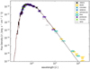 |
Fig. B.1. Spectral energy distribution for HD 3627 with photometry extracted from the SIMBAD data base, with the best-fitting MARCS model superimposed (red curve, barely visible). The black curve corresponds to the dereddened SED. Far-IR excess has been detected by IRAS and AKARI. |
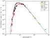 |
Fig. B.5. Same as Fig. B.1 for HD 156115. The SED temperature is 3900 K and the IR excess is doubtful. |
Appendix C: RV curves
This section presents the RV curves of all target stars (Figs. C.1−C.18).
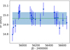 |
Fig. C.1. Radial-velocity data for HD 6. The dashed green line marks the average velocity, and the shaded blue zone corresponds to ±1σ. |
 |
Fig. C.4. Top panel: radial-velocity data for HD 30834. Early measurements with large error bars are from Famaey et al. (2005). Bottom panel: zoom on the HERMES velocities. |
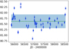 |
Fig. C.6. Radial-velocity data for HD 39853, flagged as a binary by the χ2 test. |
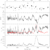 |
Fig. C.7. Period analysis of the RVs using the Stellingwerf statistics. Top panel: RVs plotted in phase with a period of 282 d. Bottom panel: Stellingwerf 1 − θ statistical indicator for a sine signal of period 282 d sampled the same way as HD 39853. Middle bottom panel: same as bottom for the 282 d sine signal (red curve) and for the HD 39853 data (black curve). Middle top panel: the difference between the red and black curve of the previous panel, showing possible residual signals (here one around 110 d). |
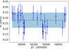 |
Fig. C.10. Same as Fig. C.1 for HD 63798. |
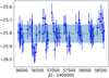 |
Fig. C.11. Same as Fig. C.1 for HD 90633. |
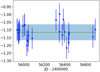 |
Fig. C.12. Same as Fig. C.1 for HD 108741. |
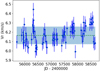 |
Fig. C.13. Same as Fig. C.1 for HD 112127. This star is sometimes classified as a carbon star of type R (Barnbaum et al. 1996). |
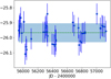 |
Fig. C.14. Same as Fig. C.1 for HD 116292. |
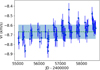 |
Fig. C.15. Same as Fig. C.1 for HD 119853, showing a long-term trend. |
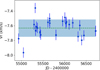 |
Fig. C.16. Same as Fig. C.1 for HD 153687. |
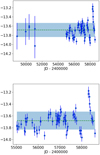 |
Fig. C.17. Same as Fig. C.1 for HD 221776, showing no sign for binarity despite a probability unity of having a variable RV (Table 5). The top panel also displays six RV measurements from Famaey et al. (2005). The bottom panel shows only the HERMES RV. |
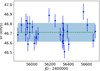 |
Fig. C.18. Same as Fig. C.1 for HD 233517. |
Appendix D: Orbital solutions
This section presents the orbital solutions found so far, displayed in Figs. D.2−D.8, as well as notes on individual stars.
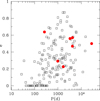 |
Fig. D.1. Eccentricity–period diagram for the new orbits derived in this paper (red filled circles), as compared to the sample of K giants in open clusters (open squares) from Mermilliod et al. (2007). |
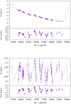 |
Fig. D.2. Top panel: preliminary orbital solution for HD 787 (with the shortest possible orbital period of 4200 d). Bottom panel: orbital solution fitted to the residuals of the top panel. |
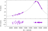 |
Fig. D.3. Same as Fig. D.2 for HD 3627, with a tentative period of the order of 76 yr. The older measurements are from Famaey et al. (2005). |
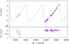 |
Fig. D.6. Same as Fig. D.2 for HD 31553, including Fekel & Watson (1998) measurements. |
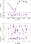 |
Fig. D.7. Top panel: same as Fig. D.2 for HD 156115. Bottom panel: orbital solution fitted to the residuals of the top panel. |
Famaey et al. (2005) data have been used to improve the orbit of the very long-period binary HD 3627. Bakos (1976) proposed a preliminary orbit based on observations spanning 75 years, but only provides a preliminary period of 15 000 d, whereas the Ninth Catalogue of Orbits of Spectroscopic Binaries (Pourbaix et al. 2004) rederived an orbital period of 20 158 d from the observations collected by Bakos (1976).
Griffin (2013) provides for HD 27497 an orbit very similar to that derived from our HERMES data, as listed in Table 4. For HD 31553, measurements from Fekel & Watson (1998) have been added to the HERMES data set in order to better constrain the orbital period, but no zero-point offset has been considered.
HD 21078 (=HIP 15769) is a high proper-motion star (LTT 1604) flagged as an acceleration solution (DMSA/G) in the Double and Multiple Star Annex of the HIPPARCOS catalogue (ESA 1997). It is also a so-called Δμ binary (long-term Tycho-2 and short-term HIPPARCOS proper motions are discrepant) flagged by Makarov & Kaplan (2005) and Frankowski et al. (2007). We computed a combined HERMES/HIPPARCOS spectroscopic/astrometric solution following the method outlined by Jancart et al. (2005). All significance tests described in the latter paper are satisfied, indicating the good quality of the combined orbit whose elements are listed in Table 4c. We also note the good agreement between the dynamical parallax of 13.3 ± 1.1 mas (Table 4c) and the Gaia DR2 parallax of 12.5 ± 0.1 mas (Table 2). The knowledge of the orbital inclination allows us to derive pairs of possible (M1, M2) values (listed in Table 4c) from the spectroscopic mass function. The location of HD 21078 in the HR diagram (Sect. 2.2.3) points at a mass ∼1.2 M⊙ for component A, and therefore the companion must have a mass of 0.71 M⊙. Such a mass is compatible with the companion being either a main-sequence star or a white dwarf (the latter possibility is less likely since the K giant should then appear as a barium star, which it is not; see Merle et al. 2016). The low-mass of the companion implies that it contributes negligible light to the system, and therefore the photocentre location must be identical with the giant location. Hence the semi-major axis of the giant around the centre of mass of the system (a1) must be identical with the semi-major axis of the photocentric orbit (a0), as confirmed from Tables 4a,c.
Figure D.1 presents the eccentricity–period diagram for the new orbits derived in this paper (red filled circles), and is compared to the sample of K giants in open clusters from Mermilliod et al. (2007). All binaries from sample S1 fall within the locus occupied by the binary K giants in open clusters (even though HD 21078 lies along its boundary; this is compatible with the fact that HD 21078 is a subgiant rather than a giant – as revealed by Fig. 1 – and therefore the tidal orbital circularisation has not yet operated). Therefore, there is nothing peculiar to report about the orbital dynamics of our sample stars.
All Tables
Comparison between the stellar parameters derived in this study (Table 2) with their Bayesian estimates from Stock et al. (2018).
Binary properties of sample S1 ordered by increasing RV standard deviation σj(RV).
Contingency tables testing the correlation between binarity frequency and dusty or Li-rich nature.
Illustration of a 2 × 2 contingency table, where a, b, c, d are integers denoting the number of individuals in the respective cells.
Sample S2 of Li-rich K giants collected from Bharat Kumar et al. (2015) and Charbonnel et al. (2020).
Sample R (Kepler and CoRoT K giants) and its binary properties (see Sect. 5.1).
All Figures
|
Fig. 1. Li-rich (large filled dots) and dust-rich (open squares) K giants from sample S1 in the HR diagram. Small filled dots are non-Li-rich K giants. Green symbols denote SB, as discussed in Sect. 5. Small red dots indicate the presence of regular small-amplitude variations, whereas large crosses indicate irregular small-amplitude variations (RV jitter). STAREVOL tracks (Siess et al. 2000; Siess & Arnould 2008) are labelled according to their initial mass, and correspond to solar metallicity. Tracks evolving along the core He-burning phase are depicted in blue, whereas tracks along the AGB are displayed in red. The red clump as defined by Deepak & Reddy (2019; their Fig. 1) is represented by the dashed rectangle. The bump is well visible on the 1 M⊙ track as the hook feature located to the lower right of the red clump region. |
| In the text | |
|
Fig. 2. Top panel: distribution of the number of observations per star in sample R. Bottom panel: number of HERMES observations vs. time span of the RV observations for the comparison sample of Kepler/CoRoT giants (sample R; open squares). Most of the stars have three observations spanning 300 to 900 d. Red crosses correspond to the re-sampled data of sample S1 (denoted ‘sample S1’) with Nobs and Δt modified to mimic the distribution of sample R (see Sect. 5.5). |
| In the text | |
|
Fig. 3. Top panel: distribution of HERMES σj(RV) per star j of the reference sample (R) of CoRoT/Kepler K giants. Bottom: F2j distribution for the same sample. In black is drawn the full sample, and in red the sample with binaries removed (F2 ≥ 3.0), which leads to an almost perfect match between the binary-free observed F2 distribution (red curve) and the expected 𝒩(0, 1) normal-reduced distribution (blue curve). |
| In the text | |
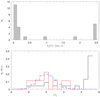 |
Fig. 4. Same as Fig. 3 but for sample S1. |
| In the text | |
|
Fig. 5. Radial-velocity standard deviation (σ(RV), or σ(O−C) in case of orbital SBs) vs. luminosity for sample S1. Symbols are as follows: filled squares show stars with small-amplitude variations, large open circles signify SBs, crosses represent stars showing jitter, open squares show stars with no special features. We note that the jitter stars and those with small-amplitude RV variations are among the most luminous ones, as expected. |
| In the text | |
|
Fig. 6. Same as Fig. 4 but for S1 resampled (S1′) so as to mimic the R-sample in terms of Δt and Nobs. |
| In the text | |
|
Fig. B.1. Spectral energy distribution for HD 3627 with photometry extracted from the SIMBAD data base, with the best-fitting MARCS model superimposed (red curve, barely visible). The black curve corresponds to the dereddened SED. Far-IR excess has been detected by IRAS and AKARI. |
| In the text | |
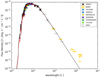 |
Fig. B.2. Same as Fig. B.1 for HD 30834. |
| In the text | |
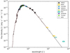 |
Fig. B.3. Same as Fig. B.1 for HD 119853. |
| In the text | |
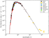 |
Fig. B.4. Same as Fig. B.1 for HD 153687. |
| In the text | |
|
Fig. B.5. Same as Fig. B.1 for HD 156115. The SED temperature is 3900 K and the IR excess is doubtful. |
| In the text | |
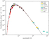 |
Fig. B.6. Same as Fig. B.1 for HD 212320. |
| In the text | |
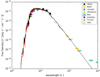 |
Fig. B.7. Same as Fig. B.1 for HD 221776. |
| In the text | |
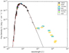 |
Fig. B.8. Same as Fig. B.1 for HDE 233517. The SED temperature is 4211 K. |
| In the text | |
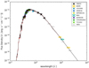 |
Fig. B.9. Same as Fig. B.1 for HD 6, which does not exhibit any IR excess. |
| In the text | |
|
Fig. C.1. Radial-velocity data for HD 6. The dashed green line marks the average velocity, and the shaded blue zone corresponds to ±1σ. |
| In the text | |
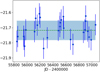 |
Fig. C.2. Same as Fig. C.1 for HD 6665. |
| In the text | |
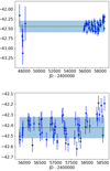 |
Fig. C.3. Top panel: same as Fig. C.1 for HD 9746. Bottom panel: zoom on the HERMES data. |
| In the text | |
|
Fig. C.4. Top panel: radial-velocity data for HD 30834. Early measurements with large error bars are from Famaey et al. (2005). Bottom panel: zoom on the HERMES velocities. |
| In the text | |
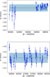 |
Fig. C.5. Same as Fig. C.4 for HD 34043. |
| In the text | |
|
Fig. C.6. Radial-velocity data for HD 39853, flagged as a binary by the χ2 test. |
| In the text | |
|
Fig. C.7. Period analysis of the RVs using the Stellingwerf statistics. Top panel: RVs plotted in phase with a period of 282 d. Bottom panel: Stellingwerf 1 − θ statistical indicator for a sine signal of period 282 d sampled the same way as HD 39853. Middle bottom panel: same as bottom for the 282 d sine signal (red curve) and for the HD 39853 data (black curve). Middle top panel: the difference between the red and black curve of the previous panel, showing possible residual signals (here one around 110 d). |
| In the text | |
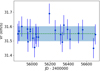 |
Fig. C.8. Same as Fig. C.1 for HD 40827. |
| In the text | |
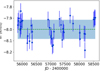 |
Fig. C.9. Same as Fig. C.1 for HD 43827. |
| In the text | |
|
Fig. C.10. Same as Fig. C.1 for HD 63798. |
| In the text | |
|
Fig. C.11. Same as Fig. C.1 for HD 90633. |
| In the text | |
|
Fig. C.12. Same as Fig. C.1 for HD 108741. |
| In the text | |
|
Fig. C.13. Same as Fig. C.1 for HD 112127. This star is sometimes classified as a carbon star of type R (Barnbaum et al. 1996). |
| In the text | |
|
Fig. C.14. Same as Fig. C.1 for HD 116292. |
| In the text | |
|
Fig. C.15. Same as Fig. C.1 for HD 119853, showing a long-term trend. |
| In the text | |
|
Fig. C.16. Same as Fig. C.1 for HD 153687. |
| In the text | |
|
Fig. C.17. Same as Fig. C.1 for HD 221776, showing no sign for binarity despite a probability unity of having a variable RV (Table 5). The top panel also displays six RV measurements from Famaey et al. (2005). The bottom panel shows only the HERMES RV. |
| In the text | |
|
Fig. C.18. Same as Fig. C.1 for HD 233517. |
| In the text | |
|
Fig. D.1. Eccentricity–period diagram for the new orbits derived in this paper (red filled circles), as compared to the sample of K giants in open clusters (open squares) from Mermilliod et al. (2007). |
| In the text | |
|
Fig. D.2. Top panel: preliminary orbital solution for HD 787 (with the shortest possible orbital period of 4200 d). Bottom panel: orbital solution fitted to the residuals of the top panel. |
| In the text | |
|
Fig. D.3. Same as Fig. D.2 for HD 3627, with a tentative period of the order of 76 yr. The older measurements are from Famaey et al. (2005). |
| In the text | |
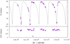 |
Fig. D.4. Same as Fig. D.2 for HD 21078. |
| In the text | |
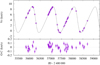 |
Fig. D.5. Same as Fig. D.2 for HD 27497. |
| In the text | |
|
Fig. D.6. Same as Fig. D.2 for HD 31553, including Fekel & Watson (1998) measurements. |
| In the text | |
|
Fig. D.7. Top panel: same as Fig. D.2 for HD 156115. Bottom panel: orbital solution fitted to the residuals of the top panel. |
| In the text | |
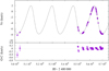 |
Fig. D.8. Same as Fig. D.2 for HD 212320. |
| In the text | |
Current usage metrics show cumulative count of Article Views (full-text article views including HTML views, PDF and ePub downloads, according to the available data) and Abstracts Views on Vision4Press platform.
Data correspond to usage on the plateform after 2015. The current usage metrics is available 48-96 hours after online publication and is updated daily on week days.
Initial download of the metrics may take a while.