| Issue |
A&A
Volume 638, June 2020
|
|
|---|---|---|
| Article Number | A103 | |
| Number of page(s) | 16 | |
| Section | Interstellar and circumstellar matter | |
| DOI | https://doi.org/10.1051/0004-6361/202037554 | |
| Published online | 23 June 2020 | |
Searching for central stars of planetary nebulae in Gaia DR2★
Institute of Astronomy, University of Cambridge,
Madingley Road,
Cambridge,
CB3 0HA,
UK
e-mail: njc89@cam.ac.uk; naw@ast.cam.ac.uk
Received:
22
January
2020
Accepted:
17
April
2020
Context. Accurate distance measurements are fundamental to the study of planetary nebulae (PNe) but they have long been elusive. The most accurate and model-independent distance measurements for galactic PNe come from the trigonometric parallaxes of their central stars, which were only available for a few tens of objects prior to the Gaia mission.
Aims. The accurate identification of PN central stars in the Gaia source catalogues is a critical prerequisite for leveraging the unprecedented scope and precision of the trigonometric parallaxes measured by Gaia. Our aim is to build a complete sample of PN central star detections with minimal contamination.
Methods. We developed and applied an automated technique based on the likelihood ratio method to match candidate central stars in Gaia Data Release 2 (DR2) to known PNe in the Hong Kong/AAO/Strasbourg Hα PN catalogue, taking into account the BP – RP colours of the Gaia sources as well as their positional offsets from the nebula centres. These parameter distributions for both true central stars and background sources were inferred directly from the data.
Results. We present a catalogue of over 1000 Gaia sources that our method has automatically identified as likely PN central stars. We demonstrate how the best matches enable us to trace nebula and central star evolution and to validate existing statistical distance scales, and we discuss the prospects for further refinement of the matching based on additional data. We also compare the accuracy of our catalogue to that of previous works.
Key words: astrometry / methods: statistical / parallaxes / planetary nebulae: general
Table B.1 is only available at the CDS via anonymous ftp to cdsarc.u-strasbg.fr (130.79.128.5) or via http://cdsarc.u-strasbg.fr/viz-bin/cat/J/A+A/638/A103
© ESO 2020
1 Introduction
Planetary nebulae (PNe) are an end stage of life for low and intermediate mass stars, representing a relatively short step on their evolutionary path after their departure from the tip of the asymptotic giant branch (AGB) (Herwig 2005). The star sheds its outer layers, growing brighter and hotter before ultimately cooling into a white dwarf. Ultraviolet light from the star ionises this rapidly expanding shell of gas, which reaches typical sizes of the order of light-years over the tens of thousands of years during which it is visible.
PNe are important in galactic evolution for their enrichment of the interstellar medium (ISM) with heavier elements (Johnson 2019; Karakas & Lattanzio 2014), joining other mechanisms of stellar mass loss such as supernovae. Their brightness and resulting visibility over large distances make PNe valuable chemical probes of not only the Milky Way but also nearby galaxies (Kwitter et al. 2014). In addition, the planetary nebula luminosity function (PNLF) forms a useful rung in the cosmic distance ladder (Ciardullo 2012).
The number of PNe present in our galaxy at any given time is small relative to the stellar population on account of their short lifespans. However the set of 3500 or so confirmed and likely PNe that have been discovered only represents a fraction of those expected to be visible if all stars in a certain mass range go through the PN phase (Moe & De Marco 2006). This inconsistency leaves open questions as to whether there are further requirements for PN formation, namely binary interactions (Jones & Boffin 2017). Our understanding of PNe is limited, in part, by difficulties in constraining their distances (Smith 2015). Accurate distances are critical for a meaningful astrophysical characterisation of PNe. Such characterisation ranges from the measurement of physical sizes and absolute central star magnitudes of individual objects to the determination of lifetimes and formation rates in the population as a whole.
The rapid evolution of Central Stars of PNe (CSPNe) generally prevents the application of usual methods of distance determination such as isochrone fitting. Thus a variety of distance measurement techniques have been developed, which fall into two broad categories (following Frew et al. 2016, henceforth FPB16).
Primary techniques measure the distances to individual PNe with varying degrees of accuracy and assumptions. Most involve modelling – either of the nebula’s expansion (Schönberner et al. 2018), of the environment (e.g. extinction distances, cluster or bulge membership, or location in external galaxies), or of the CSPN itself. The most direct primary distances measurements come from trigonometric parallaxes of CSPNe, but until recently these have only been available for few nearby objects with measurements from the United States Naval Observatory (USNO) (Harris et al. 2007) and the Hubble Space Telescope (HST) (Benedict et al. 2009).
Secondary, or statistical distance scales, rely on finding a broadly applicable relationship that provides a means of estimating a physical parameter of the PN such as its physical size, given a distance-independent measurement, such as nebula surface brightness. The distance can then be determined from the relation of the physical parameter to a measured one, for example through the comparison of physical to angular size, in a manner analogous to the distance modulus for stars with known absolute magnitudes. The determination of the relationships underlying such secondary methods requires a calibrating set of objects whose distances are known independently.
Most PN distance estimates rely on secondary methods, but these methods are only as good as the quality and purity of the distances used to calibrate them. Incorrect distances or polluting objects can inflate errors well beyond the uncertainties stemming from measurement errors and intrinsic scatter. Thus, improved primary distances to a set of PNe provides a twofold benefit, as it betters not only the distances to that set of objects but also, through improved calibration of statistical distance scales, to the population as a whole.
Good primary distance measurements are rare. In their statistical distance scale calibration, FPB16 deemed only around 300 galactic and extragalactic PNe to have sufficiently reliable primary distances. The galactic selection they chose represented only around 5% of confirmed galactic PNe, and their more relatively accurate primary distances were for extragalactic objects.
However, the situation is now changing with the recently launched Gaia mission (Gaia Collaboration 2016b), which is conducting astrometric measurements – positions, parallaxes, and proper motions – of over a billion stars in the Milky Way, including many CSPNe. Stanghellini et al. (2017) found a small number of CSPNe with parallax measurements in Gaia DR1 (Gaia Collaboration 2016a), while Kimeswenger & Barría (2018) found a larger sample in the most recent Gaia data release, DR2 (Gaia Collaboration 2018b), using a manual matching technique and a limited input catalogue. Most recently, González-Santamaría et al. (2019) and Stanghellini et al. (2020) searched Gaia DR2 using more complete input catalogues, but relied on a position-based matching approach that creates a risk of contamination.
Fully exploiting the data from Gaia for the study of PNe requires a CSPN sample that is both complete and pure, which is time-consuming and difficult to achieve manually. As astronomical datasets become larger and are updated more frequently, automated techniques become increasingly useful, offering not only improved speed and consistency but also adaptability, making it easier to incorporate new data as they become available. In the case of Gaia, future data releases will have more detections with improved photometry and parallaxes, so an automated technique will allow these to quickly be taken advantage of.
Our work aims to provide a more complete sample of CSPNe in Gaia DR2 and to lay the groundwork for future data releases, through an automated matching process that we have developed that takes into account both relative position and colour information of Gaia sources. In the remainder of this work we present the technique, the resulting catalogue of CSPNe in Gaia DR2, a comparison of this catalogue to previous works, and finally some initial applications that use the subsets of this catalogue with the most accurate Gaia parallaxes for astrophysical characterisation and distance scale evaluation.
2 Methods
Our starting point is the Hong Kong/AAO/Strasbourg Hα (HASH) PN catalogue1 from Parker et al. (2016). This catalogue represents the most complete catalogue of PNe available, containing at the time of writing2 around 2500 spectroscopically confirmed PNe (following the criteria in Frew & Parker 2010) and 1000 possible and likely PNe, as well as objects that are commonly confused with PNe, such as HII regions, symbiotic stars, and reflection nebulae. HASH also collects together additional information about individual nebulae such as fluxes, angular sizes, and spectra; however it lacks structured positional data on known CSPNe.
PN catalogues have historically suffered from positional inaccuracies. Some uncertainty is intrinsic to PNe as extended objects: they have varied morphologies, and the full extents of their nebulae may not be visible, so different assessments of the nebula position are possible. Moreover in the cases where there is a known or apparent central star, some catalogues adopt this star’s position as that of the PN, though the nebula and star positions can have significant offsets.
In the Macquarie/AAO/Strasbourg Hα PNe catalogue (MASH) (Parker et al. 2006; Miszalski et al. 2008), the precursor to HASH, the authors based their reported positions on the geometric centre of the visible nebula, and claimed uncertainties of the order of 1′′ –2′′. They found notable disagreements between their measured positions for known PNe and those in existing catalogues. This can in part be due to catalogue inhomogeneity noted above. However outright misidentification can also occur, particularly for compact PNe: the HASH authors found positions in the online SIMBAD database that were simply incorrect. We see in Sect. 3.1 that such errors are still present.
HASH promises a homogeneous set of PN coordinates, primarily based on centroiding narrowband Hα imagery of the PNe. This along with its completeness motivates our choice of it as an input catalogue. A disadvantage is that the coordinates contained in the catalogue may not correspond to the central star coordinates even for PNe with known central stars. Information about CSPNe is scattered across the literature and often the coordinates themselves are not identified, even for CSPNe that have been studied (Weidmann & Gamen 2011).
In addition to astrometric parameters (positions, parallaxes, and proper motions), the Gaia satellite measures fluxes in three bands: the wider G band covering visible wavelengths and extending partway into the near infrared (330 to 1050nm), and narrower bands GBP and GRP, covering theblue and red halves of the spectrum respectively (Evans et al. 2018). For well-behaved sources the BP (blue photometer) and RP (red photometer) fluxes essentially add to produce the total flux in G, with this degeneracy giving a single measurement of colour as the magnitude difference across any two passbands (e.g. BP – RP).
The manner in which the BP and RP fluxes are measured makes them more susceptible to contamination by nearby sources or errors in background estimation, particularly in densely populated or nebulous regions. Departures from the expected relation between these fluxes and the flux in G are indicated by the flux excess factor published in the Gaia catalogue; in extreme cases photometry is published for the G band only.
The second Gaia data release, DR2, contains around 1.7 billion sources. About 1.3 billion sources have full sets of astrometric parameters (as opposed to positions only) and a similar number (1.4billion) have full photometry from which colour information can be derived (rather than magnitude in G only).
Not all CSPNe will appear as sources in Gaia DR2, for a variety of possible reasons: appearing too faint (CSPNe can have high bolometric luminosities but emit most of their light in the ultraviolet), having insufficiently many detections, or being obscured by foreground stars, interstellar dust, or the nebula itself. Indeed the fraction of PNe with secure CSPN identifications is small: Parker & Frew (2011) noted it as 25%.
CSPNe that are detected may not be the closest sources to the centre of the visible nebula, especially if the full extent of the nebula is not apparent, or in high density regions such as the galactic centre and plane. PN progenitors are hot (blue) stars, but they may not appear blue in the Gaia BP – RP colour space, due to reddening effects or, in the case of binary CSPNe, the presence of a main sequence or giant companion whose light dominates. With binary systems we are still interested in the detected companion as it provides an equally useful parallax measurement. Some bright and compact PNe may themselves appear like stellar sources, though their spectra will be dominated by nebular emission rather than stellar continuum. Again such sources are useful to detect, and we attempt to match them, though they are not, strictly speaking, CSPNe.
For many if not most PNe, our expectation is that the true central star, if it is visible, will be closest to the centre of the nebula. However, many CSPNe will not be detected by Gaia, and in those cases the closest stars to the nebula centre will be field stars. Our goal is as much to avoid these impostors as it is to recover true CSPNe, as their inclusion skews any further analysis based on their properties. Thus, a matching approach is required that considers more than just taking the nearest neighbour in the Gaia DR2 catalogue for each PN in HASH.
2.1 Catalogue matching
We treat the search for CSPNe as a catalogue matching problem, one of finding correspondences between known PNe and sources in Gaia DR2. The problem of catalogue matching arises often in astronomy, usually in the context of matching objects detected at different wavelengths. It has been well studied, and has a common solution, the likelihood ratio method (Sutherland & Saunders 1992, henceforth SS92), which provides a principled statistical approach towards determining the reliability of candidate matches. We briefly describe the method here for reference, following SS92.
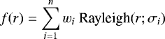
We suppose that we have a sparse primary catalogue and a dense secondary catalogue, and wish to match objects between them. Given a pair of candidate counterparts in two different catalogues, the idea of the likelihood ratio method is to compare two competing hypotheses: the objects are actually the same (a genuine match), or merely coincidental. In the simplest version, if the positions in the catalogues are offset from each other by an angular separation r, the likelihood ratio is the ratio of the probability of finding true counterparts with measured positions separated by r to the probability of finding chance objects with that separation. That is, the likelihood ratio is a ratio of two probability densities. If we assume that Gaussian positional uncertainties are present only in the second catalogue, with standard deviation σ, the distribution of separations follows a Rayleigh distribution with parameter σ. Likewise, assuming a constant background density ρ, the density of spurious objects at a radial separation r from the primary source position simply increases linearly with r (considering a narrow ring of increasing radius). This gives a likelihood ratio3
 (1)
(1)
The likelihood ratio can also incorporate additional properties such as colour and magnitude as well as the prior probability of finding a match. If we consider the colour c in addition to separation r, and furthermore assume that they are independent, we get
 (2)
(2)
where Q is the prior probability of there being a match for the object in the secondary catalogue.
While the likelihood ratio is valid for individual sources in isolation, we should consider the likelihood ratios for all candidate matches together for given primary catalogue object. This is done through the reliability, which for the ith candidate is
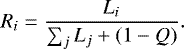 (3)
(3)
Reliability serves as the probability of a match being correct, with the nice properties that the sum of reliabilities of all candidate matches for a given object is at most 1, and the expectation of that sum is the identification rate Q.
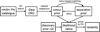 |
Fig. 1 Outline of the steps used in the matching process. |
2.2 Likelihood ratio method for CSPNe
In our approach we take HASH as the primary, or leading, catalogue, and the far denser Gaia DR2 catalogue as the secondary catalogue. We consider the BP – RP colour of Gaia sources in addition to their positional offsets, motivated by the expectation of PN progenitor stars being hotter and thus having identifiably bluer colours.
The main obstacle to applying the likelihood ratio method is the lack of well-characterised positional uncertainties. Determining priors for colour or other parameters in general does not require a set of verified counterparts, and can be done empirically, using methods such as those in SS92 and Salvato et al. (2018), which we describe later.
Our approach is iterative, involving first determining an approximate colour prior based on a simple positional cross-match. Using this prior, we select a new set of counterparts that have high confidence based on colour alone. The angular separations of these counterparts are used to determine positional uncertainties, which in turn are used to generate an improved colour prior to be used in the final matching (Fig. 1).
Though not a strict application of the method, this approach borrows some of the ideas of the co-training technique used in semi-supervised learning (Blum & Mitchell 1998), in which classifiers based on different views of a set of data label examples in order to train each other. It can also be seen as considering the colour and separation terms in Eq. (2) separately and alternating between them.
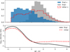 |
Fig. 2 Histogram of BP – RP colours for three different sets of Gaia sources covering both iterations of the colour density ratio computation. The grey histogram shows the distribution of colours of background sources, which does not change visibly between iterations. The initial colour distribution derived from nearest neighbouring sources is indicated by the red dashed line. The colour distribution of the final selection based on separation is indicated in blue. Lower panel: density ratio in colour space, also for both iterations, with the final density ratio indicated by the black line, and the initial ratio derived from nearest versus non-nearest neighbours shown by the dashed red line. All densities are for sources with a well-behaved BP/RP excess factor (indicating reliable colour measurements). |
2.2.1 Nearest neighbour selection
We selected all Gaia sources within 60′′ of the roughly 2500 confirmed PNe in HASH (PNstat=T). We took the closest Gaia source to each PN location (applying a generous separation cutoff of half the PN radius plus 2′′), and compared the empirical distribution of BP – RP colours of these nearest neighbour sources with the other (non-nearest neighbour) sources (sources with no BP – RP colour are ignored in this selection). A simplified version of this comparison is shown in Fig. 2.
In practice we used kernel density estimation rather than the histograms directly, in order to produce a smooth density ratio function, and also consider the BP/RP excess factor as in indicator of the uncertainty in the colour measurement. More details can be found in Appendix A.1.
While the caveats we mentioned previously apply, we do expect that most true central stars will be the nearest sources to the PN centres, and that a significant fraction of nearest neighbours will indeed be true central stars. Thus the nearest neighbour and non-nearest neighbour colour distributions should approximate P(c|genuine) and P(c|chance), with some contamination in both directions. The effect of the contamination is to push the ratio of these densities towards unity, but the structure should still be preserved.
S92 suggest a similar approach based on taking all possible counterparts within a 3σ positional error ellipse, and subtracting from the derived density a representative sample of background objects to account for the expected contamination. The equivalent here would be to subtract the non-nearest neighbour colour distribution from the nearest neighbour one, though we deem this unnecessary for our application.
We used this initial colour prior to select the subset of Gaia sources within our radius cutoff (not necessarily nearest neighbours) that are high confidence matches based on colour alone. In cases with multiple sources with strongly suggestive colours for a single PN, we took the source with the smallest angular separation.
We assume that, for true counterparts, the apparent colour of the CSPN, which may be affected by extinction or binarity, and its position relative to the nominal centre of its PN are independent of each other4 . Under this assumption, the positional distribution of these colour-selected counterparts should be representative of the positional distribution of all true counterparts, and we can use the former as an estimate of the latter. This is what we do in the next step.
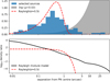 |
Fig. 3 Histogram of the separations of the “high-confidence” sources (selected by colour) from their PN centres, along with, for comparison, a Rayleigh distribution with a similar mode in red, and a uniform density of background sources in grey. Lower panel: separation density ratio resulting from the derived mixture of Rayleigh distributions compared to that from the single Rayleigh distribution in the upper panel. In practice the mixture is re-weighted depending on the radius of the PN. |
2.2.2 Positional uncertainty and background density estimation
The angular separations between the sources selected by colour and their PN centres (upper half of Fig. 3) range from fractions of an arcsecond to tens of arcseconds, and the concentration of very nearby sources combined with the long tail is not well described by a single Rayleigh distribution as in Eq. (1). This is not unexpected as there are many possible sources of disagreement between the PN position in the input catalogue and the position measured by Gaia of its central star. Catalogue positional uncertainties depend on whether the position is that of the nebula centre or of the central star itself. Uncertainties in Gaia source positions vary as well, though we expect these to be negligible relative to other sources of uncertainty. Proper motion can contribute to disagreements if measurement times differ significantly. Finally, even if the catalogue position is accurate, there may be an inherent offset between the central star position and that of the nebula centre.
Thus to estimate the distribution of PN centre separations for true CSPNe, P(r|genuine), we fitted a mixture of Rayleigh distributions, with one distribution per PN – Gaia source pair in our colour selection. Each individual distribution was fitted to the maximum likelihood parameter for the angular separation between the Gaia source and the PN centre. This construction approach simplifies the estimate and ensures the separation density ratio is smooth, strictly decreasing, and behaveswell near zero.
Some sources of uncertainty are dependent on the nebula size. Thus we re-weighted the mixture to reflect offsets to CSPNe for PNe of similar sizes. For example, for a PN with a radius of 60′′ the mixture will be be dominated by PN – Gaia source pairs where the radius of the PN is between around 30′′ and 120′′.
The other component of the term in the angular separation likelihood ratio is the density of background sources, ρ. We estimated this locally for each PN by counting the Gaia sources found within the 60′′ search window. We chose this approach over other methods (e.g. taking the separation to the nth nearest object) for its simplicity. The background source density will be the same for all candidate CSPNe for a given PN, so it does not affect the relative ranking, only the confidence.
2.2.3 Colour prior refinement
The derived positional uncertainties were in turn used to generate a new colour prior, in a manner similar to the “self-constructed priors” described in Salvato et al. (2018). The idea is to derive priors based on the properties of counterparts who identification is reasonably secure based on position alone. Instead of nearest and non-nearest neighbours, we now used the colours of positionally selected CSPNe and non-CSPNe to determine P(c|genuine) and P(c|chance) respectively, leaving out sources for which the position by itself is inconclusive5. This removed many of the contaminants from the previous estimation based on nearest neighbour, showing a stronger preference for blue colours and a decreased score assigned to redder Gaia sources – in essence, increasing the contrast in the colour density ratio function.
In principle we could have alternated back and forth between updating the distances and colour distributions, but the updated colour prior does not significantly change which sources meet the threshold used for the selection at the end of Sect. 2.2.1. Thus further iteration is not necessary.
2.2.4 Final steps
The final piece of the likelihood ratio function is Q, the identification rate. This scales all likelihood ratios, but does not change the ranking. We chose a value for Q of 0.5, to be verified later.
We calculated the likelihood ratios for all Gaia sources within each 60′′ search window, though in selecting matches we enforced an additional separation cutoff of half the radius of the PN plus 2′′ . We did this for all confirmed, likely, and possible PNe in HASH, though only the confirmed PNe were used in deriving the priors. Sources missing BP – RP colours in Gaia had likelihood ratios computed based on position only, equivalent to having the colour term in the likelihood ratio being equal to 1. Following SS92, we computed the reliability of candidate sources for each PN, using that as our scoring metric.
3 Matching results
The reliability distribution of the highest ranked candidate for each PN is strongly bimodal (Fig. 4, upper left), meaning that for most PNe our method has either selected a single Gaia source as the best central star candidate with high confidence or rejected all nearby sources. The mean sum of reliabilities for the 2480 confirmed PNe in HASH is 0.53, consistent with our chosen value of Q6. We focus the remainder of our analysis on these confirmed PNe, as they are most relevant for scientific applications.
Based on the shape of the reliability distribution, we chose 0.8 as our threshold for likely matches and 0.2 as our threshold for possible matches. Applying these thresholds, we find 1086 likely matches and 381 possible matches, representing 44% and 15% respectively of the total number of confirmed PNe.
The highest confidence matches are Gaia sources that are both blue and within fractions of an arcsecond of the HASH position. However either of these criteria alone can be sufficient; our method also finds more distant blue sources and accepts red sources thatare very central (Fig. 4, upper right).
The greatest matching success rates are for extended PNe away from the galactic centre and away from the disc (lower half of Fig. 4), where the PNe tend to be nearer, the density of background objects lower, and the visible light from stars less reddened by dust. Most of the uncertain matches are towards the galactic centre; cursory inspection of these shows that many are missing colours in Gaia and that their positional offsets are too large to accept the candidates based on position alone. These could benefit from the incorporation of additional photometry from other surveys such as VPHAS+ (Drew et al. 2014), spectroscopic followup, or, for those that do have Gaia colours, reddening estimates. It is interesting to observe that few PNe have multiple plausible candidate CSPNe; the choice is generally between a single best candidate and the conclusion that the CSPN as not been detected by Gaia at all.
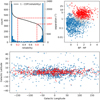 |
Fig. 4 Matching results for confirmed PNe in HASH. The histogram on the upper left shows the reliabilities of highest ranked candidate central stars for each PN. Over-plotted is the mirrored cumulative distribution function (CDF) of that distribution, with the cutoffs and counts for best and potential matches highlighted. The two scatter plots show the distribution of the matches in colour/separation space and in galactic coordinates, with blue circles being likely matches, grey circles being possible matches, and red circles being rejected sources. Larger circles correspond to PN with larger angular sizes. |
3.1 Comparison with previous works
It is difficultto find large samples of positions of verified CSPNe in the literature that would serve as a ground truth to which to compare our matching results. Kerber et al. (2003) (henceforth K03) list 201 PN positions based on central stars, but those identifications were based on visual assessment of single-band broadband images, and the coordinates have potentially large uncertainties. The more recent catalogue of Weidmann & Gamen (2011) collects 492 PNe with CSPN spectral types in literature; however the authors themselves note that the positions in their catalogue are generally those of the PNe rather than of the CSPNe, which gives them limited utility for cross-matching7.
The most straightforward comparisons to make are to previously published catalogues based on Gaia DR2 because the Gaia source ID is unambiguous. That is the focus of this section. However it is important to note that those catalogues are not themselves sources of verified CSPNe, and indeed it is our hope that the matching procedures we developed in this work lead to higher accuracy in many cases.
3.1.1 Methods
We compare our matching results to the published catalogues from Kimeswenger & Barría (2018) (henceforth KB18), González-Santamaría et al. (2019) (henceforth GS19), and Stanghellini et al. (2020) (henceforth S+20). KB18 performed manual cross-matching of PNe with radio distances from Stanghellini & Haywood (2010) (henceforth SH10), based on literature sources and imagery, while the latter two works relied on purely positional cross-matches based on a variety of literature sources. The matching objectives of these works mirror ours: to find Gaia DR2 sources corresponding to CSPNe (or stellar-like PNe) and to use their parallaxes as distance indicators. We note the overall rates of agreement with our catalogue, and have spot-checked many examples that have good imagery available, but a full comparison is beyond the scope of this work, especially as a large verified CSPN sample is lacking.
KB18 published all 382 of their matches. GS19 claim to have matched 1571 PNe, but published only a “golden sample” of 211 sources, which had additional quality cuts applied, including a maximum relative parallax error of 30%. Finally, S+20 limited their published sample to the 430 of the 655 sources they matched that had positive parallaxes with relative errors better than 100%.
We further filter the published catalogues to those matches that are for confirmed PNe in HASH and whose positions are within our 60′′ search radius around the HASH position. Between 50 and 75% of the eliminated matches are listed as non-PNe (symbiotic stars, HII regions, etc.) in HASH, while the remainder have unconfirmed PN status. Our search radius means that we do miss the central stars of three very large (700′′ –1900′′ diameter) asymmetric PNe in GS19; the SIMBAD positions of these objects correspond to blue central stars, which we believe to be correct, while the HASH positions are significantly offset. These are Sh 2-188 (PN G128.0-04.1), FP J1824-0319 (PN G026.9+04.4), and FP J0905-3033 (PN G255.8+10.9). The same match for Sh 2-188 is also present in S+20, as is a very highly offset match for the compact PN M 1-55 (PN G011.7-06.6). We believe the latter to be due to an unintentional confusion of that PN’s coordinates with those of a nearby guide star by K03, which S+20 cite as the source of many of their positions.
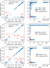 |
Fig. 5 Reliabilities of our best candidate central star matches for confirmed PNe in HASH compared to the reliabilities of the matches for those same PNe published by KB18 (top), S+20 (middle), and GS19 (bottom). The histograms reflect the total counts of reliabilities of matches from previous works, with the top histogram for KB18 also including reliabilities of best matches for all PNe in SH10, including those for which KB18 did not find matches. |
3.1.2 Results
The results of our comparisons are shown in Fig. 5 and Table 1, with individual examples in Fig. 6. There are two considerations: whether the best match found by our method is the same as that found by a previous work, and the reliability assigned to that match by our method (and to the previous work’s match, if different).
Following the thresholds defined earlier, we consider our method to agree with a previous work if it assigned reliability >0.8 to that work’s match, and to have rejected the previous work’s match if it assigns reliability <0.2. Rejections in which our method identified the same best match but assigned it low reliability indicate that our method considered there to be no good candidates (objects on the lower left diagonals of the scatter plots in Fig. 5). These low reliability candidates are excluded from our analysis and our published best matches catalogue. Rejections in which our method found a different best match appear as off-diagonal symbols in the scatter plots in Fig. 5; those cases in which the different best match is plausible (reliability >0.2) count towards disagreements in the histograms in that figure as well as in the counts in Table 1.
We find good agreement overall with KB18, though there is a non-negligible fraction of disagreements (e.g. Fig. 6b) and rejections (e.g. Fig. 6h). Many appear to be due to differences in input catalogue positions; manual spot-checks suggest that the positions in HASH are generally better than those in SIMBAD.
We do believe that any potentially incorrect associations in KB18 are unlikely to substantially change the results of their distance comparisons, because of restrictions on colour and the outlier cuts that they used in their regressions. Indeed, our method matched all of their colour-selected sample (−0.65 < BP – RP < −0.25), and rejectedonly three of their sources with relative parallax errors better than 15% (though these do not correspond to the outliers noted in their regression). Those rejected sources were those for K 3-55 (PN G069.7+00.0), for which we found nogood match, and Hen 2-114 (PN G318.3-02.0) and Sh 2-71 (PN G035.9-01.1), for which we found different matches. In the latter two cases, the parallaxes of our matches had larger uncertainties and would not have been included in the KB18 regression had they been matched. However, while there was tension between the parallaxes of the sources in KB18 and the statistical distances to those PNe, with our matches that is no longer the case.
We also find many matches that were missed by KB18, matching 38% of the PNe in SH10 and not already in KB18. This is slightly lower than our overall rate of 44%. These new matches from SH10 that are not in KB18 tend to lack secure colour information, either missing BP – RP colours altogether or having a high BP/RP excess factor due to nebular contamination or crowded fields8 . Some are also for compact PNe where the central star is likely not visible through the nebula9 .
The catalogues of GS19 and S+20 have lower coincidence with ours than KB18, perhaps because they relied on purely positional cross-matching. As with KB18 there is a mix of rejected sources and disagreements as to which source is the best candidate.
Many of the sources in S+20 that disagree with ours have coordinates matching those of K03. Some of the central star positions in K03 appear to be those of field stars, sufficiently central to find the PN but otherwise unrelated10 . The single band imagery used would have made it difficult to distinguish true central stars based on colour. Likewise, without narrowband imagery, stellar-like PNe are prone to confusion with stellar sources. The Hα imagery in more recent surveys that the HASH positions are based on results in fewer misidentifications.
Even where input catalogue positions agree, our positional matching is more conservative than previous works (e.g. Fig. 6i). Most sources further than 1′′ are rejected by our method unless they are particularly blue (Fig. 4, upper right). This contrasts with the 2′′ and 5′′ search radii used by GS19. Spurious matches in both of these works tend to have lower distances than the PNe to which they are incorrectly associated, and to have relatively good parallax uncertainties that increase their chances of passing parallax quality cuts and making their way into scientific analysis. In the course of their Hβ surface brightness distance scale calibration, S+20 found several objects in their sample with small physical radii (derived from the Gaia parallaxes of their matches) that were noticeably poor fits to the overall trend. They termed these “low ionised mass” PNe, and excluded them from much of their analysis. We believe that most of this population is in fact explained by these PNe incorrectly being matched to nearby field stars, causing their distances to be underestimated. This in turn led to the physical radii being underestimated, as well as their ionised masses. Indeed, among the 18 objects marked as “low ionised mass” in S+20’s Fig. 3, 12 were rejected in our matching.
In general, even mismatches that do not result in obvious outliers can affect results. For example, they can skew distance scale calibrations or cause an overestimate of the local PN population.
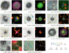 |
Fig. 6 Paired quotient (r′ – Hα) and colour (u′, g′ , r′) images from VPHAS+ of selected PNe centred on their coordinates from HASH. North is up and east is to the left. The coloured markers overlayed on the quotient images show Gaia detections with colour corresponding to BP – RP as shown in the legend and shapes indicating matches from this and previous works. The broadband colour images (with colours derived following Lupton et al. 2004) are useful for comparison as they better capture the range of stellar colours and highlight blue central stars. |
Comparison counts with previous works.
3.1.3 Individual objects
Illustrative examples of individual objects are shown in Fig. 6. They have been selected to show different match scenarios and disagreements with previous works11. For simplicity we limit these examples to ones with imagery from VPHAS+, which restricts the examples to PNe visible from the south and located near the galactic plane. The VPHAS+ survey is particularly useful in that it includes the u′ band, whichcan more clearly separate hot CSPNe from main sequence stars. It is important to note that these images are for illustrative purposes only, and that our method relied solely on the photometry and positions from Gaia.
Some CSPNe have blue Gaia colours, though many are missed by previous works relying purely on positional cross-matching:
-
M 1-18. This is a straightforward case with a blue centrally located star. The PN is in the SH10 catalogue but its central star was missed by KB18 and other previous works, so it does not appear in the scatter plots of Fig. 5.
PB 1.We believe the redder, less central star selected by KB18 to be a misidentification.
IC 1295. The blue central star is 2.1′′ from the HASH position and is correctly selected by our method despite its separation. S+20 has selected a source with no Gaia colour that is 3.2′′ away from the HASH position.
SB 38.The blue central star is 0.5′′ from the HASH position. GS19 has selected a source 2′′ away that is nearly 3 magnitudes brighter and appears to correspond to the PN’s position in K03.
Other stars do not appear blue in Gaia, for various reasons:
-
Hen 2-39. The central star of this PN is dominated by a binary companion (Miszalski et al. 2013) and appears red in Gaia. Our method matched it based on its very central position, 0.2′′ from that in HASH.
H 2-41. The central star of this PN has no Gaia colour and was matched by our method, albeit with low certainty, purely based on its position 0.6′′ from that in HASH. It is only through comparison with the VPHAS+ imagery that it can be seen to be the correct match, rather than the redder off-centre star selected by S+20.
Colour is less indicative for compact or stellar-like PNe, so accurate catalogue positions are particularly important:
-
M 1-38. The central star of this PN appears to be obscured by the nebula itself, but there is a Gaia detection.
-
K 3-13. No central star or bright spot is visible, and KB18’s match is rejected by our method as too far away.
Colour is also important for disambiguation when separations are large or there are multiple possible options:
-
LoTr 3. There appears to be no central star detection (nor is one visible in the imagery), and the purely positional cross-matches of GS19 and S+20 have selected a nearby source whose colour and absolute magnitude are consistent with a main sequence star.
NGC 2899. The stars selected by GS19 and by our method both appear to be incorrect. The true central star is a fainter blue star visible towards the south-west, but it lacks a Gaia colour and is therefore challenging to identify from the Gaia data alone.
SB 39. As with NGC 2899, the true central star of this PN is not one of the sources nearest to its centre. However its blue colour in Gaia has allowed our method to correctly identify it. It is not included in previous works, so it does not appear in the scatter plots of Fig. 5.
3.2 Catalogue
Our full best matches catalogue (Table B.1) is available at the CDS, containing the highest reliability matches from Gaia DR2 for all true, likely, and possible PNe in HASH, for which the reliability is at least 0.2 (our threshold for a possible match). The catalogue contains, for each PN, the PN G identifier and name, the Gaia DR2 source ID for the single best match for that PN, and the reliability of that match determined by our algorithm. The reliability should be used as a filter to limit analysis to high confidence matches (e.g. reliability >0.8), with the particular threshold being dependent on the application. In addition the table contains selected columns from the Gaia catalogue and from HASH are that are particularly relevant to the matching and to the science results presented in this work. From Gaia we include the position, colour, magnitude, and parallax of the best matching sources, as well as a derived quantity indicating the astrometric goodness of fit. From HASH we include PN positions and radii, and their confirmation status (confirmed, likely, or possible PN). We also include the separation between the PN and Gaia source positions. Finally, for convenience, we include cross-match flags with the previous works mentioned in this section and the list of PN binaries in Fig. 9.
It is important to treat the matches that we provide probabilistically and appropriately in context. There is a great deal of additional information not used in our matching, such as source magnitude and parallax, that can help to disambiguate uncertain cases. For example, if a candidate source has a precise parallax that strongly disagrees with other reliable distance measures or leads to an implausible physical nebula size, that adds weight to the source in fact being coincidental, especially in the absence of strong evidence from other non-positional features such as colour. These caveats are, of course, not unique to our work, though ours is the first to attempt to quantify the uncertainties involved.
4 Applications
The subset of matched Gaia sources with parallaxes offers a significant increase in the number of primary galactic PN distance measurements, even with additional restrictions on parallax uncertainties or other quality indicators (e.g. Fig. 10). We present some indicative results using these parallaxes to characterise PN physical properties and revisit the statistical distance scale of FPB16.
Throughout this section we use ω to indicate parallax. This is consistent with the notation in previous works based on Gaia data (e.g. Lindegren et al. 2016).
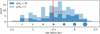 |
Fig. 7 Histogram of PN physical radii derived from Gaia parallaxes of matched CSPNe with various relative parallax error cutoffs. For comparison with Fig. 8, circle sizes used to denote physical radii are shown in the lower panel. |
4.1 Physical parameters
Accurate distance measurements enable us to transform angular sizes of PNe to physical radii. Combined with kinematical assumptions physical radii can determine the age of the nebula. Moreover we can also determine the luminosity of the central star, which is also related to its age and thereby its position on the evolutionary track between AGB and white dwarf stages.
The distribution of physical radii is shown in Fig. 7 for PNe whose matched central stars have a relative parallax error better than 20%. With these errors parallax inversion produces relatively well-behaved distance estimations (Bailer-Jones 2015), which we deem acceptable for the indicative results that we present, particularly since we are not making overall population characterisations that would be biased by this sort of selection.
For central stars in Gaia with both full astrometric solutions and full photometry, we combine the Gaia G band magnitude and the distance estimate from the parallax to estimate the absolute magnitude, and plot this against BP – RP colour in an observational Hertzsprung–Russell diagram (HRD), following Gaia Collaboration (2018a) (Fig. 8). Even without correction for reddening and extinction, most of our matches occupy an otherwise sparsely populated region of the HRD, bluer than the main sequence and giant branch but also brighter than white dwarfs.
4.1.1 Theoretical tracks
Comparison to theoretical tracks requires mapping between the physical stellar parameters of effective temperature Teff and bolometric luminosity L and the observed Gaia BP – RP colours and G magnitude. The goal of the Gaia astrophysical parameters inference system (Apsis) is to perform this mapping starting from Gaia observations, deriving it based on machine learning techniques (Bailer-Jones et al. 2013). Apsis will ultimately use the Gaia spectrophotometry and account for reddening and extinction as well. In Gaia DR2, temperatures are available for less than 10% of sources, and luminosities for less than half of those. Moreover, because of the limited temperature range of the training data, the Teff values that the model does produce do not go above 10 000 K (Andrae et al. 2018), making them unhelpful for the much higher temperature range expected for CSPNe.
Instead we perform the mapping in the opposite direction, transforming physical parameters into observables. Such transformations were provided pre-launch for main sequence and giant stars by Jordi et al. (2010), and for white dwarfs in a followup paper by Carrasco et al. (2014). Though the latter transformations cover higher surface gravities and extend the range of effective temperatures, the two together still miss most of the CSPN evolutionary tracks that we wish to cover. Fortunately, the transformation for higher temperature objects such as CSPNe is largely independent of metallicity and surface gravity. We use the revised BP and RP passbands from Evans et al. (2018) and assume blackbody spectral energy distributions (SEDs) to generate expected BP – RP colours. We find that these are bluer than expected from the pre-launch papers and speculate that this is due to higher sensitivity than expected at the shortest wavelengths. The bluer tracks are also a better fit for the observed data. For transforming luminosity into absolute Gaia G magnitude we adopt the bolometric corrections from Carrasco et al. (2014) for a surface gravity (log g) of 7, fitting a cubic spline to extrapolate to the highest temperature regime. The G passband more closely matches the nominal, pre-launch passband, so we do not expect these calculations to change significantly.
Using these transformations, we plot a selection of tracks from Miller Bertolami (2016) for solar metallicity (Z0 = 0.01, versus 0.0134 for the sun) and a range of initial masses. Bolometric corrections change the shape of the tracks from those in the temperature versus luminosity space, with higher temperature objects at the same luminosity having more of their flux at ultraviolet wavelengths outside the Gaia G band. Thus peak temperature occurs at a G absolute magnitude of around 5, with higher temperatures appearing fainter.
The theoretical tracks are relatively close to each other in the BP – RP colour space, as the Gaia BP – RP colours are not highly sensitive to temperature in the high temperature regime occupied by CSPNe. Between this and the degeneracy between temperature and reddening, we are not able to constrain initial masses and ages from the Gaia DR2 photometry alone (this degeneracy and the insufficiency of Gaia photometry alone is noted for white dwarfs in Gentile Fusillo et al. 2019). Such determinations require additional photometry or spectroscopy to better constrain and disentangle reddening and temperature. The Gaia estimated distances combined with dust maps may prove useful in this regard.
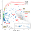 |
Fig. 8 PN central stars plotted on an observational HR diagram, with the circular markers scaled according to the physical radii of the PNe as in Fig. 7. Filled circles indicate objects with the lowest uncertainties. Individual PNe referenced in the text are coloured red rather than blue and accompanied by the PN name. Red lines represent CSPN tracks from Miller Bertolami (2016) for solar metallicity and various initial masses, with the green portions of the line denoting time since leaving the AGB of between 1000 and 20 000 yr, indicative of the sorts of timescales during which a PN could be visible. The peak temperatures of these tracks, through which the stars evolve relatively quickly, are located at an absolute Gaia magnitude around 5 (see text for details). In the background, the grey points are the other sources that were loaded in the 60′′ search windows, with σω∕ω < 10%. They trace out the main sequence (MS) and giant branch. The beginning of the AGB is also labelled, with its position taken from Gaia Collaboration (2018a). White dwarfs are shown separately, as they are too rare to appear otherwise, with the grey contours in the lower left representing the 10, 30, and 50% density contours of the observed high confidence white dwarf candidates from Gentile Fusillo et al. (2019), where the same quality cuts have been made as for the background points. |
4.1.2 Discussion
We find that most of our matched central star colours and absolute magnitudes are well explained by the theoretical tracks plus reddening effects. Additionally, the physical sizes of the nebulae are consistent with the evolutionary direction of their central stars, in that younger and therefore brighter central stars have less evolved nebulae.
Some CSPNe do show inconsistencies; that is those with relatively red BP – RP colours whose de-reddened projection onto the theoretical tracks is a poor fit. We focus on those with that are for resolved nebulae (so that the Gaia detection is of the central star rather than the nebula itself) and have low BP/RP excess factors (indicating well-behaved photometry; colour uncertainty from high excess factors likely dominates any flux uncertainties).
One explanation is that these are binary systems where the light from actual progenitor of the PN is dominated by a main sequence companion. A few examples that we checked are LoTr 5 (PN G339.9+88.4) and BE UMa / LTNF 1 (PN G144.8+65.8), which have the largest absolute latitudes of the red sample, meaning that their colours are less likely to be reddened. Both of these are in fact known binary systems (Jones et al. 2017; Ferguson et al. 1999 respectively), as is NGC 1514 (PN G165.5-15.2) in the first reference. WeBo 1 (PN G135.6+01.0), the reddest star in the sample with a large BP – RP value of 1.9, is also a binary (Bond et al. 2003), while the second reddest star, the central star of PMR 1 (PN G272.8+01.0) with BP – RP equal to 1.7, is noted in the literature to simply be heavily reddened (Morgan et al. 2001). These are highlighted in Figs. 8 and 9 along with the other individual PNe mentioned in this section.
One star that does appear inconsistent with the nebula size versus absolute magnitude trend is NGC 2438 (PN G231.8+04.1). The veracity of its identification as the central star is confirmed by its colour, but its parallax measurement places it around 422 pc away, with less than 10% error, which is inconsistent with other distance determinations for the PN. The statistical scale of FPB16 estimates the PN’s distance to be 1.54 ± 0.44 kpc, consistent with an even further away estimate from central star modelling that was used as part of that paper’s calibration. We believe that the parallax errors in this case may not be well-behaved, supported by the source having high astrometric excess noise (and renormalised unit weight error (RUWE) = 2.39). Assuming NGC 2438 to be further away removes tensions, leading to a larger physical nebula size and a brighter central star.
The HRD suggests the possibility of further refinement of the matching itself based on parallaxes, with the derived absolute magnitudes disambiguating between possibly reddened CSPNe and main sequence stars, and the derived distances allowing for the calculation of a physical radius which can then be checked for compatibility with other knowledge about the PN. Stars that do lie on the main sequence and have plausible parallaxes merit further investigation as possible mismatches, binaries, or reddened single central stars.
An example of an implausible match is that of the “likely” PN Abell 19 (PN G200.7 + 08.4). The centrally located star is nearby, at around 250 pc away, with small parallax uncertainties and a colour and magnitude that place it neatly on the main sequence (Fig. 8). While the colour could be explained by reddening, significant reddening is unlikely given the star’s relatively close proximity; this is confirmed by its low estimated reddening in FPB16 (Fig. 9). It is also unlikely to be a binary companion, because the PN physical radius of 0.05 pc (log physical radius of −1.3) resulting from its parallax is smaller than almost all of the PNe in our sample (Fig. 7) and consistent with a very young PN, which would then have a much brighter central star and nebula. Thus we can conclude that this candidate is more likely to be a nearby field star.
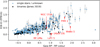 |
Fig. 9 Reddening values E(B–V) and their given uncertainties taken from FPB16’s statistical distance compilation12 plotted against Gaia BP – RP colours for all matches with reliability > 0.8 (not limited by parallax uncertainties). Known and suspected binary systems taken from the compilation of David Jones13 are highlighted as black squares14. Objects lying below the trend (objects appearing red in Gaia with low reddening) could be binary systems or have significant reddening internal to the nebula, or could have dubious identification. Relevant individual objects mentioned in the text are shown in red. |
4.2 Statistical distance scales
The parallaxes from Gaia also offer an opportunity to evaluate and ultimately refine statistical distance scales. We focus on the Hα surface brightness to physical radius relation from FPB16, which was calibrated based on distances to galactic and extragalactic PNe derived from a variety of primary techniques, including parallaxes from the HST and USNO but not from Gaia.
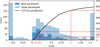 |
Fig. 10 Relative parallax errors σω∕ω for the bestmatches (reliability >0.8) sub-sample of confirmed PNe, along with the cumulative counts below various reliability thresholds for positive parallaxes (in black). The bins at either end represent the counts or matches with σω ∕ω falling outside of the range (−0.5, 1.5). Within the sample, those parallaxes meeting more stringent criteria (reliability > 0.98, σω < 0.2 mas, RUWE < 1.4, visibility_periods_used > 8) are indicated by the darker shaded area of the histogram. This subset is used for the Frew et al. (2016) distance comparisons. |
4.2.1 Distance ratios
The caveats present in using parallaxes to estimate distances are well known (Luri et al. 2018); in particular naive parallax inversion does not produce a statistically sound distance estimate for any reasonable choice of prior, and any attempt to limit an analysis to parallaxes with relative error σω∕ω below some threshold (as was done in the previous section), or even to positive parallaxes (as inverting negative parallaxes is unphysical) introduces biases. We can avoid these caveats by staying in the space of parallaxes, where the errors are well-behaved.
The notion of distance ratios described in Smith (2015) avoids these caveats by sidestepping parallax inversion entirely and taking the product over objects of measured parallaxes ω′ and estimated statistical distances  to form a distance ratio
 (4)
(4)
with associated uncertainty
 (5)
(5)
where dS is the true distance d multiplied by the distance ratio RS and σS is the standard error on the statistical distance. The distance ratio can be used to measure both errors in the intercept of a statistical relation (through deviations in the mean distance ratio away from unity) and in its slope (through correlations between the distance ratio and the estimated physical radius or statistical distance).
4.2.2 Methods
We consider the set of 1024 confirmed PNe for which FPB16 published statistical distances. Our method finds likely central star matches for 636 of them, though we further whittle down the selection as follows.
To limit the effect of poorly behaved parallaxes we apply quality cuts similar to those used in Gaia Collaboration (2018a). We require a slightly higher number of observations than the threshold for inclusion into the Gaia data release, that is visibility_periods_used > 8. Additionally we set an upper limit on the renormalised unit weight error (RUWE) of 1.4 as recommended by Lindegren (2018). This is a goodness-of-fit statistic that indicates how well the Gaia astrometric solution matches that expected for a single star (Lindegren et al. 2018). Finally, we apply a cut on the absolute uncertainty of the parallax itself, requiring σω < 0.2 mas.
The aim of these cuts is to reduce the overall uncertainty in the average distance ratio without biasing its value. Thus we choose a cutbased on absolute rather than relative parallax error, which avoids truncation biases. As parallax uncertainty is related to apparent magnitude, any cut based on parallax does bias the selection towards brighter and nearer objects, but that is unavoidable. It is worthwhile to note that there is also a risk that the cut based on RUWE could bias the sample by preferentially eliminating binary systems, though we do not see strong evidence that this is the case.
To avoid the effect of any incorrect matches we also apply a stricter reliability cut of reliability >0.98, which keeps the vast majority of the matches. Altogether the quality cuts leave us with 160 objects out of the 636 objects from FPB16 that we matched.
For many PNe, FPB16 provided multiple distance estimates: one based on a general trend, and one based on a subtrend for PNe that are classified as either optically thick or optically thin. The subtrend relationships have different slopes from each other and lower scatter. The calibrating set in FPB16 was chosen to represent a range of PN properties, and is balanced between optically thin and thick objects. If the subset that we compare is a different mixture, it will deviate from the mean trend even if the distances are correct. We consider this in the following section.
4.2.3 Results
Using the mean trends gives a mean distance ratio of 1.15 ± 0.07 for the 160 objects that passed the quality cuts, while using the subtrends reduces this ratio to 1.03± 0.06 (the uncertainties are calculated via bootstrapping). We note that the matched PNe show a preference for optically thin PNe relative to the mixture of thick and thin PNe that formed the mean trend in FPB16, which could be due to optically thin PNe being more likely to have visible central stars. The subtrend in FPB16 for optically thin PNe has such PNe having lower surface brightnesses for the samephysical radius, which translates to the mean trend overestimating the physical radii for these objects and thus overestimating their distances. This is consistent with the difference in mean distance ratios we see comparing the mean trend and subtrends.
The results using the subtrends are shown in Fig. 11. On average the Gaia parallaxes meeting our quality cuts are consistent with the associated FPB16 statistical distances. This is not surprising given the many extragalactic distances in the set of calibrating distances and the use of parallaxes in the calibration itself, which mean that the distance scale is unlikely to deviate from a true distances by the factors of two that older scales suffered from Smith (2015). There is a slight suggestion of a dependency on physical radius but the uncertainties are too large to draw a meaningful conclusion. Grouping by morphology (lower half of Fig. 11), we find no significant deviations from a mean distance ratio of unity, with round PNe having the largest deviation at 1.15± 0.12.
We seesome notable outliers, objects for which |(RS − 1)∕σS| is large. Only a couple have parallax-derive dist- ances significantly smaller than their statistical ones:
K 1-6. The statistical distances from both the mean trend (1.85 ± 0.53 kpc) and thin trend (1.45 ± 0.27 kpc) for K 1-6 (PNG 107.0 + 21.3) appear to be significant overestimates relative to its central star parallax, which places it within 500 pc. The distance from the thin trend is smaller and thus closer, but its smaller uncertainties make the disagreement more significant. This PN was studied by Frew et al. (2011), who note tensions between different distance estimates for that nebula in terms of its surface brightness and the properties of its binary central stars; they adopt a distance of 1 kpc, halfway between FPB16’s statistical distances and that suggested by the parallax from Gaia. They also note a range of possible distances based on the spectroscopic parallax of the binary central star companion, with the short end of those distances being consistent with the now observed trigonometric parallax.
Abell 28. Similarly to K 1-6, the Gaia parallax for the blue central star of Abell 28 (PNG 158.8+37.1) places it within 500 pc, much closer than its statistical distances of 1.67 ± 0.48 kpc and 1.29 ± 0.25 kpc from the mean and thin trends respectively. The parallax-derived distance places it in the population of “subluminous” PNe noted in Sect. 4.3.4 of FPB16, with Abell 28 then occupying a place in the surface brightness versus physical radius plane near that of RWT 152 (PNG 219.2 + 07.5) (the parallax of the central star of RWT 152 itself is consistent with both the primary and statistical measurements).
On the other end of the scale there are several objects whose parallax-derived distances are significantly larger than their statistical ones (empty symbols below the dashed line in Fig. 11). There is a suggestive excess of elliptical / bipolar objects in this set that would match the trend that FPB16 observe of bipolar objects having higher surface brightnesses, but even comparing the calibrating distances of those objects the Gaia parallaxes shows significant disagreement by up to a factor of two, for example for Hen 2-11 (PN G259.1+00.9), whose parallax of 0.5 mas gives it a 2σ distance range of 1.25–5 kpc from Gaia, outside of the relatively confident 730 pc estimate derived from modelling of its binary star by Jones et al. (2014) that is also used in the calibrations by FPB16. One possibility is that the parallaxes are themselves skewed by binarity, as in Gaia DR2 only single stars are modelled. Also, as the uncertainties in statistical distances are correlated with the statistical distances themselves, statistical distances that are underestimates also have underestimated uncertainties, which in turn means that the uncertainty in the distance ratio is underestimated. This effect is noted by Smith (2015).
 |
Fig. 11 Histograms of distance ratios RS and normalised distance ratios RS∕σS derived from comparison between Gaia parallaxes and statistical distances (using subtrends) from FPB16. Ratios are plottedfor both the higher quality set of parallaxes (see text) and rejected parallaxes for comparison, in dark and light blue respectively. The plot on the left shows the raw distance ratios, with the mean value of 1.03 ± 0.06 for the best quality parallax set. On the right the distance ratios have been re-centred around RS = 1 and divided by their estimated uncertainties σR. Though the distribution of distance ratios is not expected to be Gaussian, a standard normal distribution is over-plotted for comparison. Below is a scatter plot depicting the distance ratios of the best parallax subset against the physical radius derived from the statistical distance. Marker colours and shapes show morphological classifications taken from HASH. Trends in this plot (that is, a correlation between distance ratio and radius) would be indicative of a slope differing from that derived in FPB16. Filled markers have RS within 2.5σS of 1 (dashedline). Outliers are empty markers, with the two outliers specifically mentioned in the text highlighted. The correlation coefficients are 0.18 and 0.08 with and without the outliers respectively. The former is very weakly significant, while the latter is not. |
4.2.4 Discussion
The fraction of outliers would increase significantly if we lowered the reliability threshold of our method and accepted nearest neighbour Gaia sources that we had not considered to be matches. The selection of such mismatches based on distance ratios is biased towards nearby objects, which tend to have lower parallax errors (on account of being brighter) and larger parallaxes that more tightly constrain their distances. Such mismatches will become more noticeable in future data releases as parallax uncertainties tighten, however, even mismatches that are individually consistent within errors will globally skew any calibration or evaluation, making it important to have a robust selection process to begin with. As with the HRD in the previous section, additional data, in this case distance priors based on statistical distances derived from nebula properties, can be used to further refine the matching by placing bounds on reasonable parallaxes.
Ultimately the Gaia parallaxes will offer a new opportunity to calibrate statistical distance scales such as that of FPB16 using galactic PNe and bring the uncertainties closer to the intrinsic scatter of the relationship. Trigonometric parallaxes provide the most direct means of measuring distances, but their properties mean that they require a proper prior on the underlying distances which must be accounted for at the level of the derived relationship rather than for individual distances such as those published in the catalogue by Bailer-Jones et al. (2018). Selection effects may be present as well as certain types of PNe may be more amenable todistance determination from central star parallaxes. Performing such a calibration is beyond the scope of this particular work, but we believe that the uniform matching performance of our automated technique will offer a good basis for such work in the future, in particular with the improved data in the forthcoming Gaia EDR3.
5 Conclusions
We have used a novel application of the likelihood ratio method to automatically match central stars of planetary nebulae in the HASH PN catalogue with sources in Gaia DR2 based on their positions and colours, with a particular focus on accuracy and consistency that contrasts with previous works. Our catalogue of matches includes confidence scores, and is the largest available for Gaia DR2 at the time of writing. We have described a few examples of how this catalogue and the new data offered by Gaia will enable future science, and discussed the importance of accurate matching in achieving these aims. We emphasise that the certainty of the matching itself should be considered holistically in any analysis.
There are opportunities for further refinement of our matches based on additional data. Photometry from other surveys could disambiguate where Gaia colours are lacking, though Gaia itself will improve significantly on this front in the future with the full BP/RP spectrophotometry (low resolution spectra). As noted in the previous section, the candidate central star sources with the best parallaxes can be further evaluated on their plausibility as central stars based on their positions in the HR diagram and whether the resulting distance is compatible with the angular size and surface brightness of the nebula itself. Equally, outliers in these parameter spaces can point to interesting sources and systems for followup and further study, such as binary central stars.
Our automated method makes it possible to easily and quickly update the catalogue based on future Gaia data releases and future PN discoveries. This will enable us to leverage the improved completeness and more precise astrometric measurements in those future data releases to better understand the galactic PN population.
Acknowledgements
We thank the anonymous referee for their comments, which have helped improve this paper. This research has made use of data from the European Space Agency (ESA) mission Gaia (https://www.cosmos.esa.int/gaia), processed by the Gaia Data Processing and Analysis Consortium (DPAC; https://www.cosmos.esa.int/web/gaia/dpac/consortium). Funding for the DPAC has been provided by national institutions, in particular the institutions participating in the Gaia Multilateral Agreement. This research has also made use of the HASH PN database (http:// hashpn.space), of Astropy (http://www.astropy.org), a community-developed core Python package for Astronomy (Astropy Collaboration 2013, 2018), and of “Aladin sky atlas” developed at CDS, Strasbourg Observatory, France. Parts of this research were based on data products from observations made with ESO Telescopes at the La Silla Paranal Observatory under programme ID 177.D-3023, as part of the VST Photometric Hα Survey of the southern Galactic plane and bulge (VPHAS+; www.vphas.eu), as well as data obtained as part of the INT Photometric Hα] Survey of the northern Galactic plane (IPHAS; www.iphas.org) carried out at the Isaac Newton Telescope (INT). The INT is operated on the island of La Palma by the Isaac Newton Group in the Spanish Observatorio del Roque de los Muchachos of the Instituto de Astrofisica de Canarias. All IPHAS data are processed by the Cambridge Astronomical Survey Unit (CASU), at the Institute of Astronomy in Cambridge. This research was supported through the Cancer Research UK grant A24042.
Appendix A Implementation details
The probability densities functions (PDFs) used to calculate the likelihood ratio (Eq. (2)) are estimated from the data themselves. The particular methods and parameters were chosen with the overall aim of producing smooth density ratios with few extrema and to thereby avoid overfitting.
A.1 Colour density ratio estimation
Our goal is to estimate the density in BP – RP colour space of true CSPNe and of non-CSPNe (background sources). We determine our estimates empirically by choosing representative examples of both kinds of sources based on their positions.
The BP and RP fluxes measured by Gaia can be contaminated by light from nearby sources (within a couple of arcseconds), particularly in densely populated or nebulous regions. For well-behaved sources with no contamination, it is expected that the total flux measured in the BP and RP passbands should approximately match that of the G band, which does not have the same possibility of contamination. Deviations from this relation are indicated in the catalogue by a large photometric excess factors, and Evans et al. (2018) suggests using cuts based on this factor to select photometrically well-behaved sources for applications relying on colour information. Rather than ignoring the colours of these high excess factor sources completely with hard cuts, we incorporate the excess factor into our density estimation, treating the source colour space as two-dimensional.
We bin sources by excess excess factor (distance above the locus of well-behaved colours, that is phot_bp_rp_excess_factor− 1.3 × bp_rp2, taken from Evans et al. 2018) with overlapping bins. We compute the density ratio within each bin as a function of BP – RP alone, and then smoothly interpolate to get the density ratio values for excess factors between bin centres (interpolating towards one for high excess, corresponding the colour density ratio of one for sources lacking colours). Thus while the density ratio function has a two-dimensional domain, colour densities are only ever one-dimensional in BP – RP. We thereby hope to treat excess factor as only a quality indicator.
We estimate the density ratios at each BP – RP value within a single bin non-parametrically using kernel density estimation with a Gaussian kernel. Because of the highly varying density, we use a balloon estimator, in which the kernel bandwidth (the standard deviation of the Gaussian in this case) is variable and is inversely proportional to the local density at the sample point. We estimate the local density from the distance to the nth nearest neighbour in BP – RP, so the kernel bandwidth is effectively proportional to distance to the nth nearest neighbour. The bandwidth is clipped to lie within a range of well-behaved values. To avoid artefacts from mismatched kernel widths, the same kernel width is used for both the numerator and denominator of the density ratio, with the kernel chosen based on the numerator density (the density of BP – RP colours for candidate central stars chosen based on distance or nearest neighbour), since there are fewer such sources.
Sources used to estimate the background colour density (either non-nearest neighbour sources in the first iteration or sources with low separation density ratios in the second iteration) are weighted by the inverse of the local spatial source density ρ. The idea of this is that each PN neighbourhood is given equal weighting in the denominator of the colour density ratio estimation (the colour density for background sources). Each PN neighbourhood is by default equally weighted in the estimate for genuine match colours (the numerator), since all neighbourhoods contribute (at most) a single candidate genuine match and are thus weighted equally in that calculation.
A.2 Separation density ratio estimation
The set of sources used to estimate the separation density ratio is those with a colour likelihood ratio > 20 from the initial (nearest neighbour) colour density ratio estimation. We apply a cutoff on the separation s to these sources, requiring that s < rPN + 2′′ where rPN is the PN radius in arcseconds, with the addition of 2′′ reflecting our expectation that the relative positional uncertainty is greater for smaller PNe. There are n Gaia sources that met our cutoff, having separations si, i = 1…n. These sources are associated with confirmed (PNstat = T in HASH) PNe with radii <600′′ (including unresolved PNe with no size information in HASH, which we treat for the purposes of binning as having radii of 0.25′′).
As noted in Sect. 2.2.2 and Fig. 3, the distribution of separations s does not match well with a single Rayleigh distribution, unsurprising given the multiple sources of positional uncertainty. However adopting a fully non-parametric approach does not work as well as it did for the colour density in the previous section.
The PDF of a Rayleigh distribution is
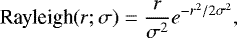 (A.1)
(A.1)
which has the convenient property that the r term cancelswith the r in the PDF for a constant density of background sources, that is 2πrρ, giving a likelihood ratio that levels off at a finite value as the separation approaches 0. This reflects the fact that while finding a background source with a very small separation is highly unlikely, so is finding a true counterpart source.
To preserve these properties we form our distribution by mixing n Rayleigh distributions
 (A.2)
(A.2)
with parameters σi each corresponding to the maximum likelihood estimates (MLEs) from a single separation si , that is  . This mixture captures the behaviour of the empirical distribution while ensuring that the resulting density ratio is smooth, strictly decreasing, and well-behaved near zero.
Another advantage of this mixture approach is that the mixture can be reweighted to fit different PN sizes, reflecting the expected dependence in positional uncertainty on the size of the PN. Rather than identical weights wi = 1∕n, we choose mixture weights for a PN with radius rPN as
 (A.3)
(A.3)
scaled so that ∑iwi = 1. We consider log radii as the logarithm is scale invariant, and choose a standard deviation σ =0.5 so that most of the influence comes from PN with radii  within a factor of two of the given PN radius.
A.3 Justification of nearest neighbour approximation
We form our initial estimate of the colour density ratio by splitting our candidate set into nearest and non-nearest neighbours, and use the candidate points with the highest colour density ratio as a kind of initial training set for learning the positional uncertainties. This density estimation (and indeed the second iteration based on position) is contaminated in both directions, with many background sources in the nearest neighbour set (standing in for the CSPNe set) and some true CSPNe in the non-nearest neighbour set (standing in for the background distribution).
The effect of this contamination is to push the density ratio towards one (the density ratio becomes one in the limit where the two distributions contain the same proportions of true CSPNe and background sources). We can still learn useful and valid information from the colour provided that true CSPNe make up a larger proportion of the nearest neighbour set than they do of the non-nearest neighbour set, which we expect will be the case as the non-nearest neighbour set is so much larger to begin with.
References
- Andrae, R., Fouesneau, M., Creevey, O., et al. 2018, A&A, 616, A8 [NASA ADS] [CrossRef] [EDP Sciences] [Google Scholar]
- Astropy Collaboration (Robitaille, T. P., et al.) 2013, A&A, 558, A33 [NASA ADS] [CrossRef] [EDP Sciences] [Google Scholar]
- Astropy Collaboration (Price-Whelan, A. M., et al.) 2018, AJ, 156, 123 [Google Scholar]
- Bailer-Jones, C. A. L. 2015, PASP, 127, 994 [NASA ADS] [CrossRef] [Google Scholar]
- Bailer-Jones, C. A. L., Andrae, R., Arcay, B., et al. 2013, A&A, 559, A74 [NASA ADS] [CrossRef] [EDP Sciences] [Google Scholar]
- Bailer-Jones, C. A. L., Rybizki, J., Fouesneau, M., Mantelet, G., & Andrae, R. 2018, AJ, 156, 58 [NASA ADS] [CrossRef] [Google Scholar]
- Benedict, G. F., McArthur, B. E., Napiwotzki, R., et al. 2009, AJ, 138, 1969 [NASA ADS] [CrossRef] [Google Scholar]
- Blum, A., & Mitchell, T. 1998, in Proceedings of the Eleventh Annual Conference on Computational Learning Theory, COLT’ 98 (New York, NY, USA: ACM), 92–100 [CrossRef] [Google Scholar]
- Bond, H. E., Pollacco, D. L., & Webbink, R. F. 2003, AJ, 125, 260 [NASA ADS] [CrossRef] [Google Scholar]
- Carrasco, J. M., Catalán, S., Jordi, C., et al. 2014, A&A, 565, A11 [NASA ADS] [CrossRef] [EDP Sciences] [Google Scholar]
- Ciardullo, R. 2012, Ap&SS, 341, 151 [NASA ADS] [CrossRef] [Google Scholar]
- Drew, J. E., Gonzalez-Solares, E., Greimel, R., et al. 2014, MNRAS, 440, 2036 [NASA ADS] [CrossRef] [Google Scholar]
- Evans, D. W., Riello, M., De Angeli, F., et al. 2018, A&A, 616, A4 [NASA ADS] [CrossRef] [EDP Sciences] [Google Scholar]
- Ferguson, D. H., Liebert, J., Haas, S., Napiwotzki, R., & James, T. A. 1999, ApJ, 518, 866 [NASA ADS] [CrossRef] [Google Scholar]
- Frew, D., & Parker, Q. 2010, PASA, 27, 129 [NASA ADS] [CrossRef] [Google Scholar]
- Frew, D. J., Stanger, J., Fitzgerald, M., et al. 2011, PASA, 28, 83 [NASA ADS] [CrossRef] [Google Scholar]
- Frew, D. J., Parker, Q. A., & Bojičić, I. S. 2016, MNRAS, 455, 1459 [NASA ADS] [CrossRef] [Google Scholar]
- Gaia Collaboration (Brown, A. G. A., et al.) 2016a, A&A, 595, A2 [NASA ADS] [CrossRef] [EDP Sciences] [Google Scholar]
- Gaia Collaboration (Prusti, T., et al.) 2016b, A&A, 595, A1 [NASA ADS] [CrossRef] [EDP Sciences] [Google Scholar]
- Gaia Collaboration (Babusiaux, C., et al.) 2018a, A&A, 616, A10 [NASA ADS] [CrossRef] [EDP Sciences] [Google Scholar]
- Gaia Collaboration (Brown, A. G. A., et al.) 2018b, A&A, 616, A1 [NASA ADS] [CrossRef] [EDP Sciences] [Google Scholar]
- Gentile Fusillo, N. P., Tremblay, P.-E., Gänsicke, B. T., et al. 2019, MNRAS, 482, 4570 [NASA ADS] [CrossRef] [Google Scholar]
- González-Santamaría, I., Manteiga, M., Manchado, A., Ulla, A., & Dafonte, C. 2019, A&A, 630, A150 [NASA ADS] [CrossRef] [EDP Sciences] [Google Scholar]
- Harris, H. C., Dahn, C. C., Canzian, B., et al. 2007, AJ, 133, 631 [NASA ADS] [CrossRef] [Google Scholar]
- Herwig, F. 2005, ARA&A, 43, 435 [NASA ADS] [CrossRef] [Google Scholar]
- Hillwig, T. C., Margheim, S. J., De Marco, O., & Frew, D. 2013, AAS Meeting Abstracts, 221, 249.09 [Google Scholar]
- Johnson, J. A. 2019, Science, 363, 474 [NASA ADS] [CrossRef] [EDP Sciences] [Google Scholar]
- Jones, D., & Boffin, H. M. J. 2017, Nat. Astron., 1, 0117 [CrossRef] [Google Scholar]
- Jones, D., Boffin, H. M. J., Miszalski, B., et al. 2014, A&A, 562, A89 [NASA ADS] [CrossRef] [EDP Sciences] [Google Scholar]
- Jones, D., Van Winckel, H., Aller, A., Exter, K., & De Marco, O. 2017, A&A, 600, L9 [NASA ADS] [CrossRef] [EDP Sciences] [Google Scholar]
- Jordi, C., Gebran, M., Carrasco, J. M., et al. 2010, A&A, 523, A48 [NASA ADS] [CrossRef] [EDP Sciences] [Google Scholar]
- Karakas, A. I., & Lattanzio, J. C. 2014, PASA, 31, e030 [NASA ADS] [CrossRef] [Google Scholar]
- Kerber, F., Mignani, R. P., Guglielmetti, F., & Wicenec, A. 2003, A&A, 408, 1029 [NASA ADS] [CrossRef] [EDP Sciences] [Google Scholar]
- Kimeswenger, S., & Barría, D. 2018, A&A, 616, L2 [NASA ADS] [CrossRef] [EDP Sciences] [Google Scholar]
- Kwitter, K. B., Méndez, R. H., Peña, M., et al. 2014, Rev. Mex. Astron. Astrofis., 50, 203 [NASA ADS] [Google Scholar]
- Lindegren, L. 2018, GAIA-C3-TN-LU-LL-124 [Google Scholar]
- Lindegren, L., Lammers, U., Bastian, U., et al. 2016, A&A, 595, A4 [NASA ADS] [CrossRef] [EDP Sciences] [Google Scholar]
- Lindegren, L., Hernández, J., Bombrun, A., et al. 2018, A&A, 616, A2 [NASA ADS] [CrossRef] [EDP Sciences] [Google Scholar]
- Lupton, R., Blanton, M. R., Fekete, G., et al. 2004, PASP, 116, 133 [NASA ADS] [CrossRef] [Google Scholar]
- Luri, X., Brown, A. G. A., Sarro, L. M., et al. 2018, A&A, 616, A9 [NASA ADS] [CrossRef] [EDP Sciences] [Google Scholar]
- Marrese, P. M., Marinoni, S., Fabrizio, M., & Giuffrida, G. 2017, A&A, 607, A105 [NASA ADS] [CrossRef] [EDP Sciences] [Google Scholar]
- Marrese, P. M., Marinoni, S., Fabrizio, M., & Altavilla, G. 2019, A&A, 621, A144 [NASA ADS] [CrossRef] [EDP Sciences] [Google Scholar]
- Miller Bertolami, M. M. 2016, A&A, 588, A25 [NASA ADS] [CrossRef] [EDP Sciences] [Google Scholar]
- Miszalski, B., Parker, Q. A., Acker, A., et al. 2008, MNRAS, 384, 525 [NASA ADS] [CrossRef] [Google Scholar]
- Miszalski, B., Boffin, H. M. J., Jones, D., et al. 2013, MNRAS, 436, 3068 [NASA ADS] [CrossRef] [Google Scholar]
- Moe, M., & De Marco, O. 2006, ApJ, 650, 916 [NASA ADS] [CrossRef] [Google Scholar]
- Morgan, D. H., Parker, Q. A., & Russeil, D. 2001, MNRAS, 322, 877 [NASA ADS] [CrossRef] [Google Scholar]
- Parker, Q. A.,& Frew, D. J. 2011, in Asymmetric Planetary Nebulae 5 Conference, 1 [Google Scholar]
- Parker, Q. A., Acker, A., Frew, D. J., et al. 2006, MNRAS, 373, 79 [NASA ADS] [CrossRef] [Google Scholar]
- Parker, Q. A., Bojičić, I. S., & Frew, D. J. 2016, J. Phys, Conf. Ser., 728, 032008 [NASA ADS] [CrossRef] [Google Scholar]
- Salvato, M., Buchner, J., Budavári, T., et al. 2018, MNRAS, 473, 4937 [NASA ADS] [CrossRef] [Google Scholar]
- Schönberner, D., Balick, B., & Jacob, R. 2018, A&A, 609, A126 [NASA ADS] [CrossRef] [EDP Sciences] [Google Scholar]
- Smith, H. 2015, MNRAS, 449, 2980 [NASA ADS] [CrossRef] [Google Scholar]
- Stanghellini, L., & Haywood, M. 2010, ApJ, 714, 1096 [NASA ADS] [CrossRef] [Google Scholar]
- Stanghellini, L., Bucciarelli, B., Lattanzi, M. G., & Morbidelli, R. 2017, New Astron., 57, 6 [CrossRef] [Google Scholar]
- Stanghellini, L., Bucciarelli, B., Lattanzi, M. G., & Morbidelli, R. 2020, ApJ, 889, 21 [Google Scholar]
- Sutherland, W., & Saunders, W. 1992, MNRAS, 259, 413 [NASA ADS] [CrossRef] [Google Scholar]
- Weidmann, W. A., & Gamen, R. 2011, A&A, 526, A6 [NASA ADS] [CrossRef] [EDP Sciences] [Google Scholar]
The version of the likelihood ratio in Eq. (1) is related to the figure of merit used in the Gaia cross-matches with external catalogues (Marrese et al. 2017, 2019).
Otherwise we could have iteratively updated Q and recalculated the reliabilities until they converged. Indeed, the 415 likely and 663 possible PNe have mean reliabilities of 0.45 and 0.34 respectively, indicating a lower success rates for these unconfirmed PNe and also that the chosen Q value of 0.5 is thus inconsistent for them. The relationship between PN status and central star matching success is expected given that a clearly visible central star contributes towards confirming a nebula’s PN status.
We do note that our method failed to find high reliability matches for 20% of the 412 PNe in the Weidmann & Gamen (2011) catalogue listed as confirmed PNe in HASH, which provides some idea of the completeness of Gaia DR2.
Reddening for PMR 1 is taken from Morgan et al. (2001) as it is missing from FPB16. It is missing error bars because there was no uncertainty published for the estimate.
http://www.drdjones.net/bcspn/, as of March 11, 2019.
PHR J1510-6754 (PN G315.4-08.4) is also included as a binary as noted by Hillwig et al. (2013); it is not included in Jones’ list but the reference was found incidentally in a cursory literature search for objects lying below the trend.
All Tables
All Figures
|
Fig. 1 Outline of the steps used in the matching process. |
| In the text | |
|
Fig. 2 Histogram of BP – RP colours for three different sets of Gaia sources covering both iterations of the colour density ratio computation. The grey histogram shows the distribution of colours of background sources, which does not change visibly between iterations. The initial colour distribution derived from nearest neighbouring sources is indicated by the red dashed line. The colour distribution of the final selection based on separation is indicated in blue. Lower panel: density ratio in colour space, also for both iterations, with the final density ratio indicated by the black line, and the initial ratio derived from nearest versus non-nearest neighbours shown by the dashed red line. All densities are for sources with a well-behaved BP/RP excess factor (indicating reliable colour measurements). |
| In the text | |
|
Fig. 3 Histogram of the separations of the “high-confidence” sources (selected by colour) from their PN centres, along with, for comparison, a Rayleigh distribution with a similar mode in red, and a uniform density of background sources in grey. Lower panel: separation density ratio resulting from the derived mixture of Rayleigh distributions compared to that from the single Rayleigh distribution in the upper panel. In practice the mixture is re-weighted depending on the radius of the PN. |
| In the text | |
|
Fig. 4 Matching results for confirmed PNe in HASH. The histogram on the upper left shows the reliabilities of highest ranked candidate central stars for each PN. Over-plotted is the mirrored cumulative distribution function (CDF) of that distribution, with the cutoffs and counts for best and potential matches highlighted. The two scatter plots show the distribution of the matches in colour/separation space and in galactic coordinates, with blue circles being likely matches, grey circles being possible matches, and red circles being rejected sources. Larger circles correspond to PN with larger angular sizes. |
| In the text | |
|
Fig. 5 Reliabilities of our best candidate central star matches for confirmed PNe in HASH compared to the reliabilities of the matches for those same PNe published by KB18 (top), S+20 (middle), and GS19 (bottom). The histograms reflect the total counts of reliabilities of matches from previous works, with the top histogram for KB18 also including reliabilities of best matches for all PNe in SH10, including those for which KB18 did not find matches. |
| In the text | |
|
Fig. 6 Paired quotient (r′ – Hα) and colour (u′, g′ , r′) images from VPHAS+ of selected PNe centred on their coordinates from HASH. North is up and east is to the left. The coloured markers overlayed on the quotient images show Gaia detections with colour corresponding to BP – RP as shown in the legend and shapes indicating matches from this and previous works. The broadband colour images (with colours derived following Lupton et al. 2004) are useful for comparison as they better capture the range of stellar colours and highlight blue central stars. |
| In the text | |
|
Fig. 7 Histogram of PN physical radii derived from Gaia parallaxes of matched CSPNe with various relative parallax error cutoffs. For comparison with Fig. 8, circle sizes used to denote physical radii are shown in the lower panel. |
| In the text | |
|
Fig. 8 PN central stars plotted on an observational HR diagram, with the circular markers scaled according to the physical radii of the PNe as in Fig. 7. Filled circles indicate objects with the lowest uncertainties. Individual PNe referenced in the text are coloured red rather than blue and accompanied by the PN name. Red lines represent CSPN tracks from Miller Bertolami (2016) for solar metallicity and various initial masses, with the green portions of the line denoting time since leaving the AGB of between 1000 and 20 000 yr, indicative of the sorts of timescales during which a PN could be visible. The peak temperatures of these tracks, through which the stars evolve relatively quickly, are located at an absolute Gaia magnitude around 5 (see text for details). In the background, the grey points are the other sources that were loaded in the 60′′ search windows, with σω∕ω < 10%. They trace out the main sequence (MS) and giant branch. The beginning of the AGB is also labelled, with its position taken from Gaia Collaboration (2018a). White dwarfs are shown separately, as they are too rare to appear otherwise, with the grey contours in the lower left representing the 10, 30, and 50% density contours of the observed high confidence white dwarf candidates from Gentile Fusillo et al. (2019), where the same quality cuts have been made as for the background points. |
| In the text | |
|
Fig. 9 Reddening values E(B–V) and their given uncertainties taken from FPB16’s statistical distance compilation12 plotted against Gaia BP – RP colours for all matches with reliability > 0.8 (not limited by parallax uncertainties). Known and suspected binary systems taken from the compilation of David Jones13 are highlighted as black squares14. Objects lying below the trend (objects appearing red in Gaia with low reddening) could be binary systems or have significant reddening internal to the nebula, or could have dubious identification. Relevant individual objects mentioned in the text are shown in red. |
| In the text | |
|
Fig. 10 Relative parallax errors σω∕ω for the bestmatches (reliability >0.8) sub-sample of confirmed PNe, along with the cumulative counts below various reliability thresholds for positive parallaxes (in black). The bins at either end represent the counts or matches with σω ∕ω falling outside of the range (−0.5, 1.5). Within the sample, those parallaxes meeting more stringent criteria (reliability > 0.98, σω < 0.2 mas, RUWE < 1.4, visibility_periods_used > 8) are indicated by the darker shaded area of the histogram. This subset is used for the Frew et al. (2016) distance comparisons. |
| In the text | |
|
Fig. 11 Histograms of distance ratios RS and normalised distance ratios RS∕σS derived from comparison between Gaia parallaxes and statistical distances (using subtrends) from FPB16. Ratios are plottedfor both the higher quality set of parallaxes (see text) and rejected parallaxes for comparison, in dark and light blue respectively. The plot on the left shows the raw distance ratios, with the mean value of 1.03 ± 0.06 for the best quality parallax set. On the right the distance ratios have been re-centred around RS = 1 and divided by their estimated uncertainties σR. Though the distribution of distance ratios is not expected to be Gaussian, a standard normal distribution is over-plotted for comparison. Below is a scatter plot depicting the distance ratios of the best parallax subset against the physical radius derived from the statistical distance. Marker colours and shapes show morphological classifications taken from HASH. Trends in this plot (that is, a correlation between distance ratio and radius) would be indicative of a slope differing from that derived in FPB16. Filled markers have RS within 2.5σS of 1 (dashedline). Outliers are empty markers, with the two outliers specifically mentioned in the text highlighted. The correlation coefficients are 0.18 and 0.08 with and without the outliers respectively. The former is very weakly significant, while the latter is not. |
| In the text | |
Current usage metrics show cumulative count of Article Views (full-text article views including HTML views, PDF and ePub downloads, according to the available data) and Abstracts Views on Vision4Press platform.
Data correspond to usage on the plateform after 2015. The current usage metrics is available 48-96 hours after online publication and is updated daily on week days.
Initial download of the metrics may take a while.