| Issue |
A&A
Volume 680, December 2023
|
|
|---|---|---|
| Article Number | A104 | |
| Number of page(s) | 10 | |
| Section | Galactic structure, stellar clusters and populations | |
| DOI | https://doi.org/10.1051/0004-6361/202347519 | |
| Published online | 19 December 2023 | |
Tracing the Galactic disk with planetary nebulae using Gaia DR3
Distance catalog, velocities, populations, and radial metallicity gradients of Galactic planetary nebulae⋆
1
INAF-OATo, Via Osservatorio 20, 10023 Pino Torinese, TO, Italy
e-mail: This email address is being protected from spambots. You need JavaScript enabled to view it.
2
NSF’s NOIRLab, 950 N. Cherry Avenue, Tucson, AZ 85719, USA
e-mail: This email address is being protected from spambots. You need JavaScript enabled to view it.
Received:
20
July
2023
Accepted:
12
October
2023
Abstract
Aims. We study the population of Galactic planetary nebulae (PNe) and their central stars (CSPNe) through the analysis of their distances and Galactic distribution. The PN distances are obtained by means of a revised statistical distance scale, based on an astrometrically-defined sample of their central stars from the third Gaia Data Release (DR3) as calibrators. The new statistical distances, together with the proper motion of the CSPNe (also from DR3) with published PN abundances as well as radial velocities, are used to characterize the PN populations in the Galaxy and to derive the radial metallicity gradient.
Methods. The statistical scale was applied to infer the distances of a significant number (∼850) of Galactic PNe, for which we deliver a new catalog of PN distances. By adopting a circular velocity curve of the Galaxy, we also obtained peculiar 3D velocities for a large sample of PNe (∼300). The elemental abundances of the PNe were culled from the literature for an updated catalog, to be used in our analysis and other external applications.
Results. The radial chemical gradient of the Galactic disk is traced by PNe with available chemical abundances and distances, and kinematic data of the CSPNe are employed to identify the halo PN population. We date PN progenitors based both on abundances and kinematic properties, finding a confirmation of the first method with the second. For all PNe with at least one oxygen determination in the literature, we find a slope of the radial oxygen gradient equal to Δ log(O/H)/ΔRG = −0.0144 ± 0.00385 [dex kpc−1]. Furthermore, we estimate radial oxygen gradients for the PNe with old (> 7.5 Gyr) and young (< 1 Gyr) progenitors to be Δ log(O/H)/ΔRG = −0.0121 ± 0.00465 and −0.022 ± 0.00758 [dex kpc−1], respectively, thus disclosing a mild steepening of the gradient since Galaxy formation, with a slope change of 0.01 dex. The time evolution is slightly higher (∼0.015 dex) when we select the best available abundances in the literature. This result broadly agrees with previous PN results, but is now based on Gaia DR3 analysis, and it also agrees with what has been traced by most other Galactic probes. We also find a moderate oxygen enrichment when comparing the PNe with young and old progenitors.
Key words: planetary nebulae: general / Galaxy: abundances / Galaxy: disk / stars: distances / methods: statistical / stars: kinematics and dynamics
Full Tables 1, 3–5 are available at the CDS via anonymous ftp to cdsarc.cds.unistra.fr (130.79.128.5) or via https://cdsarc.cds.unistra.fr/viz-bin/cat/J/A+A/680/A104
© The Authors 2023
 Open Access article, published by EDP Sciences, under the terms of the Creative Commons Attribution License (https://creativecommons.org/licenses/by/4.0), which permits unrestricted use, distribution, and reproduction in any medium, provided the original work is properly cited.
This article is published in open access under the Subscribe to Open model. This email address is being protected from spambots. You need JavaScript enabled to view it. to support open access publication.
1. Introduction
The third data release of the Gaia ESA mission, DR3 (Gaia Collaboration 2016, 2023b) provides unprecedented astrometric parameters, complemented by photometric and spectroscopic data, for hundreds of central stars of planetary nebulae (CSPNe) that, further to witnessing a short-lived phase of their life, are suitable probes of chemical abundances in the Galaxy (e.g., Peimbert 1978; Henry et al. 2010), as well as in external galaxies (see Stanghellini 2019, and references therein). Metal contents of planetary nebulae (PNe) with young and old progenitors can be examined to constrain different mechanisms of gas accretion and star formation history (e.g., Gibson et al. 2013; Curti et al. 2020).
In particular, metallicity gradients along galactic disks are crucial observables in galaxy evolution studies. They are the outcome of complex interacting physical processes involving metal production, consumption, transport, and loss (Matteucci 2021; Prantzos et al. 2023). Their radial profiles reconstructed from different metal tracers currently show some diversities that need to be investigated further (Stanghellini et al. 2019). The basic observational step in this direction is to build a metallicity gradient as function of the galactocentric radius (RG). The profile and slope of the gradient can be inspected for a coeval stellar population, and its time evolution can be tested with different age populations (e.g., Magrini et al. 2016; Stanghellini & Haywood 2018). To this end, being able to gauge the precise PN location as function of RG is clearly highly important.
In our previous paper (Stanghellini et al. 2020, hereafter Paper I), we performed a recalibration of the PN statistical distance scale from a sample of ≈100 CSPNe with parallaxes from Gaia Data Release 2 (DR2) with a relative uncertainty better than 20%, demonstrating the potential of Gaia astrometry in improving the extant knowledge on PN distances. Following this path, we present a revision of the PN distance scale using the best parallaxes available from Gaia DR3 (Lindegren et al. 2021b). In addition, the highly accurate Gaia DR3 proper motions are valuable parameters in the context of this study: Space velocities can be inferred by the CSPN proper motions using their distances. Because the velocity dispersion of a disk population tends to increase with stellar age (e.g., Strömberg 1925, 1946; Wielen 1977; Mackereth et al. 2019), the kinematic properties of CSPNe independently provide information about the progenitor age, which can complement and support the elemental abundance dating method. Therefore, in this work we have exploited the full astrometric data provided by Gaia DR3 for a bona fide set of Galactic PNe, in combination with their best available chemical abundances and radial velocities, to investigate the gas-phase metallicity gradient of the Milky Way and its evolution in time.
The structure of the paper is as follows. In Sect. 2 we characterize the Galactic PN sample and assess the new distance scale calibration based on DR3 parallaxes of their central stars and other nebular parameters. Section 3 describes the data and methods for the derivation of radial metallicity gradients. Finally, Sect. 4 is devoted to the discussion of the results and the conclusions.
2. Revised distance scale
We explored the statistical distance scale for Galactic PNe, which hinges on the commensurate relation between their surface brightness and physical radius advocated by Shklovsky (1956), which has been widely used and refined since then (see Smith 2015 for a thorough review). The similarity between the expansion radius of a fully ionized nebula and the decreasing density of its (nearly) constant ionized mass provides an estimation of the PN distance when its angular radius and observed flux have been measured.
Despite the wide range of PN mass progenitors, the so-called Shklovsky mass, that is, the apparent mass that would be derived from the measured flux according to simulated PN models (Buckley & Schneider 1995), has a fairly constant value of ≈0.1 − 0.2 M⊙. This means that the underlying assumption that all nebulae have the same ionized mass is viable. Nonetheless, the Shklovsky method tends to overestimate the distances of less evolved PNe that are in an ionization-bound state, that is, whose ionization front is still within the nebular material, far from the edge of the gaseous cloud (Schneider & Buckley 1996).
The wealth and unprecedented accuracy of Gaia DR3 parallaxes allow us to calibrate the physical radius–surface brightness distance scale on well-constrained empirical evidence while allowing us to test some of the crucial aspects of the underlying physical models. In logarithmic units, the scale is represented by the equation
 (1)
(1)
where the surface brightness SHβ, a distance-independent parameter, is given in terms of the extinction-corrected absolute Hβ flux from the nebula IHβ (in erg cm−2 s−1) and its angular radius θ (in arcsec) as SHβ = IHβ/πθ2, whereas the physical radius of the PN, expressed as RPN = θ″/(206 265 p″) (in pc), depends on the parallax p of the CSPN, that is, its distance.
2.1. Identifying central stars of planetary nebulae in Gaia DR3
Starting from a list of 2556 true PNe extracted from the HASH database (Parker et al. 2016)1, we used the HASH coordinates of the nebular centers to searched for Gaia DR3 sources inside a radius of 3 arcsec and up to 5 arcsec if the smaller radius returned no matches. We resolved multiple matches by applying a ranking system based on the astrometric quality indicators provided with the Gaia solution. In this way, we identified 1674 CSPN candidates lying near the geometric center of the nebula with a measured DR3 parallax.
Furthermore, to verify the reliability of our purely astrometric criterion, we made comparisons with the CSPN catalogs that were recently published by González-Santamaría et al. (2021) and Chornay & Walton (2021), whose matching algorithms relied on the Gaia BP–RP color to distinguish between hot and cool star candidates and weight them accordingly. Because our main aim in this context was sample purity and not completeness, we retained only objects for which our matched Gaia source agreed with the González-Santamaría et al. (2021) and Chornay & Walton (2021) catalogs. We obtained a sample of 942 CSPNe, and this constitutes our calibrator sample.
2.2. Selection of the distance-scale calibrators
To determine the parameters a and b of Eq. (1), we matched the calibrator sample with the physical parameters that are needed to build the scale. Table 1 contains the calibrator sample PNe for which angular radius, Hβ flux, extinction correction, and an estimation of the ionized mass are available. For each of these targets, we list the PN G name, the Gaia DR3 ID name, which is different from the DR2 ID, the common name used for the PN, the corrected (see below) DR3 parallax ϖc, the angular radius θ, the logarithmic Hβ flux, the logarithmic extinction constant, and the ionized mass log Mi, the latter calculated following the prescription described in Paper I. When no uncertainties on the physical parameters were available, we assumed a typical error for each parameter. In particular, we adopted a 20% uncertainty on the angular radius, and 0.1 as the uncertainty on the logarithmic extinction.
PN calibrator parameters.
All parameters, excluding those derived from Gaia DR3, were selected from the literature (references in Stanghellini & Haywood 2018). The parallaxes in Table 1 are those used to fit the scale and were corrected by applying a global offset of 0.017 mas to the DR3 parallaxes, plus an additional bias term that depends on the stellar G magnitude, its color GBP − GRP (or pseudo-color2, for a six-parameter (6p) astrometric solution), and ecliptic latitude (see details in Lindegren et al. 2021a). Moreover, the parallax errors were multiplied by 1.05/1.22 for a 5p/6p parameter solution to compensate for an underestimation (bias) of the error as described in Fabricius et al. (2021). In the following, the symbols ϖc and σϖc indicate that the corresponding DR3 parallax ϖ and standard error σϖ were corrected for these systematic effects.
When we matched our calibrator sample with the PNe whose radius, Hβ flux, extinction, and ionized mass were also available, we obtained the 401 calibrators given in Table 1. For σϖc/ϖc < 20% (10%), we still have 137 (74) calibrators, which doubles the corresponding samples in the DR2 calibration of Paper I.
2.3. Building the distance scale for planetary nebulae
The semi-empirical relation expressed by Eq. (1) sets the stage for the inference problem relating the sought-for posterior density distribution of the unknown parameters a and b to the likelihood of the observed physical quantities characterizing our PN calibrators. We briefly describe the method here and refer to the appendix of Paper I for a complete derivation.
To formulate our likelihood function, we first introduce the measured radius θ ∼ N(ϕ, σθ), flux I ∼ N(J, σI), and parallax ϖ ∼ N(p, σϖ) as Gaussian-distributed uncorrelated variables, then marginalize the likelihood of the ith set of measurements with respect to the parameters radius (ϕ), flux (J), and parallax (p) and treat the parallax as a dependent variable through Eq. (1), obtaining the expression of the likelihood for the ith calibrator as
 (2)
(2)
where we used uniform priors for ϕ and J inside some reasonable intervals. Then, after forming the log-likelihood of the complete set of calibrators, by virtue of Bayes theorem, we derive the bivariate posterior probability density ppdf(a, b) assigning uniform priors to the a and b parameters’ space as
 (3)
(3)
We approach this problem by numerical integration over the range of the ϕ and J parameters and by sampling the posterior distribution of a and b inside a bidimensional grid with step sizes of 0.0005 and 0.005 for the slope and intercept, respectively. The estimated  and
and  correspond to the mode of the discrete posterior probability density function. The 68% confidence intervals for the two parameters are calculated separately by projecting onto the a and b axes the isoprobability contour of the posterior distribution for which |p(a, b)max − p(a, b)| ≤ 0.5 (recalling that the log-likelihood ratio statistics is asymptotically distributed as χ2/2). Finally, we estimate the correlation term from the complete posterior sample as
 ![Mathematical equation: $ \rho_{\hat{a}\hat{b}}=1/(\sigma_{\hat{a}}\sigma_{\hat{b}})\sum_{i=1}^{n_a}\sum_{j=1}^{n_b}[p(a_i,b_j)((a_i-\hat{a})(b_j-\hat{b})] $](/articles/aa/full_html/2023/12/aa47519-23/aa47519-23-eq6.gif) , obtaining in all cases a highly positive correlation between the estimated slope and intercept, as illustrated in Fig. 1 by the density levels of the bivariate posterior distribution ppdf(a, b) for the σϖc/ϖc < 20% sample-cut case.
, obtaining in all cases a highly positive correlation between the estimated slope and intercept, as illustrated in Fig. 1 by the density levels of the bivariate posterior distribution ppdf(a, b) for the σϖc/ϖc < 20% sample-cut case.
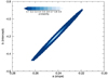 |
Fig. 1. Normalized 2D posterior probability of the distance-scale parameters obtained from the sample of PN calibrators with σϖc/ϖc< 20%. |
By adopting different thresholds on the relative DR3 parallax error σϖc/ϖc, we inferred different scale parameters, giving consistent estimates of the scale slope a and intercept b, as reported in Table 2. Figure 2 shows the log R − log SHβ plane with the subsets of calibrators for which σϖ/ϖ ≤ 10% (top panel) and σϖc/ϖc ≤ 20% (bottom panel) along with their error bars, and the corresponding estimated linear relation (see caption).
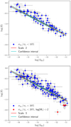 |
Fig. 2. Log(R) [pc] vs. log(SHβ) [erg cm−2 s−1] plot for calibrators with σϖc/ϖc < 0.1 (top panel) and σϖc/ϖc < 0.2 (bottom panel). In both plots, the blue points are the calibrators. Their logarithmic (asymmetric) error bars reflect the 1σ uncertainties of the observed parameters. In the bottom plot, the red points are the calibrators with log Mi < −2. The red line shows the two distance scales from the calibrators, and in cyan, we plot the 2σ confidence band of the scales, representing the uncertainty of the logarithmic radius R induced by the correlated errors on |


Summary of the distance-scale analysis.
An inspection of these plots shows that both data sets present a somewhat large dispersion around the scale. Moreover, from a comparison of the 20% sample of Fig. 2 with that of Fig. 2 in Paper I (where the calibration used DR2 parallaxes), we note that the numerous stragglers populating the lower right end of the plane, which correspond to PN with very low ionized mass (log Mi < −2), are not so prominent in the new plots.
In the complete set of potential calibrators, 37 objects had log Mi < −2, but the parallaxes of none of them were accurate enough at the 10% level, and only a few (indicated in red in the lower panel of Fig. 2) met the 20% requirement. When we placed these 37 objects on the log RPN − log SHβ plane, they were scattered mainly in the lower part of the graph, and their distance did not conform with the statistical scale. This corroborates the findings of our previous paper based on DR2 data.
To further investigate the ionized-mass effect, we inspected the PNe with σϖc/ϖc < 20% by displaying their log Mi on a color-density scale. The result, shown in Fig. 3, is quite striking and can be fully appreciated through the quality of the calibrators: The dispersion around the linear scale is clearly linked to the (estimated) log Mi of the PN shell, manifesting the deviation of its actual evolutionary state. In the transition from ionization-bound, or optically thick, to density-bound, or optically thin, the ionized mass of PN increases, as discussed in Pottasch (1980). Therefore, the model assumption of fully ionized, constant mass, on which Eq. (1) stands, does not strictly hold.
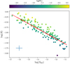 |
Fig. 3. Log(R) [pc] vs. log(SHβ) [erg cm−2 s−1] plot for the PN sample with σϖc/ϖc < 0.2, color-coded according to their ionized mass. The error bars have been omitted for clarity. The cross in the bottom left corner is representative of the typical error on the respective axis. |
Remarkably, when we tried to tighten the constraint on the goodness of the parallax relative error even more, we obtained a similar dispersion of the calibrators as in Fig. 3. Finally, by subtracting the effect due to the nominal uncertainties of the observed angular radius and flux, we tentatively estimated an average intrinsic (cosmic) scatter of ∼0.1 dex around the distance scale, and we conclude that this is due to an actual observed nebular evolution that limits the potential accuracy of this statistical distance scale, unless the ionized mass of the PN is known a priori.
The results of the calibration are reported in Table 2, where for each of the three relative uncertainty thresholds on σϖc/ϖc, we give the number of calibrators Ncal and the estimated slope and intercept along with their correlation ρab. We also list the averaged parameter  , which ideally, is equal to 1, and its dispersion ⟨σK⟩, which is an indicator of the goodness of the scale (see Smith 2015).
We used the third scale listed in Table 2, which is calibrated with central stars whose DR3 parallaxes were measured with an uncertainty better than 20%, which has a ⟨K⟩∼0.964. Through the analysis presented in this paper, we have confirmed that using another of the three scales would not affect the science results. Our adopted scale is
 (4)
(4)
In Table 3 we list the new catalog of distances of 843 Galactic PNe, based on Eq. (4). For each PN in the HASH catalog whose Hβ intensity and apparent radius is available, we calculated its heliocentric distance, D, based on our scale.
Catalog of statistical distances and peculiar velocities of Galactic PNe.
In the catalog, we list the PN G name, the angular radius θ, the logarithmic Hβ flux and its uncertainty, the logarithmic extinction constant and its uncertainty, the heliocentric distances from our scale of Eq. (4), D [kpc], and their left and right formal uncertainties. The latter were computed by estimating σlogD via first-order error propagation of the linear relations among the variables log R, log SHβθ, and D, accounting for uncertainties in both observed and fitted parameters; then, asymmetric uncertainties were defined as σD− = 10(log D − σlogD) and σD+ = 10(log D + σlogD). Finally, we included the PN peculiar velocity Vpec and its uncertainty calculated from Eq. (12), plus a disk, bulge, and halo population classification, as discussed in the following section.
3. Planetary nebulae as tracers of the Galactic disk
An important scientific motivation for the Galactic PN distance scale is the study of the radial (and vertical) metallicity gradients in the Galaxy.
Planetary nebulae are the ejecta of evolved 1–8 M⊙ stars, thus they represent a continuum of stellar populations from very old through relatively young, with ages ∼0 to ∼10 Gyr, which makes them very versatile probes for Galactic evolution. Gas-phase abundances of α-elements observed through emission lines and measured in their shell should be the same as those of their progenitors at the time of formation because these elements do not change much during the evolution of these stars. Thus, tracing the abundances of these elements is equivalent to probing the Galaxy abundance with a look-back time from ∼0 to ∼10 Gyr, depending on the initial progenitor mass of the PNe.
3.1. Elemental abundances
We used PN elemental abundances both for progenitor-dating purposes and to determine the metallicity gradients. We selected the elemental abundances from all references included in Stanghellini & Haywood (2018), to which we added the abundances from the data sets by Tsamis et al. (2003), Miller et al. (2019), McNabb et al. (2016), and Delgado-Inglada et al. (2015), which were not included therein. In the references where the abundances are given both for the whole nebula and for different parts of the PN, we used only the measures that were based on spectra of the whole PN, so that the abundances from different references are readily comparable with one another. The final abundances were curated, that is, we recalculated the ionization correction factor (ICF) uniformly, as described in Stanghellini & Haywood (2018).
In Table 4 we list the average abundances used in this paper. Column (1) gives the PN G name, and in Cols. (2) through (4) we give the C, N, and O abundances in the usual scale log(X/H) + 12, averaged from all the available references. The uncertainties, given in dex, are the dispersion of that elemental abundance across the literature, estimated with σ(log(O/H)) = 0.434 × [σ(O/H)/⟨O/H⟩]. We also produced a curated catalog of selected PN abundances, shown in Table 5. For this selection, we prioritized abundances from space-based observations unless they were deemed uncertain in the original papers; otherwise, we used the published ground-based abundances, prioritizing the most recent, or recently revised, abundances. Curated abundances are given with their uncertainty when available in the original reference.
Averaged elemental abundances of Galactic PNe.
Selected elemental abundances of Galactic PNe.
3.2. Velocities of the central stars of PNe
For a sizable sample of CSPNe with a statistical distance from our catalog, Gaia DR3 provides equatorial proper motions μα* ± σμα*3, μδ ± σμδ. We used this kinematic information as insight for their populations and ages. After converting DR3 proper motions and their standard deviations into galactic coordinates μl ± σμl, μb ± σμb via the transformation matrices  and CGal defined by Eqs. (4.62) and (4.79) of the Gaia EDR3 online documentation4, we computed the corresponding observed spatial velocities plus errors, given in [km s−1], as
 (5)
(5)
 (6)
(6)
where l and b are the Galactic longitude and latitude. We also adopted σD ≡ (σD− + σD+)/2. The third component of the velocity is the radial component, Vr, which has been observed independently for 498 PNe of our sample (Durand et al. 1998)5.
Having secured distances and kinematic data for these stars, we can estimate their peculiar velocity Vpec as the residual stellar motion that does not conform to the general Galactic rotation. To this end, we assumed an empirical model for the Galactic rotation curve that follows Eilers et al. (2019) for galactocentric distances larger than 5 kpc, while for inner distances, we made use of the results of Bhattacharjee et al. (2014), who resorted to H I and H II regions, as well as CO emission lines, as tracers of the inner Galactic disk. We adapted the results of Bhattacharjee et al. (2014) to the fundamental parameters found by Eilers et al. (2019), that is, R⊙ = 8.122 kpc, the galactocentric distance of the Sun, and VLSR = 229 [km s−1], the circular velocity of the local standard of rest (LSR). We combined these data into a grid of Galactic radii and corresponding rotation velocities, plus uncertainties, as given in Table 6. Moreover, in the following calculations, the velocity of the Sun with respect to the LSR was set to (U⊙, V⊙, W⊙) = (11.1, 12.4, 7.25) [km s−1], according to Schönrich et al. (2010).
Adopted Galactic rotation curve.
We first transformed the observed spatial velocities into Cartesian components along the local triad at the star as
 (7)
(7)
where  ,
,  ,
,  , and A is the so-called direction cosine matrix representing the rotation to the local frame.
To derive galactocentric velocities, we must account for the galactocentric velocity of the Sun, that is, v⊙ = (U⊙, V⊙ + VLSR, W⊙), so that
 (8)
(8)
For the following analysis, it is useful to express spatial velocities in cylindrical coordinates, for which we need to compute the galactocentric azimuth ϕ as (e.g., López-Corredoira & Sylos Labini 2019)
 (9)
(9)
where D is the heliocentric distance of the star, and ϕ is taken as positive in the direction of galactic rotation; the radial, azimuthal, and vertical components of the spatial velocity are then given by
 (10)
(10)
Finally, we are able to estimate the peculiar velocity of each star by subtracting the circular motion due to differential galactic rotation from the azimuthal component Vϕ. To do this, we computed for each PN the galactocentric radius RG projected onto the Galactic plane as
 (11)
(11)
and we interpolated linearly between the nearest two values of RG of Table 6 to calculate the circular stellar velocity Vc(RG).
The absolute space motion of the stars (or the PNe), which we call Vpec, can be obtained by quadrature of the three velocity components as
 (12)
(12)
where σVpec is a lower-limit uncertainty, which assumes uncorrelated variables and a perfect model. The peculiar velocities for the PNe are reported in Table 3.
In Fig. 4 we placed the inferred peculiar velocities in the so-called Toomre diagram, which can be used to identify regions in which the probability of finding disk versus halo stars is high. In particular, following Bonaca et al. (2017), we used Vpec > 220 [km s−1] as the threshold value for rejecting halo stars.
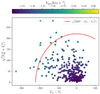 |
Fig. 4. Halo PNe selected through the velocity analysis of the CSPNe by means of the Toomre diagram. The color bar is coded for the peculiar velocities as in Eq. (12). The dots outside the region encircled by the red curve correspond to halo PNe. |
3.3. Galactic PN populations, and dating PN progenitors
We derived heliocentric distances D and their confidence limits, as described in Sect. 2.3, for 843 Galactic PNe. The range of distances spanned by these PNe is ∼150 to ∼27 000 [pc], and most of them can be included in a general disk population, thus they are adequate for our science scope. We populate the halo PN sample selecting them by peculiar velocity, where halo PNe have Vpec > 220 [km s−1]. This selection yields 13 halo PNe. We also tentatively defined the bulge population similarly to Stanghellini & Haywood (2018) by selecting the PNe in the central 3 × 3 [kpc], that is, with |z|< 3 and 0 < RG < 3 [kpc]. To constrain the bulge sample even more, we selected in this sample only the PNe whose apparent radius was θ < 5″. Our selection gives 102 bulge PNe. Whether a PN belongs to the halo or bulge populations according to our selection is noted in Table 3.
In Fig. 5 we plot the distribution of the peculiar velocity versus vertical height z, where the color indicates the distance from the Galactic center. In the area between the two gray lines (±0.175 kpc) PNe with high peculiar velocity are away from the Galactic center. It is worth noting that all bulge PNe selected as in Sect. 3.3 are outside the gray lines and have an intermediate Vpec.
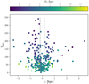 |
Fig. 5. Galactic distribution of Vpec from Eq. (12), with Galactic altitude, where the color is coded for the distance from the Galactic center RG. The vertical thin lines encompass the |z|< 0.175 zone. |
Dating PN progenitors is not trivial, and it has been attempted by Peimbert and Torres-Peimbert by dividing Galactic PNe into populations (i.e., PN types I through V). This approach uses both the chemistry of the PNe and their kinematics. Stanghellini & Haywood (2018) used the final yields of the evolutionary elements compared to nebular abundances of carbon and nitrogen to select two PN progenitor populations with extreme ages, called OPPNe (old progenitors PNe, with progenitor ages > 7.5 Gyr), and YPPNe (young progenitors PNe, with progenitor ages < 1 Gyr). This selection is based on the observation that PNe with old and young progenitors occupy markedly different loci on the N/H versus C/H, and N/H versus O/H, planes. Fig. 2 of Ventura et al. (2016) was used to determine that OPPNe have C/H > N/H or [log(N/H) + 12] < 0.8 × [log(O/H) + 12] + 1.4 and YPPNe have C/H < N/H or [log(N/H) + 12] > 0.6 × [log(O/H) + 12] + 3.3. In Tables 4 and 5, Col. 5, we list the PN progenitor age group as derived above, when available.
More insight into dating PN progenitors is derived from the comparison of Gaia proper motions described in the previous subsection, with the ages derived purely from the PN chemistry above. In Fig. 6 we show the resulting distribution of Vpec for the general PN population (which includes OPPNe, YPPNe, and the intermediate-age progenitor PNe, and the PNe whose age from chemistry was unavailable), then by plotting separately OPPNe and YPPNe. We find that the OPPNe distribution peaks at Vpec ∼ 60 [km s−1], while the YPPNe distribution peaks at a lower velocity (∼25 − 30 [km s−1]). This plot shows the correlation between completely independent dating systems from the chemistry and the kinematics of the PNe, giving us confidence about using the OPPNe and YPPNe distributions.
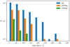 |
Fig. 6. Histogram of the spatial peculiar velocity Vpec [km s−1] for the general disk population and for the OPPNe and YPPNe separately. The velocity bin is 10 km s−1. The y-axis is in logarithmic scale. |
3.4. Galactic metallicity gradients and other metallicity variations
The radial metallicity gradients in this paper were calculated by orthogonal distance regression, which makes use of the uncertainties in the measured quantities RG and log(O/H) + 12. The uncertainties in the elemental abundances are described in Sect. 3.1, where we indicate the literature fonts from which we chose the abundances and how the errors were estimated both in the average and chosen abundances (see Table 4). The uncertainties in RG were computed by first-order propagation of the symmetrized error of the distance scale, σD = (σD− + σD+)/2, thus obtaining σRG = |Dcos2b − R⊙ cos l cos b|⋅σD/RG. The regression yields a slope and an intercept, along with their formal errors.
In Table 7 we present the estimates of the gradient slopes obtained using different subsets of PNe, and with both averaged and selected chemical abundances. We used all PNe for which at least one oxygen measurement was available in the literature, excluding only the extreme outliers (log(O/H) + 12 < 7.5 and log(O/H) + 12 > 9). All radial oxygen gradients that we derive in this paper have negative slopes. The general PN population (Fig. 7) has a gradient slope of −0.0144 ± 0.00385 [dex kpc−1] when we use the average abundances. When the halo population (3 PNe) is excluded, the gradient does not change significantly.
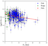 |
Fig. 7. Radial oxygen gradients for the complete PN sample for which we have a statistical distance and at least one O/H measurement in the literature. Oxygen abundances are averages of all published abundances, and the error bars represent the dispersion. All PNe have been included in these plots, and halo and bulge populations are indicated with different colors. The red line is the linear fit to the data. The slopes and intercepts for the different populations are listed in Table 7. |
Radial oxygen gradients.
For all comparable samples, the gradients steepen with time since Galaxy formation. For the OPPN and YPPN populations, we derived gradient slopes Δlog(O/H)/ΔRG = −0.0121 ± 0.00465 and −0.022 ± 0.00758 [dex kpc−1], respectively, when we used average abundances, and Δlog(O/H)/ΔRG = −0.0132 ± 0.00464 and −0.0278 ± 0.00789 [dex kpc−1], respectively, when we used the selected abundances (plots in Fig. 8). This result indicates a mild evolution, that is significant when compared to the uncertainties, of the metallicity gradient with time. Our results point to a steeper gradient slope for the younger stellar population than for the older stellar population, with a slope difference of ∼0.15 dex. This implies a slow time evolution of the gradient. The time evolution of the gradient slope does not vary, regardless of whether we include halo PNe in the OPPN sample (see Table 7).
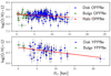 |
Fig. 8. Radial oxygen gradients for the OPPN (top) and the YPPN (bottom) populations. All PNe have been included in these plots, and halo and bulge populations are indicated with different colors. Oxygen abundances are those selected here. The red lines are the linear fits of the data. The slopes and intercepts for the different populations are listed in Table 7. |
It is beyond the scope of this paper to discuss the causes for the steepening gradient. Chemical evolutionary models of star-forming galaxies (Gibson et al. 2013) indicate that the radial metallicity gradients steepen with time when the chemical evolution proceeds with feedback of fresh, metal-poor gas from the environment. Models like this cannot predict the gradient ab initio. The metallicity gradients for old populations such as those from OPPNe therefore represent a valuable constraint.
Finally, we tested the oxygen evolution (or chemical enrichment) by comparing average oxygen abundances in the OPPNe and YPPNe samples to derive an average Galactic enrichment of ∼0.06 dex between the age > 7.5 Gyr and the age < 1 Gyr populations.
4. Results and conclusions
This paper yields essentially three novel results for PNe in the Galactic environment. First, we produced a new distance scale based on DR3 parallaxes, which is given in Eq. (4). The distances derived from the new scale are published as a catalog in this paper (Table 3). By comparing our new distances with the CSPN DR3 parallaxes, as in the analysis by Smith (2015), we find ⟨K⟩ = 0.964, where K = D × ϖc, and ⟨σK⟩ = 0.154 when we exclude the PNe with log Mi < −2 from the comparison, and ⟨K⟩ = 0.931 when we include all calibrators. Comparing these results with those of Paper I, where the best scale obtained with DR2 parallaxes gave ⟨K⟩ = 0.948 and ⟨σK⟩ = 0.25, we conclude that the use of DR3 parallaxes as calibrators successfully improved upon the Galactic PN distance scale.
We have calculated ⟨K⟩ based on DR3 parallaxes for the most commonly used PN distance scales, such as Frew et al. (2016, hereafter FPB) and Stanghellini et al. (2008, hereafter SSV). We found ⟨KFPB⟩=⟨DFPB × ϖc⟩ = 1.272 and ⟨KSSV⟩=⟨DSSV × ϖc⟩ = 1.203 with the exclusion of calibrators with log Mi < −2, and ⟨KFPB⟩ = 1.36 and < KSSV⟩ = 1.29 when all calibrators are included. We conclude that the scale presented in Eq. (4) gives the most reliable distances to date, and the distances in Table 3 should be used, unless an accurate parallax measurement of the central star of PN under study is available, from DR3 or otherwise. Moreover, our analysis revealed that the log RPN − log SHβ distance scale of Galactic PNe has an intrinsic mean dispersion of ≈0.1 dex around the log RPN − log SHβ linear relation, which can be accounted for by the variation in the PN ionized mass (excluding objects with log Mi < −2), bringing us to the conclusion that statistical distance scales such as this can hardly be improved by increasing the accuracy of calibrators.
Second, we used the Gaia DR3 proper motion for thorough description of the peculiar velocities of the CSPNe, and to characterize the halo population. The peculiar velocity derivation has the additional advantage to be a completely independent assessment of the progenitor ages of the PNe, thus validating even further the OPPN and YPPN classes based on elemental abundance ratios C/O and N/O. The proper motion and peculiar velocity analysis of Sect. 3.2 provided a tool for excluding halo PNe from the gradient analysis. Even more importantly, it gave us additional confidence in the progenitor dating from chemical analysis, as described in Sect. 3.3. To our knowledge, this is the first time that dating PNe is consistent with two completely independent approaches, while in the past, the dating scheme has used either approach, or both approaches for different age classes, such as in defining Peimbert’s PN types (Peimbert 1978). Dating PN progenitors is essential to study the time evolution of the radial metallicity gradients in the Milky Way.
Third, we measured the radial oxygen gradients based on DR3 distance scale, with halo PNe selected through their kinematic properties measured by Gaia DR3, and progenitor ages from chemical evolutionary assessment, confirmed via the peculiar velocities determined by Gaia. The negative shallow gradients that we determined and the mild evolution of the gradients, which steepened since the formation of the Galaxy, are a confirmation of past results both in the Galaxy (Stanghellini & Haywood 2018) and in the nearby spiral galaxies examined (Peña & Flores-Durán 2019; Magrini et al. 2016), where all emission-line probes in star-forming galaxies (including the Milky Way) indicate that the oxygen radial gradients are steeper in the younger populations. For the gradients, we used curated catalogs of published abundances, which we give in Tables 4 and 5.
It is worth noting that while our results confirm most of the metallicity gradients measurements based on gas-phase data published to date, recent cluster and stellar results show a more controversial picture (Anders et al. 2017; Magrini et al. 2023; Gaia Collaboration 2023a). Stellar metallicity are mainly inferred from iron rather than oxygen. Because iron atoms in PNe are mostly found in condensed state (e.g., Delgado-Inglada et al. 2015), a direct comparison between the stellar and nebular samples is typically problematic.
The work of Magrini et al. (2023) also included α-element gradients, indicating very little oxygen gradient evolution, compatible with flattening of gradients with time. Their oxygen gradient slopes of the age < 1 Gyr and age > 3 Gyr bins in their Table A.10. are the same within the uncertainties. We underline that these results are compatible with ours if we take into account the different age ranges used: our PN progenitors are in the age < 1 Gyr and age > 7.5 Gyr bins, whereas their oldest clusters are within 7 Gyr. Furthermore, migration and evolution due to inflow of clusters and stars may be different in ways that are unpredictable when measuring radial gradients.
Interestingly, Bhattacharya et al. (2022), who studied the radial oxygen gradients in M 31, found that young thin-disk PNe describe a steeper radial gradient than the older thick-disk population. This agrees qualitatively with our results, where radial metallicity gradients steepen with galaxy evolution. Quantitatively, they attempted to unify the gradients slopes across galaxies in their Fig. 13 by taking disk scale lengths into account, and they showed remarkable similarities between oxygen gradients in the Galaxy and M 31.
More inspection of Galactic gradients from data and modeling comes from the recent analysis in Lian et al. (2023), who used integrated radial metallicities to find (see their Fig. 1) that radial Fe/H gradients from older populations are flatter than for the young population. This agrees with our results. They also compared the Galactic gradient from present-day stellar population with that obtained from gas-phase oxygen (H II region), which is consistent with the PNe abundance tracers. This reinforces the confidence in our findings.
The distance scale that we presented here and the distances in our catalog will be used in the future to study the behavior of dust and other elements in Galactic PNe in the framework of the chemical evolution of the Galaxy.
The list includes all objects from the HASH database that were labeled as ‘TRUE PN’ at the time of this work.
When Gaia BP/RP broadband photometry is not available, the source color is an additional parameter estimated from the Gaia astrometric solution through the chromaticity effect.
The asterisk, indicating that the longitudinal proper motion is measured along the great circle at the star’s location, will be dropped and implicitly assumed in the following.
https://gea.esac.esa.int/archive/documentation/GEDR3/Data_processing/chap_cu3ast/sec_cu3ast_intro/ssec_cu3ast_intro_tansforms.html#SSS1
Gaia DR3 had measured radial velocities for only 13 CSPNe of our calibrator sample.
Acknowledgments
This work has made use of data from the European Space Agency (ESA) mission Gaia (https://www.cosmos.esa.int/gaia), processed by the Gaia Data Processing and Analysis Consortium (DPAC, https://www.cosmos.esa.int/web/gaia/dpac/consortium). Funding for the DPAC has been provided by national institutions, in particular the institutions participating in the Gaia Multilateral Agreement. B.B. acknowledges the support of the Italian Space Agency (ASI) through contract 2018-24-HH.0 and its addendum 2018-24-HH.1-2022 to the National Institute for Astrophysics (INAF). The authors would like to thank the anonymous referee whose comments and suggestions helped improving the original manuscript.
References
- Anders, F., Chiappini, C., Minchev, I., et al. 2017, A&A, 600, A70 [NASA ADS] [CrossRef] [EDP Sciences] [Google Scholar]
- Bhattacharjee, P., Chaudhury, S., & Kundu, S. 2014, ApJ, 785, 63 [NASA ADS] [CrossRef] [Google Scholar]
- Bhattacharya, S., Arnaboldi, M., Caldwell, N., et al. 2022, MNRAS, 517, 2343 [NASA ADS] [CrossRef] [Google Scholar]
- Bonaca, A., Conroy, C., Wetzel, A., et al. 2017, ApJ, 845, 101 [NASA ADS] [CrossRef] [Google Scholar]
- Buckley, D., & Schneider, S. E. 1995, ApJ, 446, 279 [NASA ADS] [CrossRef] [Google Scholar]
- Chornay, N., & Walton, N. A. 2021, A&A, 656, A51 [NASA ADS] [CrossRef] [EDP Sciences] [Google Scholar]
- Curti, M., Maiolino, R., Cirasuolo, M., et al. 2020, MNRAS, 492, 821 [CrossRef] [Google Scholar]
- Delgado-Inglada, G., Rodríguez, M., Peimbert, M., et al. 2015, MNRAS, 449, 1797 [NASA ADS] [CrossRef] [Google Scholar]
- Durand, S., Acker, A., & Zijlstra, A. 1998, A&AS, 132, 13 [NASA ADS] [CrossRef] [EDP Sciences] [Google Scholar]
- Eilers, A.-C., Hogg, D. W., Rix, H.-W., et al. 2019, ApJ, 871, 120 [Google Scholar]
- Fabricius, C., Luri, X., Arenou, F., et al. 2021, A&A, 649, A5 [NASA ADS] [CrossRef] [EDP Sciences] [Google Scholar]
- Frew, D. J., Parker, Q. A., & Bojičić, I. S. 2016, MNRAS, 455, 1459 [Google Scholar]
- Gaia Collaboration (Prusti, T., et al.) 2016, A&A, 595, A1 [NASA ADS] [CrossRef] [EDP Sciences] [Google Scholar]
- Gaia Collaboration (Recio-Blanco, A., et al.) 2023a, A&A, 674, A38 [CrossRef] [EDP Sciences] [Google Scholar]
- Gaia Collaboration (Vallenari, A., et al.) 2023b, A&A, 674, A1 [NASA ADS] [CrossRef] [EDP Sciences] [Google Scholar]
- Gibson, B. K., Pilkington, K., Brook, C. B., et al. 2013, A&A, 554, A47 [CrossRef] [EDP Sciences] [Google Scholar]
- González-Santamaría, I., Manteiga, M., Manchado, A., et al. 2021, A&A, 656, A51 [NASA ADS] [CrossRef] [EDP Sciences] [Google Scholar]
- Henry, R. B. C., Kwitter, K. B., Jaskot, A. E., et al. 2010, ApJ, 724, 748 [NASA ADS] [CrossRef] [Google Scholar]
- Lian, J., Bergemann, M., Pillepich, A., Zasowski, G., & Lane, R. R. 2023, Nat. Astron., 7, 951 [CrossRef] [Google Scholar]
- Lindegren, L., Bastian, U., Biermann, M., et al. 2021a, A&A, 649, A4 [EDP Sciences] [Google Scholar]
- Lindegren, L., Klioner, S. A., Hernández, J., et al. 2021b, A&A, 649, A2 [EDP Sciences] [Google Scholar]
- López-Corredoira, M., & Sylos Labini, F. 2019, A&A, 621, A48 [NASA ADS] [CrossRef] [EDP Sciences] [Google Scholar]
- Mackereth, J. T., Bovy, J., Leung, H. W., et al. 2019, MNRAS, 489, 176 [Google Scholar]
- Magrini, L., Coccato, L., Stanghellini, L., et al. 2016, A&A, 588, A91 [NASA ADS] [CrossRef] [EDP Sciences] [Google Scholar]
- Magrini, L., Viscasillas Vázquez, C., Spina, L., et al. 2023, A&A, 669, A119 [NASA ADS] [CrossRef] [EDP Sciences] [Google Scholar]
- Matteucci, F. 2021, A&ARv, 29, 5 [NASA ADS] [CrossRef] [Google Scholar]
- McNabb, I. A., Fang, X., & Liu, X.-W. 2016, MNRAS, 461, 2818 [NASA ADS] [CrossRef] [Google Scholar]
- Miller, T. R., Henry, R. B. C., Balick, B., et al. 2019, MNRAS, 482, 278 [NASA ADS] [Google Scholar]
- Parker, Q. A., Bojičić, I. S., & Frew, D. J. 2016, J. Phys. Conf. Ser., 728, 032008P [NASA ADS] [CrossRef] [Google Scholar]
- Peña, M., & Flores-Durán, S. N. 2019, Rev. Mex. Astron. Astrofis., 55, 255 [Google Scholar]
- Peimbert, M. 1978, in Planetary Nebulae, ed. Y. Terzian (Dordrecht: Reidel), IAU Symp., 76, 215 [NASA ADS] [Google Scholar]
- Pottasch, S. R. 1980, A&A, 89, 336 [NASA ADS] [Google Scholar]
- Prantzos, N., Abia, C., Chen, T., et al. 2023, MNRAS, 523, 2126 [NASA ADS] [CrossRef] [Google Scholar]
- Schneider, S. E., & Buckley, D. 1996, ApJ, 459, 606 [NASA ADS] [CrossRef] [Google Scholar]
- Schönrich, R., Binney, J., & Dehnen, W. 2010, MNRAS, 403, 1829 [NASA ADS] [CrossRef] [Google Scholar]
- Shklovsky, I. S. 1956, AZh, 33, 222 [NASA ADS] [Google Scholar]
- Smith, H. 2015, MNRAS, 449, 2980 [CrossRef] [Google Scholar]
- Stanghellini, L. 2019, IAU Symp., 343, 174 [NASA ADS] [Google Scholar]
- Stanghellini, L., & Haywood, M. 2018, ApJ, 862, 45 [Google Scholar]
- Stanghellini, L., Shaw, R. A., & Villaver, E. 2008, ApJ, 689, 194 [NASA ADS] [CrossRef] [Google Scholar]
- Stanghellini, L., Berg, D., Bresolin, F., Cunha, K., & Magrini, L. 2019, arXiv e-prints [arXiv:1905.04096] [Google Scholar]
- Stanghellini, L., Bucciarelli, B., Lattanzi, M. G., & Morbidelli, R. 2020, ApJ, 889, 21 [Google Scholar]
- Strömberg, G. 1925, ApJ, 61, 363 [NASA ADS] [CrossRef] [Google Scholar]
- Strömberg, G. 1946, ApJ, 104, 12 [Google Scholar]
- Tsamis, Y. G., Barlow, M. J., Liu, X. W., Danziger, I. J., & Storey, P. J. 2003, MNRAS, 345, 186 [NASA ADS] [CrossRef] [Google Scholar]
- Ventura, P., Stanghellini, L., Di Criscienzo, M., García-Hernández, D. A., & Dell’Agli, F. 2016, MNRAS, 460, 3940 [NASA ADS] [CrossRef] [Google Scholar]
- Wielen, R. 1977, A&A, 60, 263 [NASA ADS] [Google Scholar]
All Tables
All Figures
|
Fig. 1. Normalized 2D posterior probability of the distance-scale parameters obtained from the sample of PN calibrators with σϖc/ϖc< 20%. |
| In the text | |
|
Fig. 2. Log(R) [pc] vs. log(SHβ) [erg cm−2 s−1] plot for calibrators with σϖc/ϖc < 0.1 (top panel) and σϖc/ϖc < 0.2 (bottom panel). In both plots, the blue points are the calibrators. Their logarithmic (asymmetric) error bars reflect the 1σ uncertainties of the observed parameters. In the bottom plot, the red points are the calibrators with log Mi < −2. The red line shows the two distance scales from the calibrators, and in cyan, we plot the 2σ confidence band of the scales, representing the uncertainty of the logarithmic radius R induced by the correlated errors on |
| In the text | |
|
Fig. 3. Log(R) [pc] vs. log(SHβ) [erg cm−2 s−1] plot for the PN sample with σϖc/ϖc < 0.2, color-coded according to their ionized mass. The error bars have been omitted for clarity. The cross in the bottom left corner is representative of the typical error on the respective axis. |
| In the text | |
|
Fig. 4. Halo PNe selected through the velocity analysis of the CSPNe by means of the Toomre diagram. The color bar is coded for the peculiar velocities as in Eq. (12). The dots outside the region encircled by the red curve correspond to halo PNe. |
| In the text | |
|
Fig. 5. Galactic distribution of Vpec from Eq. (12), with Galactic altitude, where the color is coded for the distance from the Galactic center RG. The vertical thin lines encompass the |z|< 0.175 zone. |
| In the text | |
|
Fig. 6. Histogram of the spatial peculiar velocity Vpec [km s−1] for the general disk population and for the OPPNe and YPPNe separately. The velocity bin is 10 km s−1. The y-axis is in logarithmic scale. |
| In the text | |
|
Fig. 7. Radial oxygen gradients for the complete PN sample for which we have a statistical distance and at least one O/H measurement in the literature. Oxygen abundances are averages of all published abundances, and the error bars represent the dispersion. All PNe have been included in these plots, and halo and bulge populations are indicated with different colors. The red line is the linear fit to the data. The slopes and intercepts for the different populations are listed in Table 7. |
| In the text | |
|
Fig. 8. Radial oxygen gradients for the OPPN (top) and the YPPN (bottom) populations. All PNe have been included in these plots, and halo and bulge populations are indicated with different colors. Oxygen abundances are those selected here. The red lines are the linear fits of the data. The slopes and intercepts for the different populations are listed in Table 7. |
| In the text | |
Current usage metrics show cumulative count of Article Views (full-text article views including HTML views, PDF and ePub downloads, according to the available data) and Abstracts Views on Vision4Press platform.
Data correspond to usage on the plateform after 2015. The current usage metrics is available 48-96 hours after online publication and is updated daily on week days.
Initial download of the metrics may take a while.