| Issue |
A&A
Volume 638, June 2020
|
|
|---|---|---|
| Article Number | A127 | |
| Number of page(s) | 18 | |
| Section | Astrophysical processes | |
| DOI | https://doi.org/10.1051/0004-6361/201936143 | |
| Published online | 25 June 2020 | |
Colors and patterns of black hole X-ray binary GX 339-4
1
Department of Physics and Astronomy, University of Turku, 20014 Turku, Finland
e-mail: This email address is being protected from spambots. You need JavaScript enabled to view it.
2
Department of Astrophysics, St. Petersburg State University, Universitetskiy pr. 28, Peterhof, 198504 St. Petersburg, Russia
3
Nordita, KTH Royal Institute of Technology and Stockholm University, Roslagstullsbacken 23, 10691 Stockholm, Sweden
4
Space Research Institute of the Russian Academy of Sciences, Profsoyuznaya Str. 84/32, 117997 Moscow, Russia
5
Institut für Astronomie und Astrophysik, Kepler Center for Astro and Particle Physics, Universität Tübingen, Sand 1, 72076 Tübingen, Germany
6
Kazan (Volga region) Federal University, Kremlevskaya str. 18, Kazan 420008, Russia
Received:
20
June
2019
Accepted:
23
April
2020
Abstract
Black hole X-ray binaries show signs of nonthermal emission in the optical to near-infrared range. We analyzed optical to near-infrared SMARTS data on GX 339-4 over the 2002–2011 period. Using soft state data, we estimated the interstellar extinction toward the source and characteristic color temperatures of the accretion disk. We show that various spectral states of regular outbursts occupy similar regions on color-magnitude diagrams, and that transitions between the states proceed along the same tracks despite substantial differences in the morphology of the observed light curves. We determine the typical duration of hard-to-soft and soft-to-hard state transitions and the hard state at the decaying stage of the outburst to be one, two, and four weeks, respectively. We find that the failed outbursts cannot be easily distinguished from the regular outbursts at their early stages, but if the source reaches 16 mag in V band, it transits to the soft state. By subtracting the contribution of the accretion disk, we obtain spectra of the nonthermal component, which have constant, nearly flat shapes during the transitions between the hard and soft states. In contrast to the slowly evolving nonthermal component seen at optical and near-infrared wavelengths, the mid-infrared spectrum is strongly variable on short timescales and sometimes shows a prominent excess with a cutoff below 1014 Hz. We show that the radio to optical spectrum can be modeled using three components corresponding to the jet, hot flow, and irradiated accretion disk.
Key words: accretion, accretion disks / black hole physics / methods: data analysis / stars: black holes / stars: individual: GX 339-4 / X-rays: binaries
© ESO 2020
1. Introduction
GX 339-4 is a well-studied black hole (BH) low-mass X-ray binary (LMXB) that was discovered as a bright and variable X-ray source using the Orbiting Solar Observatory 7 (Markert et al. 1973). The source is known to undergo recurrent outbursts every two to three years and it has become a standard target for multiwavelength campaigns (Homan et al. 2005; Belloni et al. 2005, 2006; Tomsick et al. 2008; Shidatsu et al. 2011; Cadolle Bel et al. 2011; Motta et al. 2011; Rahoui et al. 2012; Buxton et al. 2012; Corbel et al. 2013a). During outbursts the source undergoes a transition between different states that can be distinguished using a variety of criteria, including the X-ray hardness ratio, quasi-periodic oscillations, and other timing properties (Homan & Belloni 2005; McClintock et al. 2006; Remillard & McClintock 2006; Belloni et al. 2010).
The origin of these states is still not very well understood, but is generally associated with changes in the accretion flow geometry (see, e.g., Esin et al. 1997; Poutanen et al. 1997; Zdziarski et al. 2004; Done et al. 2007). In the soft X-ray state, the spectrum consists of a thermal component associated with a standard cold accretion disk (Shakura & Sunyaev 1973) and an additional power-law-like tail from the nonthermal corona (Poutanen & Coppi 1998; Gierliński et al. 1999; Zdziarski et al. 2001). In the hard state, the emission from the cold disk is greatly reduced owing to its truncation at a radius significantly larger than the radius of the innermost stable orbit; the emission instead is dominated by thermal Comptonization of some seed photons (cold disk and internal synchrotron) in an inner hot, geometrically thick accretion flow. The transitions between the spectral states happen because of a change in the truncation radius, which results in a variation of the relative contributions of the cold disk and hot flow, and also lead to corresponding changes in the timing properties (Done et al. 2007; Gilfanov, et al. 2010; Poutanen & Veledina 2014; De Marco et al. 2015; Stiele & Kong 2017; Poutanen et al. 2018; Mahmoud et al. 2019).
For many years it was known that the X-ray emitting region of accreting BHs is rather compact because of the fast variability observed in these objects. On the other hand, the optical to near-infrared (ONIR) emission was thought to originate mostly from an outer disk irradiated by the central X-ray source. We already had the first evidence that the situation is not so simple in the early 1980s, when the fast optical variability and quasi-periodic oscillations at 20 s were detected from GX 339-4 by Motch et al. (1982), which were interpreted as a signature of emission from the hot accretion flow or corona (Fabian et al. 1982). Soon after, Motch et al. (1983) carried out simultaneous optical and X-ray observations, which demonstrated a complicated structure of the cross-correlation function (CCF) with a precognition dip. Recently, similar CCFs were found in three BHs: XTE J1118+480 (Kanbach et al. 2001; Hynes et al. 2003a), Swift J1753.5-0127 (Durant et al. 2008, 2009, 2011; Hynes et al. 2009), and GX 339-4 (Gandhi et al. 2008, 2010). The shape of the CCF can be explained if the optical emission contains two components: synchrotron emission from the hot flow and reprocessed radiation, which are anti-correlated and correlated with the X-rays, respectively (Veledina et al. 2011). However, the shape of the CCF seems to be wavelength-dependent. For instance, the infrared versus X-ray CCF of GX 339-4 showed a single peak with no precognition dip (Casella et al. 2010), which was successfully explained by a jet model, in which the emission is powered by internal shocks (Malzac et al. 2018). Thus it is clear that the ONIR emission is not completely dominated by the accretion disk, but has at least one additional (nonthermal) component, either from the hot flow, or the jet, or both.
Signatures of this component are seen in the long-term variability as bright ONIR flares, which appear in the hard state (Hynes et al. 2000; Jain et al. 2001; Buxton & Bailyn 2004; Kalemci et al. 2013). Spectral evolution of the flare in XTE J1550-564 is consistent with the hot accretion flow scenario (Veledina et al. 2013; Poutanen & Veledina 2014). In Swift J1753.5-0127 the jet emission is known to be weak in radio and its contribution to the ONIR band is likely small (Durant et al. 2009), while the ONIR–X-ray broadband spectra can be explained well by the hot flow model (Kajava et al. 2016). On the other hand, the soft ONIR spectra of 4U 1543-47 (Kalemci et al. 2005) and MAXI J1836-194 (Russell et al. 2013) argue in favor of the jet scenario.
The origin of this nonthermal component can give us a clue to understanding the nature of the accretion-ejection engine operating in the vicinity of the BH. This aim can be reached by studying the evolution of its spectral shape throughout the outburst and in particular during the transitions between the states. This requires measurements of the interstellar extinction and subtraction of the (irradiated) accretion disk contribution. From this perspective, GX 339-4 is an interesting source because it has served as a target for numerous multiwavelength campaigns. The aim of this work is to study the behavior of the source spectrum on the color-magnitude diagram (CMD) and the evolution of the nonthermal component using spectral decomposition.
The paper is structured as follows. In Sect. 2, we describe the data used for the analysis. Section 3 contains details of the analysis, determination of the interstellar extinction, comparisons of different outbursts, and a determination of the spectrum of the nonthermal component. In Sect. 4 we discuss the observed ONIR properties and their connection to X-rays. We also discuss the origin of the nonthermal component in terms of the hot flow and jet models. We conclude in Sect. 5.
2. Data
Monitoring of GX 339-4 in the ONIR was conducted using the ANDICAM camera (DePoy et al. 2003) on the Small and Moderate Aperture Research Telescope System (SMARTS; Subasavage et al. 2010).1 We used the publicly available SMARTS data in V, I, J, and H filters taken in 2002–2011 (Buxton et al. 2012).2 We split the ONIR light curves into seven intervals, each covering one of the regular or failed outbursts (see Sect. 3.1). The light curves, corrected for the interstellar extinction (see Sect. 3.2), are shown in Fig. 1.
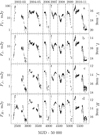 |
Fig. 1. Observed ONIR magnitudes and corrected for the interstellar extinction fluxes of GX 339-4 in four ONIR filters (V, I, J and H). Vertical dashed lines separate data into 7 intervals corresponding to each of the regular/failed outbursts. |
The X-ray data were taken from the Rossi X-ray Timing Explorer (RXTE) All-Sky Monitor (ASM)3 (Bradt et al. 1993), which provides observations of GX 339-4 in three energy ranges (1.5–3, 3–5, and 5–12 keV). The count rates from different channels were converted to the observed fluxes using an empirical linear relation from Zdziarski et al. (2002). We also made use of the Neil Gehrels Swift Observatory Burst Alert Telescope (Swift/BAT)4 (Gehrels et al. 2004; Barthelmy et al. 2005), which operates in the 15–150 keV range. The BAT, ASM A, and B light curves as well as the ASM B/A hardness ratio are shown in Fig. 2.
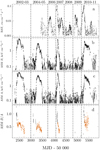 |
Fig. 2. X-ray light curves of GX 339-4. (a) Swift/BAT count rate in the 15–150 keV band, (b) ASM B (3–5 keV) flux, (c) ASM A (1.5–3 keV) light curve, and (d) ASM B/A hardness ratio. Orange points correspond to the soft states selected using ONIR data from four outbursts. Errors are 1σ. |
We adopted the mid-infrared (mid-IR) data, obtained by the Wide-field Infrared Survey Explorer satellite (WISE; Wright et al. 2010), from Gandhi et al. (2011). All reported 13 observations of GX 339-4 were taken during 24 hours on MJD 55265.88–55266.88, that is, within half a day from the SMARTS observation on MJD 55266.36 (Buxton et al. 2012). The mid-IR data were corrected for the interstellar extinction (see Sect. 2.2.3 in Gandhi et al. 2011).
We also used radio data obtained by the Australian Telescope Compact Array (ATCA; Wilson et al. 2011) in 5.5 and 9 GHz bands. Out of the two closest to the SMARTS and WISE quasi-simultaneous observations (MJD 55262.91 and 55269.80; see Table 1 in Corbel et al. 2013a) we selected the second, which has a positive slope at radio wavelengths and can be extrapolated to the mid-IR WISE data.
3. Light-curve analysis and results
3.1. Outburst phase separation
We used the ONIR light curves to split the regular outbursts, when GX 339-4 reaches the soft state, into different phases: the rising phase (RPh), the hard state at the rising stage (RHS), the transition from the hard to the soft state (HtS), the soft state (SS), the transition from the soft to the hard state (StH), the hard state at the decaying stage (DHS), the decaying phase (DPh), and quiescence (Q) (see Table 1). Different states were first roughly identified using X-ray data, as in Motta et al. (2009). We then fit an S- or Z-shaped curves to the ONIR data during the RPh, HtS, and StH phases and determined the transition dates. Further, we fit the broken power law to the DPh and Q data and obtained the start dates of quiescence. The details of the described procedure are explained in Appendix A and the start dates of each outburst phase (if this phase was observed) are presented in Table 2. We also applied this fitting procedure to the failed outbursts, for which we identify ONIR phases with colors, similar to the phases of the regular outbursts.
Descriptions of the outburst phases.
Start and end dates of the outbursts and start dates of each identified outburst phase (in MJD).
Our definition of phases can be different from those in other works. For instance, the ONIR StH transitions defined in Kalemci et al. (2013) occur two to six days later than ours (compare our Table 2 to their Table 2). At the same time, their transition dates defined by the X-ray spectral and timing properties are up to 20 days earlier. However, our start dates of the RHS and HtS of the 2007 outburst agree well with the transition dates obtained in Motta et al. (2009) using the X-ray spectral data.
3.2. Determination of extinction
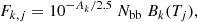
We used the SS data from four regular outbursts to determine the extinction AV toward the source. We selected 236 nights, during which GX 339-4 was observed in all four ONIR filters. We converted magnitudes to fluxes using the zero points given in Buxton et al. (2012, see also Table 3). Assuming that the SS spectra can be described by the blackbody model, we fit the data with the diluted Planck function modified by the interstellar extinction as follows:
 (1)
(1)
ONIR filter effective wavelengths λ, zero-point fluxes F0 (Buxton et al. 2012) and derived extinction.
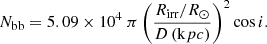
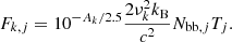
where k corresponds to one of the ONIR filters (V, I, J, H), index j corresponds to the date, Fk, j is the model flux (in mJy), Bk is the value of the Planck function at the effective frequency of filter k, Tj is the estimated blackbody temperature, and Ak is the extinction (in magnitudes) in k-filter obtained using the model of Cardelli et al. (1989) with correction by O’Donnell (1994). The dimensionless normalization Nbb is assumed to be the same for all outbursts. It can be expressed through the effective radius of the irradiated disk Rirr, the distance to the source D, and the disk inclination i as
 (2)
(2)
We noticed that the fluxes in the I filter are systematically offset from the blackbody fits for any AV. This might be caused by the deviation of the irradiated disk spectrum from a simple black body. Therefore, for fitting purposes, we introduced a correction ΔAI to the extinction in the I filter as an additional parameter. The best-fit parameters estimated using Bayesian inference are AV = 3.58 ± 0.02 mag, ΔAI = 0.15 ± 0.02 mag, and log10Nbb = 4.09 ± 0.01. Figure 3 shows the joint posterior distribution of the fitted AV and Nbb.
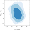 |
Fig. 3. Joint posterior distribution of the model parameters. Contours correspond to 0.68, 0.95, and 0.99 probabilities. |
Extinction can also be estimated using the color excess EB−V. The value EB−V = 0.94 ± 0.19 mag was derived from the X-ray absorption by Homan et al. (2005), while Zdziarski et al. (1998) give EB−V = 1.2 ± 0.1 mag as a weighted mean obtained from different methods. Using interstellar absorption lines, Buxton & Vennes (2003) got EB−V = 1.1 ± 0.2 mag. These extinction estimates correspond to AV between 2.9 and 3.7 mag (assuming RV = 3.1, Cardelli et al. 1989). Thus, our estimate of AV is well within the range of previously used values.
Our assumption that the blackbody normalization remains the same for all outbursts can be violated. For example, the effective disk radius in the LMXB XTE J1859+226 decreased with decreasing disk temperature (Hynes et al. 2002). It is unclear whether this happens as a consequence of the changes in the geometrical size of the disk or disk warping, or because of the propagation of the cooling wave (King & Ritter 1998). GX 339-4 shows complex behavior in its soft states (see Sect. 3.4 for the discussion), so it is possible that the normalization is indeed variable, which can systematically offset the inferred value of AV. To address this issue we tried to fit Tj and Nbb, j individually for each night, where AV and ΔAI remain global parameters. This problem is numerically unstable because in the Rayleigh-Jeans regime (i.e., at high temperatures) Eq. (1) transforms into
 (3)
(3)
As a result, contributions of Nbb, j and Tj cannot be easily decoupled and observations at higher energies (e.g., in UV) are required to properly fit temperatures and normalizations.
We also investigated the influence of the variable effective radius Rirr on the fitted value of AV by introducing different normalizations for each outburst. We find no evidence that the variation in the normalization significantly affects the inferred value of AV.
Using the obtained value of the blackbody normalization Nbb we now estimate the characteristic size of the accretion disk. From the distance and inclination of the binary system given in Table 4, we obtain Rirr = (3.0±1.1) R⊙. We then estimate the binary separation  (see, e.g., Frank et al. 2002), size of the primary Roche lobe RL, 1/a = 0.49/[0.6+q2/3log(1+q−1/3)] (Eggleton 1983), and the maximum disk size due to the tidal instability Rtidal/a = 0.60/(1 + q) (Paczynski 1977; Warner 1995). This allows us to compare the parameters of GX 339-4 to its “twin” system XTE J1550-564 (Muñoz-Darias et al. 2008).
Parameters of the system.
Analysis of the ONIR light curves of the 2000 outburst of XTE J1550-564 (Poutanen et al. 2014) showed that the effective radius of the irradiated disk of XTE J1550-564, Rirr ≈ 4.1 R⊙, is 40% smaller than the maximum disk size of 6.9 R⊙. Although GX 339-4 and XTE J1550-564 binary systems have similar sizes (Orosz et al. 2011; Hynes et al. 2003b; Heida et al. 2017), the major difference is the binary mass ratio q, which is on the order of 0.033 for XTE J1550-564 and 0.18 for GX 339-4 (see Table 4). A larger mass ratio leads to a smaller primary Roche lobe size, limiting the maximum size of the accretion disk.
3.3. Outburst template
In this section we study the V − (V − H) CMD of the regular outbursts to construct the outburst template. We use data from a given phase (RPh, RHS, SS, DHS, and DPh) to compute the 90 percent density contour with the exception of the 2004–2005 outburst, whose RHS we omit because it is systematically fainter than that of the other regular outbursts. The obtained template is shown in Fig. 4 and we further use it to study the similarities between regular outbursts and the peculiarities of the failed outbursts.
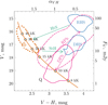 |
Fig. 4. Evolution of magnitudes and colors of GX 339-4 throughout the outburst. V and V − H are observed magnitudes and colors, FV is corrected for the interstellar extinction flux, and αVH is the intrinsic spectral slope, computed assuming AV = 3.58 mag (see Eq. (5)). The dashed pink contour corresponds to the RPh, the top right solid blue contour represents the RHS, the top solid green arrow indicates the HtS transition, dotted orange contour corresponds to the SS, the bottom solid green arrow represents the reverse StH transition, the bottom solid blue contour indicates the DHS, and the solid pink contour corresponds to the DPh. The solid orange line gives the model blackbody curve with log10Nbb = 4.09, see Eq. (1) and the filled blue diamonds along the curve correspond to the temperatures marked on the right. The quiescent state is denoted with letter Q in the lower part of the diagram. |
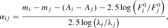
We compute the intrinsic spectral slopes αij, where the flux depends on frequency as Fν ∝ να, from the observed colors as
 (4)
(4)
where i, j correspond to ONIR filters (V, I, J or H), mi − mj is the observed color, Ai and Aj are the interstellar extinctions, λi and λj are the effective wavelengths, and  and
and  are the zero-point fluxes in i and j filters, respectively (see Table 3). Equation (4) for V and H filters can be reduced to
 (5)
(5)
The observed RPh begins with the spectrum resembling black body with temperature T ≈ 14 kK. The spectrum then reddens as it enters the RHS, reaching V − H ≈ 4 mag. During the HtS transition which takes 5–10 d, the spectrum becomes bluer. This evolution may be attributed to the quenching of the red nonthermal component. In the SS the source moves along the blackbody track (see Fig. 4, solid orange curve) toward top left part of the CMD, indicating a temperature increase from roughly 30 up to 50 kK. In 100–200 d, ONIR fluxes decrease and the temperature drops substantially. This marks the end of the SS and the beginning of the StH transition, which occurs at T ≈ 20 kK. The StH transition takes 11–18 d and the source moves almost horizontally on the V − (V − H) CMD, indicating an increase of flux in H filter at almost no changes in V. GX 339-4 spends 20–30 d in the DHS (although, in 2007 it lasted for more than 100 d) and after that it enters the DPh. During the next ∼50 d, the observed ONIR fluxes drop dramatically and the spectra become bluer. The Q phase does not follow the blackbody track and shows a substantial (up to 1.5 mag) variability of V − H color, unlike in other systems (see Kalemci et al. 2013; Poutanen et al. 2014).
We find that the colors and magnitudes of RHS are systematically different from those of DHS. The RPh is somewhat bluer than the DPh for the same V magnitude (Fig. 4). The SS contour is elongated along the blackbody track, but there is some spread of the data points around the model. This is likely caused by the variability due to superhumps (Kosenkov & Veledina 2018).
The spread of colors in the Q phase is peculiar. It cannot be explained by the measurement errors (see Fig. 5a, bottom left corner), as this spread exceeds the typical error by a factor of 10. Interestingly, most of the Q-phase data points lie below the blackbody line, that is, the colors are typically bluer than the black body that has the same V flux. We also note that the lowest observed blackbody temperature when the source enters the Q-phase is still above the hydrogen ionization limit.
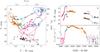 |
Fig. 5. Panel a: V versus V − H CMD of the 2002–2003 outburst. The filled upward-facing pink triangles correspond to the RPh, the filled blue circles indicate the RHS, the filled downward-facing green triangles represent the HtS transition, the filled orange squares indicate the SS, the open upward-facing green triangles correspond to the StH transition, the open blue circles indicate the DHS, the open downward-facing pink triangles correspond to the DPh, and the black crosses indicate the Q. Contours are the same as in Fig. 4. The typical 1σ errors are shown in the bottom left corner: the top orange cross corresponds to the bright states and is comparable to the plot symbol size; the bottom black cross corresponds to the quiescent state data, where observational errors are substantial. Panel b: ONIR H (top) and V (bottom) light curves of the same outburst. Symbols are the same as in panel a. Errors are 1σ and error bars are comparable to the symbols size. The solid black line represents the model, fitted to the part of the SS data. The gray area around the line denotes 1σ errors and also includes the contribution from the intrinsic scatter. Panel c: ASM A X-ray light curve. |
3.4. Regular outbursts
In this section we describe the properties of each outburst. We stress the peculiarities and deviations from the common pattern discussed above. The 2002–2003 outburst is the only one with many observations of the initial RPh (Fig. 5). This outburst was also observed during the HtS transition. Thus, we can trace the evolution of GX 339-4 before and after the RHS and compare it to the decay stages: StH transition, DHS, and DPh. Interestingly, after the HtS transition, the flux in H filter showed no visible variability in the daily timescale (see Fig. 5b; also Homan et al. 2005). In about 40 d (MJD 52440), when the flux started to decrease, the variability, which was previously attributed to superhumps (Kosenkov & Veledina 2018), became apparent. At the time of this change, the ASM fluxes and ASM B/A hardness ratio had a local minimum (see Fig. 5b,c).
The 2004–2005 outburst was fainter, both in the X-rays and in ONIR, as compared to other regular outbursts (see Figs. 1 and 2). The same conclusion can be reached from Fig. 6a, in which the RHS are located between two template (RHS and DHS) contours. The duration of the RHS, ≈180 d, is longer than that in the other outbursts (20–75 d). The V-filter flux increased after the transition to SS, and then decreased together with the decreasing ASM fluxes (Figs. 6b,c). The DHS points are located well within the template contour, and the corresponding fluxes are only marginally lower than those of the RHS, in contrast to other regular outbursts.
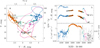 |
Fig. 6. Same as Fig. 5, but for the 2004–2005 outburst. Panel c: the BAT data are shown with open gray squares starting from the second half of the 2004–2005 outburst. Errors are 1σ. |
The 2007 outburst demonstrates unusually short SS and a long DHS. Both ASM and ONIR fluxes decayed after the HtS transition (Figs. 7b,c), and the decay took about 100 d, as compared to typical 250–300 d for other outbursts. On the contrary, the DHS lasted over 100 d in contrast to typical ∼50 d for other outbursts. It is even possible that this phase continues throughout the first half of 2008.
The ONIR light curves of the 2010–2011 outburst show a peculiar trend discontinuity during the SS (around MJD 55360, see Fig. 8b). Nevertheless, all SS data points align well with the blackbody model on the CMD (Fig. 8a); hence, the observed break is caused by a sudden decrease in the color disk temperature.
3.5. Failed outbursts
There are three failed outbursts in 2002–2011, in 2006 (see Figs. 9), in 2008 (see Fig. 10) and in 2009 (see Fig. 11), when GX 339-4 does not enter the SS, in contrast to regular outbursts. The ONIR peak fluxes are a few times smaller than the RHS of regular outbursts, however, the colors are the same. The duration of different phases of failed outbursts is comparable to those of regular outbursts.
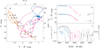 |
Fig. 9. Same as Fig. 6, but for the 2006 failed outburst. Blue circles indicate the bright phase of the outburst and black crosses indicate the quiescent state. The transition is shown with pink triangles. |
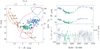 |
Fig. 10. Same as Fig. 9, but for the 2008 failed outburst. Filled green triangles indicate the transition from the initial bright phase to the faint phase and open green triangles show the rebrightening. |
The 2006 and 2009 failed outbursts have similar duration and peak magnitudes. The light curves of the 2009 failed outburst have a double-peaked profile (both in the ONIR and X-rays) and the V − H colors of both peaks are the same. Interestingly though, the brightest episode of the 2009 outburst resembles the RHS of the 2004–2005 regular outburst in terms of phase duration, typical ONIR magnitudes, and colors (compare Fig. 6b and Fig. 11b, blue dots). This similarity makes it harder to distinguish between regular and failed outbursts at early phases.
The 2008 failed outburst peak is about 0.5 magnitude fainter than that of the other failed outbursts. It consists of two peaks (Russell et al. 2008; Kong 2008), both of which have colors and magnitudes typical of the DHS (see Fig. 10a). The second brightening is, on the other hand, considerably longer than the typical DHS. Between the two peaks the source dims and becomes bluer as if it were going to the SS, similar to the HtS transition. However, it reddens again and returns back to the DHS along a similar track on the CMD. Therefore, we color these phases on the CMD as HtS and StH. We note that the timescales are somewhat larger (40–50 d as opposed to 10–20 d; see Fig. 10b, Table 2). Although we consider the 2008 outburst as a separate event, there is a possibility that it could be a continuation of the exceptionally long 2007 outburst.
We note that the distinction between the failed and regular outbursts is not possible from the ONIR data alone at their earlier stages. However, it might be possible using the peak V magnitude. If the source is brighter that V = 16 mag during the RHS, it transits to the SS. On the other hand, if it is fainter, the outburst can be either regular (2004–2005 outburst, see Fig. 6) or failed (2009 outburst, see Fig. 11).
3.6. Evolution of the nonthermal component
It is known that changes in ONIR colors during the HtS and StH transitions are related to the quenching or recovery of the red, nonthermal component (see, e.g., Fender et al. 1999; Jain et al. 2001; Corbel & Fender 2002). To understand the origin of the nonthermal emission, it is important to obtain a reliable estimate of its spectral shape by subtracting the contribution of the thermal (disk) component. The task is, however, complicated by the fact that the spectrum of the thermal component (e.g., disk temperature) is an unknown function of time. The spectral index of the nonthermal component may allow us to distinguish between two alternatives: the jet (Fender 2001; Gallo et al. 2007; Uttley & Casella 2014) and the hot flow (Veledina et al. 2013; Poutanen & Veledina 2014; Kajava et al. 2016). The contribution of the disk can be estimated by fitting the SS light curves in different filters, and extrapolating the obtained fit to the transitions and the hard state (see, e.g., Buxton et al. 2012; Dinçer et al. 2012; Poutanen et al. 2014). The weakness of this approach is related to freedom in the choice of the fitting function and fitting interval, which leads to an uncertainty in the spectrum of the nonthermal component.
In general, the emission of the irradiated accretion disk is expected to follow the fast rise – exponential decay profile (and a constant level of emission in quiescence; see, e.g., Chen et al. 1997). The exponential decay profile was fit to the 2000 outburst data of XTE J1550-564 (Poutanen et al. 2014), while GX 339-4 shows both episodes of decay and rise during the SS. Therefore, we fit parts of the SS light curves using the following model:
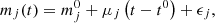 (6)
(6)
where μj is the slope, which can be positive or negative. In this equation, mj is the observed magnitude in jth ONIR filter,  is the constant, t is the time, t0 is either the beginning (if the fitted data set covers the first part of the SS) or the end time of the fitted data set (if it covers the last part of the SS), and ϵj is the intrinsic scatter, which is partially caused by superhump variability (Dinçer et al. 2012; Kosenkov & Veledina 2018). We use Bayesian inference to estimate these parameters and list these in Table 5.
Once the fit to the SS is obtained, we extrapolate the model for 30 days from the start or the end of the SS, which usually covers the transition phase and a part of the hard state. The errors on the fluxes of the nonthermal component are mostly coming from the uncertainties in the parameters of the fitted model and they increase toward the hard state. In contrast, the contribution of the disk also drops and it falls down to about 5% in the RHS.
The fitted models are shown in Figs. 5–8(b) with solid black lines. The gray areas around the model denote 1σ uncertainties. The model curve spans over the SS data used for fitting, the transition phase (if present) up to the nearest hard state. The total spectra and the spectra of the nonthermal component are shown in Fig. 12. The fluxes are corrected for the interstellar extinction assuming AV = 3.58 mag (see Sect. 3.2).
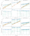 |
Fig. 12. Sample of spectra from the soft state (orange squares), transition (green triangles), and the hard-state spectra (blue circles). The open symbols represent the StH state transitions, while the filled symbols indicate the HtS state transitions. Top panels (a–f): total observed spectra of the decaying part of the 2002–2003 outburst, the rising and decaying parts of the 2004–2005 outburst, the 2007 outburst, and the rising and decaying parts of the 2010–2011 outburst, respectively. Bottom panels (a*–f*): corresponding spectra after subtraction of the thermal component. Fluxes are corrected for the interstellar extinction; errors are 1σ. |
In the majority of cases, both the hard state and the state transition spectra of the nonthermal component appear to be nearly flat (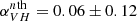 ); the best examples are the 2004–2005 DHS and 2010–2011 RHS (see Figs. 12c*,e*). During the transitions, the spectral shape of the nonthermal component is stable. We also note that there is no apparent difference between spectral shapes of that component in the StH and HtS transitions.
The spectral slope αONIR is affected by the assumed value of AV. The impact of AV can be estimated using Eq. (5). For a relatively low value of AV ≈ 3.0 mag (Kong et al. 2000; Homan et al. 2005),  , while for a relatively high AV = 3.7 mag (Zdziarski et al. 1998; Buxton et al. 2012) we get
  . The changes in AV are also reflected in the curvature of the blackbody track on the CMD located within the SS contour (see discussion in Sect. 4.1).
To illustrate the results of our spectral decomposition, we selected a sample of the RHS, HtS, SS, StH and DHS data of each regular outburst. We fit a model consisting of a power law of index α = 0 to account for the nonthermal component (except for the SS) and a blackbody to the data corrected for the interstellar extinction. The blackbody normalization is allowed to vary between the outbursts. The results are shown in Fig. 13. This simple model reproduces the data very well.
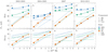 |
Fig. 13. Selected spectra of the rising (top panels) and decaying (bottom panels) stages of regular outbursts. The 1σ errors are comparable to the symbol size. The solid orange and dotted blue and green lines correspond to the blackbody (BB) component in the soft and hard states and transitions, respectively. The dashed blue and green lines correspond to the power-law spectra of the hot flow (HF). The solid lines give the sums of the corresponding blackbody and the hot flow components. In panel b the HtS spectrum is not plotted because there are no observations with simultaneous measurements in three or more ONIR filters. Instead, two RHS spectra are shown, separated by ∼150 d, to highlight the evolution of both nonthermal and disk components (see also Fig. 6). |
3.7. Broadband spectra in the hard state
The hard-state mid-IR spectra of GX 339-4 can help us identify the nature of the nonthermal component. GX 339-4 was observed in the mid-IR with WISE on MJD 55265.88–55266.88 (Gandhi et al. 2011). The 13 mid-IR spectra can be divided into two groups. At lower fluxes, the WISE spectra are nearly flat (see spectra #1, 2, 7, and 8 in their Fig. 3) and lie on the continuation of the ONIR nonthermal component. At higher fluxes, the spectra are much softer and most have a large curvature (e.g., spectra #3–6, 9, 12–13; see also blue triangles in Fig. 14).
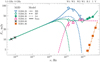 |
Fig. 14. Broadband spectra of GX 339-4 using the radio ATCA, mid-IR WISE, and ONIR SMARTS data. The figure shows four distinct spectral shapes for the source. The orange squares show the soft-state data from MJD 55301.36, the filled green circles and open green diamonds indicate the quasi-simultaneous ONIR and mid-IR data on MJD 55266.35. The open blue downward-facing triangles and open pink upward facing triangles show the mid-IR spectra measured 1.7 h before and after the quasi-simultaneous observation, respectively. The black crosses indicate one of the closest available ATCA radio observations (MJD 55269.80) that is used to constrain the jet properties. The lines show different model components: the dot-dashed orange line indicates the blackbody component, the dashed pink line shows the hot flow component, the dotted lines correspond to the jet model with different cutoff frequencies, and the solid lines give the sum of the three (blackbody + hot flow + jet) components. The sum of the blackbody and hot flow components for MJD 55266.41 is not shown for convenience because it fully coincides with the hot flow curve in the mid-IR. The 1σ errors are comparable with the symbol size. The WISE fluxes are adjusted by the normalization factors inferred from the fit (see Table 6). |
The source shows strong variability, by a factor of three, in all four WISE filters on the timescales of hours (see Fig. 2a and Table 1 in Gandhi et al. 2011). The variability amplitude increases toward longer wavelengths. Extrapolation of the WISE spectra to the ONIR bands predict an order of magnitude variation there. However, the observed ONIR nonthermal component is nearly constant. This suggests that there are two nonthermal components: one that is highly variable dominating during high mid-IR flux episodes and another, more stable, emitting in a broad range from mid-IR to ONIR. There is a caveat though that the typical WISE exposure is about 10 s, which is much smaller than the typical 300 s exposure in the ONIR bands.
To understand the nature of these components, we tried to construct the broadband spectra of the source. All available 13 WISE observations occurred during 24 hours on MJD 55265.9–55266.9. There is one observation on MJD 55266.3481, which is just 16 min before the SMARTS observations on MJD 55266.3594. In addition we also chose the two nearest WISE observations 1.7 h before and after the quasi-simultaneous observation on MJD 55266.28 and on 55266.41. In order to estimate contribution from the disk blackbody, we used the SS ONIR observation on MJD 55301.36 because the ONIR flux was nearly constant after the HtS transition (see Fig. 8). Furthermore, we selected the closest in time ATCA 5.5 and 9 GHz measurements obtained on MJD 55269.80 (Corbel et al. 2013a). Albeit the radio and mid-IR data are taken on different dates, the extrapolation of the hard radio spectrum matches the high-flux WISE data. The connection between the radio and mid-IR fluxes and their high variability on short timescales are hallmarks of the jet emission as seen in blazars (Tavecchio 2017; Zacharias 2018). The simple jet model of Blandford & Königl (1979), which was often invoked to explain the radio to near-infrared spectra of GX 339-4 (see, e.g., Corbel & Fender 2002; Gandhi et al. 2011; Rahoui et al. 2012; Corbel et al. 2013b), does not address the presence of the sharp cutoff in the mid-IR spectra and the dichotomy of mid-IR spectral slopes.
We suggest that the broadband spectrum of GX 339-4 consists of (at least) three components. We model the disk component by the blackbody. We use a power law with spectral index close to zero, which transforms to Rayleigh-Jeans spectrum at lower-frequencies, to model the hot flow. The jet is described by a power law with a high-frequency cutoff. The model can be described by the following equations:
![Mathematical equation: $$ \begin{aligned} \begin{aligned}&F_\nu ^\mathrm{bb} = N_{\rm bb}\ B_\nu (T),\\&F_\nu ^\mathrm{hf} = N_{\rm hf} \left(\frac{\nu }{10^{14}\,\mathrm{Hz}}\right) ^ \alpha \left\{ 1 - \exp \left[ - \left( \frac{\nu }{\nu _{\rm hf}} \right)^{2-\alpha } \right] \right\} , \\&F_\nu ^\mathrm{jet} = N_{\rm jet} \left(\frac{\nu }{10^{10}\,\mathrm{Hz}}\right) ^ \beta \exp \left[ -\left(\frac{\nu }{\nu _{\rm jet}}\right)^\gamma \right],\\&F_\nu ^\mathrm{tot} = F_\nu ^\mathrm{bb} + F_\nu ^\mathrm{hf} + F_\nu ^\mathrm{jet} , \end{aligned} \end{aligned} $$](/articles/aa/full_html/2020/06/aa36143-19/aa36143-19-eq15.gif) (7)
(7)
where  ,
,  ,
,  , and
, and  are the model fluxes of the disk, hot flow, jet components, and their sum, respectively, Nbb, Nhf, and Njet are the model normalizations, T is the blackbody temperature, νhf is the low-frequency cutoff of the hot flow component, νjet is the high-frequency cutoff of the jet spectrum, α and β are the corresponding power-law slopes, and γ is the index of the super-exponential cutoff. The value of log Nbb is fixed at 4.09 derived in Sect. 3.2.
Figure 14 shows the RHS spectra of GX 339-4 as observed by ATCA, WISE, and SMARTS together with one SS ONIR spectrum as well as the best-fit models. We assume that the hot flow spectrum is the same for all three mid-IR spectra. For the jet component, we use different cutoff frequencies because normalization and power-law slope are determined by the shape of the radio data, which is the same in all cases. Owing to the difference in the exposure times of WISE (<10 s) and SMARTS (300 s) and some systematic uncertainties in the absolute flux of WISE, we apply additional cross-calibration factor to the mid-IR fluxes, which is treated as a free parameter. The best-fit parameters are given in Table 6.
We see that on MJD 55266.28 the jet outshines the hot flow by a factor of 2–3 in W4 and W3 filters. The overall radio to ONIR spectrum cannot be described by a broken power law plus a black body. This implies that the spectrum above ∼3 × 10¹³ Hz is not consistent with an optically thin, power-law-like synchrotron spectrum predicted by a standard jet model of Blandford & Königl (1979). The sharp cutoff below 1014 Hz cannot be described even by a simple exponential cutoff, but is well fit only by a super-exponential with the index γ ≈ 2. If we interpret the power-law spectrum from radio to the mid-IR as a combination of self-absorbed synchrotron peaks, such a cutoff can only be obtained if the electron distribution producing the mid-IR emission has a very steep slope.
On MJD 55266.35 the jet likely contributes to the W4 filter, but the hot flow takes over at higher frequencies. The WISE spectrum obtained on MJD 55266.41 is the hardest spectrum with α = 0.16 having a clear curvature below 2 × 10¹³ Hz, which can be associated with the synchrotron self-absorption frequency of the hot flow spectrum (dashed pink line). Therefore the hot flow likely dominates in all mid-IR filters and contributes to the ONIR flux together with blackbody component. The measurement of the low-frequency cutoff allows us to constrain the size of the hot flow (corona) to be (Eq. (13) in Veledina et al. 2013) Rhf ≈ 3 × 10⁹ (1013 Hz/νhf) ≈ 2.7 × 109 cm, which corresponds to 900 Schwarzschild radii for a 10 solar-mass BH. For this observation, we obtain only an upper limit on the jet cutoff frequency because the contribution of the jet to the mid-IR is negligible.
4. Discussion
4.1. ONIR spectra
The magnitude-magnitude diagrams (see Buxton et al. 2012) can be used to emphasize the difference between hard and soft states and to highlight the state transition tracks. However, these diagrams do not provide sufficient information about the shape of the spectra in each of the observed states and make it harder to separate RHS and DHS data points as they roughly follow the same broken power-law track (together with the data from quiescence; see, e.g., Fig. 9 in Buxton et al. 2012). Alternatively, we can use CMDs (Maitra & Bailyn 2008; Russell et al. 2011; Poutanen et al. 2014). The benifit of CMD plots is that they highlight both changes in the observed fluxes and shape of the spectra. The characteristic hysteresis pattern tracked by the source on the CMD can be related to the hysteresis observed in the X-ray data (Poutanen et al. 2014). In three out of four regular outbursts, GX 339-4 was observed to have nearly identical HtS and StH transitions patterns on a CMD (see Sect. 4.2 for a discussion; also Fig. 1 in Corbel et al. 2013a, Fig. 1 in Muñoz-Darias et al. 2008), while during the HtS transition of the rising phase of the 2002–2003 outburst the X-ray fluxes were a few times smaller than the typical values (Figs. 2b,c). Interestingly, even though the 2002–2003 HtS transition starts at lower ONIR fluxes, it arrives at the same SS flux with a color temperature of 30–35 kK.
Recently, the CMD was used to study the spectral evolution of the BH X-ray binary XTE J1550-564 during its 2000 outburst (Poutanen et al. 2014), which was very similar to that of GX 339-4. Notably, the highest SS disk temperature of 16 kK reached by XTE J1550-564 is substantially smaller than the temperature of 50 kK in GX 339-4 (see Fig. 8). The inferred SS temperatures can be affected if AV is overestimated. We note, however, that for a lower AV the disk temperature becomes smaller, leading to a different curvature of the blackbody track on the CMD, which is inconsistent with the observed shape drawn by the SS data points (see Fig. 4, solid orange line and dotted orange contour). Furthermore, the UV observations of GX 339-4 carried out during the early phase of the 2010–2011 SS suggest that the peak of the blackbody component lies at wavelengths shorter than ≈2000 Å, beyond the near-UV (see Fig. 7 in Cadolle Bel et al. 2011), which imposes a lower limit of ≈15 kK on the blackbody temperature at the beginning of the SS. Unlike XTE J1550-564, which shows a typical exponential decay of ONIR fluxes during its SS, ONIR fluxes of GX 339-4 increase shortly after the HtS transition in two out of four regular outbursts. As a result, the highest color temperatures of GX 339-4 are observed somewhere in the middle of the SS, while the highest blackbody temperature of XTE J1550-564 is found at the beginning of the SS.
The disk temperatures depend on the flux irradiating the outer parts of the disk. This flux is defined by the disk geometry, luminosity of the central X-ray source, and its emission pattern, which in turn depends on the BH spin. The accretion disk in GX 339-4 can be a factor of ∼2 smaller than that in XTE J1550-564 (see Table 2; also Orosz et al. 2011). Geometrically thicker outer parts of the disk may also increase the amount of irradiation flux received. Then, the light bending effects in the vicinity of a Kerr BH substantially increase the intensity of the illuminating flux (Suleimanov et al. 2008). There is evidence that the BH spin of GX 339-4 can be as large as a ≈ 0.935 (Reis et al. 2008, Miller et al. 2008; but see also Kolehmainen & Done 2010; Kolehmainen et al. 2011 and Zdziarski et al. 2019 who give an upper limit of 0.8–0.9) compared to a ≈ 0.5 in XTE J1550-564 (Steiner et al. 2011). It is possible that a combination of these factors leads to a higher SS temperatures inferred in GX 339-4. Furthermore, the extinction in XTE J1550-564 assumed by Poutanen et al. (2014) might have been underestimated; a higher AV would result in a larger temperature bringing it closer to the values measured in GX 339-4.
The Q states of GX 339-4 appear to deviate from those observed in XTE J1550-564. While for XTE J1550-564 these points lie on the blackbody track, for GX 339-4 they lie below the blackbody curve. It is known that the contribution of the companion star is small even in quiescence (up to 50 per cent to the J and H filters, Heida et al. 2017), and the red spectrum of the K-type companion cannot explain the shift toward the blue part of the CMD, as well as the substantial variability of colors in GX 339-4 (Zdziarski et al. 2019). Other LMXBs are known to exhibit quiescent flickering, but the magnitude of quiescent variability of GX 339-4 and significant changes in observed colors exceed that measured for other sources (Zurita et al. 2003). A possible explanation for this behavior is the emission from the spiral arms, hotspots, and hot line flares triggered by the magnetic field reconnection in the vicinity of the disk, and the presence of edges and lines in the quiescent spectra (see, e.g., Zurita et al. 2003; Cherepashchuk et al. 2019; Baptista & Wojcikiewicz 2020).
We find that the regular and failed outbursts occupy the same regions in the CMD. Although the regular outbursts tend to be more luminous during the RHS, the position of the points of the 2004–2005 outburst intersects with brightest parts of the analyzed failed outbursts. We thus conclude that the peak ONIR brightness has no predictive power for the failed outbursts. The reason for the similarity of ONIR brightness of regular and failed outbursts is not clear from the light curve and CMD analysis. If the failed outbursts differ from the regular outbursts by the mass transfer rate, then the similar brightness during the RHS can be explained by a weak dependence of the nonthermal component on the accretion rate. Because it dominates in the ONIR, the difference between regular and faint outbursts is minor.
4.2. ONIR versus X-ray correlation
Black hole LMXBs show strong nonlinear correlation between radio, ONIR, and X-ray fluxes. The radio–X-ray correlation was first documented for Cyg X-1, GX 339-4 and V404 Cyg (Brocksopp et al. 1999; Corbel et al. 2000; Gallo et al. 2003) and later was confirmed on a much larger sample of Galactic LMXBs (including GX 339-4 during multiple outbursts; see Corbel et al. 2013a; Islam & Zdziarski 2018). The global ONIR–X-ray correlation, which naturally arises from the different emission mechanisms (van Paradijs & McClintock 1994; Gallo et al. 2003), was observed for a number of BH LMXBs (Russell et al. 2006) and for the 2002–2003, 2004–2005, and 2007 outbursts of GX 339-4, in particular (see Homan et al. 2005; Coriat et al. 2009). We expand the sample to include the 2010–2011 outburst.
We use the RXTE/ASM flux as a proxy for the X-ray luminosity. The observed flux, however, cannot be simply transformed into the bolometric luminosity, as the latter depends on the spectral shape. The bolometric correction is large in the hard state and the quiescence as most of the emission is radiated at energies above the ASM passband. We use the observed H-band flux as a proxy for the luminosity of the nonthermal component. Figure 15 shows the relation between the H-band and X-ray fluxes for the regular outbursts (see also Zdziarski et al. 2002). The source moves in the clockwise direction on this diagram, where the hysteresis pattern is similar to that found by Coriat et al. (2009).
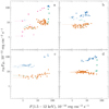 |
Fig. 15. Quasi-simultaneous ONIR νHFH vs. X-ray 1.5−12 keV flux diagram. The X-ray data are taken from all three ASM bands. The colors and symbols are the same as in Fig. 5 and errors are 1σ. 2002–2003 (panel a), 2004–2005 (b), 2007 (c), and 2010–2011 (d) outbursts. |
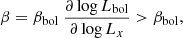
In the beginning of the SS, the H-band flux is nearly constant and has a hint of anti-correlation with the X-ray flux in the last outburst (Fig. 15d), which is likely caused by the changing bolometric correction. Such anti-correlation between ONIR and X-ray fluxes is atypical for GX 339-4 and other LMXBs, for which HS and SS correlations have very similar slopes (Figs. 15a,b,c; also Russell et al. 2006, 2007; Coriat et al. 2009). The RHS of the 2010–2011 outburst (Fig. 15d) seems to have a slope, which is not as steep as observed in other outbursts, where ∂ log(νHFH)/∂ log F(ASM) ≈ 0.3, as compared to ≈0.4 for the 2002–2003 and 2007 events.
The relation between ONIR and X-ray fluxes can be used to put constraints on the models of spectral formation in accreting BHs. The scaling of the ONIR and X-ray fluxes with the mass accretion rate was used to predict the observed ONIR – X-ray correlation in the jet-dominated scenario (Russell et al. 2006). We suggest an interpretation of the HS correlation in the framework of the hot accretion flow model (Veledina et al. 2013; Poutanen & Veledina 2014). The schematic representation of the spectrum in the ONIR–X-ray range is shown in Fig. 16. For a broken power-law spectrum, we can relate the ONIR (Lo) and X-ray (Lx) luminosities as
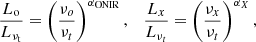 (8)
(8)
 |
Fig. 16. Schematic representation of the evolution of GX 339-4 spectra during the rising phase hard state and HtS transition of an outburst. The dotted pink line indicates the RPh hard spectrum, the solid blue line corresponds to the RHS, and the dashed green line represents the HtS transition. The vertical black arrows indicate the transition sequence. Characteristic turnover frequency of each spectrum and the V filter frequency are shown with the vertical dashed lines. Characteristic spectral slopes in the ONIR and X-ray ranges are shown with αONIR and αX. |
where νt is the (break) turnover frequency, αONIR and αX are spectral slopes, and νo and νx are characteristic frequencies in the ONIR and X-ray ranges, respectively. The ratio of the X-ray to ONIR luminosity is then
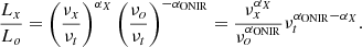 (9)
(9)
Therefore the slope of the optical–X-ray correlation is written as
 (10)
(10)
where β ≡ ∂ log νt/∂ log Lx.
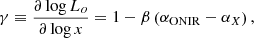
We take αX ≈ −0.7 and αONIR ≈ 0 (average of four regular outbursts, see Sect. 3 and Fig. 12). The turnover frequency scales with the magnetic field B and the Thomson optical depth τ across the flow as
 (11)
(11)
where p is the power-law slope of the electron distribution. Assuming density scaling with the accretion rate ρ ∝ ṁ (i.e., τ ∝ ṁ too) and equipartition magnetic field B2 ∝ ρ (assuming constant temperature), we arrive at
 (12)
(12)
The bolometric luminosity scales with the accretion rate as ṁ or as ṁ2 for the cases of hot, radiatively efficient (e.g., Bisnovatyi-Kogan & Lovelace 1997) or inefficient (advection-dominated) accretion flow (e.g., Narayan & Yi 1995), respectively. For these two cases we get
 (13)
(13)
Taking p = 4 to satisfy the slope of the MeV emission observed from Cyg X-1 (McConnell et al. 2002), we get βbol = 0.63 and 0.31 for the two cases. Assuming β = βbol we get γ ≈ 0.56 and 0.78, respectively. This range of γ is consistent with the observed slope of the optical–X-ray correlation γobs ≈ 0.6 obtained in Russell et al. (2006) for a number of BH LMXB sources. We observe γobs ≈ 0.4 (similar to γobs ≈ 0.48 in Coriat et al. 2009). Such slopes require β ≈ 0.8−0.9, which is hard to achieve. However, the underestimated value of γ can be caused by the variable bolometric correction. If it is positively correlated with the luminosity (see Zdziarski et al. 2004; Koljonen & Russell 2019)5 then
 (14)
(14)
bringing γ closer to the observed range.
4.3. Origin of the nonthermal ONIR component
The nature of the red nonthermal component seen in LMXBs during the ONIR flares is debated. Two main candidates are proposed: synchrotron emission from the jet or from the hybrid hot accretion flow (see reviews by Uttley & Casella 2014; Poutanen & Veledina 2014). In some cases the ONIR soft spectrum is consistent with the optically thin synchrotron emission and has been modeled with the jet (e.g., MAXI J1836-194; Russell et al. 2014; Péault et al. 2019). In other cases, when the disk-subtracted nonthermal component had a hard spectrum (Poutanen et al. 2014), or when the extrapolation of the radio continuum significantly underestimates ONIR fluxes (e.g., Swift J1753.5-0127; Chiang et al. 2010; Kajava et al. 2016), the excess ONIR emission has been attributed to the hot accretion flow. A way to discriminate between the two models is to track the behavior of nonthermal component during the ONIR state transition. In a simple jet scenario, the spectrum from radio to optical wavelengths can be described by a broken power law (Blandford & Königl 1979) that has partially absorbed and optically thin parts. During the HtS transition the synchrotron break frequency is expected to decrease, as it scales inversely proportional to the inner disk radius (Heinz & Sunyaev 2003). In the hot flow model, the spectrum from infrared to X-rays is expected to have two breaks: the lower-frequency break between the partially absorbed and fully self-absorbed parts (it corresponds to the extent of the flow), and the higher-frequency break between the partially absorbed and synchrotron Comptonization parts (Veledina et al. 2013). Under the simplest assumptions, the state transition is accompanied by the collapse of the flow outer parts, and so the lower-frequency break is expected to increase, while the spectral slope of the partially self-absorbed part can remain the same. The reverse trends are expected in the same scenarios for the StH transitions.
Unlike the expectations in these two simplest scenarios, we found that the nonthermal component has a constant spectral shape during the HtS and StH transitions, and only its normalization decreases (see bottom panels in Fig. 12). We propose that the aforementioned evolution can be understood in terms of the hot flow model, if both the energy release and the electron number density increase when the accretion rate increases during RPh. This then leads to an increase of total luminosity and an increase of a higher break frequency. As the accretion rate increases, the synchrotron emission, produced at the same physical radius in the flow, would shift to higher frequencies (as the frequency of self-absorption increases) and become brighter; see changes between dotted and solid lines and between turnover frequencies νt, 1 and νt, 2 in Fig. 16. In this model, the RHS is described by the increase of ONIR luminosity with a nearly constant spectral shape because the latter is determined by the distribution of parameters over the radius, rather than by their absolute values. At the HtS transition, when the energy release is shifting from the hot accretion flow to the geometrically thin accretion disk, the energy deposited in the hot flow decreases, while the particle density may still increase. This results in a higher break frequency, but smaller overall ONIR luminosity; see changes between solid and dashed lines and between turnover frequencies νt, 2 and νt, 3 in Fig. 16.
The hot flow model is capable of explaining both (nearly) constant colors of the nonthermal component during the RHS and the constant spectral shape at decreasing ONIR luminosity during the HtS state transition if the extent of the hot flow during the observed transitions has not decreased. This would guarantee that the emission in the H filter appears in the partially self-absorbed part. Thus in contrast to the expectations of the original scenario, the data can be described by the hot flow model if there is no collapse of the outer parts of the flow. We suggest that the survival of the synchrotron-emitting plasma with the inward-moving inner edge of the disk can be seen as the transition from the hot flow (within the boundaries of the cold disk) to the corona atop the accretion disk. This scenario is supported by the StH transition and the DHS, where we observe the same evolution happening in reverse. During the StH the spectra are nearly flat and their shapes do not change (see Figs. 12a*,c*,d*,f*), indicating that the H filter remains in the self-absorbed part and we observe a reverse process of transition from the hot corona atop of the disk to the hot flow, as the inner edge of the disk moves outward.
The shape of the ONIR spectra in the simplest jet scenario depends on the break frequency, which may lie beyond the V band (> 5 × 10¹⁴ Hz, see Coriat et al. 2009; Dinçer et al. 2012; Buxton et al. 2012) or in the mid-IR (1013−14 Hz; see, e.g., Corbel & Fender 2002; Gandhi et al. 2011). The problem is that estimates of the break frequency were obtained for different outbursts using different estimates for the extinction (see Homan et al. 2005, Maitra et al. 2009, and Buxton et al. 2012). In our interpretation of the quasi-simultaneous, mid-IR data obtained with WISE (Gandhi et al. 2011), there is likely another highly variable soft nonthermal component, which contributes to the mid-IR in addition to the power law. GX 339-4 shows two distinct mid-IR spectral shapes: a low-flux flat spectrum, which agrees with the power-law-like, disk-subtracted ONIR spectrum, and a high-flux soft spectrum, which drops sharply between W1 and H filters (see Fig. 14). If we interpret this additional soft component as coming from the jet, the jet break frequency is about 1014 Hz (see Table 6). This implies that the jet can dominate mid-IR fluxes, but as soon as the jet spectral slope (as determined from the radio data) changes to negative, the hot flow becomes the dominant source of the mid-IR emission, providing a baseline flux level in the mid-IR and ONIR filters. The shape and evolution of the ONIR spectra are then determined by the sum of the thermal disk and flat hot flow components with little to no contribution from the jet.
The fast variability observed in GX 339-4 can shed more light on the nature of the ONIR emission. Within the hot flow model, two components contribute to the variability in ONIR: synchrotron emission from the hot flow and reprocessing of the X-rays in the accretion disk. In this model (Veledina et al. 2011), a precognition dip in the optical–X-ray CCF is explained by anti-correlation of the ONIR synchrotron and the X-ray Comptonization components. The reprocessing produces a positive peak at positive lags. Together they can produce a typical CCF observed in many BH X-ray binaries (see Poutanen & Veledina 2014) including GX 339-4 (Gandhi et al. 2008, 2010). The IR versus X-ray correlation, however, appears to depend on the type and phase of the outburst. The CCF obtained for the 2008 failed outburst (low-flux hard state) shows no precognition dip and only a slight asymmetry (Casella et al. 2010), while CCF of the RHS of the 2010–2011 outburst features a precognition dip (Kalamkar et al. 2016). Although it is possible to explain this behavior within jet-only paradigm (see, e.g., Malzac et al. 2018), it is likely that both jet and accretion flow produce different features of the IR versus X-ray CCF (see also Sect. 3.7).
5. Conclusions
We analyzed the 2002–2011 ONIR light curves of GX 339-4. We used the ONIR data to separate the states of the source and compared the estimated transition dates with those obtained from the X-ray spectra. We measured the typical durations of various outburst stages: the HtS state transitions take typically a week, while the StH state transitions last twice longer. The duration of the hard state at the decaying stage is about four weeks.
Using the SS data from four regular outbursts, we determined the interstellar extinction toward the source, which allowed us to measure the intrinsic ONIR spectral slopes during different phases of the outbursts. We showed that during the outbursts the source passes through the same areas on the CMD, giving us an opportunity of constructing a template in which different outburst phases are identified.
During the SS, the object is found to follow the blackbody model with a constant normalization. During the HS, a red nonthermal component dominates the H band, where the flux is higher at the rising phase than at the decaying phase. We find that the end of the HtS transitions corresponds to the blackbody temperature of 30–40 kK, while at the start of the reverse transition the temperature is ≈20 kK. In quiescence, the spectrum of GX 339-4 is bluer than the blackbody model with the same normalization, which can be explained either by the presence of strong spectral features (edges) or by the decrease of the apparent emitting area. The corresponding disk temperatures are well above the hydrogen ionization limit. The variability of the source in this state exceeds the measurements errors and its nature is uncertain.
We traced the evolutionary tracks of the failed outbursts on the CMD and found that their HS show the same colors as the HS of regular outbursts, but lower ONIR fluxes. The decay of a failed outburst follows the same track as the decaying phase of a regular outburst. These properties make it difficult to predict the failed outburst at early stages using ONIR data alone. We found that a bright RHS, V < 16 mag, is a sign of a regular outburst.
Finally, we investigated the behavior of the nonthermal component, which dominates the ONIR fluxes during the HS and the state transitions. For this, we subtracted the contribution of the thermal component (disk) using the extrapolated SS light curves. We found that the luminosity of the nonthermal component evolves with a nearly constant power-law spectrum with energy spectral index α ≈ 0 (where Fν ∝ να). We proposed that this evolution can be explained by a model in which the nonthermal component originates from the synchrotron emission of the hot accretion flow. However, for this model to work, the extent of the hot medium should not decrease at the state transitions, but instead the hot flow should transforms into the hot corona atop of the accretion disk as the inner disk radius moves inward during the HtS transition. In this case, the H-filter remains in the partially self-absorbed region implying constant spectral shape. The reverse process may occur during the StH transition. Using radio ATCA and mid-IR WISE data contemporaneous with the available SMARTS data, we also showed that an additional strongly variable component, which is likely associated with the jet, is required in the mid-IR band. The spectrum of this component has a sharp cutoff below 1014 Hz. We also detected a low-frequency cutoff in the hot flow component at ∼1013 Hz, which can be used to estimate its size of about 3 × 109 cm. We conclude that at least three components (the disk, hot flow, and jet) are required to explain the broadband mid-IR to ONIR spectra of GX 339-4 at different stages of its outburst.
The data mentioned in the original publication (Buxton et al. 2012) cover the 2002–2010 period and the fluxes in I filter are computed using an incorrect extinction AI.
We note that bolometric correction can increase toward lower luminosities because the rising electron temperature (Veledina et al. 2013) results in a larger fraction of flux to emerge above 200 keV as well as in the ONIR band.
Acknowledgments
We thank the anonymous referees for valuable comments and suggestions, which helped improve the manuscript. AV acknowledges support from the Academy of Finland Grant 309308. VFS was supported by the DFG Grant WE 1312/51-1, the German Academic Exchange Service (DAAD) travel Grants 57405000 and 57525212 and by the Magnus Ehrnrooth Foundation travel Grant. This research was also supported by the Academy of Finland travel Grants 317552 and 331951 (IAK, JP). This paper has made use of SMARTS ONIR light curves. AV thanks the International Space Science Institute (ISSI) in Bern, Switzerland for support and hospitality for the team meeting ‘Looking at the disc-jet coupling from different angles: inclination dependence of black-hole accretion observables’.
References
- Baptista, R., & Wojcikiewicz, E. 2020, MNRAS, 492, 1154 [Google Scholar]
- Barthelmy, S. D., Barbier, L. M., Cummings, J. R., et al. 2005, Space Sci. Rev., 120, 143 [NASA ADS] [CrossRef] [Google Scholar]
- Belloni, T. M. 2010, in The Jet Paradigm, ed. T. Belloni (Berlin: Springer Verlag), Lect. Notes Phys., 794, 53 [NASA ADS] [CrossRef] [Google Scholar]
- Belloni, T., Homan, J., Casella, P., et al. 2005, A&A, 440, 207 [NASA ADS] [CrossRef] [EDP Sciences] [Google Scholar]
- Belloni, T., Parolin, I., Del Santo, M., et al. 2006, MNRAS, 367, 1113 [NASA ADS] [CrossRef] [Google Scholar]
- Bisnovatyi-Kogan, G. S., & Lovelace, R. V. E. 1997, ApJ, 486, L43 [NASA ADS] [CrossRef] [Google Scholar]
- Blandford, R. D., & Königl, A. 1979, ApJ, 232, 34 [NASA ADS] [CrossRef] [Google Scholar]
- Bradt, H. V., Rothschild, R. E., & Swank, J. H. 1993, A&AS, 97, 355 [NASA ADS] [Google Scholar]
- Brocksopp, C., Fender, R. P., Larionov, V., et al. 1999, MNRAS, 309, 1063 [NASA ADS] [CrossRef] [Google Scholar]
- Buxton, M., & Vennes, S. 2003, MNRAS, 342, 105 [CrossRef] [Google Scholar]
- Buxton, M. M., & Bailyn, C. D. 2004, ApJ, 615, 880 [NASA ADS] [CrossRef] [Google Scholar]
- Buxton, M. M., Bailyn, C. D., Capelo, H. L., et al. 2012, AJ, 143, 130 [NASA ADS] [CrossRef] [Google Scholar]
- Cadolle Bel, M., Rodriguez, J., D’Avanzo, P., et al. 2011, A&A, 534, A119 [NASA ADS] [CrossRef] [EDP Sciences] [Google Scholar]
- Cardelli, J. A., Clayton, G. C., & Mathis, J. S. 1989, ApJ, 345, 245 [NASA ADS] [CrossRef] [Google Scholar]
- Casella, P., Maccarone, T. J., O’Brien, K., et al. 2010, MNRAS, 404, L21 [NASA ADS] [Google Scholar]
- Chen, W., Shrader, C. R., & Livio, M. 1997, ApJ, 491, 312 [NASA ADS] [CrossRef] [Google Scholar]
- Cherepashchuk, A. M., Katysheva, N. A., Khruzina, T. S., et al. 2019, MNRAS, 490, 3287 [CrossRef] [Google Scholar]
- Chiang, C. Y., Done, C., Still, M., & Godet, O. 2010, MNRAS, 403, 1102 [NASA ADS] [CrossRef] [Google Scholar]
- Corbel, S., & Fender, R. P. 2002, ApJ, 573, L35 [NASA ADS] [CrossRef] [Google Scholar]
- Corbel, S., Fender, R. P., Tzioumis, A. K., et al. 2000, A&A, 359, 251 [NASA ADS] [Google Scholar]
- Corbel, S., Aussel, H., Broderick, J. W., et al. 2013a, MNRAS, 431, L107 [NASA ADS] [CrossRef] [Google Scholar]
- Corbel, S., Coriat, M., Brocksopp, C., et al. 2013b, MNRAS, 428, 2500 [NASA ADS] [CrossRef] [Google Scholar]
- Coriat, M., Corbel, S., Buxton, M. M., et al. 2009, MNRAS, 400, 123 [NASA ADS] [CrossRef] [Google Scholar]
- De Marco, B., Ponti, G., Muñoz-Darias, T., & Nand ra, K. 2015, ApJ, 814, 50 [NASA ADS] [CrossRef] [Google Scholar]
- DePoy, D. L., Atwood, B., Belville, S. R., et al. 2003, in Instrument Design and Performance for Optical/Infrared Ground-based Telescopes, eds. M. Iye, A. F. M. Moorwood, et al., SPIE Conf. Ser., 4841, 827 [NASA ADS] [CrossRef] [Google Scholar]
- Dinçer, T., Kalemci, E., Buxton, M. M., et al. 2012, ApJ, 753, 55 [NASA ADS] [CrossRef] [Google Scholar]
- Done, C., Gierliński, M., & Kubota, A. 2007, A&ARv, 15, 1 [NASA ADS] [CrossRef] [EDP Sciences] [Google Scholar]
- Durant, M., Gandhi, P., Shahbaz, T., et al. 2008, ApJ, 682, L45 [NASA ADS] [CrossRef] [Google Scholar]
- Durant, M., Gandhi, P., Shahbaz, T., Peralta, H. H., & Dhillon, V. S. 2009, MNRAS, 392, 309 [NASA ADS] [CrossRef] [Google Scholar]
- Durant, M., Shahbaz, T., Gandhi, P., et al. 2011, MNRAS, 410, 2329 [NASA ADS] [CrossRef] [Google Scholar]
- Eggleton, P. P. 1983, ApJ, 268, 368 [NASA ADS] [CrossRef] [Google Scholar]
- Esin, A. A., McClintock, J. E., & Narayan, R. 1997, ApJ, 489, 865 [NASA ADS] [CrossRef] [Google Scholar]
- Fabian, A. C., Guilbert, P. W., Motch, C., et al. 1982, A&A, 111, L9 [NASA ADS] [Google Scholar]
- Fender, R. P. 2001, MNRAS, 322, 31 [NASA ADS] [CrossRef] [Google Scholar]
- Fender, R., Corbel, S., Tzioumis, T., et al. 1999, ApJ, 519, L165 [NASA ADS] [CrossRef] [Google Scholar]
- Frank, J., King, A., & Raine, D. J. 2002, Accretion Power in Astrophysics, 3rd edn. (Cambridge, UK: Cambridge University Press) [Google Scholar]
- Gallo, E., Fender, R. P., & Pooley, G. G. 2003, MNRAS, 344, 60 [NASA ADS] [CrossRef] [Google Scholar]
- Gallo, E., Migliari, S., Markoff, S., et al. 2007, ApJ, 670, 600 [NASA ADS] [CrossRef] [Google Scholar]
- Gandhi, P., Makishima, K., Durant, M., et al. 2008, MNRAS, 390, L29 [NASA ADS] [CrossRef] [Google Scholar]
- Gandhi, P., Dhillon, V. S., Durant, M., et al. 2010, MNRAS, 407, 2166 [NASA ADS] [CrossRef] [Google Scholar]
- Gandhi, P., Blain, A. W., Russell, D. M., et al. 2011, ApJ, 740, L13 [NASA ADS] [CrossRef] [Google Scholar]
- Gehrels, N., Chincarini, G., Giommi, P., et al. 2004, ApJ, 611, 1005 [NASA ADS] [CrossRef] [Google Scholar]
- Gierliński, M., Zdziarski, A. A., Poutanen, J., et al. 1999, MNRAS, 309, 496 [NASA ADS] [CrossRef] [Google Scholar]
- Gilfanov, M. 2010, in The Jet Paradigm, ed. T. Belloni (Berlin: Springer Verlag), Lect. Notes Phys., 794, 17 [Google Scholar]
- Heida, M., Jonker, P. G., Torres, M. A. P., & Chiavassa, A. 2017, ApJ, 846, 132 [NASA ADS] [CrossRef] [Google Scholar]
- Heinz, S., & Sunyaev, R. A. 2003, MNRAS, 343, L59 [NASA ADS] [CrossRef] [Google Scholar]
- Homan, J., & Belloni, T. 2005, Ap&SS, 300, 107 [NASA ADS] [CrossRef] [Google Scholar]
- Homan, J., Buxton, M., Markoff, S., et al. 2005, ApJ, 624, 295 [NASA ADS] [CrossRef] [Google Scholar]
- Hynes, R. I., Mauche, C. W., Haswell, C. A., et al. 2000, ApJ, 539, L37 [NASA ADS] [CrossRef] [Google Scholar]
- Hynes, R. I., Haswell, C. A., Chaty, S., Shrader, C. R., & Cui, W. 2002, MNRAS, 331, 169 [Google Scholar]
- Hynes, R. I., Haswell, C. A., Cui, W., et al. 2003a, MNRAS, 345, 292 [NASA ADS] [CrossRef] [Google Scholar]
- Hynes, R. I., Steeghs, D., Casares, J., Charles, P. A., & O’Brien, K. 2003b, ApJ, 583, L95 [NASA ADS] [CrossRef] [Google Scholar]
- Hynes, R. I., O’Brien, K., Mullally, F., & Ashcraft, T. 2009, MNRAS, 399, 281 [NASA ADS] [CrossRef] [Google Scholar]
- Islam, N., & Zdziarski, A. A. 2018, MNRAS, 481, 4513 [CrossRef] [Google Scholar]
- Jain, R. K., Bailyn, C. D., Orosz, J. A., McClintock, J. E., & Remillard, R. A. 2001, ApJ, 554, L181 [NASA ADS] [CrossRef] [Google Scholar]
- Kajava, J. J. E., Veledina, A., Tsygankov, S., & Neustroev, V. 2016, A&A, 591, A66 [NASA ADS] [CrossRef] [EDP Sciences] [Google Scholar]
- Kalamkar, M., Casella, P., Uttley, P., et al. 2016, MNRAS, 460, 3284 [NASA ADS] [CrossRef] [Google Scholar]
- Kalemci, E., Tomsick, J. A., Buxton, M. M., et al. 2005, ApJ, 622, 508 [NASA ADS] [CrossRef] [Google Scholar]
- Kalemci, E., Dinçer, T., Tomsick, J. A., et al. 2013, ApJ, 779, 95 [NASA ADS] [CrossRef] [Google Scholar]
- Kanbach, G., Straubmeier, C., Spruit, H. C., & Belloni, T. 2001, Nature, 414, 180 [NASA ADS] [CrossRef] [Google Scholar]
- King, A. R., & Ritter, H. 1998, MNRAS, 293, L42 [NASA ADS] [CrossRef] [Google Scholar]
- Kolehmainen, M., & Done, C. 2010, MNRAS, 406, 2206 [NASA ADS] [CrossRef] [Google Scholar]
- Kolehmainen, M., Done, C., & Díaz Trigo, M. 2011, MNRAS, 416, 311 [NASA ADS] [Google Scholar]
- Koljonen, K. I. I., & Russell, D. M. 2019, ApJ, 871, 26 [CrossRef] [Google Scholar]
- Kong, A. K. H. 2008, ATel, 1588, 1 [NASA ADS] [Google Scholar]
- Kong, A. K. H., Kuulkers, E., Charles, P. A., & Homer, L. 2000, MNRAS, 312, L49 [NASA ADS] [CrossRef] [Google Scholar]
- Kosenkov, I. A., & Veledina, A. 2018, MNRAS, 478, 4710 [CrossRef] [Google Scholar]
- Mahmoud, R. D., Done, C., & De Marco, B. 2019, MNRAS, 486, 2137 [NASA ADS] [CrossRef] [Google Scholar]
- Maitra, D., & Bailyn, C. D. 2008, ApJ, 688, 537 [NASA ADS] [CrossRef] [Google Scholar]
- Maitra, D., Markoff, S., Brocksopp, C., et al. 2009, MNRAS, 398, 1638 [NASA ADS] [CrossRef] [Google Scholar]
- Malzac, J., Kalamkar, M., Vincentelli, F., et al. 2018, MNRAS, 480, 2054 [NASA ADS] [CrossRef] [Google Scholar]
- Markert, T. H., Canizares, C. R., Clark, G. W., et al. 1973, ApJ, 184, L67 [NASA ADS] [CrossRef] [Google Scholar]
- McClintock, J. E., & Remillard, R. A. 2006, in Compact Stellar X-ray Sources, eds. W. H. G. Lewin, & M. van der Klis, Cambridge Astrophys. Ser., 39, 157 [CrossRef] [Google Scholar]
- McConnell, M. L., Zdziarski, A. A., Bennett, K., et al. 2002, ApJ, 572, 984 [NASA ADS] [CrossRef] [Google Scholar]
- Miller, J. M., Reynolds, C. S., Fabian, A. C., et al. 2008, ApJ, 679, L113 [NASA ADS] [CrossRef] [Google Scholar]
- Motch, C., Ilovaisky, S. A., & Chevalier, C. 1982, A&A, 109, L1 [Google Scholar]
- Motch, C., Ricketts, M. J., Page, C. G., Ilovaisky, S. A., & Chevalier, C. 1983, A&A, 119, 171 [Google Scholar]
- Motta, S., Belloni, T., & Homan, J. 2009, MNRAS, 400, 1603 [NASA ADS] [CrossRef] [Google Scholar]
- Motta, S., Muñoz-Darias, T., Casella, P., Belloni, T., & Homan, J. 2011, MNRAS, 418, 2292 [NASA ADS] [CrossRef] [Google Scholar]
- Muñoz-Darias, T., Casares, J., & Martínez-Pais, I. G. 2008, MNRAS, 385, 2205 [NASA ADS] [CrossRef] [Google Scholar]
- Narayan, R., & Yi, I. 1995, ApJ, 452, 710 [NASA ADS] [CrossRef] [Google Scholar]
- O’Donnell, J. E. 1994, ApJ, 422, 158 [NASA ADS] [CrossRef] [Google Scholar]
- Orosz, J. A., Steiner, J. F., McClintock, J. E., et al. 2011, ApJ, 730, 75 [NASA ADS] [CrossRef] [Google Scholar]
- Paczynski, B. 1977, ApJ, 216, 822 [NASA ADS] [CrossRef] [Google Scholar]
- Péault, M., Malzac, J., Coriat, M., et al. 2019, MNRAS, 482, 2447 [NASA ADS] [CrossRef] [Google Scholar]
- Poutanen, J., & Coppi, P. S. 1998, Phys. Scr. T, 77, 57 [NASA ADS] [CrossRef] [Google Scholar]
- Poutanen, J., & Veledina, A. 2014, Space Sci. Rev., 183, 61 [NASA ADS] [CrossRef] [Google Scholar]
- Poutanen, J., Krolik, J. H., & Ryde, F. 1997, MNRAS, 292, L21 [NASA ADS] [Google Scholar]
- Poutanen, J., Veledina, A., & Revnivtsev, M. G. 2014, MNRAS, 445, 3987 [NASA ADS] [CrossRef] [Google Scholar]
- Poutanen, J., Veledina, A., & Zdziarski, A. A. 2018, A&A, 614, A79 [NASA ADS] [CrossRef] [EDP Sciences] [Google Scholar]
- Rahoui, F., Coriat, M., Corbel, S., et al. 2012, MNRAS, 422, 2202 [NASA ADS] [CrossRef] [Google Scholar]
- Reis, R. C., Fabian, A. C., Ross, R. R., et al. 2008, MNRAS, 387, 1489 [NASA ADS] [CrossRef] [Google Scholar]
- Remillard, R. A., & McClintock, J. E. 2006, ARA&A, 44, 49 [NASA ADS] [CrossRef] [Google Scholar]
- Russell, D. M., Fender, R. P., Hynes, R. I., et al. 2006, MNRAS, 371, 1334 [NASA ADS] [CrossRef] [Google Scholar]
- Russell, D. M., Maccarone, T. J., Körding, E. G., & Homan, J. 2007, MNRAS, 379, 1401 [NASA ADS] [CrossRef] [Google Scholar]
- Russell, D. M., Altamirano, D., Lewis, F., et al. 2008, ATel, 1586, 1 [NASA ADS] [Google Scholar]
- Russell, D. M., Maitra, D., Dunn, R. J. H., & Fender, R. P. 2011, MNRAS, 416, 2311 [NASA ADS] [CrossRef] [Google Scholar]
- Russell, D. M., Russell, T. D., Miller-Jones, J. C. A., et al. 2013, ApJ, 768, L35 [NASA ADS] [CrossRef] [Google Scholar]
- Russell, T. D., Soria, R., Motch, C., et al. 2014, MNRAS, 439, 1381 [NASA ADS] [CrossRef] [Google Scholar]
- Shakura, N. I., & Sunyaev, R. A. 1973, A&A, 500, 33 [NASA ADS] [Google Scholar]
- Shidatsu, M., Ueda, Y., Tazaki, F., et al. 2011, PASJ, 63, S785 [CrossRef] [Google Scholar]
- Steiner, J. F., Reis, R. C., McClintock, J. E., et al. 2011, MNRAS, 416, 941 [CrossRef] [Google Scholar]
- Stiele, H., & Kong, A. K. H. 2017, ApJ, 844, 8 [CrossRef] [Google Scholar]
- Subasavage, J. P., Bailyn, C. D., Smith, R. C., et al. 2010, in Observatory Operations: Strategies, Processes, and Systems III, SPIE Conf. Ser., 7737, 77371C [CrossRef] [Google Scholar]
- Suleimanov, V. F., Lipunova, G. V., & Shakura, N. I. 2008, A&A, 491, 267 [CrossRef] [EDP Sciences] [Google Scholar]
- Tavecchio, F. 2017, in 6th International Symposium on High Energy Gamma-Ray Astronomy, AIP Conf. Ser., 1792, 020007 [Google Scholar]
- Tomsick, J. A., Kalemci, E., Kaaret, P., et al. 2008, ApJ, 680, 593 [NASA ADS] [CrossRef] [Google Scholar]
- Uttley, P., & Casella, P. 2014, Space Sci. Rev., 183, 453 [NASA ADS] [CrossRef] [Google Scholar]
- van Paradijs, J., & McClintock, J. E. 1994, A&A, 290, 133 [NASA ADS] [Google Scholar]
- Veledina, A., Poutanen, J., & Vurm, I. 2011, ApJ, 737, L17 [NASA ADS] [CrossRef] [Google Scholar]
- Veledina, A., Poutanen, J., & Vurm, I. 2013, MNRAS, 430, 3196 [NASA ADS] [CrossRef] [Google Scholar]
- Warner, B. 1995, in Cataclysmic Variable Stars, (Cambridge, UK: Cambridge University Press), Cambridge Astrophys. Ser., 28 [CrossRef] [Google Scholar]
- Wilson, W. E., Ferris, R. H., Axtens, P., et al. 2011, MNRAS, 416, 832 [NASA ADS] [CrossRef] [Google Scholar]
- Wright, E. L., Eisenhardt, P. R. M., Mainzer, A. K., et al. 2010, AJ, 140, 1868 [NASA ADS] [CrossRef] [Google Scholar]
- Zacharias, M. 2018, High Energy Astrophysics in Southern Africa (HEASA2018), 33 [Google Scholar]
- Zdziarski, A. A., Poutanen, J., Mikolajewska, J., et al. 1998, MNRAS, 301, 435 [NASA ADS] [CrossRef] [Google Scholar]
- Zdziarski, A. A., Grove, J. E., Poutanen, J., Rao, A. R., & Vadawale, S. V. 2001, ApJ, 554, L45 [NASA ADS] [CrossRef] [Google Scholar]
- Zdziarski, A. A., Poutanen, J., Paciesas, W. S., & Wen, L. 2002, ApJ, 578, 357 [NASA ADS] [CrossRef] [Google Scholar]
- Zdziarski, A. A., Gierliński, M., Mikołajewska, J., et al. 2004, MNRAS, 351, 791 [NASA ADS] [CrossRef] [Google Scholar]
- Zdziarski, A. A., Ziółkowski, J., & Mikołajewska, J. 2019, MNRAS, 488, 1026 [CrossRef] [Google Scholar]
- Zurita, C., Casares, J., & Shahbaz, T. 2003, ApJ, 582, 369 [NASA ADS] [CrossRef] [Google Scholar]
Appendix A: Separation of the states
We employ a synthetic algorithm to distinguish between different states of the source. We distinguish eight different phases of an outburst (including rapid transitions between states). Each phase can be identified quite easily on either color-magnitude or light curve plots. However, it can be difficult to determine exact dates at which the transitions occur. The simultaneous analysis of four different outbursts requires an objective method to determine transition dates in all of the outbursts without human intervention.
We developed an algorithm to fit a model to the transition data. We subdivide transitions into two categories: HtS and StH transitions, which share similar S- or Z-shaped profile, and the transitions to/from quiescence. The evolution of the ONIR fluxes of GX 339-4 in the vicinity of the HtS and StH can usually be well approximated by an exponential rise or decay, which corresponds to a linear trend in magnitudes. A simple sigmoid function fits two different linear trends before and after the transition and matches the intermediate S-shaped evolution as follows:
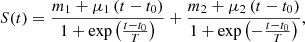 (A.1)
(A.1)
where m1, μ1, m2, μ2 are parameters of the linear functions, t0 is a turnover point at which S(t0) = 1/2(m1 + m2), and T is the characteristic timescale of the transition. We then fit this model to the HtS and StH transitions using the data from the H filter light curve. The reason we chose the H filter is that the nonthermal component contributes more to this filter, making it easier to determine the turnover points.
As a result, the transition boundaries can be universally expressed in terms of t0 and T. We define HtS start date as t0 − 2T and end date as t0 + 3T. Similarly, for the StH transition the start date is t0 − 3T and the end date is t0 + 2T. The choice of the offset factors is influenced by the slopes of the trends before and after the transition. For example, at t = t0 − 3T the contributions of the first and second trends are 5 and 95%, respectively, while at t = t0 − 2T the trends contribute 12 and 88%, respectively. As a result of such choice, the duration of the StH or HtS transitions is 5T and can be directly obtained from the fitted model parameters. An example of such outburst separation is shown in Fig. A.1a.
 |
Fig. A.1. Example of the phase separation during (a) rise and (b) decay of the 2010–2011 outburst. Colors and symbols are the same as in Fig. 4. The solid black line and dotted blue line (panel b) show the fitted models given by Eq. (A.1). Vertical dashed lines correspond to the boundaries between different phases. |
The boundaries between the decaying phase and the quiescence were determined in a similar manner. Because of the differences in the quiescent state baseline fluxes between outbursts, there is no common lower limit that is applicable to all of the outbursts simultaneously, which can be used to determine the end of the decay. Therefore, we fit a similar model to the decaying phase and quiescence data, for which we fix the parameter T at  d, corresponding to the very rapid change of the fitted model from one trend to another. We then use the turnover point t0 as a formal definition of the boundary between transition and quiescence (see Fig. A.1b, dotted blue line).
Our algorithm was also applied to the failed outbursts. We fit our model to the 2006 and 2009 events and adopted t0 − 2T and t0 + 2T as the transition boundaries. For the 2008 failed outburst, we used the turnover points t0 to subdivide the light curve into four parts. During this event GX 339-4 showed extremely erratic behavior with no clear manifestations of the nonthermal component, therefore the phase separation is rather arbitrary and is only required for comparison to other failed outbursts.
In order to compare the decaying phase of the failed and regular outbursts, we split the interval between the end of the SS and the beginning of the quiescence in half and mark the second half as DPh (see Fig. A.1b, pink open triangles). We also apply the algorithm to the rising phase of the 2002–2003 outburst, obtaining the starting date of the RPh.
Our algorithm is similar to that used by Buxton & Bailyn (2004) and is relatively insensitive to the data selection effects, as we eliminate the process of by-eye separation of data into groups prior to fitting (Kalemci et al. 2013). As a result, this method can be used to study and compare transition dates of the outbursts observed in other LMXB transients.
All Tables
Start and end dates of the outbursts and start dates of each identified outburst phase (in MJD).
ONIR filter effective wavelengths λ, zero-point fluxes F0 (Buxton et al. 2012) and derived extinction.
All Figures
|
Fig. 1. Observed ONIR magnitudes and corrected for the interstellar extinction fluxes of GX 339-4 in four ONIR filters (V, I, J and H). Vertical dashed lines separate data into 7 intervals corresponding to each of the regular/failed outbursts. |
| In the text | |
|
Fig. 2. X-ray light curves of GX 339-4. (a) Swift/BAT count rate in the 15–150 keV band, (b) ASM B (3–5 keV) flux, (c) ASM A (1.5–3 keV) light curve, and (d) ASM B/A hardness ratio. Orange points correspond to the soft states selected using ONIR data from four outbursts. Errors are 1σ. |
| In the text | |
|
Fig. 3. Joint posterior distribution of the model parameters. Contours correspond to 0.68, 0.95, and 0.99 probabilities. |
| In the text | |
|
Fig. 4. Evolution of magnitudes and colors of GX 339-4 throughout the outburst. V and V − H are observed magnitudes and colors, FV is corrected for the interstellar extinction flux, and αVH is the intrinsic spectral slope, computed assuming AV = 3.58 mag (see Eq. (5)). The dashed pink contour corresponds to the RPh, the top right solid blue contour represents the RHS, the top solid green arrow indicates the HtS transition, dotted orange contour corresponds to the SS, the bottom solid green arrow represents the reverse StH transition, the bottom solid blue contour indicates the DHS, and the solid pink contour corresponds to the DPh. The solid orange line gives the model blackbody curve with log10Nbb = 4.09, see Eq. (1) and the filled blue diamonds along the curve correspond to the temperatures marked on the right. The quiescent state is denoted with letter Q in the lower part of the diagram. |
| In the text | |
|
Fig. 5. Panel a: V versus V − H CMD of the 2002–2003 outburst. The filled upward-facing pink triangles correspond to the RPh, the filled blue circles indicate the RHS, the filled downward-facing green triangles represent the HtS transition, the filled orange squares indicate the SS, the open upward-facing green triangles correspond to the StH transition, the open blue circles indicate the DHS, the open downward-facing pink triangles correspond to the DPh, and the black crosses indicate the Q. Contours are the same as in Fig. 4. The typical 1σ errors are shown in the bottom left corner: the top orange cross corresponds to the bright states and is comparable to the plot symbol size; the bottom black cross corresponds to the quiescent state data, where observational errors are substantial. Panel b: ONIR H (top) and V (bottom) light curves of the same outburst. Symbols are the same as in panel a. Errors are 1σ and error bars are comparable to the symbols size. The solid black line represents the model, fitted to the part of the SS data. The gray area around the line denotes 1σ errors and also includes the contribution from the intrinsic scatter. Panel c: ASM A X-ray light curve. |
| In the text | |
|
Fig. 6. Same as Fig. 5, but for the 2004–2005 outburst. Panel c: the BAT data are shown with open gray squares starting from the second half of the 2004–2005 outburst. Errors are 1σ. |
| In the text | |
 |
Fig. 7. Same as Fig. 6, but for the 2007 outburst. |
| In the text | |
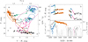 |
Fig. 8. Same as Fig. 6, but for the 2010–2011 outburst. |
| In the text | |
|
Fig. 9. Same as Fig. 6, but for the 2006 failed outburst. Blue circles indicate the bright phase of the outburst and black crosses indicate the quiescent state. The transition is shown with pink triangles. |
| In the text | |
|
Fig. 10. Same as Fig. 9, but for the 2008 failed outburst. Filled green triangles indicate the transition from the initial bright phase to the faint phase and open green triangles show the rebrightening. |
| In the text | |
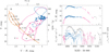 |
Fig. 11. Same as Fig. 9, but for the 2009 failed outburst. |
| In the text | |
|
Fig. 12. Sample of spectra from the soft state (orange squares), transition (green triangles), and the hard-state spectra (blue circles). The open symbols represent the StH state transitions, while the filled symbols indicate the HtS state transitions. Top panels (a–f): total observed spectra of the decaying part of the 2002–2003 outburst, the rising and decaying parts of the 2004–2005 outburst, the 2007 outburst, and the rising and decaying parts of the 2010–2011 outburst, respectively. Bottom panels (a*–f*): corresponding spectra after subtraction of the thermal component. Fluxes are corrected for the interstellar extinction; errors are 1σ. |
| In the text | |
|
Fig. 13. Selected spectra of the rising (top panels) and decaying (bottom panels) stages of regular outbursts. The 1σ errors are comparable to the symbol size. The solid orange and dotted blue and green lines correspond to the blackbody (BB) component in the soft and hard states and transitions, respectively. The dashed blue and green lines correspond to the power-law spectra of the hot flow (HF). The solid lines give the sums of the corresponding blackbody and the hot flow components. In panel b the HtS spectrum is not plotted because there are no observations with simultaneous measurements in three or more ONIR filters. Instead, two RHS spectra are shown, separated by ∼150 d, to highlight the evolution of both nonthermal and disk components (see also Fig. 6). |
| In the text | |
|
Fig. 14. Broadband spectra of GX 339-4 using the radio ATCA, mid-IR WISE, and ONIR SMARTS data. The figure shows four distinct spectral shapes for the source. The orange squares show the soft-state data from MJD 55301.36, the filled green circles and open green diamonds indicate the quasi-simultaneous ONIR and mid-IR data on MJD 55266.35. The open blue downward-facing triangles and open pink upward facing triangles show the mid-IR spectra measured 1.7 h before and after the quasi-simultaneous observation, respectively. The black crosses indicate one of the closest available ATCA radio observations (MJD 55269.80) that is used to constrain the jet properties. The lines show different model components: the dot-dashed orange line indicates the blackbody component, the dashed pink line shows the hot flow component, the dotted lines correspond to the jet model with different cutoff frequencies, and the solid lines give the sum of the three (blackbody + hot flow + jet) components. The sum of the blackbody and hot flow components for MJD 55266.41 is not shown for convenience because it fully coincides with the hot flow curve in the mid-IR. The 1σ errors are comparable with the symbol size. The WISE fluxes are adjusted by the normalization factors inferred from the fit (see Table 6). |
| In the text | |
|
Fig. 15. Quasi-simultaneous ONIR νHFH vs. X-ray 1.5−12 keV flux diagram. The X-ray data are taken from all three ASM bands. The colors and symbols are the same as in Fig. 5 and errors are 1σ. 2002–2003 (panel a), 2004–2005 (b), 2007 (c), and 2010–2011 (d) outbursts. |
| In the text | |
|
Fig. 16. Schematic representation of the evolution of GX 339-4 spectra during the rising phase hard state and HtS transition of an outburst. The dotted pink line indicates the RPh hard spectrum, the solid blue line corresponds to the RHS, and the dashed green line represents the HtS transition. The vertical black arrows indicate the transition sequence. Characteristic turnover frequency of each spectrum and the V filter frequency are shown with the vertical dashed lines. Characteristic spectral slopes in the ONIR and X-ray ranges are shown with αONIR and αX. |
| In the text | |
|
Fig. A.1. Example of the phase separation during (a) rise and (b) decay of the 2010–2011 outburst. Colors and symbols are the same as in Fig. 4. The solid black line and dotted blue line (panel b) show the fitted models given by Eq. (A.1). Vertical dashed lines correspond to the boundaries between different phases. |
| In the text | |
Current usage metrics show cumulative count of Article Views (full-text article views including HTML views, PDF and ePub downloads, according to the available data) and Abstracts Views on Vision4Press platform.
Data correspond to usage on the plateform after 2015. The current usage metrics is available 48-96 hours after online publication and is updated daily on week days.
Initial download of the metrics may take a while.