| Issue |
A&A
Volume 690, October 2024
|
|
|---|---|---|
| Article Number | A6 | |
| Number of page(s) | 13 | |
| Section | Stellar structure and evolution | |
| DOI | https://doi.org/10.1051/0004-6361/202450337 | |
| Published online | 25 September 2024 | |
The role of outflows in black-hole X-ray binaries
1
University of Crete, Physics Department & Institute of Theoretical and Computational Physics, 70013 Heraklion, Crete, Greece
2
Institute of Astrophysics, Foundation for Research and Technology-Hellas, 71110 Heraklion, Crete, Greece
Received:
12
April
2024
Accepted:
5
July
2024
Abstract
Context. The hot inner flow in black-hole X-ray binaries is not just a static corona rotating around the black hole: it must be partially outflowing. It is therefore a mildly relativistic “outflowing corona”. We have developed a model in which Comptonization takes place in this outflowing corona. In all of our previous work, we assumed a rather high outflow speed of 0.8c.
Aims. Here, we investigate whether an outflow with a significantly lower speed can also reproduce the observations. Thus, in this work we consider an outflow speed of 0.1c or less.
Methods. As in all of our previous work, we used a Monte Carlo code to compute not only the emergent X-ray spectra, but also the time lags that are introduced to the higher-energy photons with respect to the lower-energy ones via multiple scatterings. We also record the angle (with respect to the symmetry axis of the outflow) and the height at which photons escape.
Results. Our results are very similar to those of our previous work, with some small quantitative differences that can be easily explained. We are again able to quantitatively reproduce five observed correlations: (a) the time lag as a function of Fourier frequency, (b) the time lag as a function of photon energy, (c) the time lag as a function of Γ, (d) the time lag as a function of the cutoff energy in the spectrum, and (e) the long-standing radio–X-ray correlation – and all of them with only two parameters, which vary in the same ranges for all the correlations.
Conclusions. Our model does not require a compact, narrow relativistic jet, although its presence does not affect the results. The essential ingredient of our model is the parabolic shape of the Comptonizing corona. The outflow speed plays a minor role. Furthermore, the bottom of the outflow, in the hard state, looks like a “slab” to the incoming soft photons from the disk, and this can explain the observed X-ray polarization, which is along the outflow. In the hard-intermediate state, we predict that the polarization of GX 339−4 will be perpendicular to the outflow.
Key words: binaries: general / stars: black holes / stars: winds / outflows
Corresponding authors; This email address is being protected from spambots. You need JavaScript enabled to view it. , This email address is being protected from spambots. You need JavaScript enabled to view it. .
© The Authors 2024
 Open Access article, published by EDP Sciences, under the terms of the Creative Commons Attribution License (https://creativecommons.org/licenses/by/4.0), which permits unrestricted use, distribution, and reproduction in any medium, provided the original work is properly cited.
This article is published in open access under the Subscribe to Open model. This email address is being protected from spambots. You need JavaScript enabled to view it. to support open access publication.
1. Introduction
It is typically accepted that black-hole X-ray binaries (BHXRBs) broadly consist of an accretion flow (a geometrically thin, cool outer disk and a geometrically thick, hot inner flow) and a narrow relativistic jet. The jet emits in the radio and the infrared, and the hot inner flow acts as a corona that up-scatters soft disk photons to produce the hard X-rays.
The energy spectrum is nicely explained in the above picture as follows: (a) the radio and at least part of the infrared come from the jet, (b) the optical, ultraviolet, and some soft X-rays come from the accretion disk, and (c) hard X-rays come from the corona (for a review, see Remillard & McClintock 2006). On the other hand, it is well known that the spectra of BHXRBs are almost infinitely degenerate, in the sense that if one is granted freedom on the geometry of the source, the selection between thermal and nonthermal electrons, their energy distribution, and the optical depth to electron scattering, almost any observed energy spectrum can be fitted.
For energies above ∼2 keV, the harder photons are observed to lag with respect to softer ones. These lags have been explained as the result of propagating fluctuations in the hot inner flow (Nowak et al. 1999a; Kotov et al. 2001; Arévalo & Uttley 2006; Uttley et al. 2011; Uttley & Malzac 2023), light-travel times in the outflow (Reig et al. 2003), or impulsive bremsstrahlung injection occurring near the outer edge of the corona (Kroon & Becker 2016), or as the evolution timescales of magnetic flares produced when magnetic loops inflate and detach from the accretion disk (Poutanen & Fabian 1999). However, the observed correlation of the lags with the photon-number power-law index, Γ, of the hard X-rays (Kylafis & Reig 2018; Reig et al. 2018) and with the high-energy cutoff, Ec (Altamirano & Méndez 2015) suggests a common origin for the hard X-rays and the time lags. Likewise, the fact that the time lag–Γ correlation is inclination-dependent (Reig & Kylafis 2019) is also difficult to explain with the propagating-fluctuations model.
An important fact that has been neglected in the above picture is that the Bernoulli integral of the hot inner flow is positive (Blandford & Begelman 1999). This means that the matter cannot fall into the black hole. Thus, part of the hot inner flow must escape as an outflow to leave the rest with a negative Bernoulli integral. In other words, the hot inner flow is not just a static corona rotating around the black hole, but a wind-like “outflowing corona”.
We have been promoting the idea that the above outflow from the hot inner flow is the place where the X-ray spectrum is shaped. The reason is the following: The outflow lies above and below the hot inner flow. Thus, soft photons that are up-scattered in the hot inner flow must, before they escape, traverse the outflow, where they continue the scattering process. Since after a few scatterings the photons “forget” their initial energy, it is the scattering in the outflow that determines the emergent X-ray spectrum.
This picture has the advantage that it is very simple. All it requires is a parabolic outflow in which Compton up-scattering of soft photons from the accretion disk takes place. No additional mechanism is required for the time lags. They come naturally with the Compton up-scattering. The harder photons are scattered more times than the softer ones, spend more time in the outflow, and therefore come out later than the softer ones. The size of the outflow and its optical depth determine the magnitude of the time lags. Also, the fact that the time lags and the hard X-ray spectrum are produced by the same process (Comptonization) means that it is not surprising that the two are correlated (Reig & Kylafis 2015; Kylafis & Reig 2018). Furthermore, the Comptonized X-ray spectra that come out of the outflow are anisotropic because of the shape of the outflow (parabolic) and the outflow speed (v0 = 0.8c). The harder photons come out mainly along the outflow (large optical depth) and the softer ones mainly perpendicular to it (smaller optical depth). This, then, naturally explains the inclination dependence of the time lag–Γ correlation (Reig & Kylafis 2019).
The parabolic outflow also emits radio waves. In fact, the whole spectrum from the radio to hard X-rays can be explained in the outflow model (Markoff et al. 2001; Giannios 2005). In addition, since the same electrons do both the Compton up-scattering and the radio emission via the synchrotron mechanism, it is not surprising that the radio flux correlates with the X-ray flux (Corbel et al. 2013; Kylafis et al. 2023).
In our previous works, we used the word “jet” to refer to the outflow (i.e., anything outflowing was called a jet). This name now appears inappropriate. Our work reveals that a narrow relativistic jet is not required in this picture. There is no problem if it exists, but it is not necessary.
Here, we want to distinguish between the jet in BHXRBs, which is narrow (a few Rg at its base, where Rg is the gravitational radius) and relativistic (v0 ≳ 0.7c), and the outflow in BHXRBs, which is wind-like, broad (10 − 103 Rg at its base), and nonrelativistic. The outflow speed cannot be lower than the local escape speed, which is  , with R the radial distance. This means that the outflow speed, v0(R), is > 0.45c at R = 10 Rg and > 0.045c at R = 103 Rg. Since in our previous work we used v0 = 0.8c, which for a wide outflow (say 102 − 103 Rg) implies a huge mass-outflow rate unless the matter consists of electron–positron pairs (not likely in BHXRBs), we need to demonstrate that an outflow with a significantly lower speed reproduces the above correlations. This is what we demonstrate in the present paper, but with v(R) constant (set to 0.1c = v0) and not a function of R. The reason for this is because we do not know the mass-outflow rate at every radius, R, which we would need to compute the density in the outflow at a given height as a function of radius. Thus, we feel that a demonstrative calculation, with a low constant outflow speed, will suffice. We discuss this in Sects. 2.7 and 3.
A detailed description of our model is given in Appendix A, where we also describe how our Monte Carlo code works. In Sect. 2 we discuss our results, and in Sect. 3 we give a summary and present our conclusions.
2. Results
In the following sections we present the observational results that our model is capable of reproducing. These results are to be compared with those published over the years in Reig et al. (2003, 2018), Kylafis et al. (2008, 2020), Reig & Kylafis (2015, 2019, 2021), and Kylafis & Reig (2018). Our goal is to demonstrate that a nonrelativistic, wind-like outflow (i.e., v0 = 0.1c) can reproduce our previous results (where a mildly relativistic outflow with v0 = 0.8c was used), which in turn, explain many observations and correlations. In this work, we have assumed that the observer sees the system at an intermediate inclination angle. Hence, we combined all the escaping photons with directional cosines in the range 0.2 ≤ cos θ ≤ 0.6. A full description of the meaning of the model parameters is given in Appendix A.
2.1. Energy spectra
The observed X-ray spectral continuum (0.1−200 keV) of BHXRBs consists of a soft thermal component and a hard nonthermal component. The thermal component is modeled as a multi-temperature blackbody and dominates the spectrum below ∼2 keV (Mitsuda et al. 1984; Merloni et al. 2000). Its origin is attributed to a geometrically thin, optically thick accretion disk (Shakura & Sunyaev 1973). The nonthermal component is well described by a power law with a high-energy exponential cutoff. This component is believed to be the result of Comptonization of low-energy photons from the accretion disk (Sunyaev & Truemper 1979), by energetic electrons in a configuration that is still under debate.
During X-ray outbursts, BHXRBs go through different spectral states (McClintock & Remillard 2006; Belloni 2010), of which the two main ones are the soft and hard states (Done et al. 2007). Intermediate states – the hard-intermediate state (HIMS) and the soft-intermediate state – occur when the source transits from these basic states. Each state is characterized by a different contribution of the thermal and power-law components. In the soft state, the thermal blackbody component dominates the energy spectrum, with no or very weak power-law emission (Remillard & McClintock 2006; Dexter & Quataert 2012). In this state the radio emission is quenched. In the hard state (HS), the soft component is weak or absent, whereas the power law extends to a hundred keV or more with photon-number index Γ in the range 1.2 − 2. In the HIMS, the power-law component is still present, albeit with a steeper slope (i.e., a larger Γ) than in the HS, while the blackbody component starts to appear (McClintock & Remillard 2006; Castro et al. 2014), if it was not already there in the HS. In the HS and the HIMS, the systems shine bright in the radio band.
In our model, the Comptonizing medium is the outflow, which extends laterally to relatively large distance (a few hundred Rg at its base) from the black hole. Therefore, our model is relevant for the HS and HIMS and it should be able to reproduce a power law with photon index in the range 1.2 − 2.6, as measured in the observations.
The main parameter that affects the slope of the continuum is the optical depth, τ∥ (τ⊥ is uniquely determined given τ∥ and R0), as it is directly related to the number of scatterings in the outflow. We can reproduce the observed range of the photon index, Γ, in the HS and the HIMS by changing the optical depth, τ∥. Figure 1 shows the resulting energy spectra of our model. Each spectrum corresponds to a model with R0 = 400 Rg, Lorentz γ0 = 1.14, and variable τ∥ between 1 and 4.5, while the rest of the parameters are kept fixed at the reference values given in Table A.1. The spectra have been normalized by the flux at 1 keV. The nonrelativistic outflow (v0 = 0.1c) requires lower values of the optical depth to reproduce the photon index of the HS and HIMS, compared to the mildly relativistic outflow that we used before (v0 = 0.8c), for which τ∥ ranged between 2 and 11 (Reig et al. 2003; Kylafis & Reig 2018).
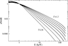 |
Fig. 1. Energy spectra for different optical depths (from top to bottom): τ∥ = 4.5, 4, 3.5, 3, 2.5, 2, 1.5, and 1. The width at the base of the outflow was R0 = 400 Rg and the Lorentz factor of the coasting electrons was γ0 = 1.14. The spectra have been normalized by the flux at 1 keV. |
2.2. Lag–frequency correlation
When two light curves obtained at two separate energy bands (say, a hard and a soft) are cross-correlated, lags are observed between the hard and soft bands. Positive or hard lags mean that the hard photons lag the soft photons. This is always the case at energies above ∼2 keV, that is, at energies where the power-law component, typically associated with Comptonization, dominates. The magnitude of this lag strongly depends on Fourier frequency and on the energy bands considered (Miyamoto et al. 1988; Vaughan & Nowak 1997; Cui et al. 1997; Poutanen 2001; Pottschmidt et al. 2003), but typically it is in the range of 1−100 ms. A different type of lags are the so-called reverberation or soft lags, where the soft photons (say, around 0.5 keV) lag the hard ones. These can result from the delay between the hard photons that hit the accretion disk, are absorbed there, and are emitted as soft photons, and the hard photons that reach the observer directly, before the soft photons (Uttley et al. 2014). In this case the soft band is defined at energies below ∼1 keV, as it comes from the disk (Uttley et al. 2011). Reverberation lags are typically negative, that is, soft photons lag hard photons (Kara et al. 2019). This is explained by the extra path that the absorbed hard X-rays have to travel. In this work we deal with positive lags only.
The positive lags, calculated at energies above ∼2 keV, can naturally be attributed to inverse Comptonization. In order to acquire their energy, harder photons scatter more times than less hard photons, and hence they stay longer in the Comptonizing medium before they escape. In this context, time lags simply signify the difference in light-travel time of photons within the Comptonizing region. A different explanation of the time lags was offered by Lyubarskii (1997, see also Kotov et al. 2001; Arévalo & Uttley 2006). In this model, the lags result from viscous propagation of mass-accretion fluctuations within the inner regions of the accretion flow.
Observations of time lags in the HS show that they roughly follow a power-law dependence on Fourier frequency of the form tlag ∝ ν−0.8 ± 0.1 (Crary et al. 1998; Nowak et al. 1999b; Cassatella et al. 2012). Our model reproduces quantitatively this nearly 1/ν dependence of the time lags on Fourier frequency, and this is shown in Fig. 2. The time of flight of all escaping photons was recorded in Nbins = 8192 time bins of duration 1/64 s each. This time was computed by adding up the path lengths traveled by each photon and dividing by the speed of light. Then, we considered the light curves of two energy bands: soft or reference band (2−6 keV) and hard (6−15 keV). We identified the phase lag, ϕ, between the signals of the two bands as the phase of the complex cross-vector, and from it the corresponding time lag τ = ϕ/2πν as a function of Fourier frequency ν.
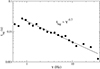 |
Fig. 2. Time lag as a function of Fourier frequency. The model shown corresponds to τ∥ = 3, R0 = 400 Rg, and γ0 = 1.14. |
The black filled circles in Fig. 2 correspond to a model with τ∥ = 3, R0 = 400 Rg, and γ0 = 1.14. The values of these parameters are not crucial, as long as τ∥ is not too large. The case of large τ∥ will be explored in a subsequent paper (Reig et al., in preparation). It is straightforward to explain qualitatively the above approximately 1/ν dependence of the time lags, because Compton scattering acts like a filter that cuts off the high frequencies. We explain this below.
For the sake of this argument, we can think of the outflow as a series of spheres with radii R1 < R2 < R3 < …, one on top of the other, with the smaller one at the bottom (see Fig. 3). This is a discrete visualization of the parabolic outflow with radius R(z) = R0(z/z0)1/2, where z0 is the height above the black hole at which the outflow starts. If τ∥ is of order unity, then soft photons from the accretion disk, that enter the outflow from below, can scatter in any of the above spheres. The source of soft input photons is indicated in Fig. 3 by a star. Consider soft photons that have an intrinsic variability with period P (i.e., frequency ν = 1/P) and scatter in one of the spheres. If they scatter in the sphere with radius R1, this variability will be significantly reduced if the time delay due to Compton scattering, t1 = R1/c, is comparable to or larger than P. This means that all frequencies larger than 1/t1 = c/R1 will be essentially washed out. If the scattering occurs in the sphere with radius R2, with typical time delay t2 = R2/c, then all frequencies larger than 1/t2 = c/R2 will be washed out, and so on. In other words, if the time delay due to Compton scattering is t, then all frequencies of variability in the input photons larger than 1/t will be washed out. The Monte Carlo Comptonization in a parabolic outflow reproduces the ν−α dependence, with α = 0.7 − 0.9. If the outflow is not parabolic, then Comptonization does not reproduce this frequency dependence. Such outflows will be examined in a subsequent paper, and they seem to be related with the outlier sources, that is to say, the sources that do not obey the regular radio–X-ray correlation (Gallo et al. 2003; Corbel et al. 2003; Kylafis et al. 2023).
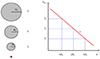 |
Fig. 3. Explanation of the frequency dependence of the time lags. |
2.3. Lag–energy correlation
In the previous section, we showed that the hard lags observed in the HS of BHXRBs can be due to the fact that the harder photons have undergone more scatterings inside the outflow (the region where the energetic electrons reside) than lower-energy photons. Also, the energy of the photons changes with every scattering, with an increase in energy, on average. Therefore, both the final amplitude of the lags and the energy with which the photons escape depend on the number of scatterings. Comptonization models predict a log-linear energy dependence in the lags, approximately what is observed (Nowak et al. 1999b; Kotov et al. 2001; Stevens & Uttley 2016). The slope of the relation depends on the range of Fourier frequencies considered to compute the average lag, becoming flatter as the frequency increases (Kotov et al. 2001; Uttley et al. 2011). Observations with good signal-to-noise show that the relation may be more complex than a simple log-linear law, with some bumps or breaks, around the energy of the iron line at 6.4 keV (Kotov et al. 2001; Stevens & Uttley 2016).
Figure 4 shows the energy dependence of the time lag, as computed from our model with R0 = 180 Rg, τ∥ = 2, and γ0 = 1.14. The data are from Kotov et al. (2001) for Cyg X–1. The reference band is 2.7−4 keV and the frequency range of the lag calculation is 0.05−5 Hz, to approximately match the values used by Kotov et al. (2001). In general terms, our model reproduces the approximately linear relation between tlag and log E quite well.
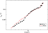 |
Fig. 4. Lag as a function of energy. Black filled circles represent the observations for Cyg X–1. The model shown as red empty circles corresponds to τ∥ = 2, R0 = 180 Rg, and γ0 = 1.14. |
2.4. Lag–Γ correlation
Numerous studies have shown that the spectral (e.g., photon index, Γ, and cutoff energy, Ec) and timing (characteristic frequency of the broadband noise and quasi-periodic oscillations, time lags, or phase lags) quantities in BHXRBs display tight correlations (Di Matteo & Psaltis 1999; Pottschmidt et al. 2003; Kalemci et al. 2003, 2005; Shaposhnikov & Titarchuk 2009; Stiele et al. 2013; Shidatsu et al. 2014; Grinberg et al. 2014; Kalamkar et al. 2015; Altamirano & Méndez 2015; Kylafis & Reig 2018; Reig et al. 2018; Reig & Kylafis 2019; Karpouzas et al. 2021; Méndez et al. 2022). These correlations represent convincing evidence that the timing and spectral properties of the sources are closely linked.
We have demonstrated that our outflow model is able to reproduce the observed correlation between time lag and Γ, not just for a specific source Cyg X–1 (Kylafis et al. 2008) or GX 339–4 (Kylafis & Reig 2018), but in general for BHXRBs as a group (Reig et al. 2018). All these correlations were reproduced varying only the optical depth τ∥ and the width at the base of the outflow R0. In those models, the Lorentz factor was γ0 = 2.24, which resulted from a high outflow speed v0 = 0.8c and a moderate perpendicular component v⊥ = 0.4c. In this work, we show that the outflow speed is not a critical parameter of the model and that a nonrelativistic outflow with v0 = 0.1c can also reproduce the observations. We take v⊥ = 0.47c, so that γ0 = 1.14.
In Fig. 5 we show the tlag–Γ correlation for Cyg X–1 (left panel) and for GX 339–4 (right panel). The black empty circles represent the observations and the blue filled circles our models. These figures are to be compared with Fig. 2 in Kylafis et al. (2008) and Fig. 2 in Kylafis & Reig (2018). The energy and frequency ranges used to compute the lags are the same as in the above references, namely between the bands 2 − 4 keV and 8 − 14 keV in the frequency range 3.2 − 10 Hz for Cyg X–1, and between 2 − 6 keV and 9 − 15 keV in the 0.05 − 5 Hz range for GX 339–4. This comparison reveals that even if the outflow speed is reduced from 0.8c to 0.1c, the range of variability of the optical depth τ∥ and radius R0 does not change significantly. At the lower outflow speed (v0 = 0.1c), the fits require a slightly smaller optical depth and a larger radius, 1 ≲ τ∥ ≲ 6 and 50 Rg ≲ R0 < 1500 Rg compared to 2 ≲ τ∥ ≲ 11 and 30 Rg ≲ R0 ≲ 600 Rg for the v0 = 0.8c case.
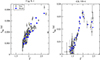 |
Fig. 5. Correlation between time lag and photon index, Γ, for Cyg X–1 (left) and GX 339–4 (right). The data for Cyg X–1 come from Pottschmidt et al. (2003, see also Kylafis et al. 2008) and for GX 339–4 from Kylafis & Reig (2018). Black empty circles represent the observations, and the filled blue circles correspond to the models, which are produced with γ0 = 1.14 and the values of τ∥ and R0 that are shown in Fig. 6. |
2.5. τ∥–R0 correlation
One remarkable outcome of our model is the correlation that we have found between the optical depth τ∥ and the radius R0 at the base of the outflow (Kylafis et al. 2008; Kylafis & Reig 2018; Reig et al. 2018; Reig & Kylafis 2019). As we mentioned before, we can reproduce a number of observations and correlations by changing only the two basic parameters τ∥ and R0. Surprisingly, these two parameters do not vary independently of one another, but in a correlated manner, following a power law τ∥ ∝ R0−β, in the HS of BHXRBs. Thus, for the modeling of the HS of BHXRBs we basically need one parameter, not two. Figure 6 shows this correlation. The points correspond to the models that were used for the explanation of the tlag–Γ correlations shown in Fig. 5. The correlations break down when the source enters the HIMS. The index β is not unique for all BHXRBs, but different sources display different values of β. For example, for Cyg X–1, β = 0.69 and for GX 339–4, β = 0.38. This is to be expected since the amplitudes of the lags of the two sources are significantly different.
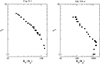 |
Fig. 6. Correlation between the optical depth, τ∥, and the radius of the outflow at its base, R0, for Cyg X–1 (left) and GX 339–4 (right). The values of the parameters R0 and τ∥ are those that were used in the models that produced Fig. 5. |
2.6. Lag–cutoff energy correlation
Another interesting result observed in the BHXRB GX 339–4 is the correlated evolution of the cutoff energy, Ec (in its energy spectrum) and the phase lag, ϕlag, of harder photons compared to less hard ones, as the source progresses along the HS (Motta et al. 2009; Altamirano & Méndez 2015). As the X-ray flux increases, the cutoff energy decreases and the amplitude of the time lag increases (see Fig. 7 in Altamirano & Méndez 2015). We show in Sect. 2.1 that higher optical depths τ∥ result in harder spectra (the photons are scattered more and gain more energy from the energetic electrons of the outflow). Likewise, by increasing R0, the spectrum also hardens, because larger R0 translates to larger Thomson optical depth τ⊥ perpendicular to the axis of the outflow and therefore more scatterings of the photons. For the same reason, the amplitude of the lags increases when the optical depth and/or the radius of the outflow increase. The cutoff energy, Ec, has a weak dependence on τ∥ and R0, but a rather strong dependence on v⊥. This is because the cutoff is mainly determined by the energetics of the electrons and v⊥ determines the maximum energy gain of the soft photons (Giannios et al. 2004; Giannios 2005).
In Reig & Kylafis (2015), we reproduced the correlation between the cutoff energy, Ec, and the phase lag, ϕlag, observed in the BHXRB GX 339–4 by changing τ∥, or v⊥, or both in a correlated way. In that work, we kept R0 fixed at 100 Rg. However, as the outburst progresses (i.e., as the X-ray flux increases), we expect that both τ∥ and R0 will vary, as we have already shown in Sect. 2.4. Our model requires that as the source moves from the HS to the HIMS, τ∥ decreases and the R0 increases.
Here we reproduce again the correlation between lag and cutoff energy in a slightly different form (Fig. 7). We used the time lag instead of the phase lag and the results of our own analysis instead of data from Motta et al. (2009) and Altamirano & Méndez (2015). The details of the analysis can be found in Reig et al. (2018). We used data from the 2006 outburst of GX 339–4. In Fig. 7, black filled circles represent the observations and blue filled circles the results of our models. We emphasize that the models displayed in Fig. 7 are the same models (i.e., the same combinations of τ∥ and R0) that reproduced the tlag–Γ correlation of Fig. 5, simply adjusting slightly the v⊥. The values of v⊥ that reproduce the observations vary in the range 0.41c − 0.46c.
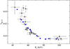 |
Fig. 7. Relationship between the time lag and cutoff energy. Black circles represent the observations for the BHXRB GX 339–4. The blue circles correspond to our models. The values of the parameters R0 and τ∥ are the same as in the models that were used in Fig. 5. |
2.7. Inclination effects
In Reig et al. (2018), we investigated the correlation between tlag and Γ for a large number of BHXRBs. The data in the correlation showed a large scatter that was explained as an inclination effect (Reig & Kylafis 2019). Systems seen at low inclination exhibit a stronger correlation. In high-inclination systems, the correlation is rather weak. We also showed that low- and intermediate-inclination systems tend to have harder spectra (see also Reig et al. 2003) and a larger amplitude of time lags. The explanation is that, in a mildly relativistic outflow, the high bulk speed of the electrons provides a boost on the photons that makes them scatter preferentially in the forward direction. These photons travel longer distances and suffer more scatterings than photons that escape perpendicularly to the outflow axis. Therefore, photons that escape at small to moderate angles, θ, with respect to the outflow axis lead to harder spectra (lower photon index) because they undergo more scatterings and longer lags because they travel longer distances.
Figure 8 shows the dependence of the photon index on the escaping angle for the case of a mildly relativistic outflow with v0 = 0.8c (blue dots) and a nonrelativistic outflow with v0 = 0.1c (black dots). Here θ is the angle between the observer and the outflow axis (i.e., photons with cos θ ∼ 1 escape along the axis, while cos θ ∼ 0 escape perpendicular to the outflow axis). The parameters of the models shown are τ∥ = 5.5 and R0 = 140 Rg for the mildly relativistic outflow and τ∥ = 3.5 and R0 = 150 Rg for the nonrelativistic outflow.
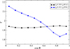 |
Fig. 8. Photon index as a function of escaping direction. The blue dots are for v0 = 0.8c and the black dots for v0 = 0.1c. In the inset, we show the corresponding Lorentz factor, γ0. |
As we indicated in the Introduction, our model with constant v0 = 0.1c is only demonstrative because in reality the escape speed is not expected to be constant, but a function of R, and it ranges from 0.58c at R = 6 Rg to 0.045c at R = 103 Rg. Thus, the real outflow has a central fast part and a progressively slower outer part. Without this variable v0(R) it is not possible to compute accurately the spectra as a function of inclination.
2.8. Disk illumination
In our model, soft photons are injected isotropically upward at the base of the outflow. Depending on τ∥ and the initial direction, photons may escape un-scattered or after a number of scatterings. After escape, we record their energy, angle of escape (with respect to the outflow axis), height from the black hole, and travel time in the outflow. Hence, the code also computes the back-scattered photons (i.e., photons with escaping angle θ > π/2). Some of these photons will be absorbed by the accretion disk and others will be reflected by it. The code, in its current version, does not account for reflection, but we can measure the number of photons that hit the accretion disk. In other words, we can compute the irradiation spectrum.
In Reig & Kylafis (2021), we showed that the fraction of back-scattered photons increases as the Lorentz factor γ0 decreases. The reason is that in nonrelativistic outflows the scattering is nearly isotropic, whereas when the outflow velocity is high, there is a strong forward boost, as explained in the previous section. Although in our model photons can interact with electrons anywhere in the outflow, most of the scatterings occur close to the black hole, not far away from the base of the outflow if the outflow velocity is low.
Figure 9 compares the energy distribution of the photons that illuminate the disk – that is, the “disk” spectrum (solid line) – with the “direct” spectrum of the photons from the outflow, seen by observers for typical LS and HIMS spectra. Unlike the relativistic case with v0 = 0.8c, where the disk spectrum was much softer than the direct one (see Fig. 3 of Reig & Kylafis 2021), here the disk and the direct spectra are very similar. The spectra, both direct and disk, are slightly softer in the HIMS than in the HS, in agreement with observations.
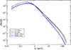 |
Fig. 9. Comparison of the “direct” and “disk” spectra. The direct spectrum is the spectrum seen by observers at infinity at an inclination θ ∼ 40°, and the disk spectrum is the spectrum of the photons that are back-scattered and illuminate the disk. The parameters of the models used in this figure for the LS are τ∥ = 2.5, R0 = 500 Rg, and γ0 = 1.14 and for the HIMS τ∥ = 1.5, R0 = 1400 Rg, and γ0 = 1.14. |
Another way to investigate the irradiation of the accretion disk by the primary source is by computing the emissivity profile, which is the radially dependent flux irradiating the disk by the source. For a standard Shakura-Sunyaev accretion disk, it is parameterized as a power law F(r)∝r−q, with q the emissivity index. The standard behavior is q = 3 (Dauser et al. 2013). To compute the emissivity index, we divided the accretion disk into radial zones and computed the number of photons per unit area that irradiate a given zone. For the sake of the computation and in order to compare with the lamppost geometry, we collapsed the outflow to R0 = 1 Rg. We find that for Rdisk ≳ 10 Rg, the radial dependence of the irradiated flux on the disk does follow a power law with q = 3, that is, the expected value for a standard Shakura-Sunyaev disk1.
Fig. 10 shows the distribution of distances h from the black hole from which the photons that hit the accretion disk escape. We show this distribution for different values of τ∥ (top panel) and R0 (bottom panel) and two Lorentz factors γ0 = 1.10 and γ0 = 2.24 (i.e., v0 = 0.1c and v0 = 0.8c, respectively). As expected, most of the photons escape within a few Rg, but a significant fraction of the photons that hit the accretion disk also escape at tens of to a few hundred Rg. This figure also confirms the fact that disk illumination increases as the outflow speed decreases. The vertical axis in Fig. 10 is reminiscent of the reflection fraction, defined as the number of emitted photons of the primary source that hit the accretion disk, NAD, over the number of photons escaping to infinity, N∞ (Dauser et al. 2014, 2016)2.
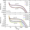 |
Fig. 10. Fraction of photons that hit the accretion disk over the total number of photons as a function of distance from the black hole at which they escape, h, for different values of the optical depth, τ∥, and radius, R0, of the outflow. The distribution is shown for a mildly relativistic outflow (γ0 = 2.24, i.e., v0 = 0.8c) and a nonrelativistic outflow (γ0 = 1.10, i.e., v0 = 0.1c). |
2.9. The radio–X-ray correlation
One of the most tight correlations in BHXRBs is the radio–X-ray correlation (Hannikainen et al. 1998; Corbel et al. 2000, 2003; Gallo et al. 2003; Bright et al. 2020; Shaw et al. 2021). The correlation extends over five orders of magnitude in radio flux and eight orders of magnitude in X-rays. The radio–X-ray correlation is in the form of a power law,  , where δ ≈ 0.5 − 0.7 (Gallo et al. 2012; Corbel et al. 2013). In addition to the main correlation, a group of outliers populate the FR − FX plane (Gallo et al. 2012). The group of outliers is associated with radio quiet sources, while most of the sources that follow the standard correlation are radio loud systems (Espinasse & Fender 2018). This difference in radio emission could be an inclination effect (Motta et al. 2018), though other possibilities should be examined. Here we show that our model can reproduce the standard FR − FX correlation. In particular, for the best-studied BHXRB GX 339–4, for which the correlation stands for more than five orders of magnitude in X-ray flux, the exponent is δ = 0.62 ± 0.01 (Corbel et al. 2013).
We followed the same procedure as in Kylafis et al. (2023), where we reproduced the FR–FX correlation for the case of a mildly relativistic outflow (i.e., v0 = 0.8c). From the X-ray observations of the 2007–2008 outburst of GX 339–4, we obtained a relationship between X-ray flux and photon-number spectral index Γ. We re-binned the data in bins of 0.05 in Γ for the HS and 0.1 for the HIMS. The error in the flux was computed as the standard deviation of the data in each bin. From our model, we computed the radio flux and the X-ray spectrum (i.e., the spectral index, Γ) for each set of input parameters (R0, τ∥). Thus, we obtained an entirely theoretical relationship between radio flux and photon index Γ. We stress that our model input parameters are not arbitrary, but they are exactly the same as those in Fig. 6 (right panel), which reproduce the correlation between time lag and Γ, shown in Fig. 5 (right panel). Thus, we attempt to explain two correlations with the same model parameters.
From the observed FX–Γ correlation and the computed FR–Γ one, we matched the radio and X-ray fluxes that have the same or very similar value of Γ, and plotted one against the other. The result is shown in Fig. 11. We refer the reader to Appendix A (see also Giannios 2005; Kylafis et al. 2023) for the computation of the radio flux with our model as well as the details of the analysis of the X-ray observations. The black line Fig. 11 is not a fit to the blue dots, but it is the observational correlation of (Corbel et al. 2013). The blue dots correspond to the HS and the red dots to the HIMS. The only quantity that we had to change in this calculation, as compared with the one reported in Kylafis et al. (2023), is the magnetic field B0 at the base of the outflow. Here, its value is 2.9 × 10⁴ G.
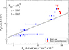 |
Fig. 11. Radio–X-ray flux correlation for GX 339–4. The models used to compute the radio flux and the theoretical Γ are the same as those that reproduce the time lag–Γ correlation displayed in Fig. 5. |
2.10. X-ray polarization
Recent results from the Imager X-ray Polarimetry Explorer (IXPE) mission (Weisskopf et al. 2022) have revealed that BHXRBs show polarization degrees in the X-ray band (2−8 keV) of a few percent and the polarization angle is aligned with the outflow (Krawczynski et al. 2022; Veledina et al. 2023; Ingram et al. 2023; Rodriguez Cavero et al. 2023). Since Comptonization in a slab (with Thomson optical depth in the plane of the slab much larger than in the perpendicular direction) gives rise to linear polarization perpendicular to the slab (Poutanen et al. 1996; Schnittman & Krolik 2010), people typically assume the Comptonizing corona to be in the form of a slab, perpendicular to the outflow, but without giving a physical justification for this. Also, models with a static Comptonizing region predict a lower polarization degree than the observed one. One way to produce higher polarization is by assuming that the inner disk is viewed at a higher inclination angle than the outer disk (Krawczynski et al. 2022). Another way is by considering an outflowing Comptonizing medium (Poutanen et al. 2023; Ratheesh et al. 2023).
Our model of a parabolic, outflowing corona naturally provides a Comptonizing, outflowing “slab” at its bottom. This is shown below, where, for simplicity of the expressions, we consider an instantaneous acceleration of the outflow to speed v0 at the bottom of it. For the full model with an acceleration region, the optical depths are calculated in Appendix A.
For a parabolic outflow, the radius of the outflow at height z is
 (1)
(1)
where R0 is the radius at the base of the outflow, which is at height z0. From the continuity equation
 (2)
(2)
where ne is the electron number density, mp is the proton mass, and Ṁ is the mass-outflow rate, one gets for the electron density
 (3)
(3)
where n0 is the density at z0. The Thomson optical depth τ∥(z) from z0 to z > z0 is
 (4)
(4)
while the perpendicular Thomson optical depth at height z is
 (5)
(5)
or
 (6)
(6)
The ratio of the optical depth τ∥(z) to the total optical depth along the outflow τ∥(H)≡τ∥ is
 (7)
(7)
which means that
 (8)
(8)
Here H is the height of the outflow that we take it to be H = 105 Rg, where Rg is the gravitational radius.
Figure 12 shows the variation of the parallel, τ∥, and the perpendicular, τ⊥, optical depths as functions of distance from the black hole, z, when an acceleration region is present (i.e., the physical case; see Appendix A) and when it is absent (i.e., the nonphysical, but simpler, case of instant acceleration). Figure 12 implies that, at its bottom, the outflow behaves like a slab, because τ⊥ ≫ τ∥. In Sect. 2.8 (see also Fig. 10) we indicated that most of the scatterings occur near the bottom of the accretion flow, especially in the HS, because the optical depth is high. Thus, in the HS, the bottom of the outflow is seen by the incoming soft photons as an “outflowing slab” and therefore the X-ray polarization is expected to be along the outflow. In the HIMS, on the other hand, the outflowing corona (at least for GX 339–4) is nearly transparent (τ∥ ∼ 1). The soft photons travel along the outflow and scatter on average once. Thus, in the HIMS, the X-ray polarization is expected to be perpendicular to the outflow.
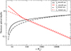 |
Fig. 12. Thomson optical depths (parallel and perpendicular to the outflow) as functions of distance from the black hole. We show two cases: instant acceleration of the outflow (dashed lines) and when an acceleration region is present, i.e., smooth acceleration (solid lines). We used a model with τ∥ = 5 and R0 = 100 Rg, where Rg is the gravitational radius. |
3. Summary and conclusion
We have demonstrated that we can reproduce most of the results from our previous works even with a nonrelativistic outflow. These are: (a) the energy spectrum (Fig. 1), (b) the dependence of the time lag on Fourier frequency (Fig. 2), (c) the log-linear dependence of the time lag on photon energy (Fig. 4), (d) the correlation between the time lag and the photon index, Γ, in GX 339–4 and Cyg X–1 (Fig. 5), (e) the time-lag–cutoff-energy correlation observed in GX 339–4 (Fig. 7), and (f) the fact that the outflow provides a natural lamppost for the hard X-ray photons that return to the disk (Fig. 10).
The reduction in the outflow speed implies that the fraction of back-scattered photons increases, and their spectrum displays about the same Γ as the photons directly escaping to the observer (unlike the models with v0 = 0.8c, which produce softer spectra for the photons that return to the disk compared to those that go directly to the observer). This is because the boost in the forward direction is highly reduced. Hence, the number of photons that travel greater distances decreases. Owing to the smaller boost along the outflow axis in the case of v0 = 0.1c, as compared to the case of v0 = 0.8c, the photon index is only slightly dependent on the inclination (Fig. 8), as expected. A more realistic calculation would require a parabolic outflow with a distribution of outflow velocities that decreases as one moves away from the axis. In other words, the outflow should be composed of a mildly relativistic and narrow part at its core and a less and less relativistic outflow at larger transverse distances.
As in the case of a mildly relativistic outflow (v0 = 0.8c), our model with v0 = 0.1c reproduces the observations by changing only two parameters: the optical depth along the outflow axis, τ∥, and the radius at its base, R0; since these two parameters are correlated (Fig. 6), our model actually has only one parameter. Our simulations in the present work (v0 = 0.1c and for GX 339–4) require a slightly smaller range in optical depth (1 ≲ τ∥ ≲ 6) and a slightly larger range in outflow radius (50 ≲ R0/Rg ≲ 1500) compared to the v0 = 0.8c case for which 2 ≲ τ∥ ≲ 11 and 30 ≲ R0/Rg ≲ 600. The mass-outflow rate is on the order of 1 − 5 times the Eddington rate for a 10 solar-mass black hole in the HS and 10 − 50 times the Eddington rate in the HIMS. We remark, however, that the simplifying assumption of a constant outflow speed makes the numbers unreliable. Future calculations, with a realistic outflow speed as a function of radius, will address this issue.
Finally, we note that in the HS (no matter what the outflow speed is), the bottom of the outflow, where most of the scatterings occur, is like a slab, which produces X-ray polarization parallel to the outflow. In the HIMS and for GX 339–4, for which τ∥ is of order unity, we predict that the polarization will be perpendicular to the outflow.
When relativistic effects are taken into account, steeper profiles are found in the inner parts of the accretion disk (Dauser et al. 2022) and a broken power law is used instead (Bambi et al. 2020). We note that because our model deals with broad outflows, relativistic effects are not expected to play any significant role in our results.
Here we have employed NAD/Nphot, instead of NAD/N∞, where Nphot is the total number of photons coming out from the outflowing corona and N∞ = Nphot − NAD.
Typically, Nbin = 8192, δt = 1/64 s. The energy bands are taken to match the data results that we want to reproduce. The same applies to the frequency range in which the average lags are computed.
Acknowledgments
We thank Alexandros Tsouros for offering us his code, which computes the radio emission from the outflow. We also thank an anonymous referee for a thorough reading of the manuscript, which resulted in useful comments.
References
- Altamirano, D., & Méndez, M. 2015, MNRAS, 449, 4027 [NASA ADS] [CrossRef] [Google Scholar]
- Arévalo, P., & Uttley, P. 2006, MNRAS, 367, 801 [Google Scholar]
- Asada, K., & Nakamura, M. 2012, ApJ, 745, L28 [NASA ADS] [CrossRef] [Google Scholar]
- Bambi, C., Brenneman, L. W., Dauser, T., et al. 2020, ArXiv e-prints [arXiv:2011.04792] [Google Scholar]
- Belloni, T. M. 2010, Lect. Notes Phys., 794, 53 [NASA ADS] [CrossRef] [Google Scholar]
- Blandford, R. D., & Begelman, M. C. 1999, MNRAS, 303, L1 [NASA ADS] [CrossRef] [Google Scholar]
- Bright, J. S., Fender, R. P., Motta, S. E., et al. 2020, Nat. Astron., 4, 697 [NASA ADS] [CrossRef] [Google Scholar]
- Cassatella, P., Uttley, P., Wilms, J., & Poutanen, J. 2012, MNRAS, 422, 2407 [NASA ADS] [CrossRef] [Google Scholar]
- Castro, M., D’Amico, F., Braga, J., et al. 2014, A&A, 569, A82 [NASA ADS] [CrossRef] [EDP Sciences] [Google Scholar]
- Corbel, S., Fender, R. P., Tzioumis, A. K., et al. 2000, A&A, 359, 251 [NASA ADS] [Google Scholar]
- Corbel, S., Nowak, M. A., Fender, R. P., Tzioumis, A. K., & Markoff, S. 2003, A&A, 400, 1007 [NASA ADS] [CrossRef] [EDP Sciences] [Google Scholar]
- Corbel, S., Aussel, H., Broderick, J. W., et al. 2013, MNRAS, 431, L107 [NASA ADS] [CrossRef] [Google Scholar]
- Crary, D. J., Finger, M. H., Kouveliotou, C., et al. 1998, ApJ, 493, L71 [NASA ADS] [CrossRef] [Google Scholar]
- Cui, W., Zhang, S. N., Focke, W., & Swank, J. H. 1997, ApJ, 484, 383 [NASA ADS] [CrossRef] [Google Scholar]
- Dauser, T., Garcia, J., Wilms, J., et al. 2013, MNRAS, 430, 1694 [Google Scholar]
- Dauser, T., Garcia, J., Parker, M. L., Fabian, A. C., & Wilms, J. 2014, MNRAS, 444, L100 [Google Scholar]
- Dauser, T., García, J., Walton, D. J., et al. 2016, A&A, 590, A76 [NASA ADS] [CrossRef] [EDP Sciences] [Google Scholar]
- Dauser, T., García, J. A., Joyce, A., et al. 2022, MNRAS, 514, 3965 [NASA ADS] [CrossRef] [Google Scholar]
- Dexter, J., & Quataert, E. 2012, MNRAS, 426, L71 [CrossRef] [Google Scholar]
- Di Matteo, T., & Psaltis, D. 1999, ApJ, 526, L101 [NASA ADS] [CrossRef] [Google Scholar]
- Done, C., Gierliński, M., & Kubota, A. 2007, A&ARv, 15, 1 [Google Scholar]
- Espinasse, M., & Fender, R. 2018, MNRAS, 473, 4122 [Google Scholar]
- Gallo, E., Fender, R. P., & Pooley, G. G. 2003, MNRAS, 344, 60 [Google Scholar]
- Gallo, E., Miller, B. P., & Fender, R. 2012, MNRAS, 423, 590 [Google Scholar]
- Giannios, D. 2005, A&A, 437, 1007 [NASA ADS] [CrossRef] [EDP Sciences] [Google Scholar]
- Giannios, D., Kylafis, N. D., & Psaltis, D. 2004, A&A, 425, 163 [NASA ADS] [CrossRef] [EDP Sciences] [Google Scholar]
- Grinberg, V., Pottschmidt, K., Böck, M., et al. 2014, A&A, 565, A1 [NASA ADS] [CrossRef] [EDP Sciences] [Google Scholar]
- Hannikainen, D. C., Hunstead, R. W., Campbell-Wilson, D., & Sood, R. K. 1998, A&A, 337, 460 [NASA ADS] [Google Scholar]
- Ingram, A., Bollemeijer, N., Veledina, A., et al. 2023, ArXiv e-prints [arXiv:2311.05497] [Google Scholar]
- Kalamkar, M., Reynolds, M. T., van der Klis, M., Altamirano, D., & Miller, J. M. 2015, ApJ, 802, 23 [NASA ADS] [CrossRef] [Google Scholar]
- Kalemci, E., Tomsick, J. A., Rothschild, R. E., et al. 2003, ApJ, 586, 419 [NASA ADS] [CrossRef] [Google Scholar]
- Kalemci, E., Tomsick, J. A., Buxton, M. M., et al. 2005, ApJ, 622, 508 [NASA ADS] [CrossRef] [Google Scholar]
- Kara, E., Steiner, J. F., Fabian, A. C., et al. 2019, Nature, 565, 198 [Google Scholar]
- Karpouzas, K., Méndez, M., García, F., et al. 2021, MNRAS, 503, 5522 [NASA ADS] [CrossRef] [Google Scholar]
- Kotov, O., Churazov, E., & Gilfanov, M. 2001, MNRAS, 327, 799 [Google Scholar]
- Kovalev, Y. Y., Pushkarev, A. B., Nokhrina, E. E., et al. 2020, MNRAS, 495, 3576 [NASA ADS] [CrossRef] [Google Scholar]
- Krawczynski, H., Muleri, F., Dovčiak, M., et al. 2022, Science, 378, 650 [NASA ADS] [CrossRef] [Google Scholar]
- Kroon, J. J., & Becker, P. A. 2016, ApJ, 821, 77 [NASA ADS] [CrossRef] [Google Scholar]
- Kylafis, N. D., & Reig, P. 2018, A&A, 614, L5 [NASA ADS] [CrossRef] [EDP Sciences] [Google Scholar]
- Kylafis, N. D., Papadakis, I. E., Reig, P., Giannios, D., & Pooley, G. G. 2008, A&A, 489, 481 [NASA ADS] [CrossRef] [EDP Sciences] [Google Scholar]
- Kylafis, N. D., Reig, P., & Papadakis, I. 2020, A&A, 640, L16 [NASA ADS] [CrossRef] [EDP Sciences] [Google Scholar]
- Kylafis, N. D., Reig, P., & Tsouros, A. 2023, A&A, 679, A81 [NASA ADS] [CrossRef] [EDP Sciences] [Google Scholar]
- Lyubarskii, Y. E. 1997, MNRAS, 292, 679 [Google Scholar]
- Markoff, S., Falcke, H., & Fender, R. 2001, A&A, 372, L25 [NASA ADS] [CrossRef] [EDP Sciences] [Google Scholar]
- McClintock, J. E., & Remillard, R. A. 2006, in Black Hole Binaries, eds. W. H. G. Lewin, & M. van der Klis, 157 [Google Scholar]
- Méndez, M., Karpouzas, K., García, F., et al. 2022, Nat. Astron., 6, 577 [CrossRef] [Google Scholar]
- Merloni, A., Fabian, A. C., & Ross, R. R. 2000, MNRAS, 313, 193 [NASA ADS] [CrossRef] [Google Scholar]
- Mitsuda, K., Inoue, H., Koyama, K., et al. 1984, PASJ, 36, 741 [NASA ADS] [Google Scholar]
- Miyamoto, S., Kitamoto, S., Mitsuda, K., & Dotani, T. 1988, Nature, 336, 450 [NASA ADS] [CrossRef] [Google Scholar]
- Motta, S., Belloni, T., & Homan, J. 2009, MNRAS, 400, 1603 [CrossRef] [Google Scholar]
- Motta, S. E., Casella, P., & Fender, R. P. 2018, MNRAS, 478, 5159 [Google Scholar]
- Nowak, M. A., Dove, J. B., Vaughan, B. A., Wilms, J., & Begelman, M. C. 1999a, Nucl. Phys. B Proc. Suppl., 69, 302 [NASA ADS] [CrossRef] [Google Scholar]
- Nowak, M. A., Vaughan, B. A., Wilms, J., Dove, J. B., & Begelman, M. C. 1999b, ApJ, 510, 874 [NASA ADS] [CrossRef] [Google Scholar]
- Pottschmidt, K., Wilms, J., Nowak, M. A., et al. 2003, A&A, 407, 1039 [NASA ADS] [CrossRef] [EDP Sciences] [Google Scholar]
- Poutanen, J. 2001, Adv. Space Res., 28, 267 [NASA ADS] [CrossRef] [Google Scholar]
- Poutanen, J., & Fabian, A. C. 1999, MNRAS, 306, L31 [CrossRef] [Google Scholar]
- Poutanen, J., Nagendra, K. N., & Svensson, R. 1996, MNRAS, 283, 892 [NASA ADS] [CrossRef] [Google Scholar]
- Poutanen, J., Veledina, A., & Beloborodov, A. M. 2023, ApJ, 949, L10 [NASA ADS] [CrossRef] [Google Scholar]
- Ratheesh, A., Rankin, J., Costa, E., et al. 2023, J. Astron. Telesc. Instrum. Syst., 9, 038002 [Google Scholar]
- Reig, P., & Kylafis, N. D. 2015, A&A, 584, A109 [NASA ADS] [CrossRef] [EDP Sciences] [Google Scholar]
- Reig, P., & Kylafis, N. D. 2019, A&A, 625, A90 [NASA ADS] [CrossRef] [EDP Sciences] [Google Scholar]
- Reig, P., & Kylafis, N. D. 2021, A&A, 646, A112 [NASA ADS] [CrossRef] [EDP Sciences] [Google Scholar]
- Reig, P., Kylafis, N. D., & Giannios, D. 2003, A&A, 403, L15 [NASA ADS] [CrossRef] [EDP Sciences] [Google Scholar]
- Reig, P., Kylafis, N. D., Papadakis, I. E., & Costado, M. T. 2018, MNRAS, 473, 4644 [NASA ADS] [CrossRef] [Google Scholar]
- Remillard, R. A., & McClintock, J. E. 2006, ARA&A, 44, 49 [Google Scholar]
- Rodriguez Cavero, N., Marra, L., Krawczynski, H., et al. 2023, ApJ, 958, L8 [NASA ADS] [CrossRef] [Google Scholar]
- Rybicki, G. B., & Lightman, A. P. 1979, Radiative Processes in Astrophysics (New York: Wiley) [Google Scholar]
- Schnittman, J. D., & Krolik, J. H. 2010, ApJ, 712, 908 [NASA ADS] [CrossRef] [Google Scholar]
- Shakura, N. I., & Sunyaev, R. A. 1973, A&A, 24, 337 [NASA ADS] [Google Scholar]
- Shaposhnikov, N., & Titarchuk, L. 2009, ApJ, 699, 453 [NASA ADS] [CrossRef] [Google Scholar]
- Shaw, A. W., Plotkin, R. M., Miller-Jones, J. C. A., et al. 2021, ApJ, 907, 34 [NASA ADS] [CrossRef] [Google Scholar]
- Shidatsu, M., Ueda, Y., Yamada, S., et al. 2014, ApJ, 789, 100 [NASA ADS] [CrossRef] [Google Scholar]
- Stevens, A. L., & Uttley, P. 2016, MNRAS, 460, 2796 [NASA ADS] [CrossRef] [Google Scholar]
- Stiele, H., Belloni, T. M., Kalemci, E., & Motta, S. 2013, MNRAS, 429, 2655 [NASA ADS] [CrossRef] [Google Scholar]
- Sunyaev, R. A., & Truemper, J. 1979, Nature, 279, 506 [NASA ADS] [CrossRef] [Google Scholar]
- Uttley, P., & Malzac, J. 2023, ArXiv e-prints [arXiv:2312.08302] [Google Scholar]
- Uttley, P., Wilkinson, T., Cassatella, P., et al. 2011, MNRAS, 414, L60 [NASA ADS] [Google Scholar]
- Uttley, P., Cackett, E. M., Fabian, A. C., Kara, E., & Wilkins, D. R. 2014, A&ARv, 22, 72 [NASA ADS] [CrossRef] [Google Scholar]
- Vaughan, B. A., & Nowak, M. A. 1997, ApJ, 474, L43 [CrossRef] [Google Scholar]
- Veledina, A., Muleri, F., Dovčiak, M., et al. 2023, ApJ, 958, L16 [NASA ADS] [CrossRef] [Google Scholar]
- Weisskopf, M. C., Soffitta, P., Baldini, L., et al. 2022, J. Astron. Telesc. Instrum. Syst., 8, 026002 [NASA ADS] [CrossRef] [Google Scholar]
Appendix A: Description of the model
A.1. Introduction
Our model simulates with a Monte Carlo code the process of Comptonization in an outflow of matter, ejected in BHXRBs from the hot inner flow in the vicinity of the black hole, perpendicular to the accretion disk. Because the Bernoulli integral of the hot inner flow is positive (Blandford & Begelman 1999), the matter cannot fall into the black hole, and hence part of the hot inner flow must escape as an outflow. In other words, the hot inner flow is not just a static corona rotating around the black hole, but a wind-like outflowing corona. The thin accretion disk in the accretion flow is the source of blackbody photons at the base of the outflow. These soft photons either escape un-scattered or are scattered in the outflow and have their energy increased, on average. This up-scattering of the soft blackbody photons produces the hard X-ray power law. Furthermore, the same up-scattering causes an average time lag of the harder photons with respect to the softer ones.
A.2. Morphology
Observational studies of the collimation of jets in active galactic nuclei (AGNs) have shown that a large fraction of near-by AGNs start with a parabolic outflow, which changes to a conical one further out (Asada & Nakamura 2012; Kovalev et al. 2020). Invoking the morphological similarity between AGNs and BHXRBs, we assume that the outflow in BHXRBs has a parabolic form or something close to it. Therefore, we modeled the radius of the outflow as a function of height from the black hole, z, as
 (A.1)
(A.1)
where R0 is the radius of the outflow at its base, which is taken to be at a distance z0 from the black hole. We take the index β to be 1/2, though values close to it do not produce different results.
A.3. Outflow acceleration
At the bottom of the outflow, there must be an acceleration region (z0 ≤ z ≤ z1), beyond which the flow speed is constant and equal to v0. Thus, the speed of the outflowing matter along the z axis is taken to be
 (A.2)
(A.2)
where we take a = 1/2, though its exact values is not crucial.
A.4. Optical depths
If ne(z) is the number density of electrons along the outflow, mass conservation requires that
 (A.3)
(A.3)
where the factor 2 is for both sides of the outflow, Ṁ is the total mass-outflow rate, and mp is the proton mass. The outflowing matter is considered to be consisting of protons and electrons only. Eqs. (A.1, A.2, and A.3) imply that the number density of electrons along the outflow is given by
 (A.4)
(A.4)
where n1 is the number density of electrons at z1, while the density at the base of the outflow is n0 = n1(z1/z0)a + 1.
The Thomson optical depth of the outflow along z is given by
 (A.5)
(A.5)
where σT is the Thomson cross section and H is the height of the outflow. Using Eq. (A.4) we find
![Mathematical equation: $$ \begin{aligned} \tau _{\parallel } = {{n_1 \sigma _T z_1} \over a} \left[(z_1/z_0)^a -1 \right] +n_1 \sigma _T z_1 ln(H/z_1). \end{aligned} $$](/articles/aa/full_html/2024/10/aa50337-24/aa50337-24-eq16.gif) (A.6)
(A.6)
Instead of n0, we take τ∥ as a model parameter. Thus, our two main parameters are τ∥ and R0.
The Thomson optical depth τ∥(z) from z0 to z, z0 < z < H is
 (A.7)
(A.7)
or
![Mathematical equation: $$ \begin{aligned} \begin{split} \tau _{\parallel }(z) = {\left\{ \begin{array}{ll} {{n_1 \sigma _T z_1} \over a} \left[\left(z_1 \over z_0\right)^a -\left(z_1 \over z\right)^a\right],&z_0 \le z \le z_1 \\ {{n_1 \sigma _T z_1} \over a} \left[\left(z_1 \over z_0\right)^a -1 \right] +n_1 \sigma _T z_1 ln(z/z_1),&z > z_1 \end{array}\right.}, \end{split} \end{aligned} $$](/articles/aa/full_html/2024/10/aa50337-24/aa50337-24-eq18.gif) (A.8)
(A.8)
while the perpendicular Thomson optical depth at height z is
 (A.9)
(A.9)
A.5. Magnetic field
For computational simplicity, we assume the magnetic field in the outflow to be along the axis of the outflow, the z axis. The z-dependence of the magnetic field is dictated by magnetic flux conservation to be
 (A.10)
where B0 is the magnetic field strength at the base of the outflow.
A.6. Lorentz factor
The electrons are assumed to move on helical orbits around the magnetic field, with velocity components v∥(z) and v⊥. Their Lorentz factor is
![Mathematical equation: $$ \begin{aligned} \gamma (z) = 1/\sqrt{1-[{ v}_\parallel (z)^2+{ v}_\perp ^2]/c^2}, \end{aligned} $$](/articles/aa/full_html/2024/10/aa50337-24/aa50337-24-eq21.gif) (A.11)
(A.11)
where v∥(z) is given by Eq. (A.2). In the coasting region of the outflow (z > z1), the Lorentz factor of the electrons is
![Mathematical equation: $$ \begin{aligned} \gamma _0 = 1/\sqrt{1-[{ v}_0^2+{ v}_\perp ^2]/c^2}. \end{aligned} $$](/articles/aa/full_html/2024/10/aa50337-24/aa50337-24-eq22.gif) (A.12)
(A.12)
It has been verified (Giannios 2005) that a power-law distribution of electron velocities in the rest frame of the flow (see Appendix A.7) gives nearly identical results. This is because the dominant contribution to the scatterings comes from the electrons that have the lowest velocity (or the lowest Lorentz γ factor), due to the steep power law of the distribution of electron γ required to explain the overall spectrum.
A.7. Radio spectrum
For the computation of the radio spectrum produced by the outflow, the full distribution of electron speeds or Lorentz γ must be taken into account.
In the rest frame of the flow, the electrons are generally taken to have a power-law distribution of Lorentz γ, namely
 (A.13)
from γmin to γmax, where p, γmin, and γmax are parameters of the model. Here, γco is the Lorentz factor of the electrons in the comoving frame.
To calculate the distribution of the electrons for an observer at rest, one would need to perform the transformation of the Lorentz factor from γco to γ. If one assumes that the velocity of the outflow is constant throughout, then it can be shown that γ is approximately proportional to γco, and thus Eq. (A.13) also holds for an observer at rest. Since the acceleration region is small, the contribution of the acceleration region to the radio emission of the outflow is small. Thus, we neglect the transformation from γco to γ and take the distribution of electrons for the observer at rest to be
 (A.14)
The normalization N0(z) can be calculated by integrating Eq. (A.14) from γmin to γmax, and equating the expression with the comoving electron density. This yields
 (A.15)
Ignoring synchrotron self-Compton (for a justification see Giannios 2005), the equation for the transfer of radio photons in the outflow, in direction  , along which length is measured by s, is given by
 (A.16)
where j(ν, s) and a(ν, s) are the emission and absorption coefficients, respectively, and I(ν, s) is the intensity at frequency ν at position s. The formal solution of this equation is
 (A.17)
For  perpendicular to the outflow axis, this is simplified to
![Mathematical equation: $$ \begin{aligned} I_\nu (z) = \frac{j(\nu ,z)}{a(\nu , z)} [1- \exp \{-a(\nu ,z)R(z)\}], \end{aligned} $$](/articles/aa/full_html/2024/10/aa50337-24/aa50337-24-eq30.gif) (A.18)
(A.18)
where R(z) is given by Eq. (A.1), since the emission and absorption coefficients depend only on z. The total power radiated per unit frequency per unit solid angle is thus given by
 (A.19)
Now, we need to specify the absorption and emission coefficients. Since the radio emission of the outflow is due to synchrotron emitting electrons, whose Lorentz factors follow a power law as in Eq. (A.14), the absorption and emission coefficients can be calculated analytically (Rybicki & Lightman 1979). The expressions are
 (A.20)
and
 (A.21)
where q and me are the absolute value of the charge and the mass, respectively, of the electron, B(z) = B0(z0/z) is the strength of the magnetic field at height z assuming flux freezing, B0 = B(z0), and Γ is the Gamma-function.
Integrating Eq. (A.19) over solid angles gives the power per unit frequency radiated,
 (A.22)
Since there are two outflows with opposite directions to each other, an observer at a distance d, whose line of sight makes a 90-degree angle with the outflow axis, will measure a flux of
 (A.23)
where d is the distance to the source. Since the observer’s line of sight is taken to be perpendicular to the outflow axis, there is no need to account for a Doppler shift.
A.8. Parameters of the model
The main parameters of the model are the optical depth τ∥ (see Eq. A.6) and the width of the outflow at its base R0 (see Eq. A.1). Another parameter that we occasionally vary is the Lorentz factor γ0 (see Eq. A.11). These are the only parameters that we vary to obtain our results. The ranges of variation of these parameters are shown in Table A.1. The physical reason behind the importance of these three parameters is the following: a variation in optical depth is equivalent to a change in the density at the base of the outflow. The denser the medium, the more scatterings are expected and more energetic photons will escape. Hence, τ∥ is the prime parameter that drives the changes in the photon index Γ. A change in R0 corresponds to a change in the size of the jet. The larger the medium, the longer distances the photons travel. Hence, time lags are strongly affected by changes in R0. Finally, an increase in v⊥ (or γ0) mimics the increase in the temperature in the case of thermal Comptonization.
Parameters of the model.
The index β (see Eq. A.1) is also an important parameter because it defines the morphology of the outflow. However, in this case we fix it to 1/2, which means that the shape of the outflow is parabolic.
The rest of the parameters of the model are the blackbody temperature of the soft input spectrum from the accretion disk that enters at the bottom of the outflow, kTBB, the height from the black hole of the bottom of the outflow, z0, the total height from the black hole of the outflow, H, the height from the black hole at which the acceleration of the outflow stops, z1, the exponent of the velocity profile in the acceleration region, a (see Eq. A.2), the outer radius of the Shakura-Sunyaev accretion disk, Rdisk, the mass of the back hole in solar-mass units, m, the number of photon beams simulated by the Monte Carlo code, Nphot, and the exponent of the distribution of electron Lorentz factors, p (see Eq. A.13), along with the limits γmin and γmax. None of these parameters are crucial, and their values are shown in Table A.1.
To have good statistics in our Monte Carlo results, we combined all the escaping photons with directional cosine with respect to the axis of the outflow in a given range cos θmin ≤ cos θ < cos θmax.
A.9. How the code works
Photons from the inner part of the accretion disk, in the form of a blackbody distribution of characteristic temperature TBB, are injected at the base of the outflow with an upward isotropic distribution. Each photon is given a weight equal to unity (equivalently, it can be viewed as a beam of flux unity) when it leaves the accretion disk, and its time of flight is set equal to zero. The optical depth  along the photon’s direction
  is computed from the position where the photon started or scattered to the boundary of the outflow and a fraction
  of the photon’s weight escapes and is recorded. The rest of the weight of the photon gets scattered in the outflow. If the effective optical depth in the outflow is significant (i.e., ≳1), then a progressively smaller and smaller weight of the photon experiences more and more scatterings. When the remaining weight in a photon becomes less than a small number (typically 10−8), we start with a new photon.
The time of flight of a random walking photon (or more accurately of its remaining weight) gets updated at every scattering by adding the last distance traveled divided by the speed of light. For the escaping weight along a travel direction we add an extra time of flight outside the Comptonizing region in order to bring in step all the photons (or better the fractions of them) that escape in a given direction from different points of the boundary of the outflow. The more a fractional photon stays in the Comptonizing region, the more energy it gains, on average, mainly from the circular motion (i.e., v⊥) of the electrons. Such Comptonization can occur everywhere in the outflow. Yet, a photon that random-walks high up in the outflow has a longer time of flight than a photon that random-walks near the bottom of the outflow. The optical depth to electron scattering  , the energy shift, and the new direction of the photons after scattering are computed using the corresponding relativistic expressions.
Since the defining parameters of a photon (position, direction, energy, weight, and time of flight) at each stage of its flight are computed, then we can determine not only the spectrum of the radiation emerging from the scattering medium and the time of flight of each escaping fractional photon, but also the distribution of escaping heights from the outflow and the distribution of directions of escape. To have good statistics in our Monte Carlo results, we combine all the escaping photons with directional cosine within a given range.
The time of flight of all escaping fractional photons is recorded in Nbin time bins of duration δt s each. In this way, we can compute the number of photons that are emitted from the outflow in each time bin, and for any energy band. In other words, we can create Nbin × δt s long light curves, for any energy band, that correspond to the resulting emission of the outflow in response to an instantaneous burst of soft photons, which we assume enter the outflow simultaneously. Having created light curves in various energy bands, we can now compute delays between any pair of bands. Following Vaughan & Nowak (1997), we compute the phase lag and through it the time lag between the two energy bands as a function of Fourier frequency τ(ν) = ϕ/2πν. Then we compute the average time lag, < tlag>, in a given Fourier frequency range3.
The outflow velocity boosts the photons in the forward direction. Naturally, this effect is stronger as the outflow speed v∥ increases. Regardless of the value of v∥ (or γ if one includes v⊥), a fraction of photons are back scattered. The fraction of back scattered photons decreases as v∥ increases. We distinguish the photons that hit the accretion disk after escape and those that do not. In this way, we can compute the reflection fraction as the number of photons that irradiate ("hit") the disk over the number of photons that escape in the direction of the observer. By dividing the accretion disk into radial zones, we can also compute the emissivity index q, which is the index of the power law F(r)∝r−q of the radially dependent flux irradiating the disk by the outflow.
All Tables
All Figures
|
Fig. 1. Energy spectra for different optical depths (from top to bottom): τ∥ = 4.5, 4, 3.5, 3, 2.5, 2, 1.5, and 1. The width at the base of the outflow was R0 = 400 Rg and the Lorentz factor of the coasting electrons was γ0 = 1.14. The spectra have been normalized by the flux at 1 keV. |
| In the text | |
|
Fig. 2. Time lag as a function of Fourier frequency. The model shown corresponds to τ∥ = 3, R0 = 400 Rg, and γ0 = 1.14. |
| In the text | |
|
Fig. 3. Explanation of the frequency dependence of the time lags. |
| In the text | |
|
Fig. 4. Lag as a function of energy. Black filled circles represent the observations for Cyg X–1. The model shown as red empty circles corresponds to τ∥ = 2, R0 = 180 Rg, and γ0 = 1.14. |
| In the text | |
|
Fig. 5. Correlation between time lag and photon index, Γ, for Cyg X–1 (left) and GX 339–4 (right). The data for Cyg X–1 come from Pottschmidt et al. (2003, see also Kylafis et al. 2008) and for GX 339–4 from Kylafis & Reig (2018). Black empty circles represent the observations, and the filled blue circles correspond to the models, which are produced with γ0 = 1.14 and the values of τ∥ and R0 that are shown in Fig. 6. |
| In the text | |
|
Fig. 6. Correlation between the optical depth, τ∥, and the radius of the outflow at its base, R0, for Cyg X–1 (left) and GX 339–4 (right). The values of the parameters R0 and τ∥ are those that were used in the models that produced Fig. 5. |
| In the text | |
|
Fig. 7. Relationship between the time lag and cutoff energy. Black circles represent the observations for the BHXRB GX 339–4. The blue circles correspond to our models. The values of the parameters R0 and τ∥ are the same as in the models that were used in Fig. 5. |
| In the text | |
|
Fig. 8. Photon index as a function of escaping direction. The blue dots are for v0 = 0.8c and the black dots for v0 = 0.1c. In the inset, we show the corresponding Lorentz factor, γ0. |
| In the text | |
|
Fig. 9. Comparison of the “direct” and “disk” spectra. The direct spectrum is the spectrum seen by observers at infinity at an inclination θ ∼ 40°, and the disk spectrum is the spectrum of the photons that are back-scattered and illuminate the disk. The parameters of the models used in this figure for the LS are τ∥ = 2.5, R0 = 500 Rg, and γ0 = 1.14 and for the HIMS τ∥ = 1.5, R0 = 1400 Rg, and γ0 = 1.14. |
| In the text | |
|
Fig. 10. Fraction of photons that hit the accretion disk over the total number of photons as a function of distance from the black hole at which they escape, h, for different values of the optical depth, τ∥, and radius, R0, of the outflow. The distribution is shown for a mildly relativistic outflow (γ0 = 2.24, i.e., v0 = 0.8c) and a nonrelativistic outflow (γ0 = 1.10, i.e., v0 = 0.1c). |
| In the text | |
|
Fig. 11. Radio–X-ray flux correlation for GX 339–4. The models used to compute the radio flux and the theoretical Γ are the same as those that reproduce the time lag–Γ correlation displayed in Fig. 5. |
| In the text | |
|
Fig. 12. Thomson optical depths (parallel and perpendicular to the outflow) as functions of distance from the black hole. We show two cases: instant acceleration of the outflow (dashed lines) and when an acceleration region is present, i.e., smooth acceleration (solid lines). We used a model with τ∥ = 5 and R0 = 100 Rg, where Rg is the gravitational radius. |
| In the text | |
Current usage metrics show cumulative count of Article Views (full-text article views including HTML views, PDF and ePub downloads, according to the available data) and Abstracts Views on Vision4Press platform.
Data correspond to usage on the plateform after 2015. The current usage metrics is available 48-96 hours after online publication and is updated daily on week days.
Initial download of the metrics may take a while.