The optical luminosity function of LOFAR radio-selected quasars at 1.4 ≤ z ≤ 5.0 in the NDWFS-Boötes field

E. Retana-Montenegro; H. J. A. Röttgering

doi:10.1051/0004-6361/201936577

Home

All issues

Volume 636 (April 2020)

A&A, 636 (2020) A12

Full HTML

Free Access

Issue		A&A Volume 636, April 2020


Article Number		A12
Number of page(s)		26
Section		Extragalactic astronomy
DOI		https://doi.org/10.1051/0004-6361/201936577
Published online		07 April 2020

A&A 636, A12 (2020)

The optical luminosity function of LOFAR radio-selected quasars at 1.4 ≤ z ≤ 5.0 in the NDWFS-Boötes field^⋆

E. Retana-Montenegro and H. J. A. Röttgering

Leiden Observatory, Leiden University, PO Box 9513, 2300 RA Leiden, The Netherlands
e-mail: edwinretana@gmail.com

Received: 26 August 2019
Accepted: 27 January 2020

Abstract

We present an estimate of the optical luminosity function (OLF) of LOFAR radio-selected quasars (RSQs) at 1.4 < z < 5.0 in the 9.3 deg² NOAO Deep Wide-field survey (NDWFS) of the Boötes field. The selection was based on optical and mid-infrared photometry used to train three different machine learning (ML) algorithms (Random forest, SVM, Bootstrap aggregation). Objects taken as quasars by the ML algorithms are required to be detected at ≥5σ significance in deep radio maps to be classified as candidate quasars. The optical imaging came from the Sloan Digital Sky Survey and the Pan-STARRS1 3π survey; mid-infrared photometry was taken from the Spitzer Deep, Wide-Field Survey; and radio data was obtained from deep LOFAR imaging of the NDWFS-Boötes field. The requirement of a 5σ LOFAR detection allowed us to reduce the stellar contamination in our sample by two orders of magnitude. The sample comprises 130 objects, including both photometrically selected candidate quasars (47) and spectroscopically confirmed quasars (83). The spectral energy distributions calculated using deep photometry available for the NDWFS-Boötes field confirm the validity of the photometrically selected quasars using the ML algorithms as robust candidate quasars. The depth of our LOFAR observations allowed us to detect the radio-emission of quasars that would be otherwise classified as radio-quiet. Around 65% of the quasars in the sample are fainter than M₁₄₅₀ = −24.0, a regime where the OLF of quasars selected through their radio emission, has not been investigated in detail. It has been demonstrated that in cases where mid-infrared wedge-based AGN selection is not possible due to a lack of appropriate data, the selection of quasars using ML algorithms trained with optical and infrared photometry in combination with LOFAR data provides an excellent approach for obtaining samples of quasars. The OLF of RSQs can be described by pure luminosity evolution at z < 2.4, and a combined luminosity and density evolution at z > 2.4. The faint-end slope, α, becomes steeper with increasing redshift. This trend is consistent with previous studies of faint quasars (M₁₄₅₀ ≤ −22.0). We demonstrate that RSQs show an evolution that is very similar to that exhibited by faint quasars. By comparing the spatial density of RSQs with that of the total (radio-detected plus radio-undetected) faint quasar population at similar redshifts, we find that RSQs may compose up to ∼20% of the whole faint quasar population. This fraction, within uncertainties, is constant with redshift. Finally, we discuss how the compactness of the RSQs radio-morphologies and their steep spectral indices could provide valuable insights into how quasar and radio activity are triggered in these systems.

Key words: quasars: general / quasars: supermassive black holes / radio continuum: galaxies / galaxies: high-redshift

^⋆

The catalogs are only available at the CDS via anonymous ftp to cdsarc.u-strasbg.fr (130.79.128.5) or via http://cdsarc.u-strasbg.fr/viz-bin/cat/J/A+A/636/A12

© ESO 2020

1. Introduction

A good determination of the quasar luminosity function (QLF) is important for gaining an understanding of several aspects of the cosmological evolution of supermassive black holes (SMBHs). These aspects include: (i) the build-up of black hole (BH) demography; (ii) the integrated UV contribution from quasars to the ionization of the intergalactic medium; (iii) the accretion history of BHs across cosmic time; (iv) triggering and fueling quasar mechanisms and their co-evolution with host galaxies.

The cosmological evolution of quasars has been studied in detail over a wide range of optical luminosities at z < 3 (e.g., Richards et al. 2006; Croom et al. 2009a; Ross et al. 2013). These studies show that the comoving space density of quasars evolves strongly, with lower luminosity quasars peaking in their space density at lower redshift than higher luminosity quasars. This result is interpreted as a downsizing evolutionary scenario for SMBHs in which very massive BHs were already in place at very early times, whereas less massive BHs evolve predominantly at lower redshifts. These results provide valuable benchmarks to BH formation models (e.g., Volonteri & Rees 2005; Somerville et al. 2008).

At z > 3, the shallow flux limits of the majority of current optical quasar surveys restricts our understanding of BH growth to the brightest optical objects. Faint quasar and AGN surveys at optical (McGreer et al. 2018; Yang et al. 2018; Giallongo et al. 2015, 2019; Masters et al. 2015; Glikman et al. 2011) and X-ray (Hasinger et al. 2005; Silverman et al. 2005; Vito et al. 2014; Georgakakis et al. 2015) wavelengths, respectively, have shed some light on the evolution of these objects. However, the BH downsizing behavior in the early universe is still not very well understood and the role of faint quasars in the cosmic reionization of hydrogen remains poorly constrained. While studies considering only the brightest quasars found that their contribution to cosmic reionization is not significant (e.g., Haardt & Madau 2012), other authors which take into account faint quasars claim that potentially they can produce the high emissivity rate required to ionize the intergalactic medium (e.g., Glikman et al. 2011; Giallongo et al. 2015, 2019). For a good picture of the quasar phenomena at high-z, it is important to study significant numbers of these low luminosity objects at high redshifts.

The selection of quasars at z > 2.2 is challenging, particularly for low luminosity quasars with optical magnitudes close to the detecti limit. In this regime, the photometric errors broaden the stellar locus, and color distributions of quasars and stars are hard to distinguish using color selection. One approach to circumvent this difficulty, is to build quasar samples using optical and infrared color selection combined with a radio detection. The spectral energy distribution of most stars does not extent to radio wavelengths, which implies that the number of stars with radio detections is very small. For example, Kimball et al. (2009) estimated that there are approximately two radio-loud stars per every million of stars in the magnitude range 15 ≤ i ≤ 19. The main advantage of searching for quasars using a radio selection over typical color selection is that stellar contamination is reduced very significantly due to the small numbers of radio stars. The application of this technique has therefore led to the discovery of quasars outside the typical color boxes used to select them (see Hook et al. 2002; McGreer et al. 2009; Zeimann et al. 2011; Bañados et al. 2015).

One caveat of using radio selection is that the quasars selected may not be representative of the entire quasar demographics. In fact, the majority of studies of the luminosity function of radio-selected quasars (RSQs; Shaver et al. 1996; Vigotti et al. 2003; McGreer et al. 2009; Carballo et al. 2006; Tuccillo et al. 2015) include only radio-loud quasars (RLQs) with luminosities L_1.4 GHz ≳ 1 × 10²⁶ W Hz⁻¹ that are selected using shallow all-sky radio and optical surveys such as FIRST (Becker et al. 1995) and SDSS (York et al. 2000), respectively. Interestingly, the works presented by McGreer et al. (2009) and Tuccillo et al. (2015) found that the luminosity function of RSQs shows a flattening of the bright-end that is similar to the whole quasar population at 3.5 ≤ z ≤ 4.4 (Richards et al. 2006). Moreover, the analysis by Cirasuolo et al. (2005) suggests a decrement of the space density of faint RSQs from z ≃ 1.8 to z = 2.2 by a factor of 2. An issue is the origin of the radio emission in radio-quiet quasars (RQQs). It is still a matter of debate whether it is linked to star-forming activity occurring in the host galaxy (Kimball et al. 2011; Padovani et al. 2011; Condon et al. 2013; Bonzini et al. 2013) or non-thermal processes near the SMBH (Prandoni et al. 2010; Herrera Ruiz et al. 2016).

The number of known quasars has increased dramatically in the course of the last two decades (e.g., Croom et al. 2009b; Pâris et al. 2018). This number will continue increasing with forthcoming facilities such as the Large Synoptic Survey Telescope (LSST, Ivezić et al. 2019), WFIRST (Spergel et al. 2015), DESI (DESI Collaboration 2016), and Euclid (Laureijs et al. 2011), expected to deliver millions of quasars (e.g., Ivezić et al. 2014). One of the major challenges is the identification of quasars without spectroscopic observations, which are costly in terms of telescope time for such large samples. Several machine learning (ML) techniques have been proposed to photometrically create large samples of quasars, including artificial neural networks (Yèche et al. 2010; Tuccillo et al. 2015), random forest (Schindler et al. 2017), support vector machine (Gao et al. 2008; Peng et al. 2012; Jin et al. 2019), extreme deconvolution (Bovy et al. 2011; Myers et al. 2015), Bayesian selection (Kirkpatrick et al. 2011; Peters et al. 2015; Yang et al. 2017), and bootstrap aggregation (Timlin et al. 2018).

Many of these quasars will be detected by the next generation of radio surveys (Norris 2017). Particularly, low-frequency radio telescopes such as the Low Frequency Array (LOFAR, van Haarlem et al. 2013) open a new observational spectral window to study the evolution of quasar activity. The LOFAR Surveys Key Science Project (LSKSP, Röttgering et al. 2011) aims to map the entire Northern Sky down to ≲100 μJy, while for extragalatic fields, greater than a few square degrees in size and with extensive multi-wavelength data, the target rms noise is of a few tens of μJy. In this paper, we investigate the evolution of the luminosity function of RSQs. For this purpose, we take advantage of the deep optical, infrared and LOFAR data available for the NOAO Deep Wide-field survey (NDWFS) Boötes field (Jannuzi & Dey 1999).

This paper is organized as follows. In Sect. 2, we present the surveys used in this work. In Sect. 3, we briefly discuss the classification algorithms employed to compile our quasar sample. We explain the method utilized to compute the photometric redshifts for our photometricallyselected candidate quasars in Sect. 4. In Sect. 5.5, we compare the LOFAR and wedge-based mid-infrared selection for objects classified as quasars by the ML classification algorithms. In Sect. 6, we present the optical luminosity function of our RSQs and compare our results with previous works from the literature in Sects. 7.1 and 7.2. The comoving spatial density of RSQs is studied in Sect. 7.3. Section 8 discusses how the compactness of the RSQs radio-morphologies and their steep spectral indices could provide insights into the way quasar and radio activities are triggered. In Sect. 8.3, we discuss the possible location of RSQs in different spectroscopic parameter spaces. Finally, we summarize our conclusions in Sect. 9. For the purposes of simplicity, we henceforth refer to photometrically selected candidate quasars as photometric quasars and to spectroscopically confirmed quasars as spectroscopic quasars. Also, we refer to published samples of quasars with M₁₄₅₀ ≤ −22.0 (Siana et al. 2008; Glikman et al. 2011; Masters et al. 2015; Yang et al. 2018; McGreer et al. 2018; Akiyama et al. 2018) as faint quasars. Through this paper, we use a Λ cosmology with the matter density Ω_m = 0.30, the cosmological constant Ω_Λ = 0.70, and the Hubble constant H₀ = 70 km s⁻¹ Mpc⁻¹. We assume a definition of the form S_ν ∝ ν^−α, where S_ν is the source flux, ν the observing frequency, and α the spectral index. To estimate radio luminosities, we adopt an radio spectral index of α = 0.7. The optical luminosities are calculated using a power-law continuum index of ϵ_opt = 0.5. All the magnitudes are expressed in the AB magnitude system (Oke & Gunn 1983).

2. Data

In this section, we introduce the datasets that will be utilized for the selection of quasars, and for the estimation of photometric redshifts for objects without spectroscopy.

2.1. NOAO Deep Wide-field survey

The NOAO Deep Wide-field survey (NDWFS) is a deep imaging survey that covers approximately two 9.3 deg² fields (Jannuzi & Dey 1999). One of these regions, the Boötes field has a large wealth of data available at a range of observing windows including: X-ray (Chandra; Kenter et al. 2005), UV-optical (NUV, U_spec, B_W, R, I, Z_Subaru bands; Jannuzi & Dey 1999; Martin et al. 2005; Cool 2007; Bian et al. 2013), infrared (Y, J, H, K, K_s bands, Spitzer; Ashby et al. 2009; Jannuzi et al. 2010), and radio (150−1400 MHz; de Vries et al. 2002; Williams et al. 2013, 2016; Retana-Montenegro et al. 2018). We used the Spitzer/IRAC-3.6 μm matched photometry catalog presented by Ashby et al. (2009). This catalog contains 677 522 sources detected at 5σ limiting magnitudes measured in a 4″ diameter (aperture-corrected) of 22.56, 22.08, 20.24, and 20.19 at 3.6, 4.5, 5.8, and 8.0 μm, respectively. The 3.6 μm and 4.5 μm magnitudes were converted to AB units using the relations: [3.6 μm]_AB = [3.6 μm]_Vega + 2.788 and [4.5 μm]_AB = [4.5 μm]_Vega + 3.255¹. To select our RSQs, we used the deep 150 MHz LOFAR observations of the Boötes field presented by Retana-Montenegro et al. (2018). The image obtained covers more than 20 deg² and was based on 55 h of observation. The central rms noise of the mosaic is 55 μJy with an angular resolution of 3.98″ × 6.45″. The final radio catalog contains 10 091 sources detected above a 5σ peak flux density threshold. There are 170 extended sources in the catalog, whose components were merged according to a visual inspection. This reduces the possibility of missing sources without detected cores in the LOFAR mosaic. Here, we focus only in the 9.3 deg² covered by the optical and infrared data. A total of 5646 LOFAR sources are found in the Spitzer/IRAC-3.6 μm matched catalog using a matching radius of 2″.

2.2. SDSS, Pan-STARRS1, WISE, and Spitzer surveys

The Sloan Digital Sky Survey (SDSS, York et al. 2000) is a multi-filter imaging and spectroscopic survey conducted with the 2.5 m wide-field Sloan telescope (Gunn et al. 2006) located at the Apache Point observatory in New Mexico, USA. The SDSS-DR14 (Abolfathi et al. 2018) provides photometry for 14 955 deg² in five broad-band optical filters (u, g, r, i, z; Fukugita et al. 1996). The magnitude limits (95% completeness for point sources) in the five filters are u = 22.0, g = 22.2, r = 22.2, i = 21.3, and z = 20.5 mag, respectively.

We also use optical and near-infrared imaging from the 1.8 m Pan-STARRS1 telescope (Hodapp et al. 2004) located on the summit of Haleakala on the Hawaiian island of Maui, which provides five band photometry (g_PS, r_PS, i_PS, z_PS, y_PS). The Pan-STARRS1 first and second data releases (Chambers et al. 2016) are dedicated to the 3π survey, which observed, for almost four years the sky north of −30° declination, reaching 5σ limiting magnitudes in the g_PS, r_PS, i_PS, z_PS, y_PS bands of 23.3, 23.2, 23.1, 22.3, 21.3, respectively. Pan-STARRS1 provides deeper imaging in overlapping optical bands (except the SDSS-u band) and has the near-IR filter y_PS. SDSS has the u band covering wavelengths between 3000 and 4000 Å, which contains the Lyman alpha emission at redshifts 1.3 ≲ z ≲ 2.2. This makes the SDSS-u band important for the selection of z ≲ 2.2 quasars. For these reasons, we combined the SDSS-u band with the Pan-STARRS1 filter set (g_PS, r_PS, i_PS, z_PS, y_PS) to have wavelength coverage from 3000 Å to 10 800 Å (see Fig. 1).

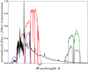	Fig. 1. Transmission curves of the filters used in this work. Blue lines: SDSS-u and SDSS-r filters; red lines: the Pan-STARRS1 filter set: g_PS, r_PS, i_PS, z_PS, y_PS; green lines: Spitzer/IRAC [3.6 μm] and [4.5 μm] bands; purple lines: WISE W1 and W2 bands; and the solid black line shows a simulated quasar spectrum from our library at z = 3.4 (see Sect. 6.2).
Open with DEXTER

As a first step to obtaining mid-infrared photometry for the spectroscopic quasars, we combined the observations from all deep Spitzer/IRAC surveys including: XFLS (Lacy et al. 2005), SERVS (Mauduit et al. 2012), SWIRE (Lonsdale et al. 2003), S-COSMOS (Sanders et al. 2007), SDWFS (Ashby et al. 2009), SHELA (Papovich et al. 2016), and SpIES (Timlin et al. 2016). We followed the same procedure described by Richards et al. (2015) to combine all the Spitzer/IRAC observations. The final catalog contains over 6.2 million Spitzer/IRAC sources. In cases where an IRAC source has been observed multiple times, we used only the deepest IRAC observation.

The mid-infrared photometry for spectroscopic quasars outside the footprint of Spitzer/IRAC surveys comes from observations by NASA’s Wide Infrared Survey Explorer (WISE, Wright et al. 2010). WISE mapped the sky at 3.4, 4.6, 12 and 22 μm (known as W1, W2, W3, and W4). After the cryogenic fuel of the satellite was exhausted in 2010, WISE continued its observations as part of the post-cryogenic NEOWISE mission phase using only its two shortest bands (W1 and W2). We used the SDSS/unWISE forced photometry catalog by Meisner et al. (2017). This catalog provides forced photometry of custom WISE coadds, at the positions of over 400 million SDSS primary sources. This approach provides WISE flux measurements for sources blended in WISE coadds, but resolved in SDSS images and non-detected objects below the “official” WISE magnitude limits (i.e., ALLWISE; Cutri 2013). We only used the W1 and W2 bands as the other two bands are shallower and, thus, have lower detection rates.

We retrieved the SDSS, Pan-STARRS1, and WISE photometry from the SDSS database via CasJobs² and the Mikulski Archive for Space Telescopes (MAST) with PS1 CasJobs³. We made sure that the objects in our samples had clean photometry by excluding sources with the SDSS bad photometry flags described in Richards et al. (2015). However, we opted to keep objects with the flag BLENDED, as high-z quasars could be flagged as BLENDED in some instances, despite being isolated objects (e.g., McGreer et al. 2009). Only PRIMARY sources were selected from the SDSS data. The flags that describe the quality of the Pan-STARRS1 sources are taken from Table 2 in Magnier et al. (2016). For SDSS and Pan-STARRS1, we use PSF magnitudes, and adopt the w1mag and w2mag columns from the unWISE catalog as the WISE measurements for the W1 and W2 bands, respectively. These WISE magnitudes are converted to AB units using the relations: W1_AB = W1_Vega + 2.699 and W2_AB = W2_Vega + 3.339⁴. We considered only WISE sources that met the following criteria: w1_prochi2 ≤ 2.0 && w2_prochi2 ≤ 2.0 (to avoid sources with low-quality profile fittings) and w1_profracflux ≤ 0.1 && w1_profracflux ≤ 0.1 (to exclude sources with fluxes severely affected by bright neighbors). The SDSS cMODELMAG⁵ magnitudes were also retrieved to investigate the separation of point and extended sources (Sect. 5). The SDSS magnitudes in the u filter, originally in inverse hyperbolic sine magnitudes (Lupton et al. 1999), were converted to the AB system using u_AB = u_SDSS − 0.04 (Fukugita et al. 1996). The WISE-W1 and WISE-W2 photometry was converted to the IRAC 3.6 μm and 4.5 μm bands, respectively, using the transformations derived by Richards et al. (2015). We crossmatched the WISE and Spitzer/IRAC catalogs using a radius of 2″. If the crossmatch was positive, we kept only the IRAC measurement. The SDSS, Pan-STARRS1 and IRAC magnitudes were corrected for Galactic extinction using the prescription by Schlafly & Finkbeiner (2011). Figure 1 shows the transmission curves of the filters utilized in this work.

2.3. Spectroscopic quasars with optical and mid-infrared photometry

To efficiently discover new quasars using ML techniques, requires the compilation of a large and representative sample of spectroscopic quasars (e.g., Richards et al. 2015; Pasquet-Itam & Pasquet 2018; Jin et al. 2019). For this purpose, we used the Million Quasars (Milliquas) catalog v6.2 2019⁶ by Flesch (2015). This catalog contains more than 600 000 type-I quasars and active galactic nuclei (AGN) from the literature, and is updated on a regular basis. The majority of quasars included in the Milliquas catalog were discovered as part of SDSS/BOSS (Schneider et al. 2010; Pâris et al. 2018), LAMOST (Yao et al. 2019), ELQS (Schindler et al. 2017), 2QZ (Croom et al. 2004), 2SLAQ (Croom et al. 2009b), and many other surveys (e.g., Papovich et al. 2006; Trump et al. 2009; Kochanek et al. 2012; Maddox et al. 2012; McGreer et al. 2013). We only considered quasars with magnitudes measured for each band to maximize the use of the multi-dimensional color information available.

3. Classification

In this section, we explain how the training and target (objects to be classified) samples were compiled and the different algorithms used for the classification of quasars in the NDWFS-Boötes field. We also assess the performance of the classification algorithms by calculating their efficiency and completeness.

3.1. Training sample

A critical success factor for any ML technique to classify astronomical sources is the use of an appropriate training sample to identify new objects in the target sample. The training sample must have measurements in the relevant filters to identify the characteristic spectral features (e.g., colors) of the sources of interest (e.g., quasars) in order to map their parameter space. At the same time, the training sample has to be representative of the target data. This means not only including a significant number of the sources of interest, but also the other types of astronomical objects expected to be part of the target sample (i.e., stars and galaxies). In particular for quasars, the training samples require several thousands of these objects to robustly extract their color trends as a function of redshift (Yèche et al. 2010; Richards et al. 2015; Nakoneczny et al. 2019; Pasquet et al. 2019). Unfortunately, there are only 2042 quasars with 0.126 ≤ z ≤ 6.12 in the NDWFS-Boötes field, with only 1259 of these quasars having redshifts larger than 1.4 (Flesch 2015). The Boötes quasars in this catalog are drawn mainly from the AGN and Galaxy Evolution Survey (AGES, Kochanek et al. 2012), but other quasar surveys (Cool et al. 2006; McGreer et al. 2006; Glikman et al. 2011; Pâris et al. 2018) have been used as well. These objects are included in the Milliquas catalog (Flesch 2015). However, this sample is too small and sparse, to properly map the parameter space of quasars in the NDWFS-Boötes field. Instead of relying only on the NDWFS-Boötes quasar sample to identify new quasars, we created a training sample using as starting point the Milliquas catalog presented in Sect. 2.3.

We restricted the redshift range of our analysis to 1.4 < z < 5.0 for the following reasons. First, the host galaxies of some z < 1 quasars can be detected in the NDWFS images. This implies that the contribution of the host galaxy component to the overall quasar spectra has to be considered for these sources. This makes it difficult to separate low-z galaxies and quasars using morphological classification based on standard photometric criteria. Secondly, low-z contaminants, such as star-forming, blue, and emission-line galaxies, can mimic the colors of high-z quasars due to their 4000 Å breaks (Smith et al. 1993; Richards et al. 2002). Therefore, we set the lower redhift limit to z = 1.4. This choice is a compromise between reducing contamination by galaxies and excluding good candidate quasars from the sample, but ensures that the degree of contamination due to galaxies across the redshift interval considered is as low as possible. Thirdly, at redshifts z > 5 the number of known quasars is significantly low compared with lower redshifts. Thus, we set z = 5.0 as the upper redshift limit for our analysis. In the training sample, we included spectroscopic quasars with redshifts slightly larger than the redshift limits of our analysis. This helps to reduce the possibility of quasars located at the edges of the redshift intervals not being identified by the classification algorithms. Therefore, we included spectroscopic quasars with 1.2 ≤ z ≤ 5.5 in our training sample.

The first step to create our training sample is to crossmatch the entire Milliquas catalog with the SDSS, Pan-STARRS1, WISE, and IRAC surveys as described in Sect. 2.2. Only objects with a spectroscopic confirmation as quasars are considered. We made sure that the quasars in the training sample have clean photometry by excluding quasars with SDSS, IRAC, and WISE bad photometry flags (see Sect. 2.2). We limited the spectroscopic quasar sample to magnitudes 16.0 ≤ i_PS ≤ 23.0 as this range contains 99.9% of all optical/mid-infrared quasars in the training sample. In total, our sample contains 32 8956 spectroscopic quasars with 1.2 ≤ z ≤ 5.5. These quasars have clear photometry and are detected in the optical and near-infrared (u, g_PS, r_PS, i_PS, z_PS, y_PS), and mid-infrared (3.6 μm, 4.5 μm) bands considered in our analysis. These objects are assigned the label “quasar” in our training sample. This label assignment could be seen as trivial, but it is fundamental because the algorithms introduced in Sect. 3.3 require labels to categorize new unlabeled data in the target sample.

The rest of the training sample that comprises non-quasar objects was compiled as follows. First, we needed to consider that the target sample does not only contain 1.2 ≤ z ≤ 5.5 quasars, but ones with redshifts lower than 1.2 as well. Thus, to ensure that the training sample was representative, we included quasars with redshifts 0 ≤ z < 1.2 from the Milliquas catalog. There is a total of 71 830 quasars that were selected as described in Sect. 2.2, and were assigned the “non-quasar” label. Secondly, stars and galaxies were expected to be part of the target sample. We included them in the training sample by randomly drawing objects with clean photometry (see Sect. 2.2) from the SDSS database with CasJobs, and excluding sources located in the NDWFS-Boötes region. These objects have m_AB < 15 in all the bands to avoid saturated pixels, and must have been classified spectroscopically as stars or galaxies by the SDSS pipeline. If the source was matched within a radius of 2″ to a known spectroscopic quasar it is excluded. We did not apply any morphological criteria to the sources added to the training sample. The drawing process was repeated until a total of 1 098 858 “non-quasar” objects are selected. This size was chosen to have, in combination with the spectroscopic quasar sample, a total of a million and a half of objects in the training sample. The inclusion of galaxies, stars, and z < 1.2 quasars in the training sample is important because it helps the classification algorithms to delimit the color space of “quasars” and “non-quasars”. The details of the training sample are summarized in Table 1.

Table 1.

Properties of the training and target samples.

3.2. Target sample

The target sample is the Spitzer/IRAC-3.6 μm matched catalog presented in Sect. 2.1. As mentioned in Sect. 3.1, there is deep optical photometry available for the NDWFS-Boötes field in the U_spec, B_W, R, I, Z_Subaru bands, however, the number of quasars with photometry in these bands is small. Fortunately, the entire NDWFS-Boötes field is located inside the SDSS/Pan-STARRS1 footprint, and thus photometry from these surveys is available for the target sample. We obtained SDSS and Pan-STARRS1 photometry for all the objects in the NDWFS-Boötes catalog following the same procedure as for the training set. We removed sources with m_AB ≥ 15 in all the bands (SDSS, Pan-STARRS1, IRAC) regardless of their flags to avoid saturated pixels. We kept only sources with the SDSS/Pan-STARRS1 good photometry flags. We had also considered using the IRAC flags (SExtractor flags indicating possible blending issues in the source extraction) but found that around 60% of the z > 1.4 spectroscopic quasars in Boötes are flagged. Considering that the removal of such a significant fraction of quasars from the analysis could affect our conclusions, we decided not to remove flagged IRAC sources from the target sample at this point. In Sects. 3.3.5 and 4.3, we confirmed that including sources marked by the IRAC flags does not result in a deterioration of the quality of the classification, and determination of the photometric redshifts. Finally, the details of the target sample are summarized in Table 1.

3.3. Classification algorithms

In supervised ML, classification algorithms rely on labeled input data (training sample) to produce an inferred function, which can be used to categorize new unlabelled data (target sample). If there is a strong correlation between the input data and the labels a robust inferred function can be obtained. This usually results in a better performance of the ML classification algorithms. In this work, our aim is to identify new quasars in the NDWFS-Boötes field in the target sample using supervised ML classification algorithms. For quasars, the obvious choice is to use their colors for classification purposes (e.g., Richards et al. 2002, 2009, 2015; Timlin et al. 2018). Therefore, we used the color indices (u − g_PS, u − r_PS, g_PS − r_PS, r_PS − i_PS, i_PS − z_PS, z_PS − y_PS, y_PS − [3.6 μm], [3.6 μm] − [4.5 μm]) of the training and target samples as inputs to the classification algorithms. The algorithms used in our analysis (Random Forest, Support vector machine, and Bootstrap aggregation) were selected because of their extensive use in previous studies of quasars (e.g., Gao et al. 2008; Peng et al. 2012; Carrasco et al. 2015; Timlin et al. 2018; Jin et al. 2019). Each one of these algorithms is briefly explained below. They are also part of the open-source scikit-learn⁷ Python library.

3.3.1. Random forest

A random forest (RF, Breiman 2001) ensemble is composed of random decision trees, with each one created from a random subset of the data. The outputs of the decision trees are combined to make a consensus prediction. The final RF classification of an unlabeled instance is determined using the majority vote of all decision trees.

3.3.2. Support vector machines

The support vector machines (SVM, Cortes & Vapnik 1995) is a discriminative classifier for two-group problems. The basic idea is to find an optimal hyperplane in an N-dimensional space (N is the number of features) that distinctly categorizes the data points. In two dimensions, the hyperplane is a line dividing the parameter space in two parts wherein each group is located on either side. For unlabeled instances, the SVM classifier outputs an optimal hyperplane which is used to classify them.

3.3.3. Bootstrap aggregation on K-nearest neighbors

Bootstrap Aggregation (Breiman 1996), also called bagging, is a method for generating multiple versions from a training set, by sampling the original sample uniformly and with replacement. Subsequently, each one of these subsets is used to train the K-Nearest Neighbors algorithm (KNN, Altman 1992). In the KNN algorithm, an unlabelled object is classified by a simple majority vote of its neighbors, with the object being assigned the label most common among its k nearest neighbors (k is a positive integer). In the case k = 1, the label assigned is of that of the single nearest neighbor. For each bagging subset, we use a value of k = 50. Finally, the results of the bagging subsets are aggregated by averaging to obtain a final classification.

3.3.4. Performance

We assessed the performance of the classification algorithms with the quasar training sample presented in Sect. 3.1, by calculating their completeness and efficiency.

The completeness C (Hatziminaoglou et al. 2000; Retana-Montenegro & Röttgering 2018) is defined as the ratio between the number of quasars correctly identified as quasars, and the total number of quasars in the sample:

(1)

The efficiency E is defined as the ratio between the number of quasars correctly identified as quasars, and the total number of objects identified as quasars:

(2)

As is common practice in supervised ML, the training sample described in Sect. 3.1 is separated into validation and test samples for cross-validation (CV) purposes, in order to calculate the performance on observations of the classification algorithms. The validation set is used as the training sample, while the CV test sample, which contains spectroscopic quasars, is employed to report the completeness and efficiency of the classification algorithms. As the CV test set, we chose a random 25% subsample of the full training set. The remaining 75% of the training data was the validation sample, and is used to train the algorithms.

In Table 2, we present the completeness and efficiency for all the classification algorithms. While the differences are small, performance of the SVM algorithm is the worst, while RF has the highest completeness and efficiency values.

Table 2.

Performance of the classification algorithms for the quasar training sample.

3.3.5. Classification results

In this section, we discuss the results of the application of the classification algorithms to our target sample. To identify the maximum number of quasars, we combined the results of the three classification algorithms. While this step increases the sample completeness, it also increases the amount of contamination on the sample despite each algorithm having low degree of contamination (see Table 2). In Sects. 3.3.6 and 5, we took additional steps to eliminate contaminants from our quasar sample. At this point, the classification algorithms identified 39 160 objects as quasar candidates. Of these, 36 699 lack spectroscopic observations, and 2470 sources had been classified spectroscopically. By crossmatching our sample with the Milliquas catalog, we found that 1374 are already known quasars. From these quasars, 1042 have redshifts larger than z > 1.4. This corresponds to a completeness of 87% for the sample of Boötes spectroscopic quasars. Additionally, we checked the AGES catalog (Kochanek et al. 2012) and NED⁸ database to find that 1096 objects had been classified spectroscopically as either galaxies or galaxies. The confirmed stars and galaxies were removed from the sample.

3.3.6. Radio data

The contamination by the stars and galaxies in quasar samples is inevitable as they occupy similar regions in the color space used to train the classification algorithms. As has already been discussed, an efficient way to eliminate stellar sources from quasar samples is to include information from radio surveys (Richards et al. 2002; Retana-Montenegro & Röttgering 2018). For this purpose, we used the LOFAR observations of the NDWFS-Boötes field by Retana-Montenegro et al. (2018) introduced in Sect. 2.1. We crossmatched our quasar sample and the LOFAR catalog using a radius of 2″ to identify the spectroscopic quasars detected in our LOFAR mosaic. We also inspected their stacked RGB (R = B_W, G = R, B = I) images with radio contours overlaid to ensure that the match between optical and radio counterparts is correct and to eliminate likely contaminants due to image artifacts or spurious matches still present in our sample. We identified 83 spectroscopic quasars with 5σ LOFAR detections. We identified the photometric quasars in Sect. 5 calculated their photometric redshifts in Sect. 4, and used a morphology cut in the optical as a function of redshift to eliminate extended sources.

4. Photometric redshifts

4.1. Nadaraya–Watson kernel regression

Our sample contains only 83 spectroscopic quasars. For the photometric quasars, we estimated their photometric redshifts z_phot using the Nadaraya–Watson (NW) kernel regression estimator (Nadaraya 1964; Watson 1964). The NW estimator is part of the family of kernel regression methods, in which the expectation of the variable Y relative to a variable X does not depend on all the X-values, as in traditional regression methods, but on sets of locally weighted values. A bandwidth scale parameter determines the amount of local averaging that is performed to obtain the estimate of Y. The NW estimator has been widely applied for nonparametric classification and regression (e.g., Li & Racine 2011; Campbell et al. 2012; Qiu 2013) and to derive photometric redshifts (Wang et al. 2007; Timlin et al. 2018).

The NW estimate is a weighted average of the observed variable y_i calculated utilizing nearby points around the test point x₀. The estimate is calculated using the following equation:

(3)

where

(4)

is the normalized kernel built using the local information from the training sample, and N is the number of objects in the training sample. The kernel weighting function K(x_i,x₀) is chosen to have a Gaussian form:

(5)

where h is the bandwidth scale that defines the region of parameter space in which the data is averaged, and ‖x_i−x₀‖ is the euclidean distance between the data points from the training and test samples. A more detailed discussion about the NW estimator can be found in Härdle (1990) and Wu & Zhang (2006).

In this work, the training sample is composed of spectroscopic quasars, and the distance is calculated between the colors of the spectroscopic quasars and photometric quasars. Finally, for each photometric quasar its photometric redshift is calculated considering all the spectroscopic redshifts of the training sample by using the equation (Wang et al. 2007; Timlin et al. 2018):

(6)

4.2. Quasar training sample

To provide a training sample on which to use the NW estimator, a spectroscopic quasar catalog is necessary. For this purpose, we used the quasar catalog introduced in Sect. 2.3. In total, our training set contains 328 956 quasars with 1.2 ≤ z ≤ 5.5 to determine photometric redshifts using the NW estimator (see Table 1).

4.3. Redshift estimation

The distance between the color indices (u − g_PS, u − r_PS, g_PS − r_PS, r_PS − i_PS, i_PS − z_PS, z_PS − y_PS, y_PS − [3.6 μm], [3.6 μm] − [4.5 μm]) of the spectroscopic quasars from the training sample and the corresponding photometric objects are used as inputs to build the kernel matrix as given in Eq. (5). An important decision in building the kernel is the choice of the bandwidth scale h. With smaller values of h nearby data points have more weight, while larger values of h result in an increasing contribution of distant data points. Finally, the kernel functions determined using Eq. (6) are used as weights in the computation of the photometric redshift.

The quality of the photometric redshifts determined with the NW estimator is investigated utilizing two quasar samples. The first sample is composed of 1193 quasars from the quasar training set described in Sect. 2.3 that are located in the NDWFS-Boötes field. The second sample is a subsample selected randomly from the training set. We measure the performance of the photometric redshifts in the samples using the following statistics:

– mean of the difference between photometric and spectroscopic redshifts, ⟨△z⟩ = ⟨(z_phot−z_spec)⟩, unclipped;

– standard deviation of the △z, σ(△z);

– fraction of quasars with |△z| < 0.3, R_0.3;

– mean of normalized △z, ⟨△z_norm⟩ = ⟨(z_phot−z_spec)/(1+z_spec)⟩, unclipped;

– standard deviation of the normalized bias, σ(△z_norm);

– fraction of quasars with |△z_norm| < 0.1 (|△z_norm|< 0.2), ().

These results are summarized in Table 3. We tested practically all the values in the range 0.01 ≤ h ≤ 0.5, and found that h = 0.09 gives the best performance and least scatter for the Boötes spectroscopic quasars (see Table 3). This h value is slightly higher than the h = 0.05 used in previous estimations of photometric redshifts using the NW estimator (e.g., Wang et al. 2007; Timlin et al. 2018). Figure 2 shows the photometric versus spectroscopic redshifts for the spectroscopic sample of Boötes quasars. At low-z, the dispersion of the photometric is slightly higher in comparison with the high-z estimations. This is expected as at low-z there are less spectral features for the NW method to exploit and predict trends on the training sample.

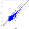Fig. 2.

Photometric z_photo versus spectroscopic z_spec redshift for spectroscopic quasars in the NDWFS-Boötes region. The photometric redshifts are obtained using the NW kernel regression. The grey line indicates the one-to-one z_NW = z_spec relation, and the dashed-dotted and dashed lines indicate the z_NW − z_spec = ±0.10 × (1 + z_spec) and z_NW − z_spec = ±0.20 × (1 + z_spec) relations, respectively.

Open with DEXTER

Table 3.

Performance of the photometric redshifts for the quasar training sample.

Figure 3 presents the normalized histogram of the bias △z = z_phot − z_spec between photometric and spectroscopic redshifts for the different experiments listed in Table 3. The first row lists the result for the sample of Boötes quasars. This shows that the majority of Boötes quasars have good redshift estimations. The number of outliers is small with 76% of the quasars having photometric redshifts that do not differ more than |△z| ≤ 0.3 from their spectroscopic redshifts. A good comparison for the redshift accuracy of the Boötes quasars can be obtained using a validation sample that is randomly selected from a training sample. This validation sample contains 65 573 quasars, and its size is 20% of the total training sample. The result for this sample is listed in the last row of Table 3. The Boötes sample performs worse than the 20% of the training sample in terms of bias, scatter, and fractions of quasars with correct redshifts. In order to better understand the reasons for the difference in performance between the two samples we examine the performance of the NW method as a function of the photometric errors in the SDSS/Pan-STARRS1 bands. By restricting the Boötes sample only to quasars with photometric errors in the SDSS/Pan-STARRS1 bands smaller than err ≤ [0.2, 0.3, 0.5], respectively, its performance gets closer to that of the 20% training sample, and this further improves for the case when the photometric errors are smaller or equal to 0.3 (Table 3, third-fourth rows).

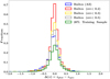	Fig. 3. Normalized histogram of the bias △z = z_phot − z_spec between photometric and spectroscopic redshifts for different samples. The phometric redshifts are obtained using the NW kernel regression. Around 76% of the spectroscopic quasars in the Boötes field have photometric redshifts that are correct within \|△z\| = 0.3 (see Table 3).
Open with DEXTER

Finally, we compared the performance of the NW regression kernel with other photometric-redshift algorithms. For instance, Richards et al. (2001) and Weinstein et al. (2004) reported that 70% and 83% of their predicted photometric redshifts are correct within |δz| ≤ 0.3. These authors used empirical methods that used the color-redshift relations to derive photometric redshifts using early SDSS data. Yang et al. (2017) considered the asymmetries in the relative flux distributions of quasars to estimate quasar photometric redshifts obtaining an accuracy of for SDSS/WISE quasars. Jin et al. (2019) employed the SVM and XGBoost (Chen & Guestrin 2016) algorithms to achieve an average accuracy of for the photometric redshifts of their Pan-STARRS1/WISE quasars. Schindler et al. (2017) used SDSS/WISE adjacent flux ratios to train the RF and SVM methods to obtain average results of for their photometric redshifts. In summary, despite the fact that all these algorithms employed different samples and redshift intervals, their accuracy is consistent with the results obtained in this work using the NW regression kernel. Finally, it is also important to mention that the reason for using the NW regression is its better performance for our quasar sample in comparison with other ML methods. For example, the RF regression underperforms in all the statistics indicated in Table 3. Using the RF estimator, for the Boötes spectroscopic quasars (the all sample in Table 3) we obtained less accurate photometric redshifts with R_0.3 = 0.70 and . Therefore, we calculated our photometric redshifts using the NW regression kernel.

5. Quasar sample

5.1. Final sample

We used the NW regression algorithm to assign a photometric redshift to each photometric quasar detected by LOFAR. To eliminate potential contamination by low-z galaxies, we restricted our quasar sample only to point sources. The SDSS photometry pipeline⁹ classifies an object as point-like (star) or extended (galaxy) source based on the difference between its PSF and cMODELMAG magnitudes¹⁰. Various methods have been proposed to perform the morphological star-galaxy separation with photometric data by adding Bayesian priors to the aforementioned magnitude differences (Scranton et al. 2002), and using decision tree classifiers (Vasconcellos et al. 2011). Here we employed a criterion derived directly from the Boötes spectroscopic quasars by considering the difference △_mag between the PSF and cMODELMAG magnitudes in the SDSS-r band as a function of redshift. Spectroscopic quasars were binned according to their redshifts to calculate the magnitude difference as the quantile that contains 95% of the quasars in the corresponding bin. The redshift intervals match those utilized to derive the luminosity function in Sect. 6.4. Objects with magnitude differences less than the △_mag value in their corresponding redshift bin were considered to be point sources, and are included in our RSQs sample. Figure 4 shows the magnitude differences as a function of redshift. Finally, we restricted our RSQs sample to magnitudes of 16.0 ≤ i_PS ≤ 23.0 to avoid extrapolation beyond the range of the quasar training sample (see Table 1). The resulting catalog consists of 17 924 objects, with 104 sources having a LOFAR counterpart within a radius of 2″.

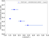	Fig. 4. Difference between the `PSF` and `cMODELMAG` magnitudes in the r band to separate point-like and extended sources as a function of redshift. The difference values are calculated considering the quantile that contains 95% of the quasars in the corresponding redshift bin. The redshift intervals match those used to derive the luminosity function in Sect. 6.4.
Open with DEXTER

After the morphological cut, we carefully inspected the false-color RGB images (R = B_W, G = R, B = I) of the photometric quasars detected with ≥5σ significance in the LOFAR mosaic overlaid with radio contours to reject blended sources, artifacts, and spurious matches to the radio data. The majority of discarded sources corresponded to objects that are spurious matches to the LOFAR data. The final RSQs catalog resulting from our selection contains 47 photometric quasars and 83 spectroscopic quasars. In Fig. 5, it can be seen that the colors of the photometric quasars agree well with those of the z > 1.4 quasars in the training and NDWFS-Boötes quasar samples. The importance of the use of the LOFAR data is clear as it allows for a significant reduction in the number of stellar contaminants in the sample of objects taken as quasars by the ML algorithms. The initial sample is reduced from ∼18 000 objects to only 47 RSQs detected at ≥5σ significance in the LOFAR mosaic. This represents a reduction of two orders of magnitude in the number of contaminants.

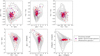Fig. 5.

Comparison between the colors of the training and NDWFS-Boötes (photometric and spectroscopic quasars) samples. Black contours and points denote the spectroscopic quasars with z > 1.4 of the training sample, while purple squares indicate all the spectroscopic quasars in Boötes with z > 1.4. Photometric quasars in our sample are denoted by red circles. The training sample is employed to identify quasars in the target sample (see Sect. 3), and to determine their photometric redshifts with the NW kernel regression method (see Sect. 4.1).

Open with DEXTER

In Fig. 6, we compare the colors of the photometric quasars with those of the training sample and Boötes spectroscopic quasars as functions of redshift. The color-redshift spaces occupied by photometric RSQs are in good agreement with those of Boötes spectroscopic quasars and the quasar training sample. Figure 7 displays the redshift distribution of photometric and spectroscopic quasars. At z ≲ 2.8, the majority of the quasars in our sample are spectroscopic. Considering that 77% of the photometric quasars have photometric errors smaller than err ≤ 0.5, we conclude that the accuracy of their photometric redshifts is similar or slightly worse to that of the Boötes sample with photometric errors that are err ≤ 0.5 (see Table 3). The i_PS-band magnitude and 150 MHz flux distributions of the RSQs sample are presented in Fig. 8, while the absolute magnitude and radio luminosity are displayed in Figs. 9 and 10, respectively. The absolute magnitudes are calculated using the K-correction discussed in Sect. 6.2. The majority of RSQs (130 in total) in our sample are unresolved or resolved into single-component radio sources in the LOFAR-Boötes mosaic with a resolution of ∼5″. In our sample, only 11 quasars present radio-morphologies consistent with a core-jet structure. Appendix A presents a selection of false-color RGB images of spectroscopic and photometric RSQs from our final sample. The catalogs of spectrocospic and photometric RSQs are only available at the CDS.

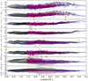	Fig. 6. Quasar colors versus redshift for different quasar samples between z = 1.4 and z = 5.5. Red points: RSQs with photometric redshifts; purple points: Boötes spectroscopic quasars; black contours and points: color distributions of the quasar training sample from Sect. 2.3; blue lines: mean color–redshift relations derived from the quasar training sample.
Open with DEXTER

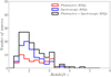	Fig. 7. Redshift distribution of photometric (red) and spectroscopic (blue) RSQs. Also, the combined redshift distribution (black) of photometric and spectroscopic RSQs is plotted.
Open with DEXTER

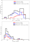	Fig. 8. i_PS (top) and total flux S_150 MHz (bottom) distributions of photometric (red) and spectroscopic (blue) RSQs. Also, the combined redshift distribution (black) of photometric and spectroscopic RSQs is plotted. The method employed to select the quasars is described in Sect. 3.3.
Open with DEXTER

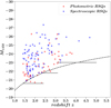Fig. 9.

Absolute magnitude M₁₄₅₀ versus redshift for photometric (red) and spectroscopic (blue) RSQs in our sample. To minimize incompleteness due to incomplete M₁₄₅₀ bins while retaining the maximum numbers of quasars for estimating the luminosity function, we consider only RSQs with M₁₄₅₀ ≤ [−20.6,−21.8,−23.0] at 1.4 ≤ z < 2.4, 2.4 ≤ z < 3.1, and 3.1 ≤ z < 5.0; respectively. The dashed line denotes the magnitude limit i_PS = 23.0. This limit is calculated assuming a quasar continuum described by a power-law with slope α = −0.5 with no emission line contribution or Ly_α forest blanketing.

Open with DEXTER

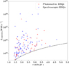	Fig. 10. Rest frame absolute luminosity density at 150 MHz versus redshift for photometric (red) and spectroscopic (blue) RSQs in our sample. The solid line denotes the 5σ flux limit (275 μJy) of the Boötes observations presented by Retana-Montenegro et al. (2018).
Open with DEXTER

5.2. Spectral energy distribution of photometric quasars

In this section, we used the deep photometry available in the NDWFS-Boötes field to calculate the spectral energy distributions (SEDs) of the photometric quasars. This additional deep photometry provides an additional piece of information to confirm the validity of the photometrically selected sources selected using the ML algorithms as robust candidate quasars. For this purpose, we used the I-band matched photometry catalog presented by Brown et al. (2007). The 5σ limiting AB magnitudes for the relevant filters are provided in Table 4. Each filter image was convolved to a common pixel scale, so that all the point spread functions (PSFs) images matched a Moffat profile. In these images, photometry was computed with SExtractor (Bertin & Arnouts 1996) using the I-band as the detection band. This catalog contains more than two millions of I-band selected sources.

Table 4.

Characteristics of the filters used in the NDWFS-Bootes field and their 3σ AB limiting magnitudes.

For each object, the goodness-of-fit, χ², is estimated through the fitting of the object’s photometric data to a SED quasar template. We used a compilation of quasar templates from the literature. This includes the composite quasar templates by Cristiani & Vio (1990), Vanden Berk et al. (2001) and Gavignaud et al. (2006), respectively; and the type-1 quasar templates by Salvato et al. (2009) (pl_I22491_10_TQSO1_90, pl_QSOH, pl_QSO_DR2, pl_TQSO1). To account for dust extinction in the quasar hosts, we modify the quasar templates using the Calzetti et al. (2000) starburst, Pei (1992) Small Magellanic Cloud (SMC), and the Czerny et al. (2004) extinction laws. The extinction was applied to each template according to a grid E(B − V) = [0.0, 0.05, 0.1, 0.15, 0.2, 0.25, 0.3, 0.4, 0.5]. We performed these fittings using the photometric redshift code EAZY (Brammer et al. 2008). For all the SED libraries, the zero points were calculated using the standard procedure of fitting the observed SEDs of a sample of spectroscopic objects, fixing their redshift to the known spectroscopic redshift (see Ilbert et al. 2006 for more details). The spectroscopic sample used to determine the zero points are the NDWFS-Boötes quasars with z ≥ 1.4. Due to the large number of templates in the quasar template library, only single template fits were considered. Figure 11 shows the SED fitting to four photometric quasars in our sample. There is a good agreeement between the NDWFS-Boötes photometry and the quasar templates. Figure 12 displays the distribution of the reduced goodness–of-fit values, , where N is the number bands in which the quasar is detected, for NDWFS-Boötes spectroscopic and photometric quasars. We determined the probability that both samples are from the same parent population by doing a Kolmogorov–Smirnov (K–S) test. The K–S test indicates that there is a probability of 27% that both samples are being drawn from the same distribution. Thus, we cannot reject the hypothesis that the distributions of the two samples are the same. This hypothesis also cannot be rejected if the K–S test is applied to the redshift distributions. In this case, we found that the hypothesis cannot be rejected at the 95% level.

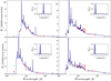Fig. 11.

Spectral energy distributions (SEDs) of four photometric quasars identified using our ML algorithms (see Sect. 3.3). The NDWFS-Boötes photometry is used to calculate the SEDs. In each case the best-fit quasar template (as derived from the EAZY calculation) is also plotted. Red circles are the photometric points and the blue circles indicate the predicted photometry by the best-fit template. The probability density distributions (PDFs) for each object are shown in the small inset. These PDFs strongly suggest that these objects are quasars located at z > 1.4.

Open with DEXTER

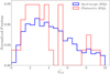	Fig. 12. Normalized distributions of all NDWFS-Boötes spectroscopic quasars with z ≥ 1.4 (blue) and photometric (red) RSQs. See Sect. 5.2 for more details.
Open with DEXTER

5.3. Cross-matching to X-ray data

Our quasar sample was correlated with the 5 ks deep Chandra catalog of the NDWFS-Boötes field XBoötes (Kenter et al. 2005) using a 2″ matching radius. A total of 44 spectroscopic quasars and 6 photometric quasars are detected by the Chandra satellite. The high detection fraction of spectroscopic quasars is not unexpected, as a X-ray detection in the XBoötes catalog was one of the criteria used for spectroscopic follow-up of AGN candidates in the AGES survey (see Kochanek et al. 2012, Sect. 2). In conclusion, deeper X-ray exposures are required to detect the rest of the quasars in our sample.

5.4. Density of photometric quasars

In this section, we compare the density of photometric quasars in our sample with previous works. After the morphological cut, but before cross-matching with the LOFAR catalog the density of our sample is of 1927 photometric quasars per square degree. This number could be considered high in comparison with previous results. For example, Richards et al. (2015) using a Bayesian kernel density algorithm found a surface density of ∼51 optical/mid-infrared photometric quasars per square degree. Jin et al. (2019) employed the XGBoost and SVM classification algorithms to obtain a density of ∼38 Pan-STARRS/WISE photometric quasars per square degree. Both works considered similar ranges in optical magnitude and redshift. Two reasons can explain our higher density of photometric quasars. Firstly, we do not restrict our mid-infrared photometry using any quality flag (only limiting the sample to objects with m_AB ≥ 15), as is done in the aforementioned works. Secondly, our relatively deep mid-infrared observations were obtained with Spitzer/IRAC, while the majority of mid-infrared imaging used by Richards et al. (2015) comes from shallower WISE observations, and Jin et al. (2019) employed only WISE data. Hence, it is only for the purposes of comparison in this section that we restricted our sample only to photometric quasars detected in WISE, and keep only those that fulfill the WISE photometry flags used in Richards et al. (2015). This reduced sample contains 538 objects detected by WISE, which corresponds to a density of ∼58 photometric quasars per square degree. This density is in agreement with the aforementioned works, and the reason for the apparent difference in the number of photometric quasars is the depth of the IRAC imaging, and our treatment of the quality flags of the IRAC photometry.

5.5. LOFAR and wedge-based mid-infrared selection of quasars

In this section, we compare the LOFAR and wedge-based mid-infrared selection (Stern et al. 2005) for objects classified as quasars by the ML classification algorithms. Firstly, we used the mid-infrared color cuts proposed by Lacy et al. (2007) and Donley et al. (2012) to identify the presence of AGN-heated dust in our photometric RSQs. Figure 13 shows the mid-infrared colors for different quasar samples in the NDWFS-Boötes field. The mid-infrared colors of the photometric RSQs are in good agreement with those of spectroscopic quasars, and the majority of both spectroscopic and RSQs are located within the region delimited by the Donley et al. (2012) color cuts. To be exact, 89.93% (70.59%) of the 1192 (47) spectroscopic quasars (photometric RSQs) with redshifts z > 1.4 are located within the region delimited by the Donley et al. (2012) color cuts, 98.15% (94.12%) reside in the region common to the Lacy et al. (2007) and Donley et al. (2012) color cuts, and only 1.85% (5.88%) are located outside the boundaries delimited by the aforementioned wedge-based mid-infrared color cuts. Considering the following points regarding our photometric RSQs: (i) these objects are identified as quasar by the ML algorithms; and (ii) their optical and mid-infrared colors are similar to those of spectroscopic quasars. We are confident, therefore, that our sample of photometric RSQs is composed mainly of real quasars and the number of contaminants is minimal. Moreover, these points show that utilizing ML algorithms trained using optical and infrared photometry and combined with LOFAR data is a very efficient and robust way to identify quasars.

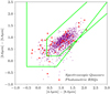	Fig. 13. Mid-infrared colors for photometric and spectroscopic quasars in the Boötes field. The photometric RSQs are plotted as red circles, while the spectroscopic quasars are indicated by purple circles. The light green lines are the mid-infrared color cuts proposed by Lacy et al. (2007) and Donley et al. (2012).
Open with DEXTER

To investigate the wedge-based mid-infrared selection of quasars without radio detections, we first needed to establish the nature of these objects as robust quasars candidates or contaminants (i.e., stars or galaxies). For this purpose, we followed a classification method based on the goodness–of-fit, χ², estimated through the fitting of the object’s photometric data to a given type of SED template (quasar, galaxy, and stellar) (e.g., Ilbert et al. 2006; Masters et al. 2015). This fitting assigns to each object three χ² values: , , and , which corresponds to the fitting of the object photometry against the quasar, galaxy, and stellar templates, respectively. In the SED fittings, we utilize only the SDSS, Pan-STARRS1, and IRAC 3.6 μm/4.5 μm bands as this was the photometry used to classify them originally as quasars by the ML algorithms. This also represents a scenario where there is SDSS, Pan-STARRS1, and LOFAR coverage, but shallow or incomplete mid-infrared data to perform a wedge-based mid-infrared selection of faint quasars (e.g., Stern et al. 2005; Messias et al. 2012). The three template libraries used in this analysis are as follows. For the galaxy library, we use the latest version of the Brammer et al. (2008) SED templates that include nebular emission lines; while for the star library we select the Chabrier et al. (2000) SED templates. For the quasar template set, we use a compilation of quasar templates from the literature. This includes the composite quasar templates by Cristiani & Vio (1990), Vanden Berk et al. (2001) and Gavignaud et al. (2006), respectively; and the type-1 quasar templates are the same as those used in Sect. 5.2. To account for dust extinction in the galaxies, we modified the galaxy templates using the Calzetti et al. (2000) starburst and Pei (1992) Small Magellanic Cloud (SMC) extinction laws using a E(B − V) grid (see Sect. 5.2). The spectroscopic samples used to determine the zero points are the quasars, galaxies, and stars of the training sample presented in Sect. 3.1. We compute the χ² values using the photometric redshift code EAZY (Brammer et al. 2008), as described in Sect. 5.2. From the χ² distribution of spectroscopic quasars in Boötes, we defined empirical χ² cuts to separate quasars from stars and galaxies. Figure 14 displays the comparison of the χ² values resulting from the quasar, galaxy, and star template fitting to the photometry of spectroscopic and photometric quasars in the NDWFS-Boötes field. We found that the empirical cuts , and select the majority of quasars and reject an important fraction of likely stars and galaxies. Based on the cuts described before, we selected 957 out of a total of 1193 spectroscopic quasars; and 4935 of 17 829 photometric quasars. From these, 1423 photometric quasars are found to be located in the region delimited by the Donley et al. (2012) color cuts. The analysis of the mid-infrared selection was limited to the Donley et al. (2012) wedge as it is expected that the majority of quasars will be located within this region. Next we compare the number of photometric quasars selected by the Donley et al. (2012) wedge to the expected number of quasars. The expected number of quasars can be determined using the following expression:

(7)

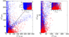	Fig. 14. Comparison of the χ² values for quasar, galaxy, and star template fitting to the photometry of spectroscopic quasars and candidate quasars in the NDWFS-Boötes field.
Open with DEXTER

where A is the survey area, is the quasar luminosity function, and V_c(z) is the comoving volume. We estimated the number of total (radio-detected and undetected) faint quasars using the results by Yang et al. (2018) and Eq. (7). These authors studied the luminosity function of faint quasars between 0.5 < z < 4.5 in a 1.0 deg² field within the VIMOS VLT Deep Survey (Le Fèvre et al. 2013). For redshifts z > 3.5, Yang et al. (2018) did not fit the luminosity function due to the low number of quasars in their sample; therefore, our analysis is limited to the redshift range 1.4 ≲ z ≲ 3.5. According to Yang et al. (2018), the expected number of faint quasars at 1.4 ≲ z ≲ 3.5 in a 9.3 deg² region like the NDWFS-Boötes field is approximately . However, in the redshift range 1.4 ≤ z ≤ 3.5 there are more than 1100 spectroscopic quasars, and 1380 photometric quasars fulfill the Donley et al. (2012) color cuts. Counting only the photometric quasars and not known spectroscopic quasars, the number is higher than the expected number of quasars. This indicates some degree of contamination in the sample of photometric quasars selected using the wedge-based mid-infrared selection. Most likely these contaminants are compact galaxies or AGNs that mimic the colors of quasars, as the majority of stars are expected to be located outside the wedge define by the Donley et al. (2012) color cut. Additionally, comparing these numbers against those of the LOFAR selection, it is likely that there are more contaminants in the wedge-based mid-infrared selected sample than in the LOFAR selected sample. For a case like this, the addition of Euclid (Laureijs et al. 2011) near-infrared imaging (JH bands) in the ML classification process will be useful in eliminating some of these likely contaminants.

The results of this section demonstrated that in the cases where a of lack of deep and complete mid-infrared coverage needed to perform a wedge-based mid-infrared selection of quasars, ML algorithms trained with optical and infrared photometry combined with LOFAR data provide an excellent approach for obtaining samples of quasars. Moreover, considering this and the results obtained in Sect. 5, where with LOFAR data we are not only able to eliminate the stellar contamination in our quasar sample, but also to reduce the number of contaminants by two orders of magnitude. It is clear that the use of LOFAR data to select quasars has a great potential for compiling samples of quasars.

6. Luminosity function of radio-selected quasars

In the following subsections, we describe the steps required to compute the luminosity function of RSQs.

6.1. Selection completeness and accuracy of photometric redshifts

An important step in measuring the luminosity function of quasars is to account (and correct) for the different sources of incompleteness that could bias the quasar counts. In our analysis, we need to consider the completeness of our sample selection and the accuracy of the photometric redshifts. The selection completeness, P_comp(i_PS,z ), is the fraction of quasars that were successfully identified as quasars by the classification algorithms, as function of magnitude i_PS and redshift. P_comp(i_PS,z ) is derived from the data themselves as follows. First, the spectroscopic quasar sample introduced in Sect. 3.1 is binned according to magnitude i_PS and redshift z, in bins of size △i_PS = 0.5, and △z = 0.3, respectively. The quasars in each bin are separated into two subsamples. The first subsample is created by randomly sampling without replacement all quasars in the bin, while the second subsample includes all the quasars that were not sampled. The sizes of the first and second subsamples are 20% and 80% of quasars in the i_PS − z bin, respectively. Having done this for all bins, the corresponding samples are combined to create final training (80%) and target (20%) samples. The final result is the uniform and randomly sampled separation of the training sample into two subsamples in the i_PS − z plane. The main advantage of this binning scheme is that it provides an unbiased and efficient way to map locally the selection completeness obtained using the classification algorithms as a function of magnitude and redshift. The second subsample is used as the training sample for the classification algorithms, while the first subsample has the role of target sample and it is employed to derive the selection completeness. Figure 15 shows the selection completeness, P_comp(i_PS,z ).

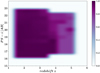	Fig. 15. Selection completeness, P_comp(i_PS,z ), binned according to magnitude i_PS and redshift z, in bins of size △i_PS = 0.5, and △z = 0.3, respectively.
Open with DEXTER

In addition to correcting for selection incompleteness in our sample, we also need to correct for the accuracy of the photometric redshifts determined using the NW regression method. For this purpose, we determine the expected number of spectroscopic quasars to have photometric redshifts correctly and incorrectly assigned within a redshift bin using the NW method. This is done following a similar approach to determining the selection completeness. First, the spectroscopic quasar sample introduced in Sect. 3.1 is divided into the same redshift bins used to derive the luminosity function in Sect. 6.4. In each bin, the quasars contained in that bin are randomly separated to create samples with sizes of 20% and 80% of all quasars in the bin, respectively. The corresponding samples from all the bins are combined to create final training (80%) and target (20%) samples. The training sample is used to train the NW regression method, while the target sample is utilized to determine the expected number of spectroscopic quasars with correctly and incorrectly assigned redshifts within the boundaries of the redshift bins. The ratio between the number of spectroscopic quasars with correctly and incorrectly assigned redshifts, f_photo-z, provides an estimate of the excess of photometric quasars with incorrectly assigned photometric redshifts within a redshift bin (see Fig. 16). This ratio is used as a correction factor for each photometric quasar within the corresponding redshift bin. The derived correction factors have a median factor of f_photo-z ⋍ 1.0, with the 1.65 < z < 2.4 redshift bin having the smallest value with f_photo-z = 0.90.

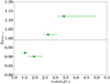	Fig. 16. Ratio between the number of spectroscopic quasars with correctly and incorrectly assigned redshifts, f_photo-z, as a function of redshift. The redshift intervals match those used to derive the luminosity function in Sect. 6.4. The gray dashed line denotes the median value of f_photo-z.
Open with DEXTER

6.2. Simulated Quasar Spectra

In order to calculate the K-correction (see Sect. 6.3), we construct a synthetic quasar library that is an accurate representation of the quasar demography. The variety in the quasar spectral features (UV continuum slope, emission-line EW, and intervening HI absorbers along the line of sight) determine the range in quasar colors. It is important that these spectral features are taken into account to obtain reliable simulated quasar spectra. These spectra are later incorporated into a synthetic quasar library that allow us to compute the K-correction for a given redshift. We explain the procedure followed to build our synthetic quasar library below.

Following several authors (Møller & Jakobsen 1990; Fan 1999; Richards et al. 2006; McGreer et al. 2013), the synthetic quasar spectra are built using a Monte-Carlo (MC) approach. We perform MC simulations to generate quasar spectra adopting a broken power-law (f_λ∝λ^−α_λ) for the UV continuum at 1100 Å. The slope values are drawn from a Gaussian distribution, with mean values of ⟨α_λ⟩ = −1.7 for λ < 1100 Å (Telfer et al. 2002), and ⟨α_λ⟩ = −0.5 for λ > 1100 Å (Vanden Berk et al. 2001), both with standard deviations of σ = 0.30. We bin BOSS quasars by their luminosity to obtain the distribution for the parameters (wavelength, EW, FWHM) of emission lines. This allows us to recover the intrinsic emission line mean and dispersion as function of luminosity, as well as reproducing empirical trends such as the Baldwin effect (Baldwin 1977). We again assume gaussianity when the emission line features are added to the quasar continuum. For each template spectrum, the intergalactic absorption that gives rise to the Ly_α forest is included by creating sightlines in a MC fashion adopting the prescription of neutral absorbers by Bershady et al. (1999). The spectrum is then convolved with our filter passbands to obtain the colors for each synthetic quasar. A Gaussian error is added to the photometry of the mock quasars with a σ derived from the photometric errors of the real magnitudes that match the simulated ones. This error is combined in quadrature with the photometric calibration errors of Pan-STARRS1 (Tonry et al. 2012). In Fig. 1, we show a synthetic spectrum from our quasar library.

6.3. K-correction

Usually, the luminosity functions of quasars are expressed in the absolute magnitude at rest-frame 1450 Å, M₁₄₅₀, which provides a good measurement of the quasar continuum in a region without strong emission lines (e.g., Richards et al. 2006; Croom et al. 2009a; Masters et al. 2012). To derive M₁₄₅₀ for the Boötes quasars, we use the apparent magnitude m_X in a fiducial filter as a proxy:

(8)

where d_L(z) is the luminosity distance in parsecs, and K_X is the K-correction which allows us to convert the magnitudes of distant objects in a given bandpass filter into an equivalent measurement into their rest-frame. Using our synthetic quasar library described in Sect. 6.2, the K-correction can be determined from the difference between apparent magnitudes m_X and m₁₄₅₀,

(9)

with m₁₄₅₀ calculated using a top-hat filter of width 50 Å. Figure 17 displays the K-correction obtained for five different filters, and the expected result from a quasar that has only a power-law continuum and no emission line contribution or Ly_α forest blanketing. The K-correction curves between 1.0 ≤ z ≤ 6.0 are obtained by calculating their average value in redshift bins of size △z = 0.1. At z ≳ 3.7, the difference between the r_PS and i_PS bands becomes more significant as the Ly_α line moves or exits the filters. The same situation occurs at z ≳ 4.7, but for the i_PS and z_PS bands. Therefore, we estimate M₁₄₅₀ using K-corrections selected to minimize any bias caused by the redshifting of the Ly_α emission line. For z < 3.7 quasars, we use a K-correction based on the r_PS band, while for the intervals 3.7 ≤ z ≤ 4.7 and z > 4.7 K-corrections based on the i_PS and z_PS bands, respectively, are employed.

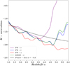Fig. 17.

K-correction for different filters determined using our simulated quasar spectra. The Pan-STARRS1 r_PS and i_PS filters are indicated by blue and green, while the red and cyan are the expected K-corrections for the Pan-STARRS1 z_PS and SDSS-i bands. The solid black line is the K-correction assuming a power-law with slope α = −0.5 with no emission line contribution or Ly_α forest blanketing. At z ≳ 3.7, the difference between the r_PS and i_PS bands becomes more significant as the Ly_α line moves in or out of the filters. The same situation occurs at z ≳ 3.7, but for the i_PS and z_PS bands.

Open with DEXTER

6.4. Quasar Luminosity function

We construct the luminosity functions for all quasars in our radio-matched sample using the classical 1/V_max method (Schmidt 1968) for flux limited samples. The main advantage of this method is that an assumption about the underlying model of the luminosity function is not required. The estimator adopted to compute the comoving quasar density in a certain luminosity bin is:

(10)

where n is the number of quasars in the luminosity bin, V_max, i is the is the maximum comoving volume in which a quasar would be observable and included in our sample, △L is the luminosity bin width, F(S_150 MHz) is the radio-catalog completeness of the LOFAR-Boötes mosaic (Retana-Montenegro et al. 2018). P_comp(i_PS,z ) is the selection completeness, and f_photo-z (z) is the accuracy of the NW photometric redshifts derived in Sect. 6.1. Since our quasar sample is built using a radio-optical survey, we calculate V_max using the maximum redshift at which the flux of a quasar with a certain luminosity lies above the corresponding flux limit (Cirasuolo et al. 2005; Tuccillo et al. 2015), , where and are the maximum redshifts according to the radio and optical flux limits.

We model the quasar luminosity function as a double power-law in absolute magnitude M₁₄₅₀ (Pei 1995),

(11)

where is the break magnitude, Φ^* the normalization constant, α is the faint-end slope, and β is the bright-end slope. We split the quasar sample into four different redshift intervals between 1.4 < z < 5.0 with a M₁₄₅₀ bin size equal to △M₁₄₅₀ = 1.2 mag. The redshift intervals and M₁₄₅₀ bin size are selected to avoid incompleteness effects in the luminosity function calculations (see Fig. 9). Due to the small number of quasars in each luminosity bin (N_QSO < 50), the error bars are calculated assuming the low-statistics limit, using the 84.13% confidence Poisson upper limits and lower limits from Gehrels (1986). Finally, we use the M₁₄₅₀ lower limits indicated in Fig. 9 to avoid incompleteness effects in the calculation of the luminosity function.

Figure 18 shows the luminosity function measurements in four subpanels with one for each redshift interval. We use a total of 83 spectroscopic and 47 photometric quasars to estimate the quasar luminosity function. The resulting binned luminosity functions are tabulated in Table 5. The luminosity function in the range 1.65 < z < 2.4 is plotted as a reference in all the subpanels. This reference indicates that the space density of RSQs is higher at 1.65 < z < 2.4 in comparison to the other redshift intervals, that is the comoving space density of RSQs reaches a maximum between 1.65 < z < 2.4. The comoving space density of RSQs is discussed with further detail in Sect. 7.3. Additionally, a good continuity between the points of the faint and bright ends is obtained in the five redshift intervals.

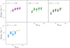	Fig. 18. Rest-frame M₁₄₅₀ binned luminosity functions of our Boötes RSQ samples (colored circles) for five non-overlapping redshift bins between 1.4 < z < 5.0. In each panel, we show as a reference the luminosity function at 1.65 < z < 2.4.
Open with DEXTER

Table 5.

Binned luminosity functions for RSQs between 1.4 < z < 5.0.

7. Results

7.1. Model-fitting

The observed evolution of the AGN luminosity function has traditionally been studied using luminosity (Boyle et al. 2000; Croom et al. 2009a; Richards et al. 2006), density (McGreer et al. 2013; Willott et al. 2010; Kashikawa et al. 2015), and even hybrid luminosity-density models (Ueda et al. 2003; Hasinger et al. 2005; Ross et al. 2013; Palanque-Delabrouille et al. 2016). These studies have found that the evolution of the luminosity function of quasars can be described by a pure luminosity evolution (PLE) model at z < 2.2 (Croom et al. 2009a), while a combined luminosity evolution and density evolution (LEDE) model can describe its evolution at z ≳ 2.2 (Croom et al. 2009a; Ross et al. 2013; Palanque-Delabrouille et al. 2016). The PLE introduces the redshift-dependence of the break magnitude using the following second-order polynomial (Croom et al. 2009a)

(12)

while the LEDE model introduces the redshift-dependence in the normalization and break magnitude using the following log-linear ansatz:

(13)

(14)

where z_p is the pivot redshift. Following previous works (e.g., Ross et al. 2013), we employ the PLE model to fit our binned luminosity function for redshift intervals z < 2.4, while at z > 2.4 we use the LEDE model with z_p = 2.4.

We use the χ² minimization to fit the luminosity function data points in each redshift bin to the corresponding models described above. Because of the relatively small area (∼9.3 deg²) of the Boötes field, there are only a few bright quasars in our sample. This implies that the bright-end slope β will be determined with high-uncertainty due to small number statistics. Therefore, we fix the bright-end slope β to the values reported by Ross et al. (2013) in their study of the quasar luminosity function using SDSS-DR9/BOSS data (Ahn et al. 2012). Additionally, we fix the parameters (k₁, k₂) and (c₁, c₂) in the PLE and LEDE models, respectively, to the values obtained by Ross et al. (2013). The parameter values from Ross et al. (2013) are chosen to match our redshift intervals. For the LEDE model, we use the parameter values corresponding to their S82 sample. Using the parameters from their DR9 sample produces similar results. Finally, the best-fit parameters and their associated uncertainties are summarized in Table 6. The corresponding best-fit model is shown with a colored line in each subpanel of Fig. 19. The models have a good agreement with the binned luminosity function.

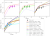Fig. 19.

Rest-frame M₁₄₅₀ binned luminosity functions of our Boötes RSQ samples (colored circles) for four non-overlapping redshift intervals between 1.4 < z < 5.0. The lines show the corresponding best-fit models in each redshift bin. The best-fitting parameters for each fit are presented in Table 6. For comparison, we show the QLFs from previous works (Cirasuolo et al. 2005; Siana et al. 2008; McGreer et al. 2009, 2018; Glikman et al. 2011; Masters et al. 2012; Ross et al. 2013; Giallongo et al. 2015; Tuccillo et al. 2015; Akiyama et al. 2018) measured over similar redshift intervals. The single-power law fits by McGreer et al. (2009) and Tuccillo et al. (2015) are plotted in the range −29 ≤ M₁₄₅₀ ≤ −26, which is the original range where they were measured.

Open with DEXTER

Table 6.

Parametric model best-fit parameters and uncertainties.

7.2. Comparison to previous works

In Fig. 19, we also compare our best-fit models with previous works. The SDSS-III/BOSS luminosity function (Ross et al. 2013) was estimated at 2.2 < z < 3.5 employing a uniform sample of 22301 quasars over an area of 2236 deg². Additionally, Ross et al. (2013) investigated the evolution of the QLF using a combination of SDSS (Richards et al. 2006), boss21+MMT and BOSS Stripe 82 datasets to over a redshift range of 0.3 < z < 4.75. Ross et al. (2013) fitted their QLF data using a PLE model at z < 2.2, while their fittings at z > 2.2 were carried out employing a LEDE model. Furthermore, we compare our results with previous surveys of faint quasars (M₁₄₅₀ ≤ −22.0) (Siana et al. 2008; Glikman et al. 2011; Giallongo et al. 2015; Masters et al. 2015; Akiyama et al. 2018; McGreer et al. 2018). The survey area of these studies ranges from 170 arcmin² (Giallongo et al. 2015) to 339.8 deg² (Akiyama et al. 2018). Finally, we also consider the results of SDSS and 2QZ (Croom et al. 2001, 2004) radio-selected samples (Cirasuolo et al. 2005; McGreer et al. 2009; Tuccillo et al. 2015) using FIRST (Becker et al. 1995). It is clear that the number density of our RSQs at all redshifts considered is lower in comparison with that of samples of optically bright and faint quasars, which are composed of both radio-detected and radio-undetected objects. Naturally, the number density of RSQs is higher than the density of SDSS/2QZ FIRST-selected samples (Cirasuolo et al. 2005; McGreer et al. 2009; Tuccillo et al. 2015), which are composed mainly of radio-loud quasars with fluxes S_1.4 GHz > 1.0 mJy. This flux limit corresponds to a LOFAR flux of S_150 MHz > 4.80 mJy, assuming a spectral index of α = −0.7. As can be seen in the bottom panel of Fig. 8, the fraction of quasars fluxes with S_150 MHz > 4.80 mJy is just 18% of the total number of RSQs in our sample. Therefore, the lower number densities presented by SDSS/2QZ FIRST-selected samples are expected.

We compare our best-fit parameters with previous studies at different redshifts to constrain the evolution of the luminosity function of RSQs. In Fig. 20, we compare the normalization constant log(Φ^*), the break magnitude , and the faint-end slope α with previous values reported for faint quasars as a function of redshift. We also plot the PLE and LEDE models by Ross et al. (2013), as well as our PLE and LEDE models. From Fig. 20, we find the following trends:

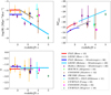Fig. 20.

Best-fit quasar luminosity function parameters as a function of redshift. Our results are indicated by purple circles, while estimates from the literature (Siana et al. 2008; Glikman et al. 2011; Masters et al. 2012; Niida et al. 2016; Akiyama et al. 2018; Yang et al. 2018; McGreer et al. 2018) are represented by the corresponding symbols in the legend box. The red and gray lines represent the PLE and LEDE models from Ross et al. (2013), and the blue and dark cyan lines our PLE (1.4 < z < 2.4) and LEDE (2.4 < z < 5.0) models listed on Table 6. For clarity, we shift vertically the PLE and LEDE models from Ross et al. (2013) by a factor of +0.1 in the third panel.

Open with DEXTER

1. Our log(Φ^*) values are lower in comparison with those of other samples of faint quasars (Siana et al. 2008; Glikman et al. 2011; Masters et al. 2012; Niida et al. 2016; Yang et al. 2018; Akiyama et al. 2018). For redshifts z < 2.4, the normalization constant within uncertainties is consistent with a PLE evolutionary trend. At z > 2.4, log(Φ^*) seems to decrease following a linear-log trend reminiscence of a LEDE evolution, and similar to that of the faint quasars.

2. The break magnitude seems to get brighter with increasing redshift, a trend that is consistent with previously estimates (Siana et al. 2008; Glikman et al. 2011; Masters et al. 2015; Niida et al. 2016).

3. The faint-end slope α does become steeper with increasing redshift with a mean value of α = −1.15 at z < 2.4, while at z > 2.4 the mean value is α = −1.26. Our α values are consistent within error bars with those reported previously by several authors (Siana et al. 2008; Glikman et al. 2011; Niida et al. 2016; Akiyama et al. 2018; Yang et al. 2018).

7.3. Density evolution of RSQs

In the last 20 years, the evolution of quasar activity has been studied in the UV/optical (Fan et al. 2001; Wolf et al. 2003; Richards et al. 2006; Fontanot et al. 2007; Bongiorno et al. 2007; Croom et al. 2009a; Glikman et al. 2011; Ross et al. 2013; Masters et al. 2015; Jiang et al. 2016; McGreer et al. 2018; Yang et al. 2018), X-ray (Hasinger et al. 2005; Silverman et al. 2005; Aird et al. 2015; Georgakakis et al. 2015; Miyaji et al. 2015), infrared (Brown et al. 2006; Siana et al. 2008; Assef et al. 2011), and radio (Vigotti et al. 2003; Carballo et al. 2006; Cirasuolo et al. 2006; McGreer et al. 2009; Tuccillo et al. 2015). Here, we study this evolution using the spatial density of quasars (Fan et al. 2001; McGreer et al. 2013; Tuccillo et al. 2015)

(15)

where Φ(M₁₄₅₀, z ) is the luminosity function of quasars, and it is integrated over all quasars more luminous than M₁₄₅₀. The integration is performed using the binned luminosity functions instead of using the best-fit luminosity functions, as it avoids uncertainties related to the model fitting and the extrapolation of the models. An upper limit of M₁₄₅₀ = −22.0 is selected for the integration as it is the lowest luminosity limit that is common between our work and other samples of faint quasars, when comparing their spatial density.

Figure 21 displays the space density of RSQs (M₁₄₅₀ ≤ −22.0) from our sample as a function of redshift, along with other faint quasar samples from the literature. Our spatial density estimates have lower values in comparison with those of other samples. However, our spatial density values show a very similar redshift evolution to that of faint quasars, and this trend continues towards z = 5.0. It is clear that a peak in quasar activity occurs around z ≈ 2.0 according to our results and the surveys carried out by Bongiorno et al. (2007) and Yang et al. (2018). This agrees with the picture provided by measurements of the luminosity function using samples of bright quasars (M₁₄₅₀ ≤ −24.0) (e.g., Richards et al. 2006; Croom et al. 2009a; Ross et al. 2013). However, the quasar samples by Akiyama et al. (2018) and Glikman et al. (2011) display space densities much higher than expected in comparison with the trend suggested by our results and other samples of faint quasars (Bongiorno et al. 2007; Masters et al. 2015; Yang et al. 2018; Siana et al. 2008; McGreer et al. 2018). These higher spatial densities could be attributed to sample contamination (Akiyama et al. 2018) or cosmic variance (Glikman et al. 2011). Finally, and as expected, our values of the space density of RSQs are significantly higher in comparison to those previously estimated for RLQs. Samples of RLQs present space density values of just a few Gpc⁻³ (e.g., Vigotti et al. 2003; Tuccillo et al. 2015). This highlights the fact that deep LOFAR observations allow us to detect the radio-emission of quasars that otherwise would be classified as radio-quiet (Retana-Montenegro & Röttgering 2018).

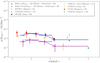Fig. 21.

Spatial density of RSQs with M₁₄₅₀ < −22 as a function of redshift compared to the space density of faint quasar samples (M₁₄₅₀ < −22) from the literature. The spatial density of RSQs is indicated by purple circles, while estimates from the literature (Bongiorno et al. 2007; Siana et al. 2008; Glikman et al. 2011; Masters et al. 2012; Akiyama et al. 2018; Yang et al. 2018; McGreer et al. 2018) are represented by the corresponding symbols in the legend box. We also plot the spatial density of RSQs scaled by a factor of 5.0 (1/0.20) (blue circles).

Open with DEXTER

Having computed the spatial density for the relevant samples of faint quasars and our RSQ sample, we calculate their normalized to z ∼ 2 spatial densities as a function of redshift. In the left panel of Fig. 22, we show the normalized spatial density of RSQs and faint quasars with M₁₄₅₀ < −22. It is clear that the space density of faint quasars and RSQs decreases rapidly with redshift. From its maximum at z ∼ 2, the space density of faint quasars (RSQs) declines between z ≃ 2 and z ≃ 3 by a factor of 1.74 ± 0.84 (1.54 ± 0.84), while it reduces further from z ≃ 2 to z ≃ 5.0 by a factor of 5.23 ± 1.41 (4.78 ± 3.61). At z ∼ 1.5, the normalized space-density ratio is 1.07 ± 0.59 (1.57 ± 1.15). Note the agreement within error bars between the evolution of the space density of RSQs and that of other faint quasar samples (Bongiorno et al. 2007; Siana et al. 2008; Masters et al. 2015; Yang et al. 2018). Considering the works by Akiyama et al. (2018) and Glikman et al. (2011), the space density of faint quasars decreases from z ≃ 2 to z ≃ 5.0 by a factor of 3.54 ± 0.87.

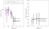Fig. 22.

Left panel: spatial densities, normalized to z ∼ 2, as a function of redshift for optically faint quasars and RSQs. Our results are indicated by fuchsia circles, while the spatial density for faint quasars is determined from results reported in the literature (Bongiorno et al. 2007; Siana et al. 2008; Glikman et al. 2011; Masters et al. 2012; Akiyama et al. 2018; Yang et al. 2018) and is denoted by green triangles. The downward triangle indicates the spatial density excluding the results by Glikman et al. (2011) and Akiyama et al. (2018), while the value denoted the downward triangle includes them. Right panel: relative fraction of RSQs with respect to the spatial density of faint quasars as a function of redshift. The ratio is calculated between overlapping redshift bins. The gray solid line indicates the mean ratio of 0.22 excluding the works by Glikman et al. (2011) and Akiyama et al. (2018), while the dashed line denotes a mean ratio of 0.18 including these works.

Open with DEXTER

Only a small fraction, less than 10%, of the quasars are classified as radio-loud (Kellermann et al. 1989; Ivezić et al. 2002; Jiang et al. 2007). However, RLQs are often associated with massive host galaxies (Shen et al. 2009; Retana-Montenegro & Röttgering 2017, and references therein), whose radio emission is produced by large and powerful radio jets (Bridle et al. 1994; Mullin et al. 2008). However, the dependency of the radio-loud fraction (RLF) of quasars on redshift and luminosity is still a matter of debate. Some authors have found that the RLF is a strong function of luminosity (e.g., Padovani 1993; La Franca et al. 1994) and redshift (e.g., Peacock et al. 1986; Miller et al. 1990; Visnovsky et al. 1992), while others have found that it does not depend significantly on either redshift or luminosity (e.g., Stern et al. 2000; Cirasuolo et al. 2003). Kratzer & Richards (2015) found that selection effects could be biasing the conclusions about the evolution of the RLF. Using the LoTSS survey (Shimwell et al. 2019), Gurkan et al. (2019) showed that quasars exhibit a wide continuum of radio properties, with no clear bimodality in the radio-loudness parameter.

In the context of this work, we compute the relative fraction of RSQs with respect to the spatial density of faint quasars as a function of redshift by dividing the spatial density of RSQs, ρ_RSQs(z), by the spatial density of faint quasars (radio-detected plus radio-undetected), ρ_QSO(z). Figure 22 displays the relative fraction of RSQs, ρ_RSQs(z)/ρ_QSO(z), as a function of redshift. The relative fraction of RSQs considering the error bars and excluding the results of Glikman et al. (2011) and Akiyama et al. (2018) is roughly independent of redshift, with a median value of 0.22 ± 0.16. This fraction is of 0.18 ± 0.14 considering the results of Glikman et al. (2011) and Akiyama et al. (2018). In Fig. 22, the spatial density of RSQs is multiplied by a factor of 5.0 (1/0.20) to compare it with the spatial density of faint quasars. With the multiplicative factor applied, the agreement between the two spatial densities is good. Moreover, it highlights the similarity in the redshift evolution of RSQs and faint quasars up to z ∼ 5. A fraction of ∼0.20 of RSQs with respect to faint quasars is relatively higher than the fractions of ∼0.10 − 0.15 of RLQs with respect to the whole quasar population previously estimated (e.g., Goldschmidt et al. 1999; Stern et al. 2000; Jiang et al. 2007). However, this is not unexpected; as previously mentioned, our deep LOFAR observations allow us to detect the radio-emission of a considerable number of quasars that otherwise would be identified as radio-quiet.

Finally, our results for the spatial density of RSQs demonstrate that the selection of quasars utilizing ML algorithms that combines optical and infrared with LOFAR observations (see Sect. 3.3.5) is very efficient and robust.

8. Discussion

In this section, we discuss several aspects related to RSQs such as: the origins of their radio-emission, the environments where these objects reside, and their location in spectroscopic parameter spaces.

8.1. The origins of radio-emission in RSQs

An important piece of information that is needed to understand the origins of the radio-emission in RSQs could come from their observed radio-morphologies. Although some of the brightest RLQs have double-lobed radio morphologies, the majority of intermediate-luminosity RLQs show core dominated radio-morphologies (de Vries et al. 2006; Lu et al. 2007; Coziol et al. 2017). Approximately, 92% of RSQs in our sample present compact radio-morphology at the resolution of the LOFAR-Boötes mosaic. A possible explanation for the origin of radio-emission in these objects lies in the interaction between outflows and the IGM, as first suggested by Stocke et al. (1992) to explain the low radio-emission in broad absorption-line quasars (BALQSOs). In this mechanism, radio-emission originates from particles accelerated on the shock fronts caused by the collision of uncollimated central outflows with the IGM of the host galaxy (Zakamska & Greene 2014; Zakamska et al. 2016). This scenario is supported by the observations of BALQSOs, as these objects have intermediate radio-luminosities and the majority present core dominated radio-morphologies (Becker et al. 2000; Liu et al. 2008; DiPompeo et al. 2011; Morabito et al. 2019), along with core-jet structures (Kunert-Bajraszewska et al. 2015) and lobes (Welling et al. 2014) in some instances. Assuming that the absorbing troughs observed in the spectra of BALQSOs are caused by uncollimated central outflows loaded into the broad emission-line region (BELR), the low numbers of BAL systems in RLQs with double-lobed radio morphology (DiPompeo et al. 2011; Pu 2013; Welling et al. 2014) can be attributed to the fact that in these quasars the central outflows form collimated jets which are physically separated from the BELR. In this scenario, the lack of radio-emission in quasars, traditionally classified as radio-quiet, can be explained considering that in a majority of cases the outflowing material is slowed down by a dense interstellar clump and the formation of shock fronts is hindered. In our LOFAR-Boötes mosaic, we detect the radio-emission of many quasars that in previous radio surveys would have remained undetected. The radio-emission in these quasars could have originated from the interaction between quasar outflows and the IGM. However, deeper optical and low-frequency radio surveys, in addition to LOFAR sub-arcsecond resolution observations (Varenius et al. 2015; Morabito et al. 2016), are needed to explore this mechanism in detail.

8.2. The environment of RSQs

A fraction of 92% of RSQs in our sample could be classified as compact steep-spectrum sources (CSS) according to their radio properties. CSS sources are usually a fraction of ∼10 − 30% in previous radio surveys (Peacock & Wall 1982; Fanti et al. 1990; O’Dea 1998), and they are characterized by their small projected linear sizes and median steep radio spectrum (α < −0.77, O’Dea 1998). The brighter RSQs in our sample have a steep spectral index distribution with a median value of α ⋍ −0.70 (Retana-Montenegro & Röttgering 2018), and only 8% of RSQs in our sample present morphologies consistent with core-jet structures.

It has been suggested that CSS may be small either because they are young and still in an early stage of their evolutionary path, eventually developing into Fanaroff-Riley type-I/II (Fanaroff & Riley 1974) radio sources (Fanti et al. 1995; Alexander 2000; Snellen et al. 2000; Collier et al. 2016), or because they are embedded in a very dense environment that frustrates the propagation of the radio jets (van Breugel et al. 1984; Fanti et al. 1986, 1989; Orienti et al. 2007). The compactness of their radio-morphologies suggests that RSQs may reside in host galaxies with a large supply of gas to fuel the early stages of quasar activity. Ultimately, these scenarios will have to be tested against high-resolution observations with submillimeter and radio interferometers that can spatially resolve the host-galaxies of RSQs and their synchrotron-dominated core-jets, respectively. These observations will, in turn, help us to shed light on the complex interplay between RSQs and their host-galaxies, and how quasar activity is triggered in these systems.

8.3. RSQs and their location in spectroscopic parameter spaces

The most striking features of Fig. 22, excluding the results by Glikman et al. (2011) and Akiyama et al. (2018) from the analysis are: (i) RSQs show evolutionary trends and declining factors that are similar to those presented by faint quasars (M₁₄₅₀ ≤ −22.0) (see Figs. 20–22), and (ii) the fact that RSQs may compose to up 22 ± 16% of the total faint quasar population, a fraction that within uncertainties is independent of redshift (see Fig. 22). Interestingly, similar decline factors in the space density of low- (Warren et al. 1994; Croom et al. 2009a; Palanque-Delabrouille et al. 2016) and high- (Schmidt et al. 1995; Kennefick et al. 1995; Palanque-Delabrouille et al. 2016) optical luminosity quasars, respectively, had been reported before. In these works, high-luminosity quasars have declining factors of ≃2 − 3 between z ≈ 2 and z ≈ 4, while low-luminosity quasars present steeper declining factors of ≃6 − 8 between the same redshift intervals. These factors are consistent with a downsizing evolutionary scenario. In this scenario, high-luminosity quasars evolve first at earlier epochs and reach their maximum space density at high-z, while low-luminosity quasars predominantly evolve at later epochs reaching their maximum space density at low-z (e.g., Hasinger et al. 2005; Silverman et al. 2005; Croom et al. 2009a). Declining factors similar to those of high-luminosity quasars had been reported for RLQs samples (Hook et al. 1998; Vigotti et al. 2003).

Since the early 2000’s there has been substantial advances in our understanding of quasars using the broad emission line properties and their correlations. Probably, the most widely used broad emission line correlations are the eigenvector 1 (E1) and C_IV parameter spaces. The E1 parameter space started as the primary eigenvector in the Principal Component Analysis performed by Boroson & Green (1992), where Fe_II and H_β emission are related to line width. The generalization of this concept led to the 4D Eigenvector 1 (4DE1) parameter space, with the addition of the properties of the C_IV and the soft X-ray photon index (Sulentic et al. 2000a,b). The 4DE1 parameter space serves as a 4D equivalent of the 2D Hertzsprung-Russell diagrams (Hertzsprung 1909; Russell 1914). This parameter space has revealed a principal sequence of quasars characterized by the Eddington ratio, and since its introduction has become an important tool for depicting the diversity of quasars and their evolutionary states (see Sulentic & Marziani 2015, and references therein). The C_IV parameter space (C_IV EW versus C_IV blueshift) has been used to study different quasar properties at high-z (e.g., Brotherton & Francis 1999; Sulentic et al. 2007; Richards et al. 2011; Kratzer & Richards 2015; Coatman et al. 2016). In the context of the 4DE1, E1, and C_IV parameter spaces, several authors (Sulentic et al. 2003, 2007; Zamfir et al. 2008; Richards et al. 2011) have determined that RLQs and RQQs are clustered at different locations in their corresponding parameter spaces (see Fig. 14 in Richards et al. 2011 and Fig. 3 in Sulentic et al. 2003). In particular, Richards et al. (2011) and Kratzer & Richards (2015) demonstrated using the E1 and C_IV spaces, which may trace the relative power of radiation line-driven accretion disk winds (Richards et al. 2011), that on average RLQs present weaker radiation line-driven winds in comparison with RQQs. These authors suggest that RLQs and RQQs are two parallel evolutionary sequences, and possibly a series of spin and merge events (Sikora et al. 2007; Sikora 2009; Schulze et al. 2017) are responsible for the triggering of radio jets, and turning RQQs into radio-loud.

Considering that RSQs present evolutionary trends similar to those of both faint quasars and bright quasars, it is possible that faint (radio and optically) RSQs could share properties of both RLQs and RQQs. Thus, RSQs would occupy intermediate locations between RQQs and RLQs in their corresponding E1, 4DE1 and C_IV parameter spaces. Future spectroscopic studies of RSQs would be a major step forward towards understanding radio-loudness.

9. Conclusions

In this work, we train three ML algorithms: RF, SVM, and Bootstrap aggregation with optical and infrared imaging to compile a sample of quasars in the 9.3 deg² Boötes field. We eliminate stellar and likely galaxy contaminants from our sample by requiring a ≥5σ detection in deep LOFAR imaging by applying a morphological criterium, respectively. The requirement of a ≥5σ LOFAR detection does not only allow us to eliminate the stellar contamination in our sample, but also to reduce the number of contaminants by two orders of magnitude. The final sample consists of 130 quasars with either spectroscopic or photometric redshifts in the range of 1.4 ≤ z ≤ 5.0. We estimate the photometric redshifts of the photometric quasars using the NW kernel regression estimator (Nadaraya 1964; Watson 1964). When comparing the predictions of this method to the spectroscopic redshifts of 1193 Boötes spectroscopic quasars, we find that 76% of the quasars have photometric redshifts that are within |δz| ≤ 0.3 of their spectroscopic redshifts. The spectral energy distributions calculated using deep photometry available for the NDWFS-Boötes field confirm the validity of the photometrically selected quasars using the ML algorithms as robust candidate quasars. We demonstrate that in cases of lack of deep and complete mid-infrared coverage needed to perform a wedge-based mid-infrared selection of AGNs, the selection of quasars using ML algorithms trained with optical and infrared photometry in combination with LOFAR data is an effective approach for obtaining samples of quasars. We compute the fraction of quasars missed due to our selection (i.e. selection function) using a library of simulated quasar spectra. The binned optical luminosity function of RSQs is computed using the 1/V_max method (Schmidt 1968) in five different redshift bins between 1.4 ≤ z ≤ 5.0. These luminosity functions are corrected for incompleteness due to the radio observations and selection method employed. The parametric fits to the binned optical luminosity function of RSQs are consistent with a PLE evolution model at z < 2.4, and a LEDE evolution at z > 2.4.

We have studied the optical luminosity function of RSQs down to faint luminosities of M₁₄₅₀ = −22. Previous studies were mostly limited to bright RLQs with luminosities M₁₄₅₀ = −26 (Cirasuolo et al. 2005; Carballo et al. 2006; McGreer et al. 2009; Tuccillo et al. 2015). We find evidence that suggests that the faint-end slope α is becoming steeper with increasing redshift, as found by previous measurements of the luminosity function of faint quasars (Glikman et al. 2011; Giallongo et al. 2015). Our mean values of the faint-end slope are α = −1.15 at z < 2.4, while at z > 2.4 the mean value is α = −1.26. We calculate the space density of RSQs over 1.4 ≤ z ≤ 5.0 and find an evolutionary trend below and above the peak of their space density that is comparable to that of faint quasars. By comparing the spatial density of RSQs with that of faint quasars at similar redshifts, we find that RSQs may compose to up 22 ± 16% of the total faint quasar population. This fraction, within uncertainties, seems to remain constant with redshift. We argue that considering the similarities in evolutionary trends and declining factors between RSQs and faint quasars, the fainter (optically and radio) RSQs may have properties of both RLQs and RQQs. Finally, we discuss several aspects of RSQs such as: the origins of their radio emission, the environments where these objects reside, and their location in E1, 4DE1 and C_IV parameter spaces.

Our work demonstrates the feasibility of studying the evolution of RSQs using samples of quasars compiled with ML algorithms trained with optical and infrared photometry combined with LOFAR data. Future studies of the luminosity function of RSQs will benefit from the advent of the new generation of wide-field radio (LOTSS: Röttgering et al. 2011; Shimwell et al. 2017, 2019; EMU: Norris et al. 2011), optical (LSST: Tyson 2002; LSST Science Collaboration 2009; DES: Flaugher 2005), infrared (WFIRST: Spergel et al. 2013; Euclid: Laureijs et al. 2011), and spectroscopic surveys (EBOSS: Dawson et al. 2016; DESI: DESI Collaboration 2016).

¹

https://irsa.ipac.caltech.edu/data/COSMOS/gator_docs/scosmos_irac_colDescriptions.html

²

http://skyserver.sdss.org/CasJobs/

³

https://mastweb.stsci.edu/ps1casjobs/

⁴

http://wise2.ipac.caltech.edu/docs/release/allsky/expsup/

⁵

https://www.sdss.org/dr14/algorithms/magnitudes/

⁶

http://quasars.org/

⁷

https://scikit-learn.org

⁸

https://ned.ipac.caltech.edu/

⁹

https://www.sdss.org/dr14/algorithms/classify/

¹⁰

https://www.sdss.org/dr14/algorithms/magnitudes/

Acknowledgments

ERM acknowledges financial support from NWO Top project, No. 614.001.006. HR acknowledges support from the ERC Advanced Investigator program NewClusters 321271. ERM acknowledges the valuable suggestions and comments from H. Andernach. Moreover, we would like to thank the referee for valuable suggestions on the manuscript. LOFAR, the Low Frequency Array designed and constructed by ASTRON, has facilities in several countries, that are owned by various parties (each with their own funding sources), and that are collectively operated by the International LOFAR Telescope (ILT) foundation under a joint scientific policy. The Open University is incorporated by Royal Charter (RC 000391), an exempt charity in England & Wales and a charity registered in Scotland (SC 038302). The Open University is authorized and regulated by the Financial Conduct Authority. Funding for the Sloan Digital Sky Survey IV has been provided by the Alfred P. Sloan Foundation, the US Department of Energy Office of Science, and the Participating Institutions. SDSS- IV acknowledges support and resources from the Center for High-Performance Computing at the University of Utah. The SDSS web site is www.sdss.org. SDSS-IV is managed by the Astrophysical Research Consortium for the Participating Institutions of the SDSS Collaboration including the Brazilian Participation Group, the Carnegie Institution for Science, Carnegie Mellon University, the Chilean Participation Group, the French Participation Group, Harvard-Smithsonian Center for Astrophysics, Instituto de Astrofísica de Canarias, The Johns Hopkins University, Kavli Institute for the Physics and Mathematics of the Universe (IPMU)/University of Tokyo, Lawrence Berkeley National Laboratory, Leibniz Institut für Astrophysik Potsdam (AIP), Max-Planck-Institut für Astronomie (MPIA Heidelberg), Max-Planck-Institut für Astrophysik (MPA Garching), Max-Planck-Institut für Extraterrestrische Physik (MPE), National Astronomical Observatory of China, New Mexico State University, New York University, University of Notre Dame, Observatório Nacional/MCTI, The Ohio State University, Pennsylvania State University, Shanghai Astronomical Observatory, United Kingdom Participation Group, Universidad Nacional Autónoma de México, University of Arizona, University of Colorado Boulder, University of Oxford, University of Portsmouth, University of Utah, University of Virginia, University of Washington, University of Wisconsin, Vanderbilt University, and Yale University. The Pan-STARRS1 Surveys (PS1) have been made possible through contributions of the Institute for Astronomy, the University of Hawaii, the Pan-STARRS Project Office, the Max-Planck Society and its participating institutes, the Max Planck Institute for Astronomy, Heidelberg and the Max Planck Institute for Extraterrestrial Physics, Garching, The Johns Hopkins University, Durham University, the University of Edinburgh, Queen’s University Belfast, the Harvard-Smithsonian Center for Astrophysics, the Las Cumbres Observatory Global Telescope Network Incorporated, the National Central University of Taiwan, the Space Telescope Science Institute, the National Aeronautics and Space Administration under Grant No. NNX08AR22G issued through the Planetary Science Division of the NASA Science Mission Directorate, the National Science Foundation under Grant No. AST-1238877, the University of Maryland, and Eotvos Lorand University (ELTE). This publication makes use of data products from the Wide-field Infrared Survey Explorer, which is a joint project of the University of California, Los Angeles, and the Jet Propulsion Laboratory/California Institute of Technology, funded by the National Aeronautics and Space Administration.

References

Abolfathi, B., Aguado, D. S., Aguilar, G., et al. 2018, ApJS, 235, 42 [NASA ADS] [CrossRef] [Google Scholar]
Ahn, C. P., Alexandroff, R., Allende Prieto, C., et al. 2012, ApJS, 203, 21 [NASA ADS] [CrossRef] [Google Scholar]
Aird, J., Coil, A. L., Georgakakis, A., et al. 2015, MNRAS, 451, 1892 [NASA ADS] [CrossRef] [Google Scholar]
Akiyama, M., He, W., Ikeda, H., et al. 2018, PASJ, 70, S34 [NASA ADS] [CrossRef] [Google Scholar]
Alexander, P. 2000, MNRAS, 319, 8 [NASA ADS] [CrossRef] [Google Scholar]
Altman, N. S. 1992, Am. Stat., 46, 175 [Google Scholar]
Ashby, M. L. N., Stern, D., Brodwin, M., et al. 2009, ApJ, 701, 428 [NASA ADS] [CrossRef] [Google Scholar]
Assef, R. J., Kochanek, C. S., Ashby, M. L. N., et al. 2011, ApJ, 728, 56 [NASA ADS] [CrossRef] [Google Scholar]
Bañados, E., Venemans, B. P., Morganson, E., et al. 2015, ApJ, 804, 118 [NASA ADS] [CrossRef] [Google Scholar]
Baldwin, J. A. 1977, ApJ, 214, 679 [NASA ADS] [CrossRef] [Google Scholar]
Becker, R. H., White, R. L., & Helfand, D. J. 1995, ApJ, 450, 559 [NASA ADS] [CrossRef] [Google Scholar]
Becker, R. H., White, R. L., Gregg, M. D., et al. 2000, ApJ, 538, 72 [NASA ADS] [CrossRef] [Google Scholar]
Bershady, M. A., Charlton, J. C., & Geoffroy, J. M. 1999, ApJ, 518, 103 [NASA ADS] [CrossRef] [Google Scholar]
Bertin, E., & Arnouts, S. 1996, A&AS, 117, 393 [NASA ADS] [CrossRef] [EDP Sciences] [Google Scholar]
Bian, F., Fan, X., Jiang, L., et al. 2013, ApJ, 774, 28 [NASA ADS] [CrossRef] [Google Scholar]
Bongiorno, A., Zamorani, G., Gavignaud, I., et al. 2007, A&A, 472, 443 [NASA ADS] [CrossRef] [EDP Sciences] [Google Scholar]
Bonzini, M., Padovani, P., Mainieri, V., et al. 2013, MNRAS, 436, 3759 [NASA ADS] [CrossRef] [Google Scholar]
Boroson, T. A., & Green, R. F. 1992, ApJS, 80, 109 [NASA ADS] [CrossRef] [Google Scholar]
Bovy, J., Hennawi, J. F., Hogg, D. W., et al. 2011, ApJ, 729, 141 [NASA ADS] [CrossRef] [Google Scholar]
Boyle, B. J., Shanks, T., Croom, S. M., et al. 2000, MNRAS, 317, 1014 [NASA ADS] [CrossRef] [Google Scholar]
Brammer, G. B., van Dokkum, P. G., & Coppi, P. 2008, ApJ, 686, 1503 [NASA ADS] [CrossRef] [Google Scholar]
Breiman, L. 1996, Mach. Learn., 24, 123 [Google Scholar]
Breiman, L. 2001, Mach. Learn., 45, 5 [CrossRef] [Google Scholar]
Bridle, A. H., Hough, D. H., Lonsdale, C. J., Burns, J. O., & Laing, R. A. 1994, AJ, 108, 766 [NASA ADS] [CrossRef] [Google Scholar]
Brotherton, M. S., & Francis, P. J. 1999, in Quasars and Cosmology, eds. G. Ferland, & J. Baldwin, ASP Conf. Ser., 162, 395 [NASA ADS] [Google Scholar]
Brown, M. J. I., Brand, K., Dey, A., et al. 2006, ApJ, 638, 88 [NASA ADS] [CrossRef] [Google Scholar]
Brown, M. J. I., Dey, A., Jannuzi, B. T., et al. 2007, ApJ, 654, 858 [NASA ADS] [CrossRef] [Google Scholar]
Calzetti, D., Armus, L., Bohlin, R. C., et al. 2000, ApJ, 533, 682 [NASA ADS] [CrossRef] [Google Scholar]
Campbell, J., Lo, A., & MacKinlay, A. 2012, The Econometrics of Financial Markets (Princeton: Princeton University Press) [CrossRef] [Google Scholar]
Carballo, R., González-Serrano, J. I., Montenegro-Montes, F. M., et al. 2006, MNRAS, 370, 1034 [NASA ADS] [Google Scholar]
Carrasco, D., Barrientos, L. F., Pichara, K., et al. 2015, A&A, 584, A44 [NASA ADS] [CrossRef] [EDP Sciences] [Google Scholar]
Chabrier, G., Baraffe, I., Allard, F., & Hauschildt, P. 2000, ApJ, 542, 464 [NASA ADS] [CrossRef] [Google Scholar]
Chambers, K. C., Magnier, E. A., Metcalfe, N., et al. 2016, ArXiv e-prints [arXiv:1612.05560] [Google Scholar]
Chen, T., & Guestrin, C. 2016, ArXiv e-prints [arXiv:1603.02754] [Google Scholar]
Cirasuolo, M., Magliocchetti, M., Celotti, A., & Danese, L. 2003, MNRAS, 341, 993 [NASA ADS] [CrossRef] [Google Scholar]
Cirasuolo, M., Magliocchetti, M., & Celotti, A. 2005, MNRAS, 357, 1267 [NASA ADS] [CrossRef] [Google Scholar]
Cirasuolo, M., Magliocchetti, M., Gentile, G., et al. 2006, MNRAS, 371, 695 [NASA ADS] [CrossRef] [Google Scholar]
Coatman, L., Hewett, P. C., Banerji, M., & Richards, G. T. 2016, MNRAS, 461, 647 [NASA ADS] [CrossRef] [Google Scholar]
Collier, J. D., Norris, R. P., Filipović, M. D., & Tothill, N. F. H. 2016, Astron. Nachr., 337, 36 [NASA ADS] [CrossRef] [Google Scholar]
Condon, J. J., Kellermann, K. I., Kimball, A. E., Ivezić, Ž., & Perley, R. A. 2013, ApJ, 768, 37 [NASA ADS] [CrossRef] [Google Scholar]
Cool, R. J. 2007, ApJS, 169, 21 [NASA ADS] [CrossRef] [Google Scholar]
Cool, R. J., Kochanek, C. S., Eisenstein, D. J., et al. 2006, AJ, 132, 823 [NASA ADS] [CrossRef] [Google Scholar]
Cortes, C., & Vapnik, V. 1995, Mach. Learn., 20, 273 [Google Scholar]
Coziol, R., Andernach, H., Torres-Papaqui, J. P., Ortega-Minakata, R. A., & Moreno del Rio, F. 2017, MNRAS, 466, 921 [NASA ADS] [CrossRef] [Google Scholar]
Cristiani, S., & Vio, R. 1990, A&A, 227, 385 [NASA ADS] [Google Scholar]
Croom, S. M., Smith, R. J., Boyle, B. J., et al. 2001, MNRAS, 322, L29 [NASA ADS] [CrossRef] [Google Scholar]
Croom, S. M., Smith, R. J., Boyle, B. J., et al. 2004, MNRAS, 349, 1397 [NASA ADS] [CrossRef] [Google Scholar]
Croom, S. M., Richards, G. T., Shanks, T., et al. 2009a, MNRAS, 399, 1755 [NASA ADS] [CrossRef] [Google Scholar]
Croom, S. M., Richards, G. T., Shanks, T., et al. 2009b, MNRAS, 392, 19 [NASA ADS] [CrossRef] [Google Scholar]
Cutri, R. M. 2013, VizieR Online Data Catalog: II/328 [Google Scholar]
Czerny, B., Li, J., Loska, Z., & Szczerba, R. 2004, MNRAS, 348, L54 [NASA ADS] [CrossRef] [Google Scholar]
Dawson, K. S., Kneib, J.-P., Percival, W. J., et al. 2016, AJ, 151, 44 [NASA ADS] [CrossRef] [Google Scholar]
DESI Collaboration (Aghamousa, A., et al.) 2016, ArXiv e-prints [arXiv:1611.00036] [Google Scholar]
de Vries, W. H., Morganti, R., Röttgering, H. J. A., et al. 2002, AJ, 123, 1784 [NASA ADS] [CrossRef] [Google Scholar]
de Vries, W. H., Becker, R. H., & White, R. L. 2006, AJ, 131, 666 [NASA ADS] [CrossRef] [Google Scholar]
DiPompeo, M. A., Brotherton, M. S., De Breuck, C., & Laurent-Muehleisen, S. 2011, ApJ, 743, 71 [NASA ADS] [CrossRef] [Google Scholar]
Donley, J. L., Koekemoer, A. M., Brusa, M., et al. 2012, ApJ, 748, 142 [NASA ADS] [CrossRef] [Google Scholar]
Fan, X. 1999, AJ, 117, 2528 [NASA ADS] [CrossRef] [Google Scholar]
Fan, X., Narayanan, V. K., Lupton, R. H., et al. 2001, AJ, 122, 2833 [NASA ADS] [CrossRef] [Google Scholar]
Fanaroff, B. L., & Riley, J. M. 1974, MNRAS, 167, 31P [NASA ADS] [CrossRef] [Google Scholar]
Fanti, C., Fanti, R., Schilizzi, R. T., Spencer, R. E., & van Breugel, W. J. M. 1986, A&A, 170, 10 [NASA ADS] [Google Scholar]
Fanti, C., Fanti, R., Parma, P., et al. 1989, A&A, 217, 44 [NASA ADS] [Google Scholar]
Fanti, R., Fanti, C., Schilizzi, R. T., et al. 1990, A&A, 231, 333 [NASA ADS] [Google Scholar]
Fanti, C., Fanti, R., Dallacasa, D., et al. 1995, A&A, 302, 317 [NASA ADS] [Google Scholar]
Flaugher, B. 2005, Int. J. Mod. Phys. A, 20, 3121 [NASA ADS] [CrossRef] [Google Scholar]
Flesch, E. W. 2015, PASA, 32, e010 [NASA ADS] [CrossRef] [Google Scholar]
Fontanot, F., Cristiani, S., Monaco, P., et al. 2007, A&A, 461, 39 [NASA ADS] [CrossRef] [EDP Sciences] [Google Scholar]
Fukugita, M., Ichikawa, T., Gunn, J. E., et al. 1996, AJ, 111, 1748 [NASA ADS] [CrossRef] [Google Scholar]
Gao, D., Zhang, Y.-X., & Zhao, Y.-H. 2008, MNRAS, 386, 1417 [NASA ADS] [CrossRef] [Google Scholar]
Gavignaud, I., Bongiorno, A., Paltani, S., et al. 2006, A&A, 457, 79 [NASA ADS] [CrossRef] [EDP Sciences] [Google Scholar]
Gehrels, N. 1986, ApJ, 303, 336 [NASA ADS] [CrossRef] [Google Scholar]
Georgakakis, A., Aird, J., Buchner, J., et al. 2015, MNRAS, 453, 1946 [NASA ADS] [CrossRef] [Google Scholar]
Giallongo, E., Grazian, A., Fiore, F., et al. 2015, A&A, 578, A83 [NASA ADS] [CrossRef] [EDP Sciences] [Google Scholar]
Giallongo, E., Grazian, A., Fiore, F., et al. 2019, ApJ, 884, 19 [NASA ADS] [CrossRef] [Google Scholar]
Glikman, E., Djorgovski, S. G., Stern, D., et al. 2011, ApJ, 728, L26 [NASA ADS] [CrossRef] [Google Scholar]
Goldschmidt, P., Kukula, M. J., Miller, L., & Dunlop, J. S. 1999, ApJ, 511, 612 [NASA ADS] [CrossRef] [Google Scholar]
Gunn, J. E., Siegmund, W. A., Mannery, E. J., et al. 2006, AJ, 131, 2332 [NASA ADS] [CrossRef] [Google Scholar]
Gurkan, G., Hardcastle, M. J., Best, P. N., et al. 2019, A&A, 622, A11 [NASA ADS] [CrossRef] [EDP Sciences] [Google Scholar]
Haardt, F., & Madau, P. 2012, ApJ, 746, 125 [NASA ADS] [CrossRef] [Google Scholar]
Härdle, W. 1990, Applied Nonparametric Regression, Econometric Society Monographs (Cambridge: Cambridge University Press) [CrossRef] [Google Scholar]
Hasinger, G., Miyaji, T., & Schmidt, M. 2005, A&A, 441, 417 [NASA ADS] [CrossRef] [EDP Sciences] [Google Scholar]
Hatziminaoglou, E., Mathez, G., & Pelló, R. 2000, A&A, 359, 9 [NASA ADS] [Google Scholar]
Herrera Ruiz, N., Middelberg, E., Norris, R. P., & Maini, A. 2016, A&A, 589, L2 [NASA ADS] [CrossRef] [EDP Sciences] [Google Scholar]
Hertzsprung, E. 1909, Astron. Nachr., 179, 373 [NASA ADS] [CrossRef] [Google Scholar]
Hodapp, K. W., Siegmund, W. A., Kaiser, N., et al. 2004, in Ground-based Telescopes, eds. J. Oschmann, & M. Jacobus, SPIE Conf. Ser., 5489, 667 [NASA ADS] [CrossRef] [Google Scholar]
Hook, I. M., Shaver, P. A., & McMahon, R. G. 1998, in The Young Universe: Galaxy Formation and Evolution at Intermediate and High Redshift, eds. S. D’Odorico, A. Fontana, & E. Giallongo, ASP Conf. Ser., 146, 17 [NASA ADS] [Google Scholar]
Hook, I. M., McMahon, R. G., Shaver, P. A., & Snellen, I. A. G. 2002, A&A, 391, 509 [NASA ADS] [CrossRef] [EDP Sciences] [Google Scholar]
Ilbert, O., Arnouts, S., McCracken, H. J., et al. 2006, A&A, 457, 841 [NASA ADS] [CrossRef] [EDP Sciences] [Google Scholar]
Ivezić, Ž., Menou, K., Knapp, G. R., et al. 2002, AJ, 124, 2364 [NASA ADS] [CrossRef] [Google Scholar]
Ivezić, Ž., Brandt, W. N., Fan, X., et al. 2014, in Multiwavelength AGN Surveys and Studies, eds. A. M. Mickaelian, & D. B. Sanders, IAU Symp., 304, 11 [NASA ADS] [Google Scholar]
Ivezić, Ž., Kahn, S. M., Tyson, J. A., et al. 2019, ApJ, 873, 111 [NASA ADS] [CrossRef] [Google Scholar]
Jannuzi, B. T., & Dey, A. 1999, in Photometric Redshifts and the Detection of High Redshift Galaxies, eds. R. Weymann, L. Storrie-Lombardi, M. Sawicki, & R. Brunner, ASP Conf. Ser., 191, 111 [NASA ADS] [Google Scholar]
Jannuzi, B., Weiner, B., Block, M., et al. 2010, in Amer. Astron. Soc. Meet. Abstr., #215, BAAS, 42, 513 [Google Scholar]
Jiang, L., Fan, X., Ivezić, Ž., et al. 2007, ApJ, 656, 680 [NASA ADS] [CrossRef] [Google Scholar]
Jiang, L., McGreer, I. D., Fan, X., et al. 2016, ApJ, 833, 222 [NASA ADS] [CrossRef] [Google Scholar]
Jin, X., Zhang, Y., Zhang, J., et al. 2019, MNRAS, 485, 4539 [NASA ADS] [CrossRef] [Google Scholar]
Kashikawa, N., Ishizaki, Y., Willott, C. J., et al. 2015, ApJ, 798, 28 [NASA ADS] [CrossRef] [Google Scholar]
Kellermann, K. I., Sramek, R., Schmidt, M., Shaffer, D. B., & Green, R. 1989, AJ, 98, 1195 [NASA ADS] [CrossRef] [Google Scholar]
Kennefick, J. D., Djorgovski, S. G., & de Carvalho, R. R. 1995, AJ, 110, 2553 [NASA ADS] [CrossRef] [Google Scholar]
Kenter, A., Murray, S. S., Forman, W. R., et al. 2005, ApJS, 161, 9 [NASA ADS] [CrossRef] [Google Scholar]
Kimball, A. E., Knapp, G. R., Ivezić, Ž., et al. 2009, ApJ, 701, 535 [NASA ADS] [CrossRef] [Google Scholar]
Kimball, A. E., Kellermann, K. I., Condon, J. J., Ivezić, Ž., & Perley, R. A. 2011, ApJ, 739, L29 [NASA ADS] [CrossRef] [Google Scholar]
Kirkpatrick, J. A., Schlegel, D. J., Ross, N. P., et al. 2011, ApJ, 743, 125 [NASA ADS] [CrossRef] [Google Scholar]
Kochanek, C. S., Eisenstein, D. J., Cool, R. J., et al. 2012, ApJS, 200, 8 [NASA ADS] [CrossRef] [Google Scholar]
Kratzer, R. M., & Richards, G. T. 2015, AJ, 149, 61 [NASA ADS] [CrossRef] [Google Scholar]
Kunert-Bajraszewska, M., Cegłowski, M., Katarzyński, K., & Roskowiński, C. 2015, A&A, 579, A109 [NASA ADS] [CrossRef] [EDP Sciences] [Google Scholar]
Lacy, M., Wilson, G., Masci, F., et al. 2005, ApJS, 161, 41 [NASA ADS] [CrossRef] [Google Scholar]
Lacy, M., Petric, A. O., Sajina, A., et al. 2007, AJ, 133, 186 [NASA ADS] [CrossRef] [Google Scholar]
La Franca, F., Gregorini, L., Cristiani, S., de Ruiter, H., & Owen, F. 1994, AJ, 108, 1548 [NASA ADS] [CrossRef] [Google Scholar]
Laureijs, R., Amiaux, J., Arduini, S., et al. 2011, ArXiv e-prints [arXiv:1110.3193] [Google Scholar]
Le Fèvre, O., Cassata, P., Cucciati, O., et al. 2013, A&A, 559, A14 [NASA ADS] [CrossRef] [EDP Sciences] [Google Scholar]
Li, Q., & Racine, J. 2011, Nonparametric Econometrics: Theory and Practice (Princeton: Princeton University Press) [Google Scholar]
Liu, Y., Jiang, D. R., Wang, T. G., & Xie, F. G. 2008, MNRAS, 391, 246 [NASA ADS] [CrossRef] [Google Scholar]
Lonsdale, C. J., Smith, H. E., Rowan-Robinson, M., et al. 2003, PASP, 115, 897 [NASA ADS] [CrossRef] [Google Scholar]
LSST Science Collaboration (Abell, P. A., et al.) 2009, ArXiv e-prints [arXiv:0912.0201] [Google Scholar]
Lu, Y., Wang, T., Zhou, H., & Wu, J. 2007, AJ, 133, 1615 [NASA ADS] [CrossRef] [Google Scholar]
Lupton, R. H., Gunn, J. E., & Szalay, A. S. 1999, AJ, 118, 1406 [NASA ADS] [CrossRef] [Google Scholar]
Maddox, N., Hewett, P. C., Péroux, C., Nestor, D. B., & Wisotzki, L. 2012, MNRAS, 424, 2876 [NASA ADS] [CrossRef] [Google Scholar]
Magnier, E. A., Sweeney, W. E., Chambers, K. C., et al. 2016, ArXiv e-prints [arXiv:1612.05244] [Google Scholar]
Martin, D. C., Fanson, J., Schiminovich, D., et al. 2005, ApJ, 619, L1 [NASA ADS] [CrossRef] [Google Scholar]
Masters, D., Capak, P., Salvato, M., et al. 2012, ApJ, 755, 169 [NASA ADS] [CrossRef] [Google Scholar]
Masters, D., Capak, P., Stern, D., et al. 2015, ApJ, 813, 53 [NASA ADS] [CrossRef] [Google Scholar]
Mauduit, J. C., Lacy, M., Farrah, D., et al. 2012, PASP, 124, 1135 [NASA ADS] [CrossRef] [Google Scholar]
McGreer, I. D., Becker, R. H., Helfand, D. J., & White, R. L. 2006, ApJ, 652, 157 [NASA ADS] [CrossRef] [Google Scholar]
McGreer, I. D., Helfand, D. J., & White, R. L. 2009, AJ, 138, 1925 [NASA ADS] [CrossRef] [Google Scholar]
McGreer, I. D., Jiang, L., Fan, X., et al. 2013, ApJ, 768, 105 [NASA ADS] [CrossRef] [Google Scholar]
McGreer, I. D., Fan, X., Jiang, L., & Cai, Z. 2018, AJ, 155, 131 [NASA ADS] [CrossRef] [Google Scholar]
Meisner, A. M., Lang, D., & Schlegel, D. J. 2017, AJ, 154, 161 [NASA ADS] [CrossRef] [Google Scholar]
Messias, H., Afonso, J., Salvato, M., Mobasher, B., & Hopkins, A. M. 2012, ApJ, 754, 120 [NASA ADS] [CrossRef] [Google Scholar]
Miller, L., Peacock, J. A., & Mead, A. R. G. 1990, MNRAS, 244, 207 [NASA ADS] [Google Scholar]
Miyaji, T., Hasinger, G., Salvato, M., et al. 2015, ApJ, 804, 104 [NASA ADS] [CrossRef] [Google Scholar]
Møller, P., & Jakobsen, P. 1990, A&A, 228, 299 [NASA ADS] [Google Scholar]
Morabito, L. K., Deller, A. T., Röttgering, H., et al. 2016, MNRAS, 461, 2676 [NASA ADS] [CrossRef] [Google Scholar]
Morabito, L. K., Matthews, J. H., Best, P. N., et al. 2019, A&A, 622, A15 [NASA ADS] [CrossRef] [EDP Sciences] [Google Scholar]
Mullin, L. M., Riley, J. M., & Hardcastle, M. J. 2008, MNRAS, 390, 595 [NASA ADS] [CrossRef] [Google Scholar]
Myers, A. D., Palanque-Delabrouille, N., Prakash, A., et al. 2015, ApJS, 221, 27 [NASA ADS] [CrossRef] [Google Scholar]
Nadaraya, E. 1964, Theory Probab. Appl., 9, 141 [CrossRef] [Google Scholar]
Nakoneczny, S., Bilicki, M., Solarz, A., et al. 2019, A&A, 624, A13 [NASA ADS] [CrossRef] [EDP Sciences] [Google Scholar]
Niida, M., Nagao, T., Ikeda, H., et al. 2016, ApJ, 832, 208 [NASA ADS] [CrossRef] [Google Scholar]
Norris, R. P. 2017, Nat. Astron., 1, 671 [NASA ADS] [CrossRef] [Google Scholar]
Norris, R. P., Hopkins, A. M., Afonso, J., et al. 2011, PASA, 28, 215 [NASA ADS] [CrossRef] [Google Scholar]
O’Dea, C. P. 1998, PASP, 110, 493 [NASA ADS] [CrossRef] [Google Scholar]
Oke, J. B., & Gunn, J. E. 1983, ApJ, 266, 713 [NASA ADS] [CrossRef] [Google Scholar]
Orienti, M., Dallacasa, D., & Stanghellini, C. 2007, A&A, 461, 923 [NASA ADS] [CrossRef] [EDP Sciences] [Google Scholar]
Padovani, P. 1993, MNRAS, 263, 461 [NASA ADS] [Google Scholar]
Padovani, P., Miller, N., Kellermann, K. I., et al. 2011, ApJ, 740, 20 [NASA ADS] [CrossRef] [Google Scholar]
Palanque-Delabrouille, N., Magneville, C., Yèche, C., et al. 2016, A&A, 587, A41 [NASA ADS] [CrossRef] [EDP Sciences] [Google Scholar]
Papovich, C., Cool, R., Eisenstein, D., et al. 2006, AJ, 132, 231 [NASA ADS] [CrossRef] [Google Scholar]
Papovich, C., Shipley, H. V., Mehrtens, N., et al. 2016, ApJS, 224, 28 [NASA ADS] [CrossRef] [Google Scholar]
Pâris, I., Petitjean, P., Aubourg, É., et al. 2018, A&A, 613, A51 [NASA ADS] [CrossRef] [EDP Sciences] [Google Scholar]
Pasquet, J., Bertin, E., Treyer, M., Arnouts, S., & Fouchez, D. 2019, A&A, 621, A26 [NASA ADS] [CrossRef] [EDP Sciences] [Google Scholar]
Pasquet-Itam, J., & Pasquet, J. 2018, A&A, 611, A97 [NASA ADS] [CrossRef] [EDP Sciences] [Google Scholar]
Peacock, J. A., & Wall, J. V. 1982, MNRAS, 198, 843 [NASA ADS] [Google Scholar]
Peacock, J. A., Miller, L., & Longair, M. S. 1986, MNRAS, 218, 265 [NASA ADS] [Google Scholar]
Pei, Y. C. 1992, ApJ, 395, 130 [NASA ADS] [CrossRef] [Google Scholar]
Pei, Y. C. 1995, ApJ, 438, 623 [NASA ADS] [CrossRef] [Google Scholar]
Peng, N., Zhang, Y., Zhao, Y., & Wu, X.-B. 2012, MNRAS, 425, 2599 [NASA ADS] [CrossRef] [Google Scholar]
Peters, C. M., Richards, G. T., Myers, A. D., et al. 2015, ApJ, 811, 95 [NASA ADS] [CrossRef] [Google Scholar]
Prandoni, I., de Ruiter, H. R., Ricci, R., et al. 2010, A&A, 510, A42 [NASA ADS] [CrossRef] [EDP Sciences] [Google Scholar]
Pu, X. 2013, Ap&SS, 345, 355 [NASA ADS] [CrossRef] [Google Scholar]
Qiu, P. 2013, Introduction to Statistical Process Control, Chapman & Hall/CRC Texts in Statistical Science (CRC Press) [CrossRef] [Google Scholar]
Retana-Montenegro, E., & Röttgering, H. J. A. 2017, A&A, 600, A97 [NASA ADS] [CrossRef] [EDP Sciences] [Google Scholar]
Retana-Montenegro, E., & Röttgering, H. 2018, Front. Astron. Space Sci., 5, 5 [NASA ADS] [CrossRef] [Google Scholar]
Retana-Montenegro, E., Röttgering, H. J. A., Shimwell, T. W., et al. 2018, A&A, 620, A74 [NASA ADS] [CrossRef] [EDP Sciences] [Google Scholar]
Richards, G. T., Weinstein, M. A., Schneider, D. P., et al. 2001, AJ, 122, 1151 [NASA ADS] [CrossRef] [Google Scholar]
Richards, G. T., Fan, X., Newberg, H. J., et al. 2002, AJ, 123, 2945 [NASA ADS] [CrossRef] [Google Scholar]
Richards, G. T., Strauss, M. A., Fan, X., et al. 2006, AJ, 131, 2766 [NASA ADS] [CrossRef] [Google Scholar]
Richards, G. T., Myers, A. D., Gray, A. G., et al. 2009, ApJS, 180, 67 [NASA ADS] [CrossRef] [Google Scholar]
Richards, G. T., Kruczek, N. E., Gallagher, S. C., et al. 2011, AJ, 141, 167 [NASA ADS] [CrossRef] [Google Scholar]
Richards, G. T., Myers, A. D., Peters, C. M., et al. 2015, ApJS, 219, 39 [NASA ADS] [CrossRef] [Google Scholar]
Ross, N. P., McGreer, I. D., White, M., et al. 2013, ApJ, 773, 14 [NASA ADS] [CrossRef] [Google Scholar]
Röttgering, H., Afonso, J., Barthel, P., et al. 2011, JApA, 32, 557 [NASA ADS] [CrossRef] [Google Scholar]
Russell, H. N. 1914, Pop. Astron., 22, 275 [NASA ADS] [Google Scholar]
Salvato, M., Hasinger, G., Ilbert, O., et al. 2009, ApJ, 690, 1250 [NASA ADS] [CrossRef] [Google Scholar]
Sanders, D. B., Salvato, M., Aussel, H., et al. 2007, ApJS, 172, 86 [NASA ADS] [CrossRef] [Google Scholar]
Schindler, J.-T., Fan, X., McGreer, I. D., et al. 2017, ApJ, 851, 13 [NASA ADS] [CrossRef] [Google Scholar]
Schlafly, E. F., & Finkbeiner, D. P. 2011, ApJ, 737, 103 [NASA ADS] [CrossRef] [Google Scholar]
Schmidt, M. 1968, ApJ, 151, 393 [NASA ADS] [CrossRef] [Google Scholar]
Schmidt, M., Schneider, D. P., & Gunn, J. E. 1995, AJ, 110, 68 [NASA ADS] [CrossRef] [Google Scholar]
Schneider, D. P., Richards, G. T., Hall, P. B., et al. 2010, AJ, 139, 2360 [NASA ADS] [CrossRef] [Google Scholar]
Schulze, A., Done, C., Lu, Y., Zhang, F., & Inoue, Y. 2017, ApJ, 849, 4 [NASA ADS] [CrossRef] [Google Scholar]
Scranton, R., Johnston, D., Dodelson, S., et al. 2002, ApJ, 579, 48 [NASA ADS] [CrossRef] [Google Scholar]
Shaver, P. A., Wall, J. V., Kellermann, K. I., Jackson, C. A., & Hawkins, M. R. S. 1996, Nature, 384, 439 [NASA ADS] [CrossRef] [Google Scholar]
Shen, Y., Strauss, M. A., Ross, N. P., et al. 2009, ApJ, 697, 1656 [NASA ADS] [CrossRef] [Google Scholar]
Shimwell, T. W., Röttgering, H. J. A., Best, P. N., et al. 2017, A&A, 598, A104 [NASA ADS] [CrossRef] [EDP Sciences] [Google Scholar]
Shimwell, T. W., Tasse, C., Hardcastle, M. J., et al. 2019, A&A, 622, A1 [NASA ADS] [CrossRef] [EDP Sciences] [Google Scholar]
Siana, B., Polletta, M. D. C., Smith, H. E., et al. 2008, ApJ, 675, 49 [NASA ADS] [CrossRef] [Google Scholar]
Sikora, M. 2009, Astron. Nachr., 330, 291 [NASA ADS] [CrossRef] [Google Scholar]
Sikora, M., Stawarz, Ł., & Lasota, J.-P. 2007, ApJ, 658, 815 [NASA ADS] [CrossRef] [Google Scholar]
Silverman, J. D., Green, P. J., Barkhouse, W. A., et al. 2005, ApJ, 624, 630 [NASA ADS] [CrossRef] [Google Scholar]
Smith, J. D., Thompson, D., & Djorgovski, S. 1993, in Sky Surveys. Protostars to Protogalaxies, ed. B. T. Soifer, ASP Conf. Ser., 43, 189 [NASA ADS] [Google Scholar]
Snellen, I. A. G., Schilizzi, R. T., Miley, G. K., et al. 2000, MNRAS, 319, 445 [NASA ADS] [CrossRef] [Google Scholar]
Somerville, R. S., Hopkins, P. F., Cox, T. J., Robertson, B. E., & Hernquist, L. 2008, MNRAS, 391, 481 [NASA ADS] [CrossRef] [Google Scholar]
Spergel, D., Gehrels, N., Breckinridge, J., et al. 2013, ArXiv e-prints [arXiv:1305.5422] [Google Scholar]
Spergel, D., Gehrels, N., Baltay, C., et al. 2015, ArXiv e-prints [arXiv:1503.03757] [Google Scholar]
Stern, D., Djorgovski, S. G., Perley, R. A., de Carvalho, R. R., & Wall, J. V. 2000, AJ, 119, 1526 [NASA ADS] [CrossRef] [Google Scholar]
Stern, D., Eisenhardt, P., Gorjian, V., et al. 2005, ApJ, 631, 163 [NASA ADS] [CrossRef] [Google Scholar]
Stocke, J. T., Morris, S. L., Weymann, R. J., & Foltz, C. B. 1992, ApJ, 396, 487 [NASA ADS] [CrossRef] [Google Scholar]
Sulentic, J., & Marziani, P. 2015, Front. Astron. Space Sci., 2, 6 [NASA ADS] [CrossRef] [Google Scholar]
Sulentic, J. W., Marziani, P., & Dultzin-Hacyan, D. 2000a, ARA&A, 38, 521 [NASA ADS] [CrossRef] [Google Scholar]
Sulentic, J. W., Zwitter, T., Marziani, P., & Dultzin-Hacyan, D. 2000b, ApJ, 536, L5 [NASA ADS] [CrossRef] [Google Scholar]
Sulentic, J. W., Zamfir, S., Marziani, P., et al. 2003, ApJ, 597, L17 [NASA ADS] [CrossRef] [Google Scholar]
Sulentic, J. W., Bachev, R., Marziani, P., Negrete, C. A., & Dultzin, D. 2007, ApJ, 666, 757 [NASA ADS] [CrossRef] [Google Scholar]
Telfer, R. C., Zheng, W., Kriss, G. A., & Davidsen, A. F. 2002, ApJ, 565, 773 [NASA ADS] [CrossRef] [Google Scholar]
Timlin, J. D., Ross, N. P., Richards, G. T., et al. 2016, ApJS, 225, 1 [NASA ADS] [CrossRef] [Google Scholar]
Timlin, J. D., Ross, N. P., Richards, G. T., et al. 2018, ApJ, 859, 20 [NASA ADS] [CrossRef] [Google Scholar]
Tonry, J. L., Stubbs, C. W., Lykke, K. R., et al. 2012, ApJ, 750, 99 [NASA ADS] [CrossRef] [Google Scholar]
Trump, J. R., Impey, C. D., Elvis, M., et al. 2009, ApJ, 696, 1195 [NASA ADS] [CrossRef] [Google Scholar]
Tuccillo, D., González-Serrano, J. I., & Benn, C. R. 2015, MNRAS, 449, 2818 [NASA ADS] [CrossRef] [Google Scholar]
Tyson, J. A. 2002, in Survey and Other Telescope Technologies and Discoveries, eds. J. A. Tyson, & S. Wolff, Proc. SPIE, 4836, 10 [NASA ADS] [CrossRef] [Google Scholar]
Ueda, Y., Akiyama, M., Ohta, K., & Miyaji, T. 2003, ApJ, 598, 886 [NASA ADS] [CrossRef] [Google Scholar]
van Breugel, W., Miley, G., & Heckman, T. 1984, AJ, 89, 5 [NASA ADS] [CrossRef] [Google Scholar]
van Haarlem, M. P., Wise, M. W., Gunst, A. W., et al. 2013, A&A, 556, A2 [NASA ADS] [CrossRef] [EDP Sciences] [Google Scholar]
Vanden Berk, D. E., Richards, G. T., Bauer, A., et al. 2001, AJ, 122, 549 [NASA ADS] [CrossRef] [Google Scholar]
Varenius, E., Conway, J. E., Martí-Vidal, I., et al. 2015, A&A, 574, A114 [NASA ADS] [CrossRef] [EDP Sciences] [Google Scholar]
Vasconcellos, E. C., de Carvalho, R. R., Gal, R. R., et al. 2011, AJ, 141, 189 [NASA ADS] [CrossRef] [Google Scholar]
Vigotti, M., Carballo, R., Benn, C. R., et al. 2003, ApJ, 591, 43 [NASA ADS] [CrossRef] [Google Scholar]
Visnovsky, K. L., Impey, C. D., Foltz, C. B., et al. 1992, ApJ, 391, 560 [NASA ADS] [CrossRef] [Google Scholar]
Vito, F., Gilli, R., Vignali, C., et al. 2014, MNRAS, 445, 3557 [NASA ADS] [CrossRef] [Google Scholar]
Volonteri, M., & Rees, M. J. 2005, ApJ, 633, 624 [NASA ADS] [CrossRef] [Google Scholar]
Wang, D., Zhang, Y. X., Liu, C., & Zhao, Y. H. 2007, MNRAS, 382, 1601 [NASA ADS] [CrossRef] [Google Scholar]
Warren, S. J., Hewett, P. C., & Osmer, P. S. 1994, ApJ, 421, 412 [NASA ADS] [CrossRef] [Google Scholar]
Watson, G. S. 1964, Sankhya: Indian J. Stat. Ser. A (1961–2002), 26, 359 [Google Scholar]
Weinstein, M. A., Richards, G. T., Schneider, D. P., et al. 2004, ApJS, 155, 243 [NASA ADS] [CrossRef] [Google Scholar]
Welling, C. A., Miller, B. P., Brandt, W. N., Capellupo, D. M., & Gibson, R. R. 2014, MNRAS, 440, 2474 [NASA ADS] [CrossRef] [Google Scholar]
Williams, W. L., Intema, H. T., & Röttgering, H. J. A. 2013, A&A, 549, A55 [NASA ADS] [CrossRef] [EDP Sciences] [Google Scholar]
Williams, W. L., van Weeren, R. J., Röttgering, H. J. A., et al. 2016, MNRAS, 460, 2385 [NASA ADS] [CrossRef] [Google Scholar]
Willott, C. J., Delorme, P., Reylé, C., et al. 2010, AJ, 139, 906 [NASA ADS] [CrossRef] [Google Scholar]
Wolf, C., Wisotzki, L., Borch, A., et al. 2003, A&A, 408, 499 [NASA ADS] [CrossRef] [EDP Sciences] [Google Scholar]
Wright, E. L., Eisenhardt, P. R. M., Mainzer, A. K., et al. 2010, AJ, 140, 1868 [NASA ADS] [CrossRef] [Google Scholar]
Wu, H., & Zhang, J. 2006, Nonparametric Regression Methods for Longitudinal Data Analysis: Mixed-Effects Modeling Approaches (Wiley Press) [Google Scholar]
Yang, Q., Wu, X.-B., Fan, X., et al. 2017, AJ, 154, 269 [NASA ADS] [CrossRef] [Google Scholar]
Yang, J., Wu, X.-B., Liu, D., et al. 2018, AJ, 155, 110 [NASA ADS] [CrossRef] [Google Scholar]
Yao, S., Wu, X.-B., Ai, Y. L., et al. 2019, ApJS, 240, 6 [NASA ADS] [CrossRef] [Google Scholar]
Yèche, C., Petitjean, P., Rich, J., et al. 2010, A&A, 523, A14 [NASA ADS] [CrossRef] [EDP Sciences] [Google Scholar]
York, D. G., Adelman, J., Anderson, Jr., J. E., et al. 2000, AJ, 120, 1579 [NASA ADS] [CrossRef] [Google Scholar]
Zakamska, N. L., & Greene, J. E. 2014, MNRAS, 442, 784 [NASA ADS] [CrossRef] [Google Scholar]
Zakamska, N. L., Lampayan, K., Petric, A., et al. 2016, MNRAS, 455, 4191 [NASA ADS] [CrossRef] [Google Scholar]
Zamfir, S., Sulentic, J. W., & Marziani, P. 2008, MNRAS, 387, 856 [NASA ADS] [CrossRef] [Google Scholar]
Zeimann, G. R., White, R. L., Becker, R. H., et al. 2011, ApJ, 736, 57 [NASA ADS] [CrossRef] [Google Scholar]

Appendix A: A sample of false color RGB (R = B_W, G = R, B = I) images

In this appendix, we present a sample of false color RGB (R = B_W, G = R, B = I) images centered on spectroscopic and photometric quasars. Each image covers 70″ × 70″, and the inset size is 7″ × 7″. The contours are [3, 5, 7, 9, 11, 13] × σ times the local noise level in the LOFAR (white) and FIRST (purple) images.

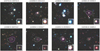	Fig. A.1. Sample of false color RGB (R = B_W, G = R, B = I) NDWFS images centered on spectroscopic quasars. Each image covers 70″ × 70″, and the inset size is 7″ × 7″. The contours are [3, 5, 7, 9, 11, 13] × σ times the local noise level in the LOFAR (white) and FIRST (purple) images.
Open with DEXTER

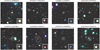	Fig. A.2. Sample of false color RGB (R = B_W, G = R, B = I) NDWFS images centered on photometric quasars. Each image covers 70″ × 70″, and the inset size is 7″ × 7″. The contours are [3, 5, 7, 9, 11, 13] × σ times the local noise level in the LOFAR (white) and FIRST (purple) images.
Open with DEXTER

All Tables

Table 1.

Properties of the training and target samples.

In the text

Table 2.

Performance of the classification algorithms for the quasar training sample.

In the text

Table 3.

Performance of the photometric redshifts for the quasar training sample.

In the text

Table 4.

Characteristics of the filters used in the NDWFS-Bootes field and their 3σ AB limiting magnitudes.

In the text

Table 5.

Binned luminosity functions for RSQs between 1.4 < z < 5.0.

In the text

Table 6.

Parametric model best-fit parameters and uncertainties.

In the text

All Figures

	Fig. 1. Transmission curves of the filters used in this work. Blue lines: SDSS-u and SDSS-r filters; red lines: the Pan-STARRS1 filter set: g_PS, r_PS, i_PS, z_PS, y_PS; green lines: Spitzer/IRAC [3.6 μm] and [4.5 μm] bands; purple lines: WISE W1 and W2 bands; and the solid black line shows a simulated quasar spectrum from our library at z = 3.4 (see Sect. 6.2).
Open with DEXTER
In the text

	Fig. 2. Photometric z_photo versus spectroscopic z_spec redshift for spectroscopic quasars in the NDWFS-Boötes region. The photometric redshifts are obtained using the NW kernel regression. The grey line indicates the one-to-one z_NW = z_spec relation, and the dashed-dotted and dashed lines indicate the z_NW − z_spec = ±0.10 × (1 + z_spec) and z_NW − z_spec = ±0.20 × (1 + z_spec) relations, respectively.
Open with DEXTER
In the text

	Fig. 3. Normalized histogram of the bias △z = z_phot − z_spec between photometric and spectroscopic redshifts for different samples. The phometric redshifts are obtained using the NW kernel regression. Around 76% of the spectroscopic quasars in the Boötes field have photometric redshifts that are correct within \|△z\| = 0.3 (see Table 3).
Open with DEXTER
In the text

	Fig. 4. Difference between the `PSF` and `cMODELMAG` magnitudes in the r band to separate point-like and extended sources as a function of redshift. The difference values are calculated considering the quantile that contains 95% of the quasars in the corresponding redshift bin. The redshift intervals match those used to derive the luminosity function in Sect. 6.4.
Open with DEXTER
In the text

	Fig. 5. Comparison between the colors of the training and NDWFS-Boötes (photometric and spectroscopic quasars) samples. Black contours and points denote the spectroscopic quasars with z > 1.4 of the training sample, while purple squares indicate all the spectroscopic quasars in Boötes with z > 1.4. Photometric quasars in our sample are denoted by red circles. The training sample is employed to identify quasars in the target sample (see Sect. 3), and to determine their photometric redshifts with the NW kernel regression method (see Sect. 4.1).
Open with DEXTER
In the text

	Fig. 6. Quasar colors versus redshift for different quasar samples between z = 1.4 and z = 5.5. Red points: RSQs with photometric redshifts; purple points: Boötes spectroscopic quasars; black contours and points: color distributions of the quasar training sample from Sect. 2.3; blue lines: mean color–redshift relations derived from the quasar training sample.
Open with DEXTER
In the text

	Fig. 7. Redshift distribution of photometric (red) and spectroscopic (blue) RSQs. Also, the combined redshift distribution (black) of photometric and spectroscopic RSQs is plotted.
Open with DEXTER
In the text

	Fig. 8. i_PS (top) and total flux S_150 MHz (bottom) distributions of photometric (red) and spectroscopic (blue) RSQs. Also, the combined redshift distribution (black) of photometric and spectroscopic RSQs is plotted. The method employed to select the quasars is described in Sect. 3.3.
Open with DEXTER
In the text

	Fig. 9. Absolute magnitude M₁₄₅₀ versus redshift for photometric (red) and spectroscopic (blue) RSQs in our sample. To minimize incompleteness due to incomplete M₁₄₅₀ bins while retaining the maximum numbers of quasars for estimating the luminosity function, we consider only RSQs with M₁₄₅₀ ≤ [−20.6,−21.8,−23.0] at 1.4 ≤ z < 2.4, 2.4 ≤ z < 3.1, and 3.1 ≤ z < 5.0; respectively. The dashed line denotes the magnitude limit i_PS = 23.0. This limit is calculated assuming a quasar continuum described by a power-law with slope α = −0.5 with no emission line contribution or Ly_α forest blanketing.
Open with DEXTER
In the text

	Fig. 10. Rest frame absolute luminosity density at 150 MHz versus redshift for photometric (red) and spectroscopic (blue) RSQs in our sample. The solid line denotes the 5σ flux limit (275 μJy) of the Boötes observations presented by Retana-Montenegro et al. (2018).
Open with DEXTER
In the text

	Fig. 11. Spectral energy distributions (SEDs) of four photometric quasars identified using our ML algorithms (see Sect. 3.3). The NDWFS-Boötes photometry is used to calculate the SEDs. In each case the best-fit quasar template (as derived from the EAZY calculation) is also plotted. Red circles are the photometric points and the blue circles indicate the predicted photometry by the best-fit template. The probability density distributions (PDFs) for each object are shown in the small inset. These PDFs strongly suggest that these objects are quasars located at z > 1.4.
Open with DEXTER
In the text

	Fig. 12. Normalized distributions of all NDWFS-Boötes spectroscopic quasars with z ≥ 1.4 (blue) and photometric (red) RSQs. See Sect. 5.2 for more details.
Open with DEXTER
In the text

	Fig. 13. Mid-infrared colors for photometric and spectroscopic quasars in the Boötes field. The photometric RSQs are plotted as red circles, while the spectroscopic quasars are indicated by purple circles. The light green lines are the mid-infrared color cuts proposed by Lacy et al. (2007) and Donley et al. (2012).
Open with DEXTER
In the text

	Fig. 14. Comparison of the χ² values for quasar, galaxy, and star template fitting to the photometry of spectroscopic quasars and candidate quasars in the NDWFS-Boötes field.
Open with DEXTER
In the text

	Fig. 15. Selection completeness, P_comp(i_PS,z ), binned according to magnitude i_PS and redshift z, in bins of size △i_PS = 0.5, and △z = 0.3, respectively.
Open with DEXTER
In the text

	Fig. 16. Ratio between the number of spectroscopic quasars with correctly and incorrectly assigned redshifts, f_photo-z, as a function of redshift. The redshift intervals match those used to derive the luminosity function in Sect. 6.4. The gray dashed line denotes the median value of f_photo-z.
Open with DEXTER
In the text

	Fig. 17. K-correction for different filters determined using our simulated quasar spectra. The Pan-STARRS1 r_PS and i_PS filters are indicated by blue and green, while the red and cyan are the expected K-corrections for the Pan-STARRS1 z_PS and SDSS-i bands. The solid black line is the K-correction assuming a power-law with slope α = −0.5 with no emission line contribution or Ly_α forest blanketing. At z ≳ 3.7, the difference between the r_PS and i_PS bands becomes more significant as the Ly_α line moves in or out of the filters. The same situation occurs at z ≳ 3.7, but for the i_PS and z_PS bands.
Open with DEXTER
In the text

	Fig. 18. Rest-frame M₁₄₅₀ binned luminosity functions of our Boötes RSQ samples (colored circles) for five non-overlapping redshift bins between 1.4 < z < 5.0. In each panel, we show as a reference the luminosity function at 1.65 < z < 2.4.
Open with DEXTER
In the text

	Fig. 19. Rest-frame M₁₄₅₀ binned luminosity functions of our Boötes RSQ samples (colored circles) for four non-overlapping redshift intervals between 1.4 < z < 5.0. The lines show the corresponding best-fit models in each redshift bin. The best-fitting parameters for each fit are presented in Table 6. For comparison, we show the QLFs from previous works (Cirasuolo et al. 2005; Siana et al. 2008; McGreer et al. 2009, 2018; Glikman et al. 2011; Masters et al. 2012; Ross et al. 2013; Giallongo et al. 2015; Tuccillo et al. 2015; Akiyama et al. 2018) measured over similar redshift intervals. The single-power law fits by McGreer et al. (2009) and Tuccillo et al. (2015) are plotted in the range −29 ≤ M₁₄₅₀ ≤ −26, which is the original range where they were measured.
Open with DEXTER
In the text

	Fig. 20. Best-fit quasar luminosity function parameters as a function of redshift. Our results are indicated by purple circles, while estimates from the literature (Siana et al. 2008; Glikman et al. 2011; Masters et al. 2012; Niida et al. 2016; Akiyama et al. 2018; Yang et al. 2018; McGreer et al. 2018) are represented by the corresponding symbols in the legend box. The red and gray lines represent the PLE and LEDE models from Ross et al. (2013), and the blue and dark cyan lines our PLE (1.4 < z < 2.4) and LEDE (2.4 < z < 5.0) models listed on Table 6. For clarity, we shift vertically the PLE and LEDE models from Ross et al. (2013) by a factor of +0.1 in the third panel.
Open with DEXTER
In the text

	Fig. 21. Spatial density of RSQs with M₁₄₅₀ < −22 as a function of redshift compared to the space density of faint quasar samples (M₁₄₅₀ < −22) from the literature. The spatial density of RSQs is indicated by purple circles, while estimates from the literature (Bongiorno et al. 2007; Siana et al. 2008; Glikman et al. 2011; Masters et al. 2012; Akiyama et al. 2018; Yang et al. 2018; McGreer et al. 2018) are represented by the corresponding symbols in the legend box. We also plot the spatial density of RSQs scaled by a factor of 5.0 (1/0.20) (blue circles).
Open with DEXTER
In the text

	Fig. 22. Left panel: spatial densities, normalized to z ∼ 2, as a function of redshift for optically faint quasars and RSQs. Our results are indicated by fuchsia circles, while the spatial density for faint quasars is determined from results reported in the literature (Bongiorno et al. 2007; Siana et al. 2008; Glikman et al. 2011; Masters et al. 2012; Akiyama et al. 2018; Yang et al. 2018) and is denoted by green triangles. The downward triangle indicates the spatial density excluding the results by Glikman et al. (2011) and Akiyama et al. (2018), while the value denoted the downward triangle includes them. Right panel: relative fraction of RSQs with respect to the spatial density of faint quasars as a function of redshift. The ratio is calculated between overlapping redshift bins. The gray solid line indicates the mean ratio of 0.22 excluding the works by Glikman et al. (2011) and Akiyama et al. (2018), while the dashed line denotes a mean ratio of 0.18 including these works.
Open with DEXTER
In the text

	Fig. A.1. Sample of false color RGB (R = B_W, G = R, B = I) NDWFS images centered on spectroscopic quasars. Each image covers 70″ × 70″, and the inset size is 7″ × 7″. The contours are [3, 5, 7, 9, 11, 13] × σ times the local noise level in the LOFAR (white) and FIRST (purple) images.
Open with DEXTER
In the text

	Fig. A.2. Sample of false color RGB (R = B_W, G = R, B = I) NDWFS images centered on photometric quasars. Each image covers 70″ × 70″, and the inset size is 7″ × 7″. The contours are [3, 5, 7, 9, 11, 13] × σ times the local noise level in the LOFAR (white) and FIRST (purple) images.
Open with DEXTER
In the text

Current usage metrics show cumulative count of Article Views (full-text article views including HTML views, PDF and ePub downloads, according to the available data) and Abstracts Views on Vision4Press platform.

Data correspond to usage on the plateform after 2015. The current usage metrics is available 48-96 hours after online publication and is updated daily on week days.

Initial download of the metrics may take a while.

[1] Abolfathi, B., Aguado, D. S., Aguilar, G., et al. 2018, ApJS, 235, 42 [NASA ADS] [CrossRef] [Google Scholar]

[2] Ahn, C. P., Alexandroff, R., Allende Prieto, C., et al. 2012, ApJS, 203, 21 [NASA ADS] [CrossRef] [Google Scholar]

[3] Aird, J., Coil, A. L., Georgakakis, A., et al. 2015, MNRAS, 451, 1892 [NASA ADS] [CrossRef] [Google Scholar]

[4] Akiyama, M., He, W., Ikeda, H., et al. 2018, PASJ, 70, S34 [NASA ADS] [CrossRef] [Google Scholar]

[5] Alexander, P. 2000, MNRAS, 319, 8 [NASA ADS] [CrossRef] [Google Scholar]

[6] Altman, N. S. 1992, Am. Stat., 46, 175 [Google Scholar]

[7] Ashby, M. L. N., Stern, D., Brodwin, M., et al. 2009, ApJ, 701, 428 [NASA ADS] [CrossRef] [Google Scholar]

[8] Assef, R. J., Kochanek, C. S., Ashby, M. L. N., et al. 2011, ApJ, 728, 56 [NASA ADS] [CrossRef] [Google Scholar]

[9] Bañados, E., Venemans, B. P., Morganson, E., et al. 2015, ApJ, 804, 118 [NASA ADS] [CrossRef] [Google Scholar]

[10] Baldwin, J. A. 1977, ApJ, 214, 679 [NASA ADS] [CrossRef] [Google Scholar]

[11] Becker, R. H., White, R. L., & Helfand, D. J. 1995, ApJ, 450, 559 [NASA ADS] [CrossRef] [Google Scholar]

[12] Becker, R. H., White, R. L., Gregg, M. D., et al. 2000, ApJ, 538, 72 [NASA ADS] [CrossRef] [Google Scholar]

[13] Bershady, M. A., Charlton, J. C., & Geoffroy, J. M. 1999, ApJ, 518, 103 [NASA ADS] [CrossRef] [Google Scholar]

[14] Bertin, E., & Arnouts, S. 1996, A&AS, 117, 393 [NASA ADS] [CrossRef] [EDP Sciences] [Google Scholar]

[15] Bian, F., Fan, X., Jiang, L., et al. 2013, ApJ, 774, 28 [NASA ADS] [CrossRef] [Google Scholar]

[16] Bongiorno, A., Zamorani, G., Gavignaud, I., et al. 2007, A&A, 472, 443 [NASA ADS] [CrossRef] [EDP Sciences] [Google Scholar]

[17] Bonzini, M., Padovani, P., Mainieri, V., et al. 2013, MNRAS, 436, 3759 [NASA ADS] [CrossRef] [Google Scholar]

[18] Boroson, T. A., & Green, R. F. 1992, ApJS, 80, 109 [NASA ADS] [CrossRef] [Google Scholar]

[19] Bovy, J., Hennawi, J. F., Hogg, D. W., et al. 2011, ApJ, 729, 141 [NASA ADS] [CrossRef] [Google Scholar]

[20] Boyle, B. J., Shanks, T., Croom, S. M., et al. 2000, MNRAS, 317, 1014 [NASA ADS] [CrossRef] [Google Scholar]

[21] Brammer, G. B., van Dokkum, P. G., & Coppi, P. 2008, ApJ, 686, 1503 [NASA ADS] [CrossRef] [Google Scholar]

[22] Breiman, L. 1996, Mach. Learn., 24, 123 [Google Scholar]

[23] Breiman, L. 2001, Mach. Learn., 45, 5 [CrossRef] [Google Scholar]

[24] Bridle, A. H., Hough, D. H., Lonsdale, C. J., Burns, J. O., & Laing, R. A. 1994, AJ, 108, 766 [NASA ADS] [CrossRef] [Google Scholar]

[25] Brotherton, M. S., & Francis, P. J. 1999, in Quasars and Cosmology, eds. G. Ferland, & J. Baldwin, ASP Conf. Ser., 162, 395 [NASA ADS] [Google Scholar]

[26] Brown, M. J. I., Brand, K., Dey, A., et al. 2006, ApJ, 638, 88 [NASA ADS] [CrossRef] [Google Scholar]

[27] Brown, M. J. I., Dey, A., Jannuzi, B. T., et al. 2007, ApJ, 654, 858 [NASA ADS] [CrossRef] [Google Scholar]

[28] Calzetti, D., Armus, L., Bohlin, R. C., et al. 2000, ApJ, 533, 682 [NASA ADS] [CrossRef] [Google Scholar]

[29] Campbell, J., Lo, A., & MacKinlay, A. 2012, The Econometrics of Financial Markets (Princeton: Princeton University Press) [CrossRef] [Google Scholar]

[30] Carballo, R., González-Serrano, J. I., Montenegro-Montes, F. M., et al. 2006, MNRAS, 370, 1034 [NASA ADS] [Google Scholar]

[31] Carrasco, D., Barrientos, L. F., Pichara, K., et al. 2015, A&A, 584, A44 [NASA ADS] [CrossRef] [EDP Sciences] [Google Scholar]

[32] Chabrier, G., Baraffe, I., Allard, F., & Hauschildt, P. 2000, ApJ, 542, 464 [NASA ADS] [CrossRef] [Google Scholar]

[33] Chambers, K. C., Magnier, E. A., Metcalfe, N., et al. 2016, ArXiv e-prints [arXiv:1612.05560] [Google Scholar]

[34] Chen, T., & Guestrin, C. 2016, ArXiv e-prints [arXiv:1603.02754] [Google Scholar]

[35] Cirasuolo, M., Magliocchetti, M., Celotti, A., & Danese, L. 2003, MNRAS, 341, 993 [NASA ADS] [CrossRef] [Google Scholar]

[36] Cirasuolo, M., Magliocchetti, M., & Celotti, A. 2005, MNRAS, 357, 1267 [NASA ADS] [CrossRef] [Google Scholar]

[37] Cirasuolo, M., Magliocchetti, M., Gentile, G., et al. 2006, MNRAS, 371, 695 [NASA ADS] [CrossRef] [Google Scholar]

[38] Coatman, L., Hewett, P. C., Banerji, M., & Richards, G. T. 2016, MNRAS, 461, 647 [NASA ADS] [CrossRef] [Google Scholar]

[39] Collier, J. D., Norris, R. P., Filipović, M. D., & Tothill, N. F. H. 2016, Astron. Nachr., 337, 36 [NASA ADS] [CrossRef] [Google Scholar]

[40] Condon, J. J., Kellermann, K. I., Kimball, A. E., Ivezić, Ž., & Perley, R. A. 2013, ApJ, 768, 37 [NASA ADS] [CrossRef] [Google Scholar]

[41] Cool, R. J. 2007, ApJS, 169, 21 [NASA ADS] [CrossRef] [Google Scholar]

[42] Cool, R. J., Kochanek, C. S., Eisenstein, D. J., et al. 2006, AJ, 132, 823 [NASA ADS] [CrossRef] [Google Scholar]

[43] Cortes, C., & Vapnik, V. 1995, Mach. Learn., 20, 273 [Google Scholar]

[44] Coziol, R., Andernach, H., Torres-Papaqui, J. P., Ortega-Minakata, R. A., & Moreno del Rio, F. 2017, MNRAS, 466, 921 [NASA ADS] [CrossRef] [Google Scholar]

[45] Cristiani, S., & Vio, R. 1990, A&A, 227, 385 [NASA ADS] [Google Scholar]

[46] Croom, S. M., Smith, R. J., Boyle, B. J., et al. 2001, MNRAS, 322, L29 [NASA ADS] [CrossRef] [Google Scholar]

[47] Croom, S. M., Smith, R. J., Boyle, B. J., et al. 2004, MNRAS, 349, 1397 [NASA ADS] [CrossRef] [Google Scholar]

[48] Croom, S. M., Richards, G. T., Shanks, T., et al. 2009a, MNRAS, 399, 1755 [NASA ADS] [CrossRef] [Google Scholar]

[49] Croom, S. M., Richards, G. T., Shanks, T., et al. 2009b, MNRAS, 392, 19 [NASA ADS] [CrossRef] [Google Scholar]

[50] Cutri, R. M. 2013, VizieR Online Data Catalog: II/328 [Google Scholar]

[51] Czerny, B., Li, J., Loska, Z., & Szczerba, R. 2004, MNRAS, 348, L54 [NASA ADS] [CrossRef] [Google Scholar]

[52] Dawson, K. S., Kneib, J.-P., Percival, W. J., et al. 2016, AJ, 151, 44 [NASA ADS] [CrossRef] [Google Scholar]

[53] DESI Collaboration (Aghamousa, A., et al.) 2016, ArXiv e-prints [arXiv:1611.00036] [Google Scholar]

[54] de Vries, W. H., Morganti, R., Röttgering, H. J. A., et al. 2002, AJ, 123, 1784 [NASA ADS] [CrossRef] [Google Scholar]

[55] de Vries, W. H., Becker, R. H., & White, R. L. 2006, AJ, 131, 666 [NASA ADS] [CrossRef] [Google Scholar]

[56] DiPompeo, M. A., Brotherton, M. S., De Breuck, C., & Laurent-Muehleisen, S. 2011, ApJ, 743, 71 [NASA ADS] [CrossRef] [Google Scholar]

[57] Donley, J. L., Koekemoer, A. M., Brusa, M., et al. 2012, ApJ, 748, 142 [NASA ADS] [CrossRef] [Google Scholar]

[58] Fan, X. 1999, AJ, 117, 2528 [NASA ADS] [CrossRef] [Google Scholar]

[59] Fan, X., Narayanan, V. K., Lupton, R. H., et al. 2001, AJ, 122, 2833 [NASA ADS] [CrossRef] [Google Scholar]

[60] Fanaroff, B. L., & Riley, J. M. 1974, MNRAS, 167, 31P [NASA ADS] [CrossRef] [Google Scholar]

[61] Fanti, C., Fanti, R., Schilizzi, R. T., Spencer, R. E., & van Breugel, W. J. M. 1986, A&A, 170, 10 [NASA ADS] [Google Scholar]

[62] Fanti, C., Fanti, R., Parma, P., et al. 1989, A&A, 217, 44 [NASA ADS] [Google Scholar]

[63] Fanti, R., Fanti, C., Schilizzi, R. T., et al. 1990, A&A, 231, 333 [NASA ADS] [Google Scholar]

[64] Fanti, C., Fanti, R., Dallacasa, D., et al. 1995, A&A, 302, 317 [NASA ADS] [Google Scholar]

[65] Flaugher, B. 2005, Int. J. Mod. Phys. A, 20, 3121 [NASA ADS] [CrossRef] [Google Scholar]

[66] Flesch, E. W. 2015, PASA, 32, e010 [NASA ADS] [CrossRef] [Google Scholar]

[67] Fontanot, F., Cristiani, S., Monaco, P., et al. 2007, A&A, 461, 39 [NASA ADS] [CrossRef] [EDP Sciences] [Google Scholar]

[68] Fukugita, M., Ichikawa, T., Gunn, J. E., et al. 1996, AJ, 111, 1748 [NASA ADS] [CrossRef] [Google Scholar]

[69] Gao, D., Zhang, Y.-X., & Zhao, Y.-H. 2008, MNRAS, 386, 1417 [NASA ADS] [CrossRef] [Google Scholar]

[70] Gavignaud, I., Bongiorno, A., Paltani, S., et al. 2006, A&A, 457, 79 [NASA ADS] [CrossRef] [EDP Sciences] [Google Scholar]

[71] Gehrels, N. 1986, ApJ, 303, 336 [NASA ADS] [CrossRef] [Google Scholar]

[72] Georgakakis, A., Aird, J., Buchner, J., et al. 2015, MNRAS, 453, 1946 [NASA ADS] [CrossRef] [Google Scholar]

[73] Giallongo, E., Grazian, A., Fiore, F., et al. 2015, A&A, 578, A83 [NASA ADS] [CrossRef] [EDP Sciences] [Google Scholar]

[74] Giallongo, E., Grazian, A., Fiore, F., et al. 2019, ApJ, 884, 19 [NASA ADS] [CrossRef] [Google Scholar]

[75] Glikman, E., Djorgovski, S. G., Stern, D., et al. 2011, ApJ, 728, L26 [NASA ADS] [CrossRef] [Google Scholar]

[76] Goldschmidt, P., Kukula, M. J., Miller, L., & Dunlop, J. S. 1999, ApJ, 511, 612 [NASA ADS] [CrossRef] [Google Scholar]

[77] Gunn, J. E., Siegmund, W. A., Mannery, E. J., et al. 2006, AJ, 131, 2332 [NASA ADS] [CrossRef] [Google Scholar]

[78] Gurkan, G., Hardcastle, M. J., Best, P. N., et al. 2019, A&A, 622, A11 [NASA ADS] [CrossRef] [EDP Sciences] [Google Scholar]

[79] Haardt, F., & Madau, P. 2012, ApJ, 746, 125 [NASA ADS] [CrossRef] [Google Scholar]

[80] Härdle, W. 1990, Applied Nonparametric Regression, Econometric Society Monographs (Cambridge: Cambridge University Press) [CrossRef] [Google Scholar]

[81] Hasinger, G., Miyaji, T., & Schmidt, M. 2005, A&A, 441, 417 [NASA ADS] [CrossRef] [EDP Sciences] [Google Scholar]

[82] Hatziminaoglou, E., Mathez, G., & Pelló, R. 2000, A&A, 359, 9 [NASA ADS] [Google Scholar]

[83] Herrera Ruiz, N., Middelberg, E., Norris, R. P., & Maini, A. 2016, A&A, 589, L2 [NASA ADS] [CrossRef] [EDP Sciences] [Google Scholar]

[84] Hertzsprung, E. 1909, Astron. Nachr., 179, 373 [NASA ADS] [CrossRef] [Google Scholar]

[85] Hodapp, K. W., Siegmund, W. A., Kaiser, N., et al. 2004, in Ground-based Telescopes, eds. J. Oschmann, & M. Jacobus, SPIE Conf. Ser., 5489, 667 [NASA ADS] [CrossRef] [Google Scholar]

[86] Hook, I. M., Shaver, P. A., & McMahon, R. G. 1998, in The Young Universe: Galaxy Formation and Evolution at Intermediate and High Redshift, eds. S. D’Odorico, A. Fontana, & E. Giallongo, ASP Conf. Ser., 146, 17 [NASA ADS] [Google Scholar]

[87] Hook, I. M., McMahon, R. G., Shaver, P. A., & Snellen, I. A. G. 2002, A&A, 391, 509 [NASA ADS] [CrossRef] [EDP Sciences] [Google Scholar]

[88] Ilbert, O., Arnouts, S., McCracken, H. J., et al. 2006, A&A, 457, 841 [NASA ADS] [CrossRef] [EDP Sciences] [Google Scholar]

[89] Ivezić, Ž., Menou, K., Knapp, G. R., et al. 2002, AJ, 124, 2364 [NASA ADS] [CrossRef] [Google Scholar]

[90] Ivezić, Ž., Brandt, W. N., Fan, X., et al. 2014, in Multiwavelength AGN Surveys and Studies, eds. A. M. Mickaelian, & D. B. Sanders, IAU Symp., 304, 11 [NASA ADS] [Google Scholar]

[91] Ivezić, Ž., Kahn, S. M., Tyson, J. A., et al. 2019, ApJ, 873, 111 [NASA ADS] [CrossRef] [Google Scholar]

[92] Jannuzi, B. T., & Dey, A. 1999, in Photometric Redshifts and the Detection of High Redshift Galaxies, eds. R. Weymann, L. Storrie-Lombardi, M. Sawicki, & R. Brunner, ASP Conf. Ser., 191, 111 [NASA ADS] [Google Scholar]

[93] Jannuzi, B., Weiner, B., Block, M., et al. 2010, in Amer. Astron. Soc. Meet. Abstr., #215, BAAS, 42, 513 [Google Scholar]

[94] Jiang, L., Fan, X., Ivezić, Ž., et al. 2007, ApJ, 656, 680 [NASA ADS] [CrossRef] [Google Scholar]

[95] Jiang, L., McGreer, I. D., Fan, X., et al. 2016, ApJ, 833, 222 [NASA ADS] [CrossRef] [Google Scholar]

[96] Jin, X., Zhang, Y., Zhang, J., et al. 2019, MNRAS, 485, 4539 [NASA ADS] [CrossRef] [Google Scholar]

[97] Kashikawa, N., Ishizaki, Y., Willott, C. J., et al. 2015, ApJ, 798, 28 [NASA ADS] [CrossRef] [Google Scholar]

[98] Kellermann, K. I., Sramek, R., Schmidt, M., Shaffer, D. B., & Green, R. 1989, AJ, 98, 1195 [NASA ADS] [CrossRef] [Google Scholar]

[99] Kennefick, J. D., Djorgovski, S. G., & de Carvalho, R. R. 1995, AJ, 110, 2553 [NASA ADS] [CrossRef] [Google Scholar]

[100] Kenter, A., Murray, S. S., Forman, W. R., et al. 2005, ApJS, 161, 9 [NASA ADS] [CrossRef] [Google Scholar]

[101] Kimball, A. E., Knapp, G. R., Ivezić, Ž., et al. 2009, ApJ, 701, 535 [NASA ADS] [CrossRef] [Google Scholar]

[102] Kimball, A. E., Kellermann, K. I., Condon, J. J., Ivezić, Ž., & Perley, R. A. 2011, ApJ, 739, L29 [NASA ADS] [CrossRef] [Google Scholar]

[103] Kirkpatrick, J. A., Schlegel, D. J., Ross, N. P., et al. 2011, ApJ, 743, 125 [NASA ADS] [CrossRef] [Google Scholar]

[104] Kochanek, C. S., Eisenstein, D. J., Cool, R. J., et al. 2012, ApJS, 200, 8 [NASA ADS] [CrossRef] [Google Scholar]

[105] Kratzer, R. M., & Richards, G. T. 2015, AJ, 149, 61 [NASA ADS] [CrossRef] [Google Scholar]

[106] Kunert-Bajraszewska, M., Cegłowski, M., Katarzyński, K., & Roskowiński, C. 2015, A&A, 579, A109 [NASA ADS] [CrossRef] [EDP Sciences] [Google Scholar]

[107] Lacy, M., Wilson, G., Masci, F., et al. 2005, ApJS, 161, 41 [NASA ADS] [CrossRef] [Google Scholar]

[108] Lacy, M., Petric, A. O., Sajina, A., et al. 2007, AJ, 133, 186 [NASA ADS] [CrossRef] [Google Scholar]

[109] La Franca, F., Gregorini, L., Cristiani, S., de Ruiter, H., & Owen, F. 1994, AJ, 108, 1548 [NASA ADS] [CrossRef] [Google Scholar]

[110] Laureijs, R., Amiaux, J., Arduini, S., et al. 2011, ArXiv e-prints [arXiv:1110.3193] [Google Scholar]

[111] Le Fèvre, O., Cassata, P., Cucciati, O., et al. 2013, A&A, 559, A14 [NASA ADS] [CrossRef] [EDP Sciences] [Google Scholar]

[112] Li, Q., & Racine, J. 2011, Nonparametric Econometrics: Theory and Practice (Princeton: Princeton University Press) [Google Scholar]

[113] Liu, Y., Jiang, D. R., Wang, T. G., & Xie, F. G. 2008, MNRAS, 391, 246 [NASA ADS] [CrossRef] [Google Scholar]

[114] Lonsdale, C. J., Smith, H. E., Rowan-Robinson, M., et al. 2003, PASP, 115, 897 [NASA ADS] [CrossRef] [Google Scholar]

[115] LSST Science Collaboration (Abell, P. A., et al.) 2009, ArXiv e-prints [arXiv:0912.0201] [Google Scholar]

[116] Lu, Y., Wang, T., Zhou, H., & Wu, J. 2007, AJ, 133, 1615 [NASA ADS] [CrossRef] [Google Scholar]

[117] Lupton, R. H., Gunn, J. E., & Szalay, A. S. 1999, AJ, 118, 1406 [NASA ADS] [CrossRef] [Google Scholar]

[118] Maddox, N., Hewett, P. C., Péroux, C., Nestor, D. B., & Wisotzki, L. 2012, MNRAS, 424, 2876 [NASA ADS] [CrossRef] [Google Scholar]

[119] Magnier, E. A., Sweeney, W. E., Chambers, K. C., et al. 2016, ArXiv e-prints [arXiv:1612.05244] [Google Scholar]

[120] Martin, D. C., Fanson, J., Schiminovich, D., et al. 2005, ApJ, 619, L1 [NASA ADS] [CrossRef] [Google Scholar]

[121] Masters, D., Capak, P., Salvato, M., et al. 2012, ApJ, 755, 169 [NASA ADS] [CrossRef] [Google Scholar]

[122] Masters, D., Capak, P., Stern, D., et al. 2015, ApJ, 813, 53 [NASA ADS] [CrossRef] [Google Scholar]

[123] Mauduit, J. C., Lacy, M., Farrah, D., et al. 2012, PASP, 124, 1135 [NASA ADS] [CrossRef] [Google Scholar]

[124] McGreer, I. D., Becker, R. H., Helfand, D. J., & White, R. L. 2006, ApJ, 652, 157 [NASA ADS] [CrossRef] [Google Scholar]

[125] McGreer, I. D., Helfand, D. J., & White, R. L. 2009, AJ, 138, 1925 [NASA ADS] [CrossRef] [Google Scholar]

[126] McGreer, I. D., Jiang, L., Fan, X., et al. 2013, ApJ, 768, 105 [NASA ADS] [CrossRef] [Google Scholar]

[127] McGreer, I. D., Fan, X., Jiang, L., & Cai, Z. 2018, AJ, 155, 131 [NASA ADS] [CrossRef] [Google Scholar]

[128] Meisner, A. M., Lang, D., & Schlegel, D. J. 2017, AJ, 154, 161 [NASA ADS] [CrossRef] [Google Scholar]

[129] Messias, H., Afonso, J., Salvato, M., Mobasher, B., & Hopkins, A. M. 2012, ApJ, 754, 120 [NASA ADS] [CrossRef] [Google Scholar]

[130] Miller, L., Peacock, J. A., & Mead, A. R. G. 1990, MNRAS, 244, 207 [NASA ADS] [Google Scholar]

[131] Miyaji, T., Hasinger, G., Salvato, M., et al. 2015, ApJ, 804, 104 [NASA ADS] [CrossRef] [Google Scholar]

[132] Møller, P., & Jakobsen, P. 1990, A&A, 228, 299 [NASA ADS] [Google Scholar]

[133] Morabito, L. K., Deller, A. T., Röttgering, H., et al. 2016, MNRAS, 461, 2676 [NASA ADS] [CrossRef] [Google Scholar]

[134] Morabito, L. K., Matthews, J. H., Best, P. N., et al. 2019, A&A, 622, A15 [NASA ADS] [CrossRef] [EDP Sciences] [Google Scholar]

[135] Mullin, L. M., Riley, J. M., & Hardcastle, M. J. 2008, MNRAS, 390, 595 [NASA ADS] [CrossRef] [Google Scholar]

[136] Myers, A. D., Palanque-Delabrouille, N., Prakash, A., et al. 2015, ApJS, 221, 27 [NASA ADS] [CrossRef] [Google Scholar]

[137] Nadaraya, E. 1964, Theory Probab. Appl., 9, 141 [CrossRef] [Google Scholar]

[138] Nakoneczny, S., Bilicki, M., Solarz, A., et al. 2019, A&A, 624, A13 [NASA ADS] [CrossRef] [EDP Sciences] [Google Scholar]

[139] Niida, M., Nagao, T., Ikeda, H., et al. 2016, ApJ, 832, 208 [NASA ADS] [CrossRef] [Google Scholar]

[140] Norris, R. P. 2017, Nat. Astron., 1, 671 [NASA ADS] [CrossRef] [Google Scholar]

[141] Norris, R. P., Hopkins, A. M., Afonso, J., et al. 2011, PASA, 28, 215 [NASA ADS] [CrossRef] [Google Scholar]

[142] O’Dea, C. P. 1998, PASP, 110, 493 [NASA ADS] [CrossRef] [Google Scholar]

[143] Oke, J. B., & Gunn, J. E. 1983, ApJ, 266, 713 [NASA ADS] [CrossRef] [Google Scholar]

[144] Orienti, M., Dallacasa, D., & Stanghellini, C. 2007, A&A, 461, 923 [NASA ADS] [CrossRef] [EDP Sciences] [Google Scholar]

[145] Padovani, P. 1993, MNRAS, 263, 461 [NASA ADS] [Google Scholar]

[146] Padovani, P., Miller, N., Kellermann, K. I., et al. 2011, ApJ, 740, 20 [NASA ADS] [CrossRef] [Google Scholar]

[147] Palanque-Delabrouille, N., Magneville, C., Yèche, C., et al. 2016, A&A, 587, A41 [NASA ADS] [CrossRef] [EDP Sciences] [Google Scholar]

[148] Papovich, C., Cool, R., Eisenstein, D., et al. 2006, AJ, 132, 231 [NASA ADS] [CrossRef] [Google Scholar]

[149] Papovich, C., Shipley, H. V., Mehrtens, N., et al. 2016, ApJS, 224, 28 [NASA ADS] [CrossRef] [Google Scholar]

[150] Pâris, I., Petitjean, P., Aubourg, É., et al. 2018, A&A, 613, A51 [NASA ADS] [CrossRef] [EDP Sciences] [Google Scholar]

[151] Pasquet, J., Bertin, E., Treyer, M., Arnouts, S., & Fouchez, D. 2019, A&A, 621, A26 [NASA ADS] [CrossRef] [EDP Sciences] [Google Scholar]

[152] Pasquet-Itam, J., & Pasquet, J. 2018, A&A, 611, A97 [NASA ADS] [CrossRef] [EDP Sciences] [Google Scholar]

[153] Peacock, J. A., & Wall, J. V. 1982, MNRAS, 198, 843 [NASA ADS] [Google Scholar]

[154] Peacock, J. A., Miller, L., & Longair, M. S. 1986, MNRAS, 218, 265 [NASA ADS] [Google Scholar]

[155] Pei, Y. C. 1992, ApJ, 395, 130 [NASA ADS] [CrossRef] [Google Scholar]

[156] Pei, Y. C. 1995, ApJ, 438, 623 [NASA ADS] [CrossRef] [Google Scholar]

[157] Peng, N., Zhang, Y., Zhao, Y., & Wu, X.-B. 2012, MNRAS, 425, 2599 [NASA ADS] [CrossRef] [Google Scholar]

[158] Peters, C. M., Richards, G. T., Myers, A. D., et al. 2015, ApJ, 811, 95 [NASA ADS] [CrossRef] [Google Scholar]

[159] Prandoni, I., de Ruiter, H. R., Ricci, R., et al. 2010, A&A, 510, A42 [NASA ADS] [CrossRef] [EDP Sciences] [Google Scholar]

[160] Pu, X. 2013, Ap&SS, 345, 355 [NASA ADS] [CrossRef] [Google Scholar]

[161] Qiu, P. 2013, Introduction to Statistical Process Control, Chapman & Hall/CRC Texts in Statistical Science (CRC Press) [CrossRef] [Google Scholar]

[162] Retana-Montenegro, E., & Röttgering, H. J. A. 2017, A&A, 600, A97 [NASA ADS] [CrossRef] [EDP Sciences] [Google Scholar]

[163] Retana-Montenegro, E., & Röttgering, H. 2018, Front. Astron. Space Sci., 5, 5 [NASA ADS] [CrossRef] [Google Scholar]

[164] Retana-Montenegro, E., Röttgering, H. J. A., Shimwell, T. W., et al. 2018, A&A, 620, A74 [NASA ADS] [CrossRef] [EDP Sciences] [Google Scholar]

[165] Richards, G. T., Weinstein, M. A., Schneider, D. P., et al. 2001, AJ, 122, 1151 [NASA ADS] [CrossRef] [Google Scholar]

[166] Richards, G. T., Fan, X., Newberg, H. J., et al. 2002, AJ, 123, 2945 [NASA ADS] [CrossRef] [Google Scholar]

[167] Richards, G. T., Strauss, M. A., Fan, X., et al. 2006, AJ, 131, 2766 [NASA ADS] [CrossRef] [Google Scholar]

[168] Richards, G. T., Myers, A. D., Gray, A. G., et al. 2009, ApJS, 180, 67 [NASA ADS] [CrossRef] [Google Scholar]

[169] Richards, G. T., Kruczek, N. E., Gallagher, S. C., et al. 2011, AJ, 141, 167 [NASA ADS] [CrossRef] [Google Scholar]

[170] Richards, G. T., Myers, A. D., Peters, C. M., et al. 2015, ApJS, 219, 39 [NASA ADS] [CrossRef] [Google Scholar]

[171] Ross, N. P., McGreer, I. D., White, M., et al. 2013, ApJ, 773, 14 [NASA ADS] [CrossRef] [Google Scholar]

[172] Röttgering, H., Afonso, J., Barthel, P., et al. 2011, JApA, 32, 557 [NASA ADS] [CrossRef] [Google Scholar]

[173] Russell, H. N. 1914, Pop. Astron., 22, 275 [NASA ADS] [Google Scholar]

[174] Salvato, M., Hasinger, G., Ilbert, O., et al. 2009, ApJ, 690, 1250 [NASA ADS] [CrossRef] [Google Scholar]

[175] Sanders, D. B., Salvato, M., Aussel, H., et al. 2007, ApJS, 172, 86 [NASA ADS] [CrossRef] [Google Scholar]

[176] Schindler, J.-T., Fan, X., McGreer, I. D., et al. 2017, ApJ, 851, 13 [NASA ADS] [CrossRef] [Google Scholar]

[177] Schlafly, E. F., & Finkbeiner, D. P. 2011, ApJ, 737, 103 [NASA ADS] [CrossRef] [Google Scholar]

[178] Schmidt, M. 1968, ApJ, 151, 393 [NASA ADS] [CrossRef] [Google Scholar]

[179] Schmidt, M., Schneider, D. P., & Gunn, J. E. 1995, AJ, 110, 68 [NASA ADS] [CrossRef] [Google Scholar]

[180] Schneider, D. P., Richards, G. T., Hall, P. B., et al. 2010, AJ, 139, 2360 [NASA ADS] [CrossRef] [Google Scholar]

[181] Schulze, A., Done, C., Lu, Y., Zhang, F., & Inoue, Y. 2017, ApJ, 849, 4 [NASA ADS] [CrossRef] [Google Scholar]

[182] Scranton, R., Johnston, D., Dodelson, S., et al. 2002, ApJ, 579, 48 [NASA ADS] [CrossRef] [Google Scholar]

[183] Shaver, P. A., Wall, J. V., Kellermann, K. I., Jackson, C. A., & Hawkins, M. R. S. 1996, Nature, 384, 439 [NASA ADS] [CrossRef] [Google Scholar]

[184] Shen, Y., Strauss, M. A., Ross, N. P., et al. 2009, ApJ, 697, 1656 [NASA ADS] [CrossRef] [Google Scholar]

[185] Shimwell, T. W., Röttgering, H. J. A., Best, P. N., et al. 2017, A&A, 598, A104 [NASA ADS] [CrossRef] [EDP Sciences] [Google Scholar]

[186] Shimwell, T. W., Tasse, C., Hardcastle, M. J., et al. 2019, A&A, 622, A1 [NASA ADS] [CrossRef] [EDP Sciences] [Google Scholar]

[187] Siana, B., Polletta, M. D. C., Smith, H. E., et al. 2008, ApJ, 675, 49 [NASA ADS] [CrossRef] [Google Scholar]

[188] Sikora, M. 2009, Astron. Nachr., 330, 291 [NASA ADS] [CrossRef] [Google Scholar]

[189] Sikora, M., Stawarz, Ł., & Lasota, J.-P. 2007, ApJ, 658, 815 [NASA ADS] [CrossRef] [Google Scholar]

[190] Silverman, J. D., Green, P. J., Barkhouse, W. A., et al. 2005, ApJ, 624, 630 [NASA ADS] [CrossRef] [Google Scholar]

[191] Smith, J. D., Thompson, D., & Djorgovski, S. 1993, in Sky Surveys. Protostars to Protogalaxies, ed. B. T. Soifer, ASP Conf. Ser., 43, 189 [NASA ADS] [Google Scholar]

[192] Snellen, I. A. G., Schilizzi, R. T., Miley, G. K., et al. 2000, MNRAS, 319, 445 [NASA ADS] [CrossRef] [Google Scholar]

[193] Somerville, R. S., Hopkins, P. F., Cox, T. J., Robertson, B. E., & Hernquist, L. 2008, MNRAS, 391, 481 [NASA ADS] [CrossRef] [Google Scholar]

[194] Spergel, D., Gehrels, N., Breckinridge, J., et al. 2013, ArXiv e-prints [arXiv:1305.5422] [Google Scholar]

[195] Spergel, D., Gehrels, N., Baltay, C., et al. 2015, ArXiv e-prints [arXiv:1503.03757] [Google Scholar]

[196] Stern, D., Djorgovski, S. G., Perley, R. A., de Carvalho, R. R., & Wall, J. V. 2000, AJ, 119, 1526 [NASA ADS] [CrossRef] [Google Scholar]

[197] Stern, D., Eisenhardt, P., Gorjian, V., et al. 2005, ApJ, 631, 163 [NASA ADS] [CrossRef] [Google Scholar]

[198] Stocke, J. T., Morris, S. L., Weymann, R. J., & Foltz, C. B. 1992, ApJ, 396, 487 [NASA ADS] [CrossRef] [Google Scholar]

[199] Sulentic, J., & Marziani, P. 2015, Front. Astron. Space Sci., 2, 6 [NASA ADS] [CrossRef] [Google Scholar]

[200] Sulentic, J. W., Marziani, P., & Dultzin-Hacyan, D. 2000a, ARA&A, 38, 521 [NASA ADS] [CrossRef] [Google Scholar]

[201] Sulentic, J. W., Zwitter, T., Marziani, P., & Dultzin-Hacyan, D. 2000b, ApJ, 536, L5 [NASA ADS] [CrossRef] [Google Scholar]

[202] Sulentic, J. W., Zamfir, S., Marziani, P., et al. 2003, ApJ, 597, L17 [NASA ADS] [CrossRef] [Google Scholar]

[203] Sulentic, J. W., Bachev, R., Marziani, P., Negrete, C. A., & Dultzin, D. 2007, ApJ, 666, 757 [NASA ADS] [CrossRef] [Google Scholar]

[204] Telfer, R. C., Zheng, W., Kriss, G. A., & Davidsen, A. F. 2002, ApJ, 565, 773 [NASA ADS] [CrossRef] [Google Scholar]

[205] Timlin, J. D., Ross, N. P., Richards, G. T., et al. 2016, ApJS, 225, 1 [NASA ADS] [CrossRef] [Google Scholar]

[206] Timlin, J. D., Ross, N. P., Richards, G. T., et al. 2018, ApJ, 859, 20 [NASA ADS] [CrossRef] [Google Scholar]

[207] Tonry, J. L., Stubbs, C. W., Lykke, K. R., et al. 2012, ApJ, 750, 99 [NASA ADS] [CrossRef] [Google Scholar]

[208] Trump, J. R., Impey, C. D., Elvis, M., et al. 2009, ApJ, 696, 1195 [NASA ADS] [CrossRef] [Google Scholar]

[209] Tuccillo, D., González-Serrano, J. I., & Benn, C. R. 2015, MNRAS, 449, 2818 [NASA ADS] [CrossRef] [Google Scholar]

[210] Tyson, J. A. 2002, in Survey and Other Telescope Technologies and Discoveries, eds. J. A. Tyson, & S. Wolff, Proc. SPIE, 4836, 10 [NASA ADS] [CrossRef] [Google Scholar]

[211] Ueda, Y., Akiyama, M., Ohta, K., & Miyaji, T. 2003, ApJ, 598, 886 [NASA ADS] [CrossRef] [Google Scholar]

[212] van Breugel, W., Miley, G., & Heckman, T. 1984, AJ, 89, 5 [NASA ADS] [CrossRef] [Google Scholar]

[213] van Haarlem, M. P., Wise, M. W., Gunst, A. W., et al. 2013, A&A, 556, A2 [NASA ADS] [CrossRef] [EDP Sciences] [Google Scholar]

[214] Vanden Berk, D. E., Richards, G. T., Bauer, A., et al. 2001, AJ, 122, 549 [NASA ADS] [CrossRef] [Google Scholar]

[215] Varenius, E., Conway, J. E., Martí-Vidal, I., et al. 2015, A&A, 574, A114 [NASA ADS] [CrossRef] [EDP Sciences] [Google Scholar]

[216] Vasconcellos, E. C., de Carvalho, R. R., Gal, R. R., et al. 2011, AJ, 141, 189 [NASA ADS] [CrossRef] [Google Scholar]

[217] Vigotti, M., Carballo, R., Benn, C. R., et al. 2003, ApJ, 591, 43 [NASA ADS] [CrossRef] [Google Scholar]

[218] Visnovsky, K. L., Impey, C. D., Foltz, C. B., et al. 1992, ApJ, 391, 560 [NASA ADS] [CrossRef] [Google Scholar]

[219] Vito, F., Gilli, R., Vignali, C., et al. 2014, MNRAS, 445, 3557 [NASA ADS] [CrossRef] [Google Scholar]

[220] Volonteri, M., & Rees, M. J. 2005, ApJ, 633, 624 [NASA ADS] [CrossRef] [Google Scholar]

[221] Wang, D., Zhang, Y. X., Liu, C., & Zhao, Y. H. 2007, MNRAS, 382, 1601 [NASA ADS] [CrossRef] [Google Scholar]

[222] Warren, S. J., Hewett, P. C., & Osmer, P. S. 1994, ApJ, 421, 412 [NASA ADS] [CrossRef] [Google Scholar]

[223] Watson, G. S. 1964, Sankhya: Indian J. Stat. Ser. A (1961–2002), 26, 359 [Google Scholar]

[224] Weinstein, M. A., Richards, G. T., Schneider, D. P., et al. 2004, ApJS, 155, 243 [NASA ADS] [CrossRef] [Google Scholar]

[225] Welling, C. A., Miller, B. P., Brandt, W. N., Capellupo, D. M., & Gibson, R. R. 2014, MNRAS, 440, 2474 [NASA ADS] [CrossRef] [Google Scholar]

[226] Williams, W. L., Intema, H. T., & Röttgering, H. J. A. 2013, A&A, 549, A55 [NASA ADS] [CrossRef] [EDP Sciences] [Google Scholar]

[227] Williams, W. L., van Weeren, R. J., Röttgering, H. J. A., et al. 2016, MNRAS, 460, 2385 [NASA ADS] [CrossRef] [Google Scholar]

[228] Willott, C. J., Delorme, P., Reylé, C., et al. 2010, AJ, 139, 906 [NASA ADS] [CrossRef] [Google Scholar]

[229] Wolf, C., Wisotzki, L., Borch, A., et al. 2003, A&A, 408, 499 [NASA ADS] [CrossRef] [EDP Sciences] [Google Scholar]

[230] Wright, E. L., Eisenhardt, P. R. M., Mainzer, A. K., et al. 2010, AJ, 140, 1868 [NASA ADS] [CrossRef] [Google Scholar]

[231] Wu, H., & Zhang, J. 2006, Nonparametric Regression Methods for Longitudinal Data Analysis: Mixed-Effects Modeling Approaches (Wiley Press) [Google Scholar]

[232] Yang, Q., Wu, X.-B., Fan, X., et al. 2017, AJ, 154, 269 [NASA ADS] [CrossRef] [Google Scholar]

[233] Yang, J., Wu, X.-B., Liu, D., et al. 2018, AJ, 155, 110 [NASA ADS] [CrossRef] [Google Scholar]

[234] Yao, S., Wu, X.-B., Ai, Y. L., et al. 2019, ApJS, 240, 6 [NASA ADS] [CrossRef] [Google Scholar]

[235] Yèche, C., Petitjean, P., Rich, J., et al. 2010, A&A, 523, A14 [NASA ADS] [CrossRef] [EDP Sciences] [Google Scholar]

[236] York, D. G., Adelman, J., Anderson, Jr., J. E., et al. 2000, AJ, 120, 1579 [NASA ADS] [CrossRef] [Google Scholar]

[237] Zakamska, N. L., & Greene, J. E. 2014, MNRAS, 442, 784 [NASA ADS] [CrossRef] [Google Scholar]

[238] Zakamska, N. L., Lampayan, K., Petric, A., et al. 2016, MNRAS, 455, 4191 [NASA ADS] [CrossRef] [Google Scholar]

[239] Zamfir, S., Sulentic, J. W., & Marziani, P. 2008, MNRAS, 387, 856 [NASA ADS] [CrossRef] [Google Scholar]

[240] Zeimann, G. R., White, R. L., Becker, R. H., et al. 2011, ApJ, 736, 57 [NASA ADS] [CrossRef] [Google Scholar]

The optical luminosity function of LOFAR radio-selected quasars at 1.4 ≤ z ≤ 5.0 in the NDWFS-Boötes field⋆

1. Introduction

2. Data

2.1. NOAO Deep Wide-field survey

2.2. SDSS, Pan-STARRS1, WISE, and Spitzer surveys

2.3. Spectroscopic quasars with optical and mid-infrared photometry

3. Classification

3.1. Training sample

3.2. Target sample

3.3. Classification algorithms

3.3.1. Random forest

3.3.2. Support vector machines

3.3.3. Bootstrap aggregation on K-nearest neighbors

3.3.4. Performance

3.3.5. Classification results

3.3.6. Radio data

4. Photometric redshifts

4.1. Nadaraya–Watson kernel regression

4.2. Quasar training sample

4.3. Redshift estimation

5. Quasar sample

5.1. Final sample

5.2. Spectral energy distribution of photometric quasars

5.3. Cross-matching to X-ray data

5.4. Density of photometric quasars

5.5. LOFAR and wedge-based mid-infrared selection of quasars

6. Luminosity function of radio-selected quasars

6.1. Selection completeness and accuracy of photometric redshifts

6.2. Simulated Quasar Spectra

6.3. K-correction

6.4. Quasar Luminosity function

7. Results

7.1. Model-fitting

7.2. Comparison to previous works

7.3. Density evolution of RSQs

8. Discussion

8.1. The origins of radio-emission in RSQs

8.2. The environment of RSQs

8.3. RSQs and their location in spectroscopic parameter spaces

9. Conclusions

Acknowledgments

References

Appendix A: A sample of false color RGB (R = BW, G = R, B = I) images

All Tables

All Figures

The optical luminosity function of LOFAR radio-selected quasars at 1.4 ≤ z ≤ 5.0 in the NDWFS-Boötes field^⋆

Appendix A: A sample of false color RGB (R = B_W, G = R, B = I) images