| Issue |
A&A
Volume 633, January 2020
|
|
|---|---|---|
| Article Number | A66 | |
| Number of page(s) | 15 | |
| Section | The Sun | |
| DOI | https://doi.org/10.1051/0004-6361/201936944 | |
| Published online | 14 January 2020 | |
Nonequilibrium ionization and ambipolar diffusion in solar magnetic flux emergence processes⋆
1
Rosseland Centre for Solar Physics, University of Oslo, PO Box 1029, Blindern 0315, Oslo, Norway
e-mail: desiveri@astro.uio.no
2
Institute of Theoretical Astrophysics, University of Oslo, PO Box 1029, Blindern 0315, Oslo, Norway
3
Instituto de Astrofisica de Canarias, Via Lactea, s/n, 38205 La Laguna, Tenerife, Spain
4
Department of Astrophysics, Universidad de La Laguna, 38200 La Laguna, Tenerife, Spain
5
Bay Area Environmental Research Institute, NASA Research Park, Moffett Field, CA 94952, USA
6
Lockheed Martin Solar and Astrophysics Laboratory, Palo Alto, CA 94304, USA
Received:
17
October
2019
Accepted:
27
November
2019
Context. Magnetic flux emergence from the solar interior has been shown to be a key mechanism for unleashing a wide variety of phenomena. However, there are still open questions concerning the rise of the magnetized plasma through the atmosphere, mainly in the chromosphere, where the plasma departs from local thermodynamic equilibrium (LTE) and is partially ionized.
Aims. We aim to investigate the impact of the nonequilibrium (NEQ) ionization and recombination and molecule formation of hydrogen, as well as ambipolar diffusion, on the dynamics and thermodynamics of the flux emergence process.
Methods. Using the radiation-magnetohydrodynamic Bifrost code, we performed 2.5D numerical experiments of magnetic flux emergence from the convection zone up to the corona. The experiments include the NEQ ionization and recombination of atomic hydrogen, the NEQ formation and dissociation of H2 molecules, and the ambipolar diffusion term of the generalized Ohm’s law.
Results. Our experiments show that the LTE assumption substantially underestimates the ionization fraction in most of the emerged region, leading to an artificial increase in the ambipolar diffusion and, therefore, in the heating and temperatures as compared to those found when taking the NEQ effects on the hydrogen ion population into account. We see that LTE also overestimates the number density of H2 molecules within the emerged region, thus mistakenly magnifying the exothermic contribution of the H2 molecule formation to the thermal energy during the flux emergence process. We find that the ambipolar diffusion does not significantly affect the amount of total unsigned emerged magnetic flux, but it is important in the shocks that cross the emerged region, heating the plasma on characteristic times ranging from 0.1 to 100 s. We also briefly discuss the importance of including elements heavier than hydrogen in the equation of state so as not to overestimate the role of ambipolar diffusion in the atmosphere.
Key words: Sun: atmosphere / Sun: chromosphere / Sun: magnetic fields / methods: numerical
Movies associated to Figs. 2–5, 8, 9, and A.1 are available at https://www.aanda.org
© ESO 2020
1. Introduction
Magnetic flux emergence is a fundamental process that brings magnetic field from the solar interior to the atmosphere. It is key not only in understanding the solar magnetic activity, but also in improving our predictions of space weather events: many prominent features in the solar atmosphere are related to this fundamental mechanism. From the theoretical perspective, magnetic flux emergence has been addressed from different points of view. Some authors have focused on the rise of the magnetized plasma through the convection zone, first by means of idealized magnetohydrodynamics (MHD) experiments of the rise of twisted magnetic tube through stratified media (see, e.g., Moreno-Insertis & Emonet 1996; Longcope et al. 1996; Emonet & Moreno-Insertis 1998; Martínez-Sykora et al. 2015a, and references therein), and then through radiation-MHD experiments that include a self-consistent convection zone, (e.g., Martínez-Sykora et al. 2008; Tortosa-Andreu & Moreno-Insertis 2009; Moreno-Insertis et al. 2018, among others). For instance, Cheung et al. (2007) showed that granular motions can strongly modify the rise of the magnetized tubes, deforming, slowing down, and even breaking them into separate strands. This means that the pattern of arrival of the magnetized plasma at the surface critically depends on the evolution of the flux emergence in the solar interior. Other authors have analyzed the interaction of the emerging plasma with the preexisting coronal field: from early numerical simulations by Forbes & Priest (1984), Shibata et al. (1992), Yokoyama & Shibata (1995, 1996) to the most recent ones (see, e.g., Moreno-Insertis & Galsgaard 2013; Fang et al. 2014; MacTaggart et al. 2015; Nóbrega-Siverio et al. 2016; Hansteen et al. 2017; Ni et al. 2017; Zhao et al. 2018; Yang et al. 2018; Hansteen et al. 2019). The interaction between the emerged magnetic plasma and the ambient field can be manifested in many ways, such as: (a) the impulsive release of mass and energy that may constitute a significant input to the upper solar atmosphere and to the solar wind (Raouafi et al. 2016); (b) the formation of strong shocks and the generation of turbulence (Priest 2014); (c) nonthermal processes and the acceleration of particles (Priest & Forbes 2002); (d) and quasi-periodic radio emission due to tearing instabilities and coalescence of plasmoids in the current sheet (Karlický et al. 2010). The interaction between the emerged region and the preexisting coronal field can even provide telltale signatures about the structure of the magnetic fields below the surface, which is a useful diagnostic tool for the solar dynamo (Cheung & Isobe 2014). All of those implications make magnetic flux emergence a vibrant and active research area. In spite of the continued theoretical effort, there are still open questions concerning this fundamental process. Flux emergence processes occur through various layers in the Sun in which many different physical mechanisms are involved, and where usually several assumptions are made to be able to deal with the complexity of those layers. As Leenaarts et al. (2018) recently pointed out, flux emergence numerical experiments including radiation and the interaction between ions and neutrals have not been reported so far. In fact, basic questions are still unanswered like, for instance, how the energy is transported and dissipated in the chromosphere and, more generally, which physical ingredients are necessary for a realistic model of emerging flux.
A common assumption in numerical experiments of the Sun is to model the plasma using the MHD approximation in which the plasma is treated as a single fluid with complete coupling between its constituent microscopic species. This approximation is able to successfully explain many phenomena in different solar contexts; nonetheless, there are regions and phenomena where this assumption is no longer valid because, for example, the plasma is partially ionized and there is a decrease in the collisional coupling (Zweibel et al. 2011; Khomenko & Collados 2012; Martínez-Sykora et al. 2015b; Zweibel 2015; Shelyag et al. 2016; Ballester et al. 2018, among others). There is a way to relax the MHD approximations to still treat the plasma as a single fluid but including the mentioned effects: the generalized Ohm’s law (see the fundamental books by Braginskii 1965; Mitchner & Kruger 1973; Cowling 1976 and its implementation in codes by, e.g., Leake et al. 2005; O’Sullivan & Downes 2007; Cheung & Cameron 2012; Martínez-Sykora et al. 2012; González-Morales et al. 2018). Numerical experiments with this extension report a large impact of the interaction between neutrals and ions in the lower solar atmosphere. For instance, this interaction is key to getting type II spicules and misalignment between the thermal and magnetic structures in the chrosmosphere (Martínez-Sykora et al. 2016a, 2017a,b); it is able to damp Alfvén waves in the chromosphere (De Pontieu et al. 2001; Leake et al. 2005; Soler et al. 2015; Cally & Khomenko 2018; Khomenko & Cally 2019); and it also affects the onset of instabilities (Khomenko et al. 2014; Ruderman et al. 2018). In particular, for magnetic flux emergence processes, the ambipolar diffusion and the associated Pedersen dissipation have been shown to counteract, to some extent, the cooling during the expansion of the magnetized plasma in the atmosphere and to lead to the slippage of the magnetic field with respect to the bulk plasma velocity, thus increasing the total magnetic flux that emerges in the solar atmosphere (Leake & Arber 2006; Arber et al. 2007; Leake & Linton 2013). However, those computations including partial ionization effects were carried out assuming a plasma constituted only by hydrogen and using moreover a simple model based on the modified Saha equation to calculate departures from local thermodynamic equilibrium (LTE) instead of a fully nonequilibrium (NEQ) ionization calculation.
Important departures from the ionization equilibrium in the solar atmosphere have been predicted by theory for several decades now. The seminal papers by Klein et al. (1976, 1978), Kneer (1980), Carlsson & Stein (1992, 2002), among others, showed by means of 1D simulations that ionization in shocks occurs on a faster timescale than recombination behind them. On the contrary, in LTE, almost all thermal energy is suddenly gone into ionization or taken from recombination, so less temperature increase is reached in the postshocks in comparison with the NEQ case. Major improvements in the computational capabilities have provided a much more complete perspective of the NEQ processes in the chromosphere and transition region. For example, Leenaarts & Wedemeyer-Böhm (2006), Leenaarts et al. (2007, 2011) and Golding et al. (2014, 2016) explored, through 2D and 3D numerical experiments, the large thermodynamical variations in the chromosphere due to the NEQ ionization and recombination of hydrogen and helium. From those works, it was concluded that the ionization degree of hydrogen and helium and, consequently, the electron density cannot be calculated in the chromosphere using the LTE approximation. Other authors have shown that heavy ions also suffer important departures from LTE, for instance, by means of 1D hydrodynamic simulations in coronal loops, nanoflares and other impulsive events (Bradshaw & Mason 2003; Bradshaw & Cargill 2006; Bradshaw & Klimchuk 2011; Reep et al. 2016, 2018); or in multidimensional radiation-MHD experiments that additionally included spectral synthesis to explain different observational features in the transition region (Olluri et al. 2013, 2015; De Pontieu et al. 2015; Martínez-Sykora et al. 2016b) or in solar phenomena like surges (Nóbrega-Siverio et al. 2017, 2018). Relaxing the LTE condition is therefore important when considering the ionization degree of the most abundant species, especially since the free electron and ion number density influence, for example, the radiative losses in the atmosphere. Hansteen (1993) found deviations of more than a factor two in the optically thin losses in a 1D nanoflare model when considering NEQ effects. See also the dependence on the number density of different elements in the chromospheric radiative loss expressions proposed by Carlsson & Leenaarts (2012).
The aim of this paper is to analyze the role of the NEQ ionization and recombination and partial ionization, namely, the effects due to the ion-neutral interactions, during the emergence of the magnetized plasma in the chromosphere. The layout of the paper is as follows. Section 2 contains the description of the underlying magnetic flux emergence numerical model. Section 3 shows the main results of the paper, focusing on the ionization fraction, temperature, and molecular fraction within the emerged region (Sect. 3.1), the shocks within the emerged region and the associated ambipolar diffusion heating (Sect. 3.2), and the amount of magnetic flux that emerges from the solar interior (Sect. 3.3). Finally, Sect. 4 summarizes and discusses the main conclusions of the present work, as well as the limitations of the present work.
2. Physical and numerical model
For this paper, we have run 2.5D numerical flux emergence experiments. The details of the underlying model are divided into four sections: the numerical code and the specific modules enabled for the present calculations (Sect. 2.1); the background stratification and the boundary conditions (Sect. 2.2); the properties of the twisted magnetic tube injected to produce flux emergence (Sect. 2.3); and the initial stages and branches of the experiments (Sect. 2.4).
2.1. The numerical code
The numerical experiments were performed using the 3D radiation-MHD Bifrost code (Gudiksen et al. 2011). This code takes radiative transfer with scattering into account (Skartlien 2000; Hayek et al. 2010), includes the most important radiative gains and losses in the chromosphere due to the strong lines from hydrogen, calcium and magnesium (Carlsson & Leenaarts 2012), apart from optically thin losses and thermal conduction along the magnetic field in the corona. To prevent the plasma from cooling down to low temperatures where the radiation and equation-of-state (EOS) tables of the code are not accurate, there is an ad hoc heating term that forces the temperature to stay above T = 1660 K. In addition to the above, we use the two following modules which are the main ones for this manuscript.
2.1.1. NEQ ionization recombination and molecule formation of hydrogen
We have enabled a module for the Bifrost code that computes the NEQ ionization and recombination of hydrogen using a 6-level atom that contains five excitation states for the neutral hydrogen and the ionized level. This module also calculates the formation and dissociation of molecular hydrogen, H2, under NEQ conditions (see Leenaarts et al. 2007, 2011, for details about this module).
2.1.2. Generalized Ohm’s law (GOL)
We have also used a module that extends the classical Ohm’s law to include partial ionization effects. In particular, we have used a new version of the generalized Ohm’s law (GOL) module developed by Nóbrega-Siverio et al. (in prep.) that improves the capabilities of the original one (Martínez-Sykora et al. 2012) by implementing the Super-Time-Stepping (STS) method (Alexiades et al. 1996). This method allows us to relax the CFL criterion (Courant et al. 1928), which imposes large restrictions on the timestep, to accelerate the explicit calculation of the ambipolar diffusion term, which is crucial in magnetic flux emergence experiments. In the following, the main equations in this module are briefly summarized.
In the laboratory reference frame, it can be shown (see, e.g., Mitchner & Kruger 1973) that the generalized Ohm’s law (GOL) is given by

where u is the plasma velocity, E the electric field, B the magnetic field, and J the current density all measured in that reference frame. The coefficient η is the standard ohmic diffusion given by

the ambipolar diffusion coefficient, ηamb,
and the Hall coefficient, ηHall,

where qe is the electron charge; ne the number density of electrons; me the electron mass; ρN the total neutral mass density obtained from the different neutrals n considered, that is, ρN = Σnρn; ρ the total mass density; νe, ni the total collision frequency of electrons with neutrals and ions; and  the reduced neutral-ion collision frequency (see, e.g., Goodman 2000) given by
with ni the ion number density; KB the Boltzmann’s constant, T the temperature, and mni = mnmi/(mn + mi) the reduced mass of the neutral and ion species. The temperature-dependent cross section between a given neutral and charged particle (ion or electron), σni, is implemented following Vranjes & Krstic (2013) for hydrogen and helium. For the elastic cross section for hydrogen protons colliding with H2 molecules we use Krstic & Schultz (1999). The rest of the collision cross sections follows the same assumptions made by Vranjes et al. (2008) for heavy ions: we take the cross section between hydrogen (or helium) and protons multiplied by mi/mH (or mi/mHe).
In this work, the Hall term was not considered. This term is perpendicular to the electric current J, so it does not play a direct role in the heating due to dissipation. Moreover, neglecting this term facilitates the comparison with previous papers where magnetic flux emergence was studied with ambipolar diffusion but without the Hall term (Leake & Arber 2006; Arber et al. 2007; Leake & Linton 2013). With respect to the Ohmic diffusion, it is negligible in comparison with the numerical diffusion of the code (see, e.g., Martínez-Sykora et al. 2012, 2017b, for a comparison of the different GOL terms). For this reason, Ohm’s term is not included in Bifrost: neither in the classical Ohm’s law nor in the GOL extension. Instead, a hyper-diffusion term, ηhypJ, is implemented, where ηhyp is the hyper-diffusion coefficient (for details, see Gudiksen et al. 2011).
2.2. The background stratification and boundary conditions
We started from a statistically stationary two-dimensional snapshot that encompasses from the uppermost layers of the solar convection zone to the corona. The relaxation of this snapshot was carried out including all the physics mentioned above, with the exception of the NEQ module. The latter is enabled coinciding with the injection of the magnetic twisted tube through the lower boundary (see Sect. 2.4 for details).
The physical domain of the numerical box is 0 ≤ x ≤ 32 Mm and −2.87 ≤ z ≤ 14.2 Mm, where z = 0 Mm corresponds to the horizontal layer where ⟨τ500⟩ ≈ 1, with τ500 being the optical depth at 500 nm. The domain is solved with 2048 × 1000 grid cells using a uniform numerical grid in both the horizontal and vertical directions with Δx ≈ 16 km and Δz ≈ 17 km, respectively. Concerning the boundary conditions, they are periodic in the horizontal direction. For the vertical direction, the bottom boundary is open and prescribes constant entropy for the incoming plasma; and the top one uses characteristic boundary conditions (see Gudiksen et al. 2011). Furthermore, in the corona we have added a hot-plate that forces a fixed temperature in the top cells. In this case, we fix the temperature to stay around 6 × 10⁵ K. This value could seem low for the corona, but since we are interested in the details within the emerged region, the results are not affected by this fact.
Panel A in Fig. 1 shows the horizontal averages of the stratification of the statistically stationary initial snapshot for temperature T (green), magnetic field B (black), gas pressure P (blue), and density ρ (red). The stratification curves in the figure are normalized to the photospheric values at z = 0 Mm, namely, Tph = 5803 K, Bph = 0.44 G, Pph = 1.12 × 10⁵ erg cm−3, and ρph = 3.20 × 10⁻⁷ g cm−3. Panel B of that figure contains a 2D temperature map for the initial snapshot (t = 0 min). In this initial snapshot we have chosen the magnetic field to be very weak: (1) to allow an easier analysis, since the only magnetized plasma in the atmosphere is the one that has emerged; and (2) to prevent any important magnetic reconnection episode between the emerged plasma and the preexisting ambient field in the atmosphere, so no hot ejections, surges or other eruptive and explosive phenomena can perturb the emerged region.
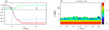 |
Fig. 1. Properties of the initial snapshot (t = 0 min). Panel A: horizontal averages of the initial stratification for temperature T (green), magnetic field strength B (black), pressure P (blue) and density ρ (red) normalized to their photospheric values at z = 0 Mm (Tph = 5803 K, Bph = 0.44 G, Pph = 1.12 × 10⁵ erg cm−3, and ρph = 3.20 × 10⁻⁷ g cm−3). The dotted vertical line delineates the solar surface. Panel B: 2D map for the initial background stratification of the temperature only showing values below T = 3 × 10⁴ K. The solar surface is roughly at z = 0 Mm (dashed horizontal black line). The other dashed line is an isocontour that delimits the transition region at T = 105 K. |
2.3. The twisted magnetic tube
In order to produce flux emergence, we injected in the initial snapshot (t = 0 min) a twisted magnetic tube. The axis of the tube points in the y-direction, and the longitudinal and transverse components of the magnetic field have the following canonical form (see, e.g., Fan 2001):


where B0 is the magnetic field in the axis of the tube, q a constant twist parameter, r and θ are, respectively, the radial and azimuthal coordinates with respect to the tube axis, and R0 is the tube radius.
The tube is injected through the bottom boundary following the method described by Martínez-Sykora et al. (2008). This method prescribes the magnetic field at the boundaries, updating the height of the tube every timestep according to the average vertical speed of the inflow plasma, uz, where the tube is located. The electric field of the tube is then computed following Ohm’s law (e.g., for the x-component Ex = By uz) preserving the solenoidality condition ∇ ⋅ B = 0.
We set up two flux emergence experiments with the same parameters for the magnetic tube, namely, B0 = 20 kG, q = 2.4 Mm−1, and R0 = 0.1 Mm. Those parameters were selected to get an initial axial magnetic flux of Φ0 = 6.3 × 10¹⁸ Mx, which is in the lower range of an ephemeral active region (Zwaan 1987), and leads to a coherent emergence pattern at the surface. The initial height of the tube is set at z0 = −3.1 Mm for both experiments. The only difference between the two experiments is the horizontal location x0 where the tube is injected (see also first column in Table 1). This is because the pattern of arrival of the magnetized plasma at the surface critically depends on the interaction of the tube with the cells in the interior and, hence, on x0. For Experiment 1 we used x0 = 12.5 Mm. For Experiment 2 we used x0 = 13.0 Mm.
Scheme of the time evolution for the two experiments and the physical mechanisms included at the different stages.
2.4. Initial stages and branches of the experiments
The experiments begin with the injection of the twisted magnetic tube through the bottom boundary of the numerical box (t = 0 min). In that instant, we switched on the NEQ module. Since the tube is injected deep enough in the convection zone, all the transients in the atmosphere related to enabling the NEQ module would have disappeared before the tube reaches the surface: the timescales of those transients are small (about a hundred seconds Leenaarts et al. 2007) compared with the time that the twisted tube takes to rise through the convection zone (tens of minutes). In addition, the NEQ and the ambipolar diffusion effects are negligible in the convection zone, so the rise and expansion of the magnetic tube in this region are similar to our previous experiments where we did not include any of those physical mechanisms (Nóbrega-Siverio et al. 2016, 2018), namely, the tube rises with velocities of a few km s−1; the convection flows deform and break the twisted magnetic tube into smaller fragments; and, finally, part of the twisted tube reaches the surface. In the experiments of the present paper, the rise from the injection point up to the surface takes roughly 50 min. There, the magnetized plasma starts to pile up producing anomalous magnetized granules. To understand the NEQ and ambipolar diffusion effects in the subsequent evolution, from t = 60 min ondward, for both experiments we create the following four branches:
-
NEQ+AD: here we continue the experiment without changes, in other words, using the NEQ and ambipolar diffusion modules.
-
NEQ: in this branch we turn off the ambipolar diffusion.
-
LTE+AD: here we turn off the NEQ module but keep the ambipolar diffusion.
-
LTE: in this branch we use neither the NEQ nor the ambipolar diffusion modules, so the ionization is computed under the LTE assumption and we use the classical Ohm’s law.
This way we can separate and understand the role of the different physical mechanisms in the flux emergence process. The instant to create those branches has been carefully chosen as close as possible to the beginning of the phase of emergence through the chromosphere, in order to have similar structures in the preexisting atmosphere and thus be able to perform one-to-one comparisons between branches. Also we have tried to start the branching not too late in time for the NEQ and ambipolar diffusion effects to be negligible in the emerging plasma, and so avoid affecting the subsequent results with our choice (see Appendix A for further details). Disabling those modules introduces some transients in the chromosphere; nonetheless they vanish faster than the timescale for the emergence process within the chromosphere. The evolution of the experiments is summarized in Table 1.
3. Results
When the magnetized plasma of the twisted tube reaches the surface, the magnetic field piles up there and the magnetic pressure increases. Its later evolution occurs through the development of the buoyancy instability (Newcomb 1961), which allows the magnetized plasma to rise well above the photospheric heights. The magnetized plasma thus expands into the atmosphere giving rise to dome-like structures akin in shape to the ones in previous experiments (e.g., Archontis et al. 2004; Moreno-Insertis 2006; Nóbrega-Siverio et al. 2018). In our case, Experiment 1 leads to two emerged domes that interact with each other, similarly to, for example, Hansteen et al. (2019); while Experiment 2 gives rise to a single dome as in the paper by Nóbrega-Siverio et al. (2016). In the following, we analyze the emerged region for the four branches (LTE, LTE+AD, NEQ, NEQ+AD) of the two experiments.
3.1. Ionization fraction, temperature, and molecular fraction in the emerged region
In order to analyze the role of both the NEQ populations of atomic and molecular hydrogen and the ambipolar diffusion, we first focus on (a) the ionization fraction, ρi/ρ, which is a good tracer of the relevance of the nonequilibrium ionization and recombination as well as of the ambipolar diffusion term since its coefficient depends on the number density of neutrals and ions (see Eq. (3)); (b) the temperature, T; and (c) the fraction of molecular hydrogen, fH2, given by
where we consider that our hydrogen atom model consists of 6 levels (see Sect. 2.1.1). Figures 2 and 3 show the emerged region for Experiment 1 and 2, respectively. The four rows of the images are for the different branches (LTE, LTE+AD, NEQ, and NEQ+AD), while the three columns contain, from left to right, ρi/ρ, T, and fH2.
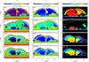 |
Fig. 2. Emerged region for Experiment 1. The rows contain the four branches of this experiment, namely, in descending order, LTE, LTE+AD, NEQ, NEQ+AD. From left to right columns: ionization fraction, ρi/ρ; the temperature, T; and the fraction of molecular hydrogen, fH2. Dashed lines indicate the location of the solar surface (line at z = 0 Mm) and of the transition region (isocontour at T = 105 K). Solid white isocontours delimit the temperature threshold limit at T = 1660 K. An animation of this figure is available online. |
The LTE case (first row of Figs. 2 and 3, and their respectively online animations) shows an extremely low degree of ionization (ρi/ρ < 10−4) in most of the interior of the domes, except for a vertical region in Experiment 1, where the two emerged domes are colliding and a current sheet is being created between them; and in Experiment 2 around x = 15 Mm, in the shock front explained in Sect. 3.2. Concerning the temperature, the emerged domes suffer strong cooling during their expansion with the result that, in Experiment 1, most of the dome is at the threshold temperature value where ad-hoc heating is activated (see white solid isocontours at T = 1660 K). Experiment 2 also shows temperatures at that threshold but to a lesser extent.
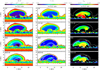 |
Fig. 3. Emerged region for Experiment 2. The rows contain the four branches of this experiment, namely, in descending order, LTE, LTE+AD, NEQ, NEQ+AD. From left to right columns: ionization fraction, ρi/ρ; the temperature, T; and the fraction of molecular hydrogen, fH2. Dashed lines indicate the location of the solar surface (line at z = 0 Mm) and of the transition region (isocontour at T = 105 K). Solid white isocontours delimit the temperature threshold limit at T = 1660 K. An animation of this figure is available online. |
With respect to the H2 molecules, we find that they constitute around 70% of the total hydrogen content by mass within the emerged region. This means that for an LTE case, not even the high exothermic contribution of the H2 molecule formation (4.48 eV per molecule) is able to counteract the cooling during the flux emergence through the atmosphere.
When including ambipolar diffusion in the LTE case (second row of Figs. 2 and 3), we notice several differences. The ionization fraction within the domes is now much larger than in the previous case: in Experiment 1, this is evident in almost the whole emerged region; while in Experiment 2, it is visible in a bubble-like structure in the inner core. The reason for this increase in both experiments is the role of the ambipolar diffusion related to the shocks that pass through the domes and that we describe in Sect. 3.2. The temperature in this branch is also greater; in fact, we get temperatures at least 100 K above the threshold limit during the whole process of emergence (as we can note by the lack of white solid contours at T = 1660 K in comparison with other branches). In this case, the ad hoc heating is not necessary at any stage of the flux emergence process. With respect to fH2, as a consequence of the larger temperatures in comparison with the LTE branch, the formation of molecules is substantially reduced in most of the emerged region. In fact, the molecules are limited to small regions in the core of the domes; the maximum value of fH2 is around 60%.
The NEQ branch (third row of Figs. 2 and 3) shows a larger ρi/ρ in most of the emerged region than the LTE branch, meaning that the assumption of LTE leads to wrong values of the real ionization fraction. This result also impacts on the calculation of the ambipolar diffusion coefficient since  : in the upper part of the domes, the assumption of LTE overestimates ni and hence the role of ambipolar diffusion. Regarding the temperature, in the NEQ branch the threshold limit T = 1660 K is reached to an even larger extent than in the LTE branch, especially in Experiment 2. In both experiments we see prominent arch-like structures with T ≈ 3 × 10³ K embedded in the cool T = 1660 K domain. They correspond to shock fronts; their importance is discussed in the next section. With respect to the molecules, in NEQ there are more ions so the formation rate of H2 is less important than in LTE. The maximum molecular fraction fH2 is around 27% and only located in the inner part of the domes. This implies that the LTE assumption vastly overestimates the number density of molecules and, therefore, their corresponding thermostatic action in magnetic flux emergence episodes.
For the NEQ+AD case (fourth row of Figs. 2 and 3), the ionization and molecular fraction are practically identical to the NEQ branch without ambipolar diffusion just discussed.
The main difference between NEQ+AD and NEQ can be found in the areas surrounding the arch-like structures associated with shocks mentioned before. The inclusion of ambipolar diffusion seems to offset some of the strong cooling during the expansion of the emerged region; however it is not enough to avoid reaching the temperature threshold at T = 1660 K, and, therefore, those domes are affected by the ad-hoc heating.
3.2. Shocks within the emerged region and the role of the ambipolar diffusion heating
To locate the shock fronts propagating in the domain, in particular those already mentioned in the previous paragraphs, we use the divergence of the plasma velocity field ∇ ⋅ u as a marker. In Fig. 4 (and associated movie), we show this quantity for the NEQ+AD branch of both experiments at different stages of the evolution. In the image, arrows have been added that point to specific cases of interest in the emerged region. In all the branches of the two experiments, during the rise of the magnetized plasma through the solar corona, several compression waves go through the emerged domes and steepen into shocks. Their origin is diverse: the turbulent motion of the convection zone, secondary magnetic flux emergence episodes, even the non-stationary reconnection between domes (Experiment 1). We have found that the strongest shocks leave an important imprint in the emerged dome, especially in the experiment branches that take the ambipolar diffusion into account. To show this in detail we use Experiment 2, in which the structure of the shock is simpler. Figure 5 contains the emerged region for that experiment at different instants (rows). The left column of the image shows the temperature T for the NEQ branch; the middle column contains T for the NEQ+AD case; and the right column shows, also for NEQ+AD, the characteristic time of the ambipolar diffusion heating τqamb, which is defined by
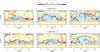 |
Fig. 4. Divergence of the plasma velocity field, ∇ ⋅ u, for Experiments 1 (top) and 2 (bottom) at different stages of the magnetic flux emergence process. Arrows are superimposed pointing out the location of some of the shocks within the emerged regions. Dashed lines indicate the location of the solar surface (line at z = 0 Mm) and of the transition region (isocontour at T = 105 K). An animation of this figure is available online. |
where e is the internal energy per unit volume, qamb is the ambipolar diffusion heating, and J⊥ is the current perpendicular to the magnetic field.
Taking a look at the left and middle columns of Fig. 5, we can appreciate that there is a prominent front that traverses the dome and, in spite of the energy expended in dissociation and ionization processes in the shock, results in a marked temperature jump between the pre-shock and post-shock regions (see also the associated animation). The temperature increase in the NEQ+AD branch is greater, and the width of the relaxation region behind the shock wider, than in the purely NEQ branch. In fact, in the right column of Fig. 5, we can see that the characteristic times of the ambipolar diffusion heating τqamb associated with the shock are small compared to the evolutionary timescales of the emergence process, implying that the heating is very efficient. In order to better illustrate this, a slanted solid line, which is nearly perpendicular to the shock front at the different instants, has been superimposed in all the panels of Fig. 5. Thus, we can analyze the profiles of different quantities along that cut, so as to quantify the significance of the shock. The corresponding profiles are shown in Fig. 6. The left column, panels A, B and C, of the image contains the evolution of the temperature T (black lines, left axis) and the ionization fraction ρi/ρ (blue lines, right axis) for the NEQ case (long dashed lines) and NEQ+AD (solid ones). Additionally, the threshold temperature where the ad-hoc heating is activated (T = 1660 K) is shown with a horizontal dash-dotted line in red. In those panels, it is clear that the jumps are larger when including ambipolar diffusion; they can be up to a factor two greater for the NEQ+AD case as compared to that with only NEQ. For the ionization fraction, the jump is even greater, reaching roughly a factor of one order of magnitude. The shock in either branch moves with an average speed of ∼18 km s−1. The panels in the right column of Fig. 6 (A.1, B.1, and C.1) contain a zoom of the gray region of the left panels, showing again the evolution of the temperature in the shock (for context purposes), but now in the right axis we plot the characteristic time of the ambipolar diffusion heating, τqamb (orange), together with the characteristic compression time of the shock, τcomp (blue lines), given by
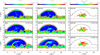 |
Fig. 5. Shock evolution within the emerged region for the Experiment 2 at different instants (rows). Left column: temperature, T, for the NEQ branch; middle column: T for the NEQ+AD case; and right column: characteristic time of the heating due to ambipolar diffusion, τqamb (see Eq. (9)). In addition, a solid line nearly perpendicular to the shock front has been superimposed in all the panels to study the variation of different quantities due to the shock passage (see Fig. 6). In the image, dashed lines indicate the location of the solar surface (line at z = 0 Mm) and of the transition region (isocontour at T = 105 K). An animation of this figure is available online. |
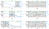 |
Fig. 6. Evolution of different quantities along the cut plotted in Fig. 5 for the same instants reproduced in that image. The x and z coordinates along that line are given as abscissas in the bottom and top axes, respectively. Left panels: evolution of the temperature T (black lines, left axis) and ionization fraction ρi/ρ (blue lines, right axis) for the NEQ case (long dashed lines) and NEQ+AD (solid ones). Right panels: zoom of the gray region of the left panels. The curves are for the temperature (black), and the characteristic times τcomp (blue) and τqamb (orange), keeping the long dashed lines for the purely NEQ case and solid lines for the NEQ + AD one. The tick-marks for the temperature are given on the left axis, and those for the times on the right axis. For all panels, the threshold temperature, T = 1660 K, is shown with a horizontal dash-dotted line in red. |
(in the plot, only the values in compression regions, ∇ ⋅ u < 0, are shown). In all cases, the compression time τcomp is within a factor two of 10 s, on the order of the time of passage of the plasma through the shock. On the other hand, in the first panel of the right column (t = 73.0 min), the ambipolar diffusion heating time, τqamb, is as small as ∼0.1 s, almost two orders of magnitude smaller than τcomp: this indicates that the ambipolar diffusion clearly plays a role in increasing the internal energy of the plasma as it crosses the shock, even if part of that increase is consumed in hydrogen ionization or molecule dissociation rather than in raising the temperature. Eighteen seconds later (at t = 73.3 min), τqamb is still below 1 s, that is, about one order of magnitude shorter than τcomp. It is only in the third panel of the right column (at t = 73.8 min) that τqamb is near to (even though still smaller than) τcomp. The short characteristic values for τqamb obtained in the NEQ+AD case explain the significant departures seen in the thermal evolution across the shock in that branch with respect to the NEQ branch. Considering the passage of the shock through the whole dome, which lasts for some ∼100 s, we expect the effects of the ambipolar diffusion to be noticeable in changing the temperature, and the molecular and atomic H fractions, of the plasma, as we have seen to be the case in the previous section and figures.
3.3. Magnetic field slippage
Hitherto, we have studied the dissipation due to ambipolar diffusion and how it affects the temperature. In this section, inspired by previous numerical papers about flux emergence including ion-neutral interaction effects (Leake & Arber 2006; Arber et al. 2007; Leake & Linton 2013), we study a second aspect related to ambipolar diffusion: we consider whether there is mutual slippage between the magnetic field lines and the bulk plasma flow in our experiments. To that end, the unsigned vertical flux, namely,
was computed for the four branches (LTE, LTE+AD, NEQ, NEQ+AD) of Experiment 1 and 2 at different heights: z = [0.5,1.0,2.0,3.0,4.0,5.0] Mm. The integration is calculated over the whole horizontal domain, so x0 = 0 Mm and xf = 32 Mm, for 15 min after the start of the branches at t = 60 min. We also define rΦ as the relative difference of the unsigned vertical flux between the branches with and without ambipolar diffusion:
and compute the average, ⟨rΦ⟩, and standard deviation, σrΦ, for those 15 min after the start of the branches. The results are shown in Fig. 7 and Table 2.
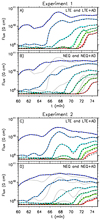 |
Fig. 7. Unsigned vertical flux Φ as a function of time during the flux emergence process for Experiment 1 (panels A and B) and Experiment 2 (panels C and D) for different heights, namely, z = [0.5,1.0,2.0,3.0,4.0,5.0] Mm. The LTE panel for each experiment contains |


Panel A of the figure shows the vertical magnetic flux for the LTE+AD branch,  , (colored solid lines) and the LTE case, ΦLTE, (superimposed dashed lines) for different heights in Experiment 1. As can bee seen,
  and ΦLTE are almost identical, regardless of the height. The relative difference between fluxes is less than around 2%. In addition, the standard deviation is a factor 2−3 of the mean value, which indicates that there is a large variation in the ratio between both magnetic fluxes, with the LTE flux sometimes being larger than the LTE+AD one, as seen for z = 0.5 Mm, where ⟨rΦ⟩ is negative. From this result, it seems that the ambipolar diffusion produces a negligible effect in the amount of emerged flux under the LTE assumption.
The second panel from the top contains the magnetic flux for the NEQ+AD branch,  , (colored solid lines) and the NEQ case, ΦNEQ, (superimposed dashed lines) for Experiment 1. We can again see that the magnetic flux in both cases is practically identical, no matter the height. In fact, the corresponding statistical values in Table 2 show that when considering NEQ, the relative difference is even smaller than in LTE, finding that the average is close to 0. The conclusion is that the magnetic slippage due to ambipolar diffusion, as measured by the ⟨rΦ⟩ parameter, is also negligible when enabling the NEQ module. Panel B of Fig. 7 also shows
  (gray curves) for comparison purposes between the LTE and NEQ cases. For this experiment, it seems that at the lower heights, z = 0.5 and z = 1.0 Mm, the magnetic flux emerges sooner in NEQ than in LTE, while the opposite behavior is found for the other heights. In spite of this fact, at t ≈ 75 min both NEQ and LTE fluxes converge to roughly the same value at the different heights, with the largest difference being found at z = 5.0 Mm.
The two remaining panels in Fig. 7 (panels C and D) are the equivalent plots for Experiment 2. Those panels illustrate the same features explained for Experiment 1: the ambipolar diffusion has no significant impact on the emerged magnetic flux, neither in NEQ nor in LTE, which can be also checked through the corresponding statistical values in Table 2.
A test has also been carried out checking for variations in the amount of chromospheric plasma that rises during the magnetic flux emergence process. To that end, we have performed the same kind of analysis like for the magnetic flux: we have calculated the integral
for the same heights as before, namely z = [0.5,1.0,2.0,3.0,4.0,5.0] Mm. The quantity Ψ is the integrated column density along the given horizontal level; monitoring Ψ may help discover any deviation in the amount of emerged plasma between the different cases. In fact, we find that there is no significant difference in the amount of mass lifted by the emergence process when including the ambipolar diffusion or otherwise, which is a natural consequence of the lack of magnetic field slippage previously found.
In order to understand the aforementioned lack of magnetic field slippage, we have to take a look at the drift velocity uamb, which measures the departure of the ion velocity from the bulk plasma velocity u and is given by
The order of magnitude of |uamb| is thus given by three factors: (a) the square of |B|/ρ; (b) a somewhat complicated expression whose spatial variation, however, in most cases is just given by that of the ratio ρn/ρi; and (c) the inverse of the characteristic length of the magnetic field  . The module of the remaining term,
  , is expected to be of order one, since the electric current in the emerged domes is nearly perpendicular to the magnetic field. In the following, we analyze these blocks using Experiment 2 to illustrate with examples.
The left column of Fig. 8 shows the ratio |B|2/ρ2 at three different stages of the flux emergence process. At earlier stages, we see a moderate spatial variation of this factor within the emerged dome by, at most, about an order of magnitude. Later, larger values of this ratio are found mainly due to the decrease in density as the dome expands and gets rarefied.
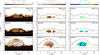 |
Fig. 8. Various components that determine the drift velocity uamb, calculated for Experiment 2. Left column: ratio |B|2/ρ2. Middle column: maps of |
The middle term of Eq. (14),  , is shown in the central column of Fig. 8. In the figure, one can see that the term is larger in the core of the dome than in the periphery during almost the whole evolution of the emerged dome, in fact by at least a few orders of magnitude. The reason for this is that the core of the dome is much less ionized than its periphery and, as already said, that term follows approximately the ratio ρn/ρi.
The two factors studied so far, when combined, give the value of the ambipolar diffusion coefficient. From the results just explained, one would expect ηamb to be larger toward the core of the dome and decreasing toward the periphery at the top and sides. This is indeed the case, as shown through the solid solid isocontours in the left and middle columns of Fig. 8, which correspond to ηamb = 1013 cm2 s−1 (green) and ηamb = 1015 cm2 s−1 (blue). Through those isocontours, we can also see that ηamb increases as the dome develops, specially in the innermost part. Therefore, during the first stages of the emergence, obtaining magnetic field slippage is less probable; in later stages, if any slippage occurs, it is likely to be located in the core of the emerged region.
Concerning the characteristic length of the magnetic field, our emerged regions are not simple idealized symmetric magnetic domes. This leads to a large complexity in the magnetic field structure that emerges. In order to show this, in the right column of Fig. 8, we have plotted  only in regions where the ambipolar diffusion coefficient is ηamb > 1013 cm2 s−1. In those panels, it is possible to find regions with variations in
  up to a few orders of magnitude, consequently meaning large variations in the module of the drift velocity uamb.
Additionally to the module, we can analyze the direction of uamb, given by the vector product  . For compactness, in the left and middle columns of Fig. 8 we have superimposed a set of red arrows to show the uamb vector field in regions where ηamb > 1013 cm2 s−1. The arrows do not show a clear pattern; sometimes even showing opposite directions in the velocity drift. In addition, in the accompanying movie, we find rapid variations of those directions, which reflects the highly dynamic environment of the emerged regions.
Once we know the dependencies of the module and direction of uamb, the next step is to analyze how large this drift velocity is in comparison with the plasma velocity u. To that end, the ratio |u|/|uamb| contained in the XZ-plane is studied. Figure 9 contains the results for the NEQ+AD branch of Experiment 2. The first thing we notice is that this ratio is only equal or smaller than 1 in some particular regions and that their corresponding area is smaller than the surface of the magnetized dome. In the accompanying animation of Fig. 9, we find that the regions where |uamb| dominates change faster than the characteristic times of the dome expansion; those regions also show rapid variations of the direction of uamb (red arrows). This means that the regions where field slippage could appear are small, and show rapid variations of the drift velocity in module and direction. As a consequence, no significant slippage (and therefore plasma material leakage) is found in our numerical experiments.
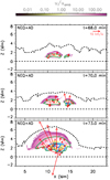 |
Fig. 9. Maps of |u|/|uamb| in the plane XZ. Two isocontours for ηamb are superimposed in the left and right column panels as green lines (1013 cm2 s−1) and blue lines (1015 cm2 s−1). The velocity field due to the ambipolar diffusion uamb (see Eq. (14)) is also shown in those columns with red arrows only in regions where ηamb > 1013 cm2 s−1. Additionally, dashed lines indicate the location of the solar surface (line at z = 0 Mm) and of the transition region (isocontour at T = 105 K). An animation of this figure is available online. |
4. Conclusions and discussion
We have performed two 2.5D radiative-MHD numerical experiments of magnetic flux emergence from the upper layers of the convection zone to the corona. The experiments were carried out using the Bifrost code, including an extra module that computes the NEQ formation of atomic and molecular hydrogen and another one that considers the partial ionization effects, in particular, the ambipolar diffusion. The time evolution of all the experiments leads to the formation of emerged magnetized regions with shapes similar to domes. The relevance of the NEQ and ambipolar diffusion effects were studied within those emerged domes as well as the role of H2 molecules and shocks in the thermodynamics of the magnetized domes. Furthermore, we have compared the amount of unsigned magnetic flux that emerges when including the NEQ ionization and recombination and ambipolar diffusion effects or otherwise. In the following, we summarize the main conclusions about the effects of the NEQ ionization and recombination and ambipolar diffusion when dealing with magnetic flux emergence, as well as some possible implications for other chromospheric environments.
In Sect. 3.1, it was shown that the LTE assumption can lead to an important underestimation of the ionization fraction in the emerged region, specially in the upper part where the difference can be up to 2−3 orders of magnitude. This has direct consequences on the ambipolar diffusion term since it inversely depends on the number of ions: assuming LTE can highly overestimate the effects of the ambipolar diffusion. The consequences of the NEQ ionization and recombination of hydrogen for the ambipolar diffusion may also have an impact on other chromospheric contexts, so one should be careful about the results that have been obtained under the LTE assumption.
This work shows that the formation rate of the H2 molecule is key in the thermodynamics of the emerged region. Under the LTE assumption, we find around 60−80% of H2 molecules by number within the emerged domes, while for the NEQ cases the maximum value is around 27%. The right determination of the number of H2 molecules is important to properly calculate their contribution to the energy due to their exothermic formation. Through observations, estimations of the fraction of H2 have been inferred in various sunspot umbrae using the equivalent width of the OH 15652 Å line as a proxy (Jaeggli et al. 2012); they find that substantial H2 molecule formation is present. However, the question remains open whether it would be possible to get similar estimates from observations of magnetic flux emergence regions.
The NEQ+AD branch of our two experiments shows that the strong cooling due to the expansion of the magnetized plasma during the emerging process can not be totally counteracted by the ambipolar diffusion heating. Consequently, artificial heating is still necessary to prevent even cooler temperatures than our threshold at 1660 K, where the radiation and EOS tables of the code are not accurate. The minimum temperature reached in flux emergence processes thus remains an open question and adds to the question of the minimum temperature in the quiet sun discussed by Leenaarts et al. (2011).
In Sect. 3.2, we could see that the emerged region is continually traversed by multiple shocks that have a significant impact on the thermodynamics of the magnetized domes. In particular, when considering the ambipolar diffusion in the NEQ branch, the temperature is up to a factor two greater than without ambipolar diffusion, while the ionization fraction can be up to one order of magnitude greater. The reason is the efficiency of the heating by ambipolar diffusion in the shocks, with characteristic times that range from 0.1 to 100 s. This heating mechanism can help to offset some of the strong cooling during the expansion of the emerging magnetized plasma. In this vein, by means of non-LTE inversions of observations, Leenaarts et al. (2018) have found evidences of heating in the chromosphere associated with flux emergence. The authors conjecture two possible sources for this heating: one associated with current sheets and a more homogeneous one due to ambipolar diffusion. However, those authors do not mention shocks as a possible source and we have not found homogeneous heating by ion-neutral collisions.
In Sect. 3.3, we analyzed in detail the effects of the ambipolar diffusion on the amount of emerged magnetic flux and lifted mass. We found that during the first stages after the buoyancy instability, mutual slippage of plasma and magnetic field is unlikely to take place due to the small values of the ambipolar diffusion coefficient, and therefore of the velocity drift of the ions. Later, the ambipolar diffusion increases, specially in the innermost part of the dome, and so does the velocity drift, as a consequence of the creation of more neutrals during the expansion of the magnetized plasma. However, the direction of the drift speed changes rapidly. On top of that, the regions where the drift can be important are a small fraction of the total area covered by the new magnetic flux and they are non-stationary. Consequently, the ambipolar diffusion does not significantly change the amount of emerged magnetic flux (as seen in Fig. 7 and Table 2), nor, consequently the amount of lifted mass, irrespective of the assumption of equilibrium equilibrium (NEQ or LTE). We have compared this result with the related ones in the literature. For instance, Leake & Arber (2006) found that the rate of magnetic flux emergence is considerably increased when including ambipolar diffusion in the calculation. Arber et al. (2007) found that the main difference between fully ionized 3D calculations and partially ionized ones is that the former are able to lift more chromospheric plasma. More recently, Leake & Linton (2013) improved the EOS used in the two previous papers by including changes in the internal energy density due to ionization and recombination. They showed that this change in the EOS significantly decreases the amount of out-of-plane magnetic flux (or shear flux) and mass lifted during the flux emergence process as compared to results with the previous EOS; however, they still find that simulations without ambipolar diffusion raise between 7.7 and 10 times more mass. We think that the main reason for the discrepancy with our results comes from the difference between the EOS. Those authors consider a plasma consisting of pure hydrogen. This means that as the temperature drops, the number of ions tends to zero due to the lack of other ionized elements that also contribute with electrons, resulting in large values of the ambipolar diffusion because  . In addition, those authors do not include the H2 molecule formation, so they do not have the pool of energy related to its exothermic formation that can also affect the thermodynamics. In order to show how important the choice of EOS is, Fig. 10 shows the ambipolar diffusion coefficient normalized to the magnetic field:

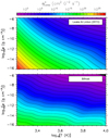 |
Fig. 10. Map of |


In the top panel of the figure,  is calculated as a function of density and temperature following the EOS used by Leake & Linton (2013); in the bottom panel, following the Bifrost EOS used for the LTE branches of this paper. The figure clearly shows that considering only hydrogen can lead to a substantial overestimate of the role of the ambipolar diffusion.
Through the results of this paper, we conclude that the NEQ imbalance in the populations of hydrogen together with ambipolar diffusion effects have important consequences for the dynamics and thermodynamics of magnetic flux emergence processes. Future research must explore the consequences of NEQ ionization and recombination in the ion populations of other elements. Also, further effects, like the Hall term in the generalized Ohm’s law, must be studied.
Movies
Movie of Fig. 2 Access here
Movie of Fig. 3 Access here
Movie of Fig. 4 Access here
Movie of Fig. 5 Access here
Movie of Fig. 8 Access here
Movie of Fig. 9 Access here
Movie of Fig. A.1 Access here
Acknowledgments
This research is supported by the Research Council of Norway through its Centres of Excellence scheme, project number 262622, and through grants of computing time from the Programme for Supercomputing. It is also supported by the Spanish Ministry of Science, Innovation and Universities through projects AYA2014-55078-P and PGC2018-095832-B-I00, as well as through the Synergy Grant number 810218 (ERC-2018-SyG) of the European Research Council; by NASA through grants NNX16AG90G, NNX17AD33G, 80NSSC18K1285 and contract NNG09FA40C (IRIS) and by the NSF grant AST1714955. The authors thankfully acknowledge the computer resources provided at the Pleiades cluster through the computing projects s1061, s1630, and s2053 from the High End Computing (HEC) division of NASA. In addition, this study has been discussed within the activities of team 399 “Studying magnetic-field-regulated heating in the solar chromosphere” at the International Space Science Institute (ISSI) in Switzerland.
References
- Alexiades, V., Amiez, G., & Gremaud, P.-A. 1996, Commun. Numer. Meth. Eng., 12, 31 [Google Scholar]
- Arber, T. D., Haynes, M., & Leake, J. E. 2007, ApJ, 666, 541 [NASA ADS] [CrossRef] [Google Scholar]
- Archontis, A., Moreno-Insertis, F., Galsgaard, K., Hood, A., & O’Shea, E. 2004, A&A, 426, 1047 [NASA ADS] [CrossRef] [EDP Sciences] [Google Scholar]
- Ballester, J. L., Alexeev, I., Collados, M., et al. 2018, Space Sci. Rev., 214, 58 [NASA ADS] [CrossRef] [Google Scholar]
- Bradshaw, S. J., & Cargill, P. J. 2006, A&A, 458, 987 [NASA ADS] [CrossRef] [EDP Sciences] [Google Scholar]
- Bradshaw, S. J., & Klimchuk, J. A. 2011, ApJS, 194, 26 [NASA ADS] [CrossRef] [Google Scholar]
- Bradshaw, S. J., & Mason, H. E. 2003, A&A, 401, 699 [NASA ADS] [CrossRef] [EDP Sciences] [Google Scholar]
- Braginskii, S. I. 1965, Rev. Plasma Phys., 1, 205 [Google Scholar]
- Cally, P. S., & Khomenko, E. 2018, ApJ, 856, 20 [NASA ADS] [CrossRef] [Google Scholar]
- Carlsson, M., & Leenaarts, J. 2012, A&A, 539, A39 [NASA ADS] [CrossRef] [EDP Sciences] [Google Scholar]
- Carlsson, M., & Stein, R. F. 1992, ApJ, 397, L59 [NASA ADS] [CrossRef] [Google Scholar]
- Carlsson, M., & Stein, R. F. 2002, ApJ, 572, 626 [NASA ADS] [CrossRef] [Google Scholar]
- Cheung, M. C. M., & Cameron, R. H. 2012, ApJ, 750, 6 [NASA ADS] [CrossRef] [Google Scholar]
- Cheung, M. C. M., & Isobe, H. 2014, Liv. Rev. Sol. Phys., 11, 3 [Google Scholar]
- Cheung, M. C. M., Schüssler, M., & Moreno-Insertis, F. 2007, A&A, 467, 703 [NASA ADS] [CrossRef] [EDP Sciences] [Google Scholar]
- Courant, R., Friedrichs, K., & Lewy, H. 1928, Math. Ann., 100, 32 [NASA ADS] [CrossRef] [MathSciNet] [Google Scholar]
- Cowling, T. G. 1976, Magnetohydrodynamics (Crane Russak and Co) [Google Scholar]
- De Pontieu, B., Martens, P. C. H., & Hudson, H. S. 2001, ApJ, 558, 859 [NASA ADS] [CrossRef] [Google Scholar]
- De Pontieu, B., McIntosh, S., Martinez-Sykora, J., Peter, H., & Pereira, T. M. D. 2015, ApJ, 799, L12 [NASA ADS] [CrossRef] [Google Scholar]
- Emonet, T., & Moreno-Insertis, F. 1998, ApJ, 492, 804 [NASA ADS] [CrossRef] [Google Scholar]
- Fan, Y. 2001, ApJ, 554, L111 [NASA ADS] [CrossRef] [Google Scholar]
- Fang, F., Fan, Y., & McIntosh, S. W. 2014, ApJ, 789, L19 [NASA ADS] [CrossRef] [Google Scholar]
- Forbes, T. G., & Priest, E. R. 1984, Sol. Phys., 94, 315 [NASA ADS] [CrossRef] [Google Scholar]
- Golding, T. P., Carlsson, M., & Leenaarts, J. 2014, ApJ, 784, 30 [NASA ADS] [CrossRef] [Google Scholar]
- Golding, T. P., Leenaarts, J., & Carlsson, M. 2016, ApJ, 817, 125 [NASA ADS] [CrossRef] [Google Scholar]
- González-Morales, P. A., Khomenko, E., Downes, T. P., & de Vicente, A. 2018, A&A, 615, A67 [NASA ADS] [CrossRef] [EDP Sciences] [Google Scholar]
- Goodman, M. L. 2000, ApJ, 533, 501 [NASA ADS] [CrossRef] [Google Scholar]
- Gudiksen, B. V., Carlsson, M., Hansteen, V. H., et al. 2011, A&A, 531, A154 [NASA ADS] [CrossRef] [EDP Sciences] [Google Scholar]
- Hansteen, V. 1993, ApJ, 402, 741 [NASA ADS] [CrossRef] [Google Scholar]
- Hansteen, V. H., Archontis, V., Pereira, T. M. D., et al. 2017, ApJ, 839, 22 [NASA ADS] [CrossRef] [Google Scholar]
- Hansteen, V., Ortiz, A., Archontis, V., et al. 2019, A&A, 626, A33 [NASA ADS] [CrossRef] [EDP Sciences] [Google Scholar]
- Hayek, W., Asplund, M., Carlsson, M., et al. 2010, A&A, 517, A49 [NASA ADS] [CrossRef] [EDP Sciences] [Google Scholar]
- Jaeggli, S. A., Lin, H., & Uitenbroek, H. 2012, ApJ, 745, 133 [NASA ADS] [CrossRef] [Google Scholar]
- Karlický, M., Bárta, M., & Rybák, J. 2010, A&A, 514, A28 [NASA ADS] [CrossRef] [EDP Sciences] [Google Scholar]
- Khomenko, E., & Cally, P. S. 2019, ApJ, 883, 179 [NASA ADS] [CrossRef] [Google Scholar]
- Khomenko, E., & Collados, M. 2012, ApJ, 747, 87 [NASA ADS] [CrossRef] [Google Scholar]
- Khomenko, E., Díaz, A., de Vicente, A., Collados, M., & Luna, M. 2014, A&A, 565, A45 [NASA ADS] [CrossRef] [EDP Sciences] [Google Scholar]
- Klein, R. I., Stein, R. F., & Kalkofen, W. 1976, ApJ, 205, 499 [NASA ADS] [CrossRef] [Google Scholar]
- Klein, R. I., Stein, R. F., & Kalkofen, W. 1978, ApJ, 220, 1024 [NASA ADS] [CrossRef] [EDP Sciences] [Google Scholar]
- Kneer, F. 1980, A&A, 87, 229 [NASA ADS] [Google Scholar]
- Krstic, P. S., & Schultz, D. R. 1999, J. Phys. B At. Mol. Phys., 32, 2415 [NASA ADS] [CrossRef] [Google Scholar]
- Leake, J. E., & Arber, T. D. 2006, A&A, 450, 805 [NASA ADS] [CrossRef] [EDP Sciences] [Google Scholar]
- Leake, J. E., & Linton, M. G. 2013, ApJ, 764, 54 [NASA ADS] [CrossRef] [Google Scholar]
- Leake, J. E., Arber, T. D., & Khodachenko, M. L. 2005, A&A, 442, 1091 [NASA ADS] [CrossRef] [EDP Sciences] [Google Scholar]
- Leenaarts, J., & Wedemeyer-Böhm, S. 2006, A&A, 460, 301 [NASA ADS] [CrossRef] [EDP Sciences] [Google Scholar]
- Leenaarts, J., Carlsson, M., Hansteen, V., & Rutten, R. J. 2007, A&A, 473, 625 [NASA ADS] [CrossRef] [EDP Sciences] [Google Scholar]
- Leenaarts, J., Carlsson, M., Hansteen, V., & Gudiksen, B. V. 2011, A&A, 530, A124 [NASA ADS] [CrossRef] [EDP Sciences] [Google Scholar]
- Leenaarts, J., de la Cruz Rodríguez, J., Danilovic, S., Scharmer, G., & Carlsson, M. 2018, A&A, 612, A28 [NASA ADS] [CrossRef] [EDP Sciences] [Google Scholar]
- Longcope, D. W., Fischer, G. H., & Arendt, S. 1996, ApJ, 464, 999 [NASA ADS] [CrossRef] [Google Scholar]
- MacTaggart, D., Guglielmino, S. L., Haynes, A. L., Simitev, R., & Zuccarello, F. 2015, A&A, 576, A4 [NASA ADS] [CrossRef] [EDP Sciences] [Google Scholar]
- Martínez-Sykora, J., Hansteen, V., & Carlsson, M. 2008, ApJ, 679, 871 [NASA ADS] [CrossRef] [Google Scholar]
- Martínez-Sykora, J., De Pontieu, B., & Hansteen, V. 2012, ApJ, 753, 161 [NASA ADS] [CrossRef] [Google Scholar]
- Martínez-Sykora, J., Moreno-Insertis, F., & Cheung, M. C. M. 2015a, ApJ, 814, 2 [NASA ADS] [CrossRef] [Google Scholar]
- Martínez-Sykora, J., De Pontieu, B., Hansteen, V., & Carlsson, M. 2015b, Roy. Soc. London Philos. Trans. Ser. A, 373, 40268 [NASA ADS] [CrossRef] [Google Scholar]
- Martínez-Sykora, J., De Pontieu, B., Carlsson, M., & Hansteen, V. 2016a, ApJ, 831, L1 [NASA ADS] [CrossRef] [Google Scholar]
- Martínez-Sykora, J., De Pontieu, B., Hansteen, V. H., & Gudiksen, B. 2016b, ApJ, 817, 46 [NASA ADS] [CrossRef] [Google Scholar]
- Martínez-Sykora, J., De Pontieu, B., Hansteen, V. H., et al. 2017a, Science, 356, 1269 [NASA ADS] [CrossRef] [Google Scholar]
- Martínez-Sykora, J., De Pontieu, B., Carlsson, M., et al. 2017b, ApJ, 847, 36 [NASA ADS] [CrossRef] [Google Scholar]
- Mitchner, M., & Kruger, C. H. 1973, Partially Ionized Gases (New York: John Wiley and Sons Inc) [Google Scholar]
- Moreno-Insertis, F. 2006, in Solar MHD Theory and Observations: A High Spatial Resolution Perspective, eds. J. Leibacher, R. F. Stein, & H. Uitenbroek, ASP Conf. Ser., 354, 183 [NASA ADS] [Google Scholar]
- Moreno-Insertis, F., & Emonet, T. 1996, ApJ, 472, L53 [NASA ADS] [CrossRef] [Google Scholar]
- Moreno-Insertis, F., & Galsgaard, K. 2013, ApJ, 771, 20 [NASA ADS] [CrossRef] [Google Scholar]
- Moreno-Insertis, F., Martínez-Sykora, J., Hansteen, V. H., & Muñoz, D. 2018, ApJ, submitted [Google Scholar]
- Newcomb, W. A. 1961, Phys. Fluids, 4, 391 [NASA ADS] [CrossRef] [MathSciNet] [Google Scholar]
- Ni, L., Zhang, Q.-M., Murphy, N. A., & Lin, J. 2017, ApJ, 841, 27 [NASA ADS] [CrossRef] [Google Scholar]
- Nóbrega-Siverio, D., Moreno-Insertis, F., & Martínez-Sykora, J. 2016, ApJ, 822, 18 [NASA ADS] [CrossRef] [Google Scholar]
- Nóbrega-Siverio, D., Martínez-Sykora, J., Moreno-Insertis, F., & Rouppe van der Voort, L. 2017, ApJ, 850, 153 [NASA ADS] [CrossRef] [Google Scholar]
- Nóbrega-Siverio, D., Moreno-Insertis, F., & Martínez-Sykora, J. 2018, ApJ, 858, 8 [NASA ADS] [CrossRef] [Google Scholar]
- Olluri, K., Gudiksen, B. V., & Hansteen, V. H. 2013, ApJ, 767, 43 [NASA ADS] [CrossRef] [Google Scholar]
- Olluri, K., Gudiksen, B. V., Hansteen, V. H., & De Pontieu, B. 2015, ApJ, 802, 5 [NASA ADS] [CrossRef] [Google Scholar]
- O’Sullivan, S., & Downes, T. P. 2007, MNRAS, 376, 1648 [NASA ADS] [CrossRef] [Google Scholar]
- Priest, E. 2014, Magnetohydrodynamics of the Sun (Cambridge: Cambridge University Press) [Google Scholar]
- Priest, E. R., & Forbes, T. G. 2002, A&ARv, 10, 313 [NASA ADS] [CrossRef] [Google Scholar]
- Raouafi, N. E., Patsourakos, S., Pariat, E., et al. 2016, Space Sci. Rev., 201, 1 [NASA ADS] [CrossRef] [Google Scholar]
- Reep, J. W., Warren, H. P., Crump, N. A., & Simões, P. J. A. 2016, ApJ, 827, 145 [NASA ADS] [CrossRef] [Google Scholar]
- Reep, J. W., Russell, A. J. B., Tarr, L. A., & Leake, J. E. 2018, ApJ, 853, 101 [NASA ADS] [CrossRef] [Google Scholar]
- Ruderman, M. S., Ballai, I., Khomenko, E., & Collados, M. 2018, A&A, 609, A23 [NASA ADS] [CrossRef] [EDP Sciences] [Google Scholar]
- Shelyag, S., Khomenko, E., de Vicente, A., & Przybylski, D. 2016, ApJ, 819, L11 [NASA ADS] [CrossRef] [Google Scholar]
- Shibata, K., Nozawa, S., & Matsumoto, R. 1992, PASJ, 44, 265 [NASA ADS] [Google Scholar]
- Skartlien, R. 2000, ApJ, 536, 465 [NASA ADS] [CrossRef] [Google Scholar]
- Soler, R., Carbonell, M., & Ballester, J. L. 2015, ApJ, 810, 146 [NASA ADS] [CrossRef] [Google Scholar]
- Tortosa-Andreu, A., & Moreno-Insertis, F. 2009, A&A, 507, 949 [NASA ADS] [CrossRef] [EDP Sciences] [Google Scholar]
- Vranjes, J., & Krstic, P. S. 2013, A&A, 554, A22 [NASA ADS] [CrossRef] [EDP Sciences] [Google Scholar]
- Vranjes, J., Poedts, S., Pandey, B. P., & de Pontieu, B. 2008, A&A, 478, 553 [NASA ADS] [CrossRef] [EDP Sciences] [Google Scholar]
- Yang, L., Peter, H., He, J., et al. 2018, ApJ, 852, 16 [Google Scholar]
- Yokoyama, T., & Shibata, K. 1995, Nature, 375, 42 [NASA ADS] [CrossRef] [Google Scholar]
- Yokoyama, T., & Shibata, K. 1996, PASJ, 48, 353 [NASA ADS] [CrossRef] [Google Scholar]
- Zhao, T.-L., Ni, L., Lin, J., & Ziegler, U. 2018, Res. Astron. Astrophys., 18, 045 [NASA ADS] [CrossRef] [Google Scholar]
- Zwaan, C. 1987, ARA&A, 25, 83 [NASA ADS] [CrossRef] [Google Scholar]
- Zweibel, E. G. 2015, in Magnetic Fields in Diffuse Media, eds. A. Lazarian, E. M. de Gouveia Dal Pino, & C. Melioli, Astrophys. Space Sci. Lib., 407, 285 [NASA ADS] [Google Scholar]
- Zweibel, E. G., Lawrence, E., Yoo, J., et al. 2011, Phys. Plasmas, 18, 111211 [NASA ADS] [CrossRef] [Google Scholar]
Appendix A: Choosing the instant to create the branches
One of the concerns when carrying out the present work was choosing the right instant to create the different branches. In this appendix, we prove that the NEQ and AD effects are negligible within the emerging magnetized plasma in the instants prior to our branching at t = 60 min, meaning that the results presented in this paper are not affected by our choice.
Concerning the NEQ effects, we compare the ion density in the NEQ+AD branch, ρi, with the ion density obtained from an LTE calculation based on the values of that experiment,  , using the following relative difference:

This ratio is shown for Experiments 1 and 2 at t = 60 min in the two uppermost panels of Fig. A.1, and from t = 50 to t = 60 min in the associated movie. In both panels, the location of the new emerging magnetic field is shown through a solid isocontour at |B| = 10 G in orange color. The values of ri clearly indicate that the departures in the ion density from ionization equilibrium occur higher up in the atmosphere and that t = 60 min is a safe point in which we can turn off the NEQ module without having already affected the emergence of the tube.
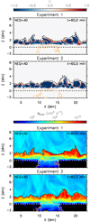 |
Fig. A.1. Maps of ri (see Eq. (A.1)) and ηamb for Experiments 1 and 2 at t = 60 min. The location of the new emerging magnetic field is shown through a solid isocontour at |B| = 10 G in orange color. Additionally, dashed lines indicate the location of the solar surface (line at z = 0 Mm) and of the transition region (isocontour at T = 105 K). An animation of this figure showing the evolution from t = 50 to t = 60 min is available online. |
Regarding the AD effects, we have plotted the ambipolar diffusion coefficient for Experiments 1 and 2 at t = 60 min in the two lowermost panels of Fig. A.1. As in the previous panels, the location of the new emerging magnetic field is shown by means of a solid isocontour at |B| = 10 G in orange color. During most of the emergence through the convection zone (see associated animation), the coefficient ηamb in the twisted tube is ≤102 cm2 s−1, which is smaller or comparable to the negligible values found in the corona. As the magnetized plasma reaches the surface and piles up, there is an increase in the ambipolar diffusion coefficient up to values around 105 − 106 cm2 s−1. These values are still 8−9 orders of magnitude smaller than the values we find later within the emerged region once it reaches the chromosphere and expands. As a consequence, we can create the branches without AD also at t = 60 min without having already affected the emergence of the tube.
All Tables
Scheme of the time evolution for the two experiments and the physical mechanisms included at the different stages.
All Figures
|
Fig. 1. Properties of the initial snapshot (t = 0 min). Panel A: horizontal averages of the initial stratification for temperature T (green), magnetic field strength B (black), pressure P (blue) and density ρ (red) normalized to their photospheric values at z = 0 Mm (Tph = 5803 K, Bph = 0.44 G, Pph = 1.12 × 10⁵ erg cm−3, and ρph = 3.20 × 10⁻⁷ g cm−3). The dotted vertical line delineates the solar surface. Panel B: 2D map for the initial background stratification of the temperature only showing values below T = 3 × 10⁴ K. The solar surface is roughly at z = 0 Mm (dashed horizontal black line). The other dashed line is an isocontour that delimits the transition region at T = 105 K. |
| In the text | |
|
Fig. 2. Emerged region for Experiment 1. The rows contain the four branches of this experiment, namely, in descending order, LTE, LTE+AD, NEQ, NEQ+AD. From left to right columns: ionization fraction, ρi/ρ; the temperature, T; and the fraction of molecular hydrogen, fH2. Dashed lines indicate the location of the solar surface (line at z = 0 Mm) and of the transition region (isocontour at T = 105 K). Solid white isocontours delimit the temperature threshold limit at T = 1660 K. An animation of this figure is available online. |
| In the text | |
|
Fig. 3. Emerged region for Experiment 2. The rows contain the four branches of this experiment, namely, in descending order, LTE, LTE+AD, NEQ, NEQ+AD. From left to right columns: ionization fraction, ρi/ρ; the temperature, T; and the fraction of molecular hydrogen, fH2. Dashed lines indicate the location of the solar surface (line at z = 0 Mm) and of the transition region (isocontour at T = 105 K). Solid white isocontours delimit the temperature threshold limit at T = 1660 K. An animation of this figure is available online. |
| In the text | |
|
Fig. 4. Divergence of the plasma velocity field, ∇ ⋅ u, for Experiments 1 (top) and 2 (bottom) at different stages of the magnetic flux emergence process. Arrows are superimposed pointing out the location of some of the shocks within the emerged regions. Dashed lines indicate the location of the solar surface (line at z = 0 Mm) and of the transition region (isocontour at T = 105 K). An animation of this figure is available online. |
| In the text | |
|
Fig. 5. Shock evolution within the emerged region for the Experiment 2 at different instants (rows). Left column: temperature, T, for the NEQ branch; middle column: T for the NEQ+AD case; and right column: characteristic time of the heating due to ambipolar diffusion, τqamb (see Eq. (9)). In addition, a solid line nearly perpendicular to the shock front has been superimposed in all the panels to study the variation of different quantities due to the shock passage (see Fig. 6). In the image, dashed lines indicate the location of the solar surface (line at z = 0 Mm) and of the transition region (isocontour at T = 105 K). An animation of this figure is available online. |
| In the text | |
|
Fig. 6. Evolution of different quantities along the cut plotted in Fig. 5 for the same instants reproduced in that image. The x and z coordinates along that line are given as abscissas in the bottom and top axes, respectively. Left panels: evolution of the temperature T (black lines, left axis) and ionization fraction ρi/ρ (blue lines, right axis) for the NEQ case (long dashed lines) and NEQ+AD (solid ones). Right panels: zoom of the gray region of the left panels. The curves are for the temperature (black), and the characteristic times τcomp (blue) and τqamb (orange), keeping the long dashed lines for the purely NEQ case and solid lines for the NEQ + AD one. The tick-marks for the temperature are given on the left axis, and those for the times on the right axis. For all panels, the threshold temperature, T = 1660 K, is shown with a horizontal dash-dotted line in red. |
| In the text | |
|
Fig. 7. Unsigned vertical flux Φ as a function of time during the flux emergence process for Experiment 1 (panels A and B) and Experiment 2 (panels C and D) for different heights, namely, z = [0.5,1.0,2.0,3.0,4.0,5.0] Mm. The LTE panel for each experiment contains |
| In the text | |
|
Fig. 8. Various components that determine the drift velocity uamb, calculated for Experiment 2. Left column: ratio |B|2/ρ2. Middle column: maps of |
| In the text | |
|
Fig. 9. Maps of |u|/|uamb| in the plane XZ. Two isocontours for ηamb are superimposed in the left and right column panels as green lines (1013 cm2 s−1) and blue lines (1015 cm2 s−1). The velocity field due to the ambipolar diffusion uamb (see Eq. (14)) is also shown in those columns with red arrows only in regions where ηamb > 1013 cm2 s−1. Additionally, dashed lines indicate the location of the solar surface (line at z = 0 Mm) and of the transition region (isocontour at T = 105 K). An animation of this figure is available online. |
| In the text | |
|
Fig. 10. Map of |
| In the text | |
|
Fig. A.1. Maps of ri (see Eq. (A.1)) and ηamb for Experiments 1 and 2 at t = 60 min. The location of the new emerging magnetic field is shown through a solid isocontour at |B| = 10 G in orange color. Additionally, dashed lines indicate the location of the solar surface (line at z = 0 Mm) and of the transition region (isocontour at T = 105 K). An animation of this figure showing the evolution from t = 50 to t = 60 min is available online. |
| In the text | |
Current usage metrics show cumulative count of Article Views (full-text article views including HTML views, PDF and ePub downloads, according to the available data) and Abstracts Views on Vision4Press platform.
Data correspond to usage on the plateform after 2015. The current usage metrics is available 48-96 hours after online publication and is updated daily on week days.
Initial download of the metrics may take a while.