The ISM scaling relations in DustPedia late-type galaxies: A benchmark study for the Local Universe

V. Casasola; S. Bianchi; P. De Vis; L. Magrini; E. Corbelli; C. J. R. Clark; J. Fritz; A. Nersesian; S. Viaene; M. Baes; L. P. Cassarà; J. Davies; I. De Looze; W. Dobbels; M. Galametz; F. Galliano; A. P. Jones; S. C. Madden; A. V. Mosenkov; A. Trčka; E. Xilouris

doi:10.1051/0004-6361/201936665

Home

All issues

Volume 633 (January 2020)

A&A, 633 (2020) A100

Full HTML

Free Access

Issue		A&A Volume 633, January 2020


Article Number		A100
Number of page(s)		20
Section		Extragalactic astronomy
DOI		https://doi.org/10.1051/0004-6361/201936665
Published online		20 January 2020

A&A 633, A100 (2020)

The ISM scaling relations in DustPedia late-type galaxies: A benchmark study for the Local Universe^⋆

V. Casasola¹^,2, S. Bianchi², P. De Vis³, L. Magrini², E. Corbelli², C. J. R. Clark⁴, J. Fritz⁵, A. Nersesian⁶^,7^,8, S. Viaene⁸, M. Baes⁸, L. P. Cassarà⁹^,6, J. Davies³, I. De Looze¹⁰^,8, W. Dobbels⁸, M. Galametz¹¹, F. Galliano¹¹, A. P. Jones¹², S. C. Madden¹¹, A. V. Mosenkov¹³^,14, A. Trčka⁸ and E. Xilouris⁶

¹ INAF – Istituto di Radioastronomia, Via P. Gobetti 101, 40129 Bologna, Italy
e-mail: viviana.casasola@inaf.it
² INAF – Osservatorio Astrofisico di Arcetri, Largo E. Fermi 5, 50125 Firenze, Italy
³ School of Physics and Astronomy, Cardiff University, The Parade, Cardiff CF24 3AA, UK
⁴ Space Telescope Science Institute, 3700 San Martin Drive, Baltimore, Maryland 21218, USA
⁵ Instituto de Radioastronomía y Astrofísica, UNAM, Campus Morelia, A.P. 3-72, Morelia 58089, Mexico
⁶ National Observatory of Athens, Institute for Astronomy, Astrophysics, Space Applications and Remote Sensing, Ioannou Metaxa and Vasileos Pavlou, 15236 Athens, Greece
⁷ Department of Astrophysics, Astronomy & Mechanics, Faculty of Physics, University of Athens, Panepistimiopolis, 15784 Zografos, Athens, Greece
⁸ Sterrenkundig Observatorium Universiteit Gent, Krijgslaan 281 S9, 9000 Gent, Belgium
⁹ INAF – Istituto di Astrofisica Spaziale e Fisica cosmica, Via A. Corti 12, 20133 Milano, Italy
¹⁰ Department of Physics and Astronomy, University College London, Gower Street, London WC1E 6BT, UK
¹¹ Laboratoire AIM, CEA/DSM – CNRS – Université Paris Diderot, IRFU/Service d’Astrophysique, CEA Saclay, 91191 Gif-sur-Yvette, France
¹² Institut d’Astrophysique Spatiale, CNRS, Univ. Paris-Sud, Université Paris-Saclay, Bât. 121, 91405 Orsay Cedex, France
¹³ Central Astronomical Observatory of RAS, Pulkovskoye Chaussee 65/1, 196140 St. Petersburg, Russia
¹⁴ St. Petersburg State University, Universitetskij Pr. 28, 198504 St. Petersburg, Stary Peterhof, Russia

Received: 10 September 2019
Accepted: 18 November 2019

Abstract

Aims. The purpose of this work is the characterization of the main scaling relations between all of the interstellar medium (ISM) components, namely dust, atomic, molecular, and total gas, and gas-phase metallicity, as well as other galaxy properties, such as stellar mass (M_star) and galaxy morphology, for late-type galaxies in the Local Universe.

Methods. This study was performed by extracting late-type galaxies from the entire DustPedia sample and by exploiting the large and homogeneous dataset available thanks to the DustPedia project. The sample consists of 436 galaxies with morphological stage spanning from T = 1−10, M_star from 6 × 10⁷ to 3 × 10¹¹ M_⊙, star formation rate from 6 × 10⁻⁴ to 60 M_⊙ yr⁻¹, and oxygen abundance from 12 + log(O/H) = 8−9.5. Molecular and atomic gas data were collected from the literature and properly homogenized. All the masses involved in our analysis refer to the values within the optical disks of galaxies. The scaling relations involving the molecular gas are studied by assuming both a constant and a metallicity-dependent CO-to-H₂ conversion factor (X_CO). The analysis was performed by means of the survival analysis technique, in order to properly take into account the presence of both detection and nondetection in the data.

Results. We confirm that the dust mass correlates very well with the total gas mass, and find –for the first time– that the dust mass correlates better with the atomic gas mass than with the molecular one. We characterize important mass ratios such as the gas fraction, the molecular-to-atomic gas mass ratio, the dust-to-total gas mass ratio (DGR), and the dust-to-stellar mass ratio, and study how they relate to each other, to galaxy morphology, and to gas-phase metallicity. Only the assumption of a metallicity-dependent X_CO reproduces the expected decrease of the DGR with increasing morphological stage and decreasing gas-phase metallicity, with a slope of about 1. The DGR, the gas-phase metallicity, and the dust-to-stellar mass ratio are, for our galaxy sample, directly linked to galaxy morphology. The molecular-to-atomic gas mass ratio and the DGR show a positive correlation for low molecular gas fractions, but for galaxies rich in molecular gas this trend breaks down. To our knowledge, this trend has never been found before, and provides new constraints for theoretical models of galaxy evolution and a reference for high-redshift studies. We discuss several scenarios related to this finding.

Conclusions. The DustPedia database of late-type galaxies is an extraordinary tool for the study of the ISM scaling relations, thanks to its homogeneous collection of data for the different ISM components. The database is made publicly available to the whole community.

Key words: galaxies: ISM / galaxies: evolution / dust / extinction / ISM: atoms / ISM: molecules / ISM: abundances

^⋆

DustPedia is a project funded by the EU under the heading “Exploitation of space science and exploration data”. It has the primary goal of exploiting existing data in the Herschel Space Observatory and Planck Telescope databases.

© ESO 2020

1. Introduction

The global properties of nearby galaxies are related by an intricate system of correlations that form the basis of the so-called “scaling relations”. They allow us to study the internal physics in different galaxy populations, as well as their formation and evolutionary histories.

Among the first recognized relationships, we recall the Tully-Fisher relation for spiral galaxies (Tully & Fisher 1977) and the Fundamental Plane for elliptical galaxies (Djorgovski & Davis 1987; Jorgensen et al. 1996). Thanks to the flowering of spectroscopic and photometric surveys of galaxies, recent decades have seen the elucidation of new relationships among galaxy properties, such as those between the star formation rate (SFR) and the stellar mass in galaxies, the so-called main sequence (MS) of star forming galaxies (e.g., Brinchmann et al. 2004; Daddi et al. 2007; Elbaz et al. 2007; Noeske et al. 2007; Santini et al. 2009, 2017; Peng et al. 2010; Rodighiero et al. 2014; Speagle et al. 2014; Whitaker et al. 2014; Schreiber et al. 2015; Tasca et al. 2015; Tomczak et al. 2016). Furthermore, relationships have been discovered between the stellar mass and the average oxygen abundance, the mass–metallicity (MZ) relation (e.g., Lequeux et al. 1979; Garnett & Shields 1987; Vila-Costas & Edmunds 1992; Tremonti et al. 2004; Erb et al. 2006; Erb 2008; Henry et al. 2013; Maier et al. 2014, 2015, 2016; Salim et al. 2015; Sánchez et al. 2017), and the Kennicutt-Schmidt (KS) star formation (SF) relation (Schmidt 1959, 1963; Kennicutt 1998a,b), relating SFR and the surface density of cold gas in disks. Both the MS and MZ have been confirmed at different redshifts, showing a change with cosmological time and thus tracing the evolution of galaxy properties with time (e.g., Davé et al. 2011).

In the last few years, the number of studies dedicated to scaling relations of the interstellar medium (ISM) components has also grown (e.g., Saintonge et al. 2011a,b; Catinella et al. 2012, 2013, 2018; Corbelli et al. 2012; Boselli et al. 2014; Cortese et al. 2011, 2012, 2016; Santini et al. 2014; De Vis et al. 2017a,b; Calette et al. 2018; Zuo et al. 2018; Cook et al. 2019; Ginolfi et al. 2019; Lin et al. 2019; Lisenfeld et al. 2019; Sorai et al. 2019; Yesuf & Ho 2019). These studies have quickly become references and offer constraints for cosmological models of galaxy evolution, which are able to trace the evolution of the different gas phases (e.g., Gnedin et al. 2009; Dutton 2009; Dutton & van den Bosch 2009; Fu et al. 2010; Power et al. 2010; Cook et al. 2010; Lagos et al. 2011a,b; Kauffmann et al. 2012; Bahé et al. 2016; Camps et al. 2016; Crain et al. 2017; Marinacci et al. 2017; Diemer et al. 2019; Stevens et al. 2019). However, in most of the previous studies the contribution of dust to the ISM was neglected. The mass of the ISM is indeed made up of ∼99% gas (∼74% of hydrogen, ∼25% of helium, and ∼1% of heavier elements, i.e., “metals”), and ∼1% dust. Although dust occupies a small percentage in the ISM mass budget, it is a key component, driving several processes in the ISM: by absorbing and scattering the ionizing and nonionizing light of the interstellar radiation field, dust participates in the energetic balance that regulates the heating and cooling process of the ISM (see e.g., Galliano et al. 2018, for a comprehensive overview of the interstellar dust in nearby galaxies). The formation of molecules in the ISM happens on the surface of dust grains which subsequently act as a screen to protect these molecules from dissociation. Dust also prevents the dissociation of molecules and favors gas fragmentation and the formation of stars (e.g., Scoville et al. 2013).

Dust radiates most of its energy as far-infrared (FIR) continuum emission. The Herschel satellite has played an important role in the study of dust thanks to its superior angular resolution and/or sensitivity compared to previous FIR space and ground-based facilities (e.g., IRAS, ISO, Spitzer, MAMBO, LABOCA); Herschel operates right across the peak of the dust spectral energy distribution (SED, 70 − 500 μm). This makes Herschel sensitive to the diffuse cold (T < 25 K) dust component that dominates the dust mass in galaxies (Devereux & Young 1990; Dunne & Eales 2001; Draine et al. 2007; Clark et al. 2015), as well as to warmer (T > 30 K) dust radiating at shorter wavelengths which often dominates the dust luminosity.

Making use of the Herschel data, the DustPedia project is definitively characterizing the dust properties in the Local Universe by exploiting a database of multi-wavelength imagery and photometry that greatly exceeds the scope (in terms of wavelength coverage and number of galaxies) of any similar survey (Clark et al. 2018). The original DustPedia sample consists of 875 extended (D₂₅ > 1′)¹ galaxies of all morphological types, within v = 3000 km s⁻¹ (z < 0.01), and observed by Herschel (see Davies et al. 2017, for a detailed description of the DustPedia sample).

In the present work, we select from the DustPedia database², a sample of nearby late-type galaxies to study the correlations between the various components of the ISM. We focus on late-type galaxies because they have – on average – a richer ISM content than early-type galaxies (e.g., Casasola et al. 2004; Cortese et al. 2012; Nersesian et al. 2019). In particular, more observational campaigns and single-object studies have been performed on the molecular gas content of late-type galaxies and with a higher detection rate than similar investigations in early-type galaxies (e.g., Combes et al. 2007; O’Sullivan et al. 2018; Espada et al. 2019). Our galaxy sample covers large dynamic ranges of various galactic physical properties: morphological stage 1 ≤ T ≤ 10, 10⁸ M_⊙ ≲ M_star ≲ 10¹¹ M_⊙, 10⁻³ M_⊙ yr⁻¹ ≲ SFR ≲ 60 M_⊙ yr⁻¹, and oxygen abundance 8.0 ≤ 12 + log(O/H) ≤ 9.5. These ranges exceed those of any similar studies making our sample ideal to investigate the ISM scaling relations.

All the derived quantities have been collected to obtain a homogeneous and statistically significant dataset. In particular, we estimate all the physical properties in a common region, namely within the optical disk of the galaxies. To our knowledge, this is a novel approach with respect to previous works: we compare different galactic properties in a very large sample of galaxies, but considering exactly the same regions within each galaxy. This allows us to produce consistent comparisons between masses of co-spatial galactic properties. In addition, DustPedia uses uniform prescriptions (i.e., models) to transform the observed quantities into dust and stellar masses (see later). Thus, our uniform treatment of data and modeling provides a complete and homogeneous galaxy sample able to put constraints on future cosmological hydro simulations predicting ISM properties and scaling relations and hopefully taking into account all ISM components. In this regard, we mention that an incoming DustPedia paper is focused on the comparison between DustPedia and EAGLE galaxies (Trčka et al. 2019).

The paper is organized as follows. In Sect. 2 we outline the sample selection and in Sect. 3 we present data used in this work, in particular the derivation of the masses and their distribution as a function of morphological type. In Sect. 4 we present and discuss scaling relations between the dust and atomic, molecular, and total gas masses, and also relations between stellar and gas masses. In Sect. 5 we study various mass ratios, also involving the stellar mass, as a function of different galaxy properties such as galaxy morphology and gas-phase metallicity. We highlight and summarize our main results in Sect. 6. In Appendices A and B, we collect the main properties of gas data and describe caveats and uncertainties associated with our analysis.

2. The galaxy sample

Our selection is based on the following criteria applied to the DustPedia database: (i) Hubble stage T ranging from 1 to 10; (ii) available global flux at 250 μm > 3σ; (iii) no significant contamination to the global flux from nearby galactic or extragalactic sources, and no images with artifacts or insufficient sky coverage for a proper estimate of the target/sky levels. The flux selection, required by the companion work of Bianchi et al. (2019), cuts about 20% of all late-type DustPedia galaxies, while the quality selection cuts only 5%. We further discuss the effect of the flux selection in Sect. 3.4. The selected sample is composed of 436 DustPedia late-type galaxies.

Our sample is divided into bins following the Hubble stage T. The morphology indicator T is obtained from the HyperLEDA database (Makarov et al. 2014) and it can be a noninteger since for most objects the final T is averaged over various estimates available in the literature. Following Bianchi et al. (2018), we use all objects in the range [T − 0.5, T + 0.5) to define a sample characterized by a given integer T (e.g., the Sa sample defined by T = 1 include all objects with 0.5 ≤ T < 1.5). We use distances and other galaxy properties (e.g., $r_{25}^{1}$ $r_{25}^{1}$ ) collected by Clark et al. (2018) and distributed together with the DustPedia photometry.

About 50% of sample galaxies are classified as interacting systems. This definition of interacting galaxies is very broad, including pair and group members and parents of a companion galaxy according to the NED homogenized classification. According to the NED classification, approximately 12% of sample galaxies are low-luminosity active galactic nuclei (AGNs, e.g., L_X < 10⁴² erg s⁻¹), including Seyferts and LINERs, and ∼2% are starbursts. Table 1 collects the number of galaxies in the main sample for each morphological type, with some interaction or activity of our sample galaxies.

Table 1.

Classification of the main properties of the DustPedia late-type galaxy sample.

As shown in the following section, most of the galaxies in the main sample have high-quality Herschel data (dust content). In addition, most of them have been observed at 21 cm, and therefore we know their total atomic gas content, and an estimate of their stellar mass is available. Moreover, for an important fraction of them, gas-phase metallicities and ¹²CO emission line data (and therefore molecular gas mass content) are available.

3. The data

For the present work, we collect from the literature observations of molecular (Sect. 3.1) and atomic gas (Sect. 3.2). We describe here the data homogenization process and the estimate of the gas masses within r₂₅. We use this aperture since it contains most of the dust (and stellar) luminosity (e.g., Pohlen et al. 2010; Casasola et al. 2017; Clark et al. 2018). We also use dust and stellar masses, and gas-phase metallicities as described in a companion work of the DustPedia collaboration (Sect. 3.3).

We stress that the dust and stellar fluxes of Clark et al. (2018) used to derive the corresponding masses of DustPedia galaxies can refer to radii beyond the optical disk. The aperture-fitting process of Clark et al. (2018) is indeed based on an elliptical aperture in every band for a given target, and these apertures are then combined to provide a final aperture for the target. This approach has provided consistent optical coverage for all DustPedia galaxies (see Clark et al. 2018, for more details), and the study focusing on DustPedia face-on spiral galaxies by Casasola et al. (2017) showed that the total dust and stellar masses are a good approximation of their values within the optical radius. Table 2 summarizes the data available for our galaxy sample.

Table 2.

Total data collected for the studied galaxy sample.

3.1. The molecular gas

For the molecular gas, we bring together ¹²CO observations from a wide variety of sources (see Table A.1). We use data on ¹²CO(1–0), ¹²CO(2–1), and ¹²CO(3–2) emission lines, observed at 2.6 mm (115 GHz), 1.3 mm (230 GHz), and 0.87 mm (345 GHz), respectively. For each galaxy, our first choice is the ¹²CO(1–0) emission line, when available and of high quality (e.g., high signal-to-noise ratio). The second choice is the ¹²CO(2–1) line, and the third and final choice is the ¹²CO(3–2) line. We report ¹²CO(2–1) and ¹²CO(3–2) emission lines to the ¹²CO(1–0) one by adopting the ¹²CO line ratios R₂₁ (=I₂₁/I₁₀), R₃₂ (=I₃₂/I₂₁), and R₃₁ (=I₃₂/I₁₀). When available, we use values measured for a given galaxy (e.g., NGC 1808, Aalto et al. 1994). Otherwise, we assume R₂₁ = 0.7, as determined in the HERACLES survey (Leroy et al. 2009, see also Casasola et al. 2015) and extensively used in studies of nearby late-type galaxies (e.g., Schruba et al. 2011; Casasola et al. 2017); and R₃₂ = 0.36 and R₃₁ = 0.18, determined by Wilson et al. (2012).

In most cases, observations are given in terms of different temperature scales (see Table A.2) which can be transformed into a common scale following Boselli et al. (2014) and the prescriptions of Kutner & Ulich (1981). We homogenize the dataset by transforming all temperatures into ¹²CO(1–0) fluxes, with S_CO in units of Jy km s⁻¹, following Table A.2. In two cases (NGC 3198 and NGC 3256), we extracted the H₂ mass (M_H₂) from the literature. These masses were properly transformed into the total ¹²CO flux, by adopting the distance and the CO-to-H₂ conversion factor used in the original reference.

3.1.1. Derivation of the ¹²CO flux within the optical disk

Most of our galaxies (∼92%) have single-beam ¹²CO observations usually pointed on the center of the galaxy and with a beam smaller than r₂₅. The ¹²CO flux must then be corrected for aperture effects to derive the total line flux. Since our sample contains highly inclined galaxies (i > 60°), we follow Boselli et al. (2014) and assume that the ¹²CO emission is well described by an exponential decline both along the radius and above the galactic plane:

$\begin{matrix} S_{CO} (r, z) = S_{CO} (0) e^{- r / r_{CO}} e^{- | z | / z_{CO}}, \end{matrix}$ $\begin{aligned} {S_{\rm CO}(r,z)} = S_{\rm CO}(0)\mathrm{e}^{-r/r_{\rm CO}}\mathrm{e}^{-|z|/z_{\rm CO}}, \end{aligned}$ (1)

with r_CO and z_CO being the scale-length and scale-height of the disk, respectively. For galaxies with low inclination, the method is analogous to the standard 2D approach, such as that developed by Lisenfeld et al. (2011). The method is based on the fact that the ¹²CO emission of nearby mapped galaxies can be described by an exponential disk: its radial scale-length r_CO correlates well with the optical scale-length of the stellar disk and with r₂₅ (Lisenfeld et al. 2011; Casasola et al. 2017). By assuming an average ratio r_CO/r₂₅, the ¹²CO 2D distribution can be simulated, convolved with the beam profile in order to scale it to the observation in the center of the galaxy, and finally integrated to obtain the total ¹²CO flux (e.g., Stark et al. 1986; Young et al. 1995; Corbelli et al. 2012). We assume here r_CO/r₂₅ = 0.17 ± 0.03, as derived by Casasola et al. (2017) for a sub-sample of DustPedia face-on spiral galaxies and consistent with the values of Leroy et al. (2008) and Lisenfeld et al. (2011). For galaxies closer to the edge-on case, the thickness of the disk must be taken into account: we use z_CO/r₂₅ = 1/100, defined by Boselli et al. (2014) from CO and dust emission models and observations of edge-on galaxies.

A few galaxies (∼4% of the sample) instead have angular sizes smaller than the ¹²CO beam. When not clearly specified in the original reference, we have corrected these ¹²CO data for beam dilution $T_{B} = T_{mb} (\frac{θ_{S}^{2} + θ_{beam}^{2}}{θ_{S}^{2}})$ $T_{\mathrm{B}} = T_{\mathrm{mb}} (\frac{\theta_{\mathrm{S}}^2 + \theta_{\mathrm{beam}}^2}{\theta_{\mathrm{S}}^2} )$ , where T_B is the brightness temperature and θ_S the source size.

3.1.2. CO-to-H₂ conversion and mass of H₂

The mass of molecular hydrogen M_H₂ is derived under the assumption of optically thick ¹²CO(1–0) emission, through the formula:

$\begin{matrix} M_{H_{2}} = 3.9 \times 10^{- 17} \times X_{CO} \times S_{CO} \times D^{2}, \end{matrix}$ $\begin{aligned} {M_{{\mathrm{H} }_2}} = 3.9 \times 10^{-17} \times X_{\rm CO} \times S_{\rm CO} \times D^2, \end{aligned}$ (2)

where M_H₂ is in units of M_⊙, S_CO is the ¹²CO(1–0) flux in units of Jy km s⁻¹, aperture-corrected as in Sect. 3.1.1, and D is the galaxy distance extracted from the DustPedia database in units of megaparsecs. The derivation of the total molecular mass in Eq. (2) requires knowledge of the CO-to-H₂ conversion factor, X_CO. We make two different assumptions on X_CO: (i) a constant value in agreement with the recommended value for Milky Way-like disks, which represents most galaxies of our sample, X_CO = 2.0 × 10²⁰ cm⁻² (K km s⁻¹)⁻¹ with ±30% uncertainty from Bolatto et al. (2013); and (ii) a metallicity-dependent X_CO as in Amorín et al. (2016). The study of these two assumptions on X_CO provides a conservative range of molecular gas mass estimations that demonstrates how uncertain the molecular gas mass derivation is.

As derived by observations (e.g., Bolatto et al. 2008, 2013; Casasola et al. 2007; Magrini et al. 2011; Accurso et al. 2017; Remy et al. 2017) and by theoretical models (e.g., Glover & Mac Low 2011; Narayanan et al. 2012; Gong et al. 2018), the X_CO conversion factor can vary due to effects of metallicity, gas temperature and abundance, optical depth, cloud structure, cosmic ray density, and ultraviolet radiation field. The dependence of X_CO on the abundance of the heavy elements is particularly debated in the literature: there are several relationships of X_CO with metallicity, showing a range of behaviors (e.g., Wilson 1995; Arimoto et al. 1996; Barone et al. 2000; Israel 2000; Boselli et al. 2002; Magrini et al. 2011; Schruba et al. 2012; Hunt et al. 2015a; Amorín et al. 2016). These relationships, although different, show a general increase of X_CO with decreasing metallicity. Particular attention is paid to galaxies with metallicity below ∼20% solar, such as blue compact dwarfs, for which very deep observational campaigns are needed to detect the ¹²CO(1–0) line (Madden et al. 2013; Cormier et al. 2014; Hunt et al. 2014, 2015a, 2017). Since the abundances in our sample are not particularly extreme (see Sect. 3.3), we adopted the metallicity-dependent CO-to-H₂ conversion factor by Amorín et al. (2016), which is derived combining low-metallicity starburst galaxies with more metal-rich galaxy objects, including the Milky Way and Local Volume galaxies from Leroy et al. (2011): X_CO ∝ (Z/Z_⊙)^−1.5 (see the fit in Fig. 11 of Amorín et al. 2016, where the conversion factor is given in terms of the equivalent α_CO [M_⊙ pc⁻² (K km s⁻¹)⁻¹] = 1.6 × 10⁻²⁰X_CO [cm⁻² (K km s⁻¹)⁻¹]). The power law of the calibration of Amorín et al. (2016) is also in qualitative agreement with previous determinations (e.g., Genzel et al. 2012; Schruba et al. 2012) and model predictions (e.g., Wolfire et al. 2010, as presented in Sandstrom et al. 2013).

Uncertainties in M_H₂ are calculated as the quadrature sum of the uncertainty on the ¹²CO(1–0) flux and on the X_CO conversion factor. Under the assumption of a metallicity-dependent X_CO, uncertainties in M_H₂ also take into account uncertainties on the metallicity and on the calibration of X_CO with the metallicity.

3.2. The atomic gas

De Vis et al. (2019) collected all available HI 21 cm emission line observations from the literature for the whole DustPedia sample. The HI fluxes S_HI are provided in units of Jy km s⁻¹; as for ¹²CO data, they come from various telescopes characterized by different beams. Table A.3 collects telescopes and beams of the HI data used in the current work. The mass of the atomic gas, M_HI, under the assumption of optically thin HI emission, is given by

$\begin{matrix} M_{HI} = 2.356 \times 10^{5} \times S_{HI} \times D^{2}, \end{matrix}$ $\begin{aligned} {M_{\rm HI}} = 2.356 \times 10^5 \times S_{\rm HI}\times D^2, \end{aligned}$ (3)

where M_HI is in units of M_⊙ and the distance D is in megaparsecs. Uncertainties in M_HI have been calculated from the uncertainty on the HI flux.

In highly inclined galaxies, HI emission might not be optically thin. Haynes & Giovanelli (1984) derived empirical corrections for galaxies of different axial ratios b/a and found that the HI flux could be underestimated by more than 20% for galaxies with b/a ≤ 0.25 and type Sc-Sd only. Our main sample contains only 12 such galaxies, a number that cannot alter the results of this study. We also find no significant overestimation of the dust-to-gas mass ratio for galaxies seen at edge-on inclinations (we have used the values derived by Mosenkov et al. 2019) if we use either HI only, or the total gas mass including the molecular phase. We therefore conclude that the assumption of the optically thin H I is valid and the HI masses used in this work are not severely underestimated.

Contrary to ¹²CO, HI observations typically cover a region similar to or larger than r₂₅ (compare the beam sizes in Tables A.2 and A.3). In particular, 77% of the available HI observations refer to larger sky areas. Therefore, before estimating the mass, it has been necessary to correct (i.e., reduce) S_HI to obtain the HI line flux within the optical radius.

We estimate the HI flux within r₂₅ adopting the model of the radial HI surface density profiles of Wang et al. (2014) obtained from azimuthally averaged radial profiles of HI gas in 42 galaxies from the Bluedisk sample (Wang et al. 2013). Their model for the HI profiles is an exponential function of radius in the outer regions with a depression towards the center, and it scales with R1³. In the outer regions, the radial HI surface density profiles are highly homogeneous for all galaxies, and exponentially declining parts have a scale-length of ∼0.18 R1 (see Fig. 10 in Wang et al. 2014). Similar results were found by Cayatte et al. (1994) and Martinsson et al. (2013), for example. Following Wang et al. (2014, see in particular their Eqs. (9) and (10)) and by integrating Σ_HI(r) up to r₂₅/R1, we derived the H I mass within r₂₅ for our galaxies with observations of larger extent. For these galaxies, the HI mass reduces by about ∼30–35%. The adopted method is preferred to other available methods (see, e.g., Bigiel & Blitz 2012) since it is applicable to almost the totality of our galaxy sample, it is based only on H I observations, and it is valid for both interacting and noninteracting galaxies.

It is important to stress that by focusing within the optical radius of late-type galaxies, the HI mass suffers the strongest reduction compared to the other ISM components and galaxy properties. It is also well known that the atomic gas beyond r₂₅ is very interesting. The need to derive HI mass within the common radius of r₂₅ is also dictated by the fact the original HI fluxes cover regions not only typically larger than r₂₅ but also larger than r₂₅ in a different way. Therefore, the choice of adopting the optical radius as size to explore scaling relations represents a solid normalization parameter. As already mentioned in Sect. 1, we are looking at different properties in a very large sample of galaxies, and always in exactly the same region of each galaxy. This is a novel approach with respect to those adopted in well-known surveys such as COLD GASS and xGASS (e.g., Saintonge et al. 2016; Catinella et al. 2018), where no restrictions were applied to fluxes used to derive the corresponding masses.

As typically done in similar studies, we assume that the total gas mass is the sum of the atomic and molecular gas masses, corrected for the helium contribution by multiplying by a factor of 1.36 (M_tot gas = 1.36 × [M_H₂ + M_HI]).

We refer to the subsample of galaxies that have detected molecular and atomic gas masses, as well as dust masses, as the gaseous sample; there are 202 galaxies in this sample (see Table 2).

3.3. Other DustPedia quantities

Dust masses (M_d) and stellar masses (M_star) of DustPedia galaxies were obtained through the modeling of their spectral energy distribution (SED). The Code Investigating GALaxy Evolution (CIGALE)⁴ was used (Boquien et al. 2019). CIGALE allows us to model the SED of a galaxy by choosing a variety of modules for the stellar, gas, and dust emission, and for dust attenuation (Noll et al. 2009; Roehlly et al. 2014; Boquien et al. 2019). In the version of CIGALE adopted by the DustPedia collaboration, the dust emission templates are computed from the DustPedia reference grain model (THEMIS⁵; Jones et al. 2017). For the full description of the DustPedia/CIGALE sample selection and modeling we refer to Nersesian et al. (2019; see also Bianchi et al. 2018).

The estimates and uncertainties of M_d and M_star from CIGALE are based on Bayesian statistics. Four galaxies of our sample (NGC 0253, NGC 4266, NGC 4594, NGC 7213) lack dust and stellar masses (see Table 2); they have not been fitted by CIGALE because their optical and mid-infrared (MIR) fluxes are contaminated or because of null coverage in the MIR and FIR bands.

Global oxygen abundances are available for a significant fraction of DustPedia galaxies (De Vis et al. 2019). As in most studies, we assume that the oxygen abundance is a good tracer of the total gas-phase metallicity. This assumption is justified by the fact that oxygen is the most abundant element besides H and He in the Universe. In addition, it is among the dominant constituents of dust (e.g., Savage & Sembach 1996; Jenkins 2009). We adopt a solar oxygen abundance of 12 + log(O/H) = 8.69 ± 0.05 from Asplund et al. (2009). The global metallicities provided by De Vis et al. (2019) are given at r = 0.4 × r₂₅ due to the statistically confirmed relationship between the luminosity-weighted integrated metallicity and the characteristic abundance (Kobulnicky et al. 1999; Pilyugin et al. 2004; Moustakas & Kennicutt 2006; Moustakas et al. 2010).

Among the available metallicity determinations in De Vis et al. (2019), we select the empirical calibration N2 from Pettini & Pagel (2004), based on the ratio of [N II] λ6584 Å and Hα, since it is available for most galaxies of our sample (339/436 galaxies, see Table 2). The N2 global metallicities of our galaxy sample span from 12 + log(O/H)_N2 = 8.0−9.5.

3.4. The morphological-type dependence of the mass distributions

Having defined the sample and the masses relative to each sample galaxy we now show in Fig. 1 the number of galaxies, and the mean value of the baryonic, molecular, and atomic hydrogen, dust, and stellar mass as a function of morphological type. Molecular gas mass is derived under the assumption of constant X_CO. Atomic hydrogen mass is shown within r₂₅ while baryonic mass includes stars, and atomic and molecular gas masses (with helium) throughout the galaxy, beyond r₂₅. The number of galaxies in each morphological class is shown for the whole sample and for the gaseous sample. In addition, we also show the distribution of active and interacting galaxies. The atomic hydrogen gas, dust, and stellar mass distribution are computed for the main and the gaseous sample (in black and red, respectively), while the molecular hydrogen gas and baryonic mass distribution are shown only for the gaseous sample. The distribution of the data according to galaxy morphology shows that:

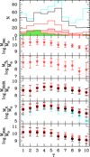Fig. 1.

Number of galaxies and the mean of the log of baryonic, H₂, HI, dust, and stellar masses as a function of morphological stage in our main sample (black lines and filled dots) and in the gaseous sample (red lines and stars symbols). The H I gas mass shown is inside r₂₅. We have not corrected gas masses for helium except for the baryonic masses which include the atomic gas beyond r₂₅. The shaded red and green areas in the upper panel point out the distribution of the number of interacting (92) and active (44 AGN or starbursts) galaxies, respectively, in the gaseous sample. We also show the number of objects and the dust mass distribution for all DustPedia galaxies (cyan lines and filled squares).

– The gaseous sample is representative of the main sample.

– Dust and atomic gas masses peak for Sbc–Sc-type (T = 4–5) galaxies and decline for earlier and later types, while the stellar mass drops more steadily with T. This confirms the results of Rémy-Ruyer et al. (2014, see their appendix) and Nersesian et al. (2019).

– Molecular gas masses follow the distribution of stellar mass, decreasing for high T and underlining the role of stars in enhancing the formation of molecules by compressing the ISM (Blitz & Rosolowsky 2004; Wong et al. 2013).

– The baryonic mass is dominated by stars for earlier-type galaxies, while both gas and stars contribute for later types. The mean value of the baryonic mass decreases by a factor of about ten going from the peak value of 3 × 10¹⁰ M_⊙ for Sb galaxies to the irregular galaxies.

We reiterate that galaxies in the main sample are required to be detected at 250 μm. Thus, our main (and gaseous) sample might be biased against objects with smaller dust masses. Thanks to SED fitting and to the wide wavelength coverage, dust masses are available for most of the DustPedia sample, even for objects not detected or observed at 250 μm (they are missing for only 5% of DustPedia late-type galaxies because of flux-quality requirements; Sect. 3). Even though our main sample includes only 75% of all DustPedia late-type galaxies, the distribution of dust mass versus morphology is compatible with that for the full sample (cyan datapoints in Fig. 1), for all but the later types (which suffer from the flux limit to a greater extent: only 45% of DustPedia galaxies with T ≥ 8 survive the cut). However, we do not expect this bias to significantly affect our results due to the large scatter in the data and to equivalent flux-dependent biases which will not greatly affect the dust-to-star and dust-to-gas ratios (e.g., the 250 μm flux selection leads to a similar overestimation of the stellar mass of later-type galaxies; not shown).

4. The ISM scaling relations in the Local Universe

In this section, we present and discuss different scaling relations between the masses of all ISM components (dust and gas) in combination with the gas-phase metallicities and stellar masses. Even though it is not possible to separate the dust masses associated with each gas phase, here we study the correlation of the total dust mass with atomic and molecular gas separately in order to highlight trends in the ranges where either of the gas components dominates. As explained in the previous sections, all data are uniformly homogenized and all masses refer to the values within r₂₅.

4.1. Scaling relations between the masses of gas and dust

We study the ISM scaling relations between the dust mass and atomic, molecular, and total gas mass under two assumptions on the X_CO conversion factor, that is, by adopting a constant X_CO and a metallicity-dependent one (see Sect. 3.1). In the following plots (Figs. 2 and 3), we fit the data in the logarithmic space:

$\begin{matrix} \log {(M_{gas})}_{r 25} = q + m \times \log {(M_{d})}_{r 25}, \end{matrix}$ $\begin{aligned} \mathrm{log}({M}_{\rm gas})_{r25} = q + m \times \mathrm{log}({M}_{\rm d})_{r25}, \end{aligned}$ (4)

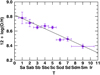Fig. 2.

Scaling relation between dust and HI masses within r₂₅, in logarithmic scale, for 429 DustPedia late-type galaxies (those with dust and HI mass data). The light blue circles are log(M_HI) detections with error bars drawn in light gray. Red squares with downward arrows show log(M_HI) upper limits. The (black) continuum line is the line fit derived for the plotted 429 galaxies, and the (magenta) dashed line that for the sample galaxies with dust, HI, and H₂ data (252 galaxies, those plotted in both panels of Fig. 3). Equations of the line fits and the Pearson correlation coefficients R are also given in the figure.

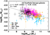Fig. 3.

Left panel: same as Fig. 2 for the scaling relation between dust and H₂ masses for 252 DustPedia late-type galaxies (those with dust and H₂ data). The H₂ gas masses were derived assuming the constant X_CO (value from Bolatto et al. 2013). Right panel: same as left panel but for the scaling relation between dust and total gas masses.

where m and q are the slope and the intercept coefficients of the fit, respectively, and M_gas is the mass of atomic, molecular, or total gas in units of M_⊙. The coefficients of the fits, the Pearson correlation coefficients R, and the number of sample galaxies taken into account for each correlation are given in the figures and in Table 3. Based on the t-test used to establish if the coefficient R is significantly different from zero, we stress that the significance P of all coefficients R provided in this work are P < 0.0001 (i.e., very highly significantly different from zero). All fits in this section are obtained using the “survival analysis” (Feigelson & Babu 2012), which consists in an ensemble of statistical methods that take into account the presence of “censored” data points (in our case, upper limits for ∼18% and ∼2% of the total ¹²CO and H I masses, respectively). We perform the survival analysis using the EM algorithm, available through the Astronomy Survival Analysis (ASURV) package (Feigelson & Nelson 1985; Isobe et al. 1986) in the IRAF⁶ environment (see Yesuf & Ho 2019, for a recent use of the survival analysis in the context of galaxy scaling relations).

Table 3.

Main properties of the fitting lines of the scaling relations presented in Sect. 4.1.

Figure 2 shows that dust and HI masses are well correlated within the optical disk (R = 0.79 − 0.80). The slope of this relationship is sublinear (m = 0.85 ± 0.03, for 429 galaxies) and it remains unchanged if we consider the smaller sample of galaxies with both HI and H₂ data (m = 0.85 ± 0.04, for 252 galaxies). This latter result excludes the presence of possible biases due to a larger sample of galaxies with available HI data with respect to the CO one (see Table 2). The nonlinear relation between dust and HI masses is driven by a few galaxies with low dust-to-HI mass ratio for M_HI < 3 × 10⁹ M_⊙. The left panel of Fig. 3 shows that dust and H₂ masses, under the assumption of the constant X_CO, are well correlated with a linear slope (m = 1.02 ± 0.07, R = 0.72, for 252 galaxies). The significance of the difference between the coefficients R of the dust-HI and dust-H₂ correlations is P-value = 0.0168. Since this P-value is less than 0.05 (significance level of 0.05), we conclude that the two R differ significantly. This allows us to infer that dust and HI are better correlated than dust and H₂. The Right panel of Fig. 3 shows the relationship between dust and total gas masses: a slope of m = 0.91 ± 0.04 (R = 0.84, for 252 galaxies). The significance of the difference between the coefficients R of the dust-HI and dust-total gas correlations is P-value = 0.0949 − 0.1236 (higher than 0.05), meaning that the dust is correlated with HI and total gas with similar statistical significance. On the contrary, the significance of the difference between the coefficients R of the dust-H₂ and dust-total gas correlations is P-value = 0.0005, implying that dust and total gas are better correlated than dust and H₂. We performed a similar analysis with a metallicity-dependent X_CO, finding similar relationships although with lower R, and again a slightly better correlation between dust and total gas masses. The results of the fits and correlation coefficients are collected in Table 3.

An unexpected result emerges from Figs. 2 and 3: within the optical disk of late-type galaxies of the Local Universe, there is a tighter correlation between dust mass and atomic gas mass than between dust mass and molecular gas mass. This is opposite to what is observed at smaller scales in the ISM, where dust and molecular gas are strongly associated in the star formation process, while the H I gas is not directly involved with it. In particular, there is observational evidence of a dependence of the dust–gas relation on the ISM gas phase (molecular or atomic), both in the Milky Way – studied in absorption – and in external galaxies (e.g., Jenkins 2009; Roman-Duval et al. 2014; Chiang & Ménard 2019). For instance, Roman-Duval et al. (2014) found a higher DGR in the dense ISM dominated by molecular gas in the Magellanic Clouds observed at 10−50 pc resolution. Moreover, the distributions of dust, molecular gas, and total gas are rather similar and both generally distributed in a disk, often with an exponential decline of surface density along the radius (e.g., Alton et al. 1998; Bianchi et al. 2000; Bigiel et al. 2008; Muñoz-Mateos et al. 2009; Hunt et al. 2015b; Casasola et al. 2017; Mosenkov et al. 2019). Instead, the HI gas does not generally follow an exponential distribution (see Sect. 3.2). The HI gas often has a decline towards galaxy center (see, e.g., Figs. 3 and A.2 in Casasola et al. 2017), likely due to the rapid transformation of the atomic gas into molecular gas, and then into stars in the denser central parts of galaxies (e.g., Bigiel et al. 2008). The most common trend in galaxies is therefore characterized by HI and molecular gas distributed in a complementary way.

However, the weaker correlation between dust and molecular gas mass might just be the result of the uncertainties in applying a single-recipe aperture correction, and of the scatter around the assumed X_CO conversion factor. For instance, Corbelli et al. (2012) analyzed a sample of 35 metal-rich spirals of the Virgo Cluster and found a stronger correlation between the dust and molecular gas mass than what we find here. The reason might be that half of their objects have direct molecular gas masses from maps, and half estimated from aperture corrections, while in the current work the fraction of the latter is much higher (∼98%). Nevertheless, our results are consistent with those of Corbelli et al. (2012) and agree with the fact that the mass of dust correlates better with the total gas mass than with the single components. An analogous result was found by Orellana et al. (2017) on a sample of 189 galaxies at z < 0.06 with available HI and CO observations.

Another important point is that the assumption of a metallicity-dependent X_CO does not lead to stronger correlations between dust mass and molecular and total gas masses with respect to adopting a constant X_CO. This might be due to the fact that: (i) X_CO does not depend only on metallicity (at least in our metallicity range, with 8 < 12 + log(O/H) < 9.5 dex), and (ii) in our sample of galaxies, spanning a range of morphologies, X_CO might vary along the disk due to different conditions in both metallicity, gas density, and ionizing flux, and thus our assumption of single correction is an over-simplification.

It is worth stressing that if we normalize the dust and gaseous masses using the stellar mass, there is a well-defined scaling relation between the normalized dust mass and the normalized atomic gas while there is no correlation between the normalized dust mass and the normalized molecular mass. The scaling relation between dust and atomic gas masses, both normalized with respect to the stellar mass, is shown in Fig. 4.

Fig. 4.

Same as Fig. 2 but with dust and HI masses normalized with respect to the stellar mass.

Potentially we could compare the scaling relations between dust and gas masses with others present in the literature (see references above). However this comparison makes sense only if done coherently. We decide to not graphically compare our ISM scaling relations with others for the following reasons: (i) dust masses we use are the only ones obtained with the full THEMIS model that can provide dust masses up to two to three times lower than those derived from other commonly used dust models (Draine et al. 2007); (ii) scaling relations involving the gas-phase metallicity are strongly dependent on the adopted calibration (e.g., N2, R₂₃, De Vis et al. 2019); (iii) we use all mass data reported to their values within r₂₅; and (iv) upper limits were treated differently, especially in gas data (e.g., survival analysis, conversion of upper limits in detections under some assumptions). This choice is applied to all scaling relations shown in the paper.

4.2. Scaling relations between stellar and gas mass

In this section, we provide a relationship between gas and stellar mass for our galaxy sample. The main limitation of previous studies has been a lack of molecular gas data. For this reason, most published studies provided gas–star relationships limited to the atomic gas component (e.g., Cortese et al. 2011; Catinella et al. 2013; Gavazzi et al. 2013; De Vis et al. 2017a, an exception to this is the study by Cortese et al. 2016).

In Fig. 5, we show H₂-to-HI gas mass versus HI-to-stellar mass ratios within r₂₅ under the assumption of the constant X_CO. We find an anti-correlation between H₂-to-HI and H I-to-stellar mass ratios: when H₂ dominates over HI (at higher H₂-to-HI values), the galaxies have already formed a large number of stars, and thus their HI-to-stellar mass ratio is low. On the other hand, galaxies dominated by HI are less evolved, and therefore they have a lower stellar mass (a higher HI-to-stellar mass ratio). The relationship within r₂₅ is given by the equation:

$\begin{matrix} log {(M_{HI} / M_{star})}_{r 25} = & (- 1.18 \pm 0.03) \\ + (- 0.57 \pm 0.04) \times log {(M_{H 2} / M_{HI})}_{r 25}, \end{matrix}$ $\begin{aligned} {\log (M_{\rm HI}/M_{\rm star})_{r25}} =&(-1.18 \pm 0.03)\nonumber \\& + {(-0.57 \pm 0.04) \times \log (M_{\rm H2}/M_{\rm HI})_{r25}}, \end{aligned}$ (5)

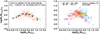Fig. 5.

The HI-to-stellar mass ratio as a function of HI-to-H₂ mass ratio within r₂₅, in logarithmic scale, assuming a constant X_CO (Bolatto et al. 2013). In this plot, we exclude data with HI upper limits (7/252). The black line is the fit to the drawn data.

assuming the constant X_CO (R = 0.70 for 245 sample galaxies). We also derived the scaling relation of Eq. (5) under the assumption of a metallicity-dependent X_CO, finding similar slope and intercept to those by assuming the constant X_CO but with lower Pearson coefficient (R = 0.47).

De Vis et al. (2019) provided a scaling relation similar to that expressed in Eq. (5) using the total HI mass. These correlations allow us to derive the H₂ gas mass (or the total gas mass) for a given galaxy using the H I gas and the stellar masses.

5. Mass ratios in the Local Universe

In this section, we study the mass ratios between the ISM components and their trends as a function of galaxy morphology. Tables 1, 4, and 7 show that all morphologies from T = 1 to T = 10 are well statistically represented in various properties of the ISM. In our analysis we also include stellar mass. In particular, we study the gas fraction (f_gas) defined as the ratio M_tot gas/(M_star + M_tot gas), the molecular-to-atomic gas mass ratio, the dust-to-gas mass ratios separating the various gas phases (atomic, molecular, total gas), and the dust-to-stellar mass ratio. We also explore how the dust-to-total gas mass ratio varies as a function of the molecular-to-atomic gas mass ratio. In the following, we present and discuss these mass ratios on a case-by-case basis. The mean values and the uncertainties of studied ratios have been derived using the survival analysis technique based on the Kaplan-Meier estimator (Kaplan & Meier 1958). These quantities are collected in Tables 4 and 7.

Table 4.

Mean values of the gas fraction, f_gas = M_tot gas/(M_star + M_tot gas), and the molecular-to-atomic gas mass ratio, within r₂₅, expressed in logarithm as a function of the morphological stage from T = 1 to T = 10, and assuming a constant X_CO (Bolatto et al. 2013) and a metallicity-dependent X_CO (Amorín et al. 2016).

5.1. Gas fraction

Figure 6 shows the trend of f_gas within r₂₅ as a function of the morphological stage, assuming a constant and a metallicity-dependent X_CO. The gas fraction with the metallicity-dependent X_CO is higher than that (but always consistent within the errors) with the constant X_CO. The gas fraction increases with increasing T from T = 1 to T = 6, while it remains approximately constant from T = 6 to T = 10. This trend holds for both assumptions on X_CO (see Table 4 for mean values of f_gas).

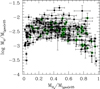Fig. 6.

Gas fraction, f_gas = M_tot gas/(M_star + M_tot gas), within r₂₅ as a function of the morphological stage, from T = 1 to T = 10, assuming a constant X_CO (Bolatto et al. 2013, filled green dots) and a metallicity-dependent X_CO (Amorín et al. 2016, empty red squares). The symbols represent the mean values and their uncertainties (expressed in logarithm) in bins of ΔT = 1, except for the morphological stages T = 8, 9, 10 that are binned together because of a smaller number of later-type galaxies than earlier-type ones.

It is well known that the gas fraction is a proxy for galaxy evolution as it is a good measurement of how much star formation can be sustained from the current gas reservoir, compared to the star formation that has already happened (e.g., De Vis et al. 2017a, 2019). Inflows and outflows of gas and mergers can also affect the gas fraction (e.g., Casasola et al. 2004; Mancillas et al. 2019), and due to them, there is not necessarily a monotonic relation between the gas fraction and the evolutionary stage of a galaxy. The trend shown in Fig. 6 is a direct consequence of the level of evolution of galaxies of different morphological type: early galaxies (Sa-Sb) are usually more evolved than late ones (Sc-Sd-Irr) and thus they have converted a larger fraction of their baryonic mass into stars. On the other hand, late-type galaxies are less evolved than early-type ones since they are characterized by lower star formation efficiencies (see, e.g., Ferrini & Galli 1988; Galli & Ferrini 1989; Matteucci 1994; Mollá & Díaz 2005; Tissera et al. 2005; Brooks et al. 2007; De Rossi et al. 2007; Mouhcine et al. 2008; Tassis et al. 2008; Magrini et al. 2012). The approximately constant trend of f_gas as a function of galaxy morphology for T > 6 galaxies might be due to the fact that our analysis refers to the optical disk, while later-type galaxies (e.g., the irregulars) are typically HI-dominated and this gas is mainly located in the outer parts, beyond r₂₅ (e.g. IC 10, Ashley et al. 2014).

Our results on f_gas as a function of galaxy morphology are consistent with those recently obtained by Sorai et al. (2019) with the COMING⁷ survey, a project based on a sample of 344 FIR bright galaxies of all morphological types from ellipticals to irregulars. Unlike us, Sorai et al. (2019) studied the ratio of the total molecular gas mass to the total baryonic mass, ignoring the atomic gas mass. Although these latter authors found no clear trend of this fraction with the Hubble stage, it tends to decrease in early-type galaxies and vice versa in late-type galaxies.

5.2. Molecular-to-atomic gas mass ratio

Figure 7 shows the variation of M_H2/M_HI as a function of morphological stage within r₂₅, assuming a constant and a metallicity-dependent X_CO. Under both assumptions on X_CO, M_H2/M_HI tends to decrease with increasing T. The blue continuum line and the magenta dashed line are the linear fits for a constant and a metallicity-dependent X_CO assumption, respectively, and they only help to follow the decreasing trends. We do not provide the equation of these fits since the x-axis displays T that is not a numerical physical quantity and it depends on the adopted morphological classification of galaxies. The observed decreasing trend is again consistent with the expected galaxy evolution throughout the various morphological types: early-type galaxies have already transformed their HI in H₂, while late-type but less evolved galaxies remain dominated by atomic gas. We refer to Table 4 for mean values of M_H2/M_HI as a function of T.

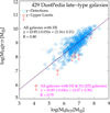Fig. 7.

Molecular-to-atomic gas mass ratio within r₂₅ as a function of the morphological stage, from T = 1 to T = 10, assuming a constant (Bolatto et al. 2013, filled blue circles) and a metallicity-dependent (Amorín et al. 2016, empty magenta squares) X_CO. As in Fig. 6, the symbols represent the mean values and their uncertainties in bins of ΔT = 1, except for the types T = 8, 9, 10 that are binned together. The (blue) continuum line is the linear fit of the data points assuming a constant X_CO, the (magenta) dashed line assuming a metallicity-dependent X_CO.

The decreasing trend of M_H₂/M_HI with increasing morphological stage is consistent with previous literature studies, such as that by Casasola et al. (2004), both for interacting and isolated galaxies (see also Young & Knezek 1989; Young & Scoville 1991; Bettoni et al. 2003). The mean values of M_H₂/M_HI per T are in agreement with those of Casasola et al. (2004) within 2σ. The total mean value of M_H₂/M_HI of our whole sample (log(M_H₂/M_HI) = 0.24) is instead higher than that found by Orellana et al. (2017) for their sample (log(M_H₂/M_HI) = −0.10). This difference might be appointed to the different composition of the two samples: the dataset of Orellana et al. (2017) contains a heterogeneous sample of galaxies, including different morphological types (ellipticals and spirals), isolated and interacting galaxies, and luminosities from normal to ultra-luminous infrared galaxies, while our database is composed of only late-type galaxies. In addition, Orellana et al. (2017) did not provide mean values of M_H₂/M_HI as a function of T for comparison.

5.3. Dust-to-gas mass ratios

Figure 8 shows the trend of the DGR as a function of the morphological stage separating various types of gas (molecular, atomic, total gas), assuming a constant (left panel) and a metallicity-dependent (right panel) X_CO. The drawn black lines are the linear fits to the data and, as in Fig. 7, they only help to follow trends and the corresponding equations of fits are not provided. Figure 8 shows that the dust-to-atomic gas mass ratio decreases with increasing T, and the same trend is followed by the dust-to-total gas mass ratio under both assumptions on X_CO. The dust-to-molecular gas mass ratio instead follows two different trends based on the assumption on X_CO: it increases with increasing T, from T = 1 to T = 10, when adopting a constant X_CO (left panel), while it increases from T = 1 to T = 4 but starts to decrease for T > 4 when assuming a metallicity-dependent X_CO (right panel). The assumption of a metallicity-dependent X_CO better reproduces the expected decrease of the dust-to-total gas mass ratio (e.g., Draine et al. 2007; Rémy-Ruyer et al. 2014; Hunt et al. 2015a; Relaño et al. 2018; De Vis et al. 2019), as the metal content decreases with T (as is also discussed below). However, the trend of dust-to-H₂ mass ratio versus T shown in the Right panel of Fig. 8 is mainly driven by the less populated bin, namely that of the late-type galaxies from Sdm to Ir. We refer to Table 7 for mean values of DGR as a function of T.

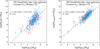Fig. 8.

Left panel: dust-to-gas mass ratio within r₂₅ as a function of the morphological stage, from T = 1 to T = 10, assuming a constant X_CO (Bolatto et al. 2013). All gas types (atomic, molecular, total gas) are considered and separately plotted. Data of individual galaxies are shown in transparency: blue circles are dust/H₂, red squares dust/HI, green triangles dust/total gas. The large symbols represent the mean values (and their uncertainties) in bins of ΔT = 1, except for the types T = 8, 9, 10 that are binned together. The black lines are the linear fits of the trends. Right panel: same as left panel assuming a metallicity-dependent X_CO (Amorín et al. 2016).

Since the gas-phase metallicity is considered to be among the main physical properties of the galaxy driving the DGR (e.g., Rémy-Ruyer et al. 2014), we tested the dependence of the DGR on the gas-phase metallicity, separating the various gas phases and under both assumptions on X_CO, as done for the morphological types. The results of this analysis are illustrated in Fig. 9. The continuum and dashed lines drawn in the two panels of this figure are the fits of the dust-to-total gas mass ratio versus metallicity taking into account all galaxies and excluding the high-metallicity bin, respectively. The trend of DGR as a function of metallicity is similar to that as a function of galaxy morphology (Fig. 8). In addition, the dust-to-H₂ mass ratio is the quantity most affected by the choice of X_CO: while it tends to increase and decrease for low and high metallicity galaxies, respectively, with a constant X_CO, the assumption of a metallicity-dependent X_CO realigns it with the behavior of dust-to-HI and dust-to-total gas mass ratios. The coefficients of these fits are collected in Table 5.

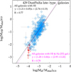Fig. 9.

Left panel: dust-to-gas mass ratio within r₂₅ as a function of the gas-phase metallicity assuming a constant X_CO (Bolatto et al. 2013). Symbols are as in Fig. 8. The large symbols are mean values in metallicity bins, with the bin sizes chosen to include comparable numbers of galaxies. The solid line is the linear fit to all the mean values of the dust-to-total gas mass ratio (big green triangles), while the dashed line is the linear fit to those excluding the high-metallicity bin. Right panel: same as left panel assuming a metallicity-dependent X_CO (Amorín et al. 2016).

Table 5.

Main properties of the fitting lines to DGR within r₂₅ as a function of 12 + log(O/H) shown in Fig. 9, assuming a constant and a metallicity-dependent X_CO and taking into account the total available metallicity range and the restricted one (neglecting the high-metallicity bin).

From Table 5 it emerges that the assumption of the constant X_CO produces a dust-to-total gas mass ratio depending on gas-phase metallicity as DGR ∝ (O/H)^0.3 (continuum line in the left panel of Fig. 9), not in line with theoretical expectations based on a constant dust-to-metal ratio (see e.g., Clark et al. 2019) and predicting a slope of about 1 (see later). The slope becomes 0.7 excluding the high-metallicity bin in the fit (dashed line in the left panel of Fig. 9). On the contrary, assuming a metallicity-dependent X_CO according to the calibration of Amorín et al. (2016), we find DGR ∝ (O/H)^0.7 (continuum line in the right panel of Fig. 9). The DGR becomes ∝(O/H)^1.0 neglecting the high-metallicity bin in the fit (dashed line in the right panel of Fig. 9), which is consistent with several theoretical expectations, mainly those neglecting dust grain growth. We notice that other theoretical studies including dust grain growth predict a slope steeper than 1 (e.g., Zhukovska 2014; Feldmann 2015; Aoyama et al. 2017; De Vis et al. 2017b; McKinnon et al. 2018). We also mention that the slope between DGR and oxygen abundance might be slightly steeper than 1 if the full DustPedia sample is used (see De Vis et al. 2019, and De Vis, priv. comm.).

Several studies have indeed shown that the DGR (also studied with the opposite ratio, the gas-to-dust mass ratio (GDR)) is well represented by a power law with a slope of about 1 (and higher, or ≲ − 1 in terms of GDR) at high metallicities and down to 12 + log(O/H) ∼ 8.0–8.2 (e.g., James et al. 2002; Draine et al. 2007; Galliano et al. 2008; Leroy et al. 2011; Amorín et al. 2016; Giannetti et al. 2017). Rémy-Ruyer et al. (2014) found a GDR versus metallicity relation parametrized as a broken power-law, with a slope of −1 at high-metallicity and a slope of −3.1 ± 1.8 at low-metallicity, with a transition metallicity around 8 (see also Popping et al. 2017, for a model accounting for the double-power-law trend between DGR and gas-phase metallicity of local galaxies). Additionally, spatially resolved studies (e.g., Relaño et al. 2018; Vílchez et al. 2019) have found that the relation between the DGR and 12 + log(O/H) at local scales agrees with the general relation found for nearby galaxies by Rémy-Ruyer et al. (2014). To explain the steeper trend at low metallicities, Rémy-Ruyer et al. (2014) invoked the action of the harder interstellar radiation field in low-metallicity dwarf galaxies that affects the balance between dust formation and destruction by limiting the accretion or enhancing the destruction of the dust grains. However, we stress that our sample is not characterized by very low metallicities (12 + log(O/H) = 7.0−8.0).

Our sample extends up to 12 + log(O/H) = 9.5 (although only for 5.3% of the sample) and the inclusion of these high-metallicity galaxies has the effect of softening the slope of the DGR versus metallicity relation over the entire metallicity range of our sample, providing a slope of 0.7 instead of 1 under the assumption of a metallicity-dependent X_CO. We also stress that the adopted calibration of X_CO with the metallicity from Amorín et al. (2016) is based on galaxy sample with 12 + log(O/H) ≤ 9.0. However, different X_CO prescriptions disagree on what happens in the high-metallicity “uncharted territory”. We also point out that the high-metallicity bin shown in Fig. 9 is the largest one because of the smaller number of galaxies in the extreme of our sample, adding an uncertainty to our results.

To complete the characterization of our galaxy sample in terms of gas-phase metallicity, we also studied the variation of 12 + log(O/H) as a function of the morphological stage. This analysis is complementary to that performed in Figs. 8 and 9 and allows us to better outline the connection between DGR, gas-phase metallicity, and galaxy morphology. The correlation between 12 + log(O/H) and T is shown in Fig. 10 for ∼78% of our sample (339 galaxies). As expected, the oxygen abundance tends to decrease with increasing T (e.g., Cervantes-Sodi & Hernández 2009). In Table 6 we have collected the mean values of 12 + log(O/H) as a function of T for all sample galaxies with metallicity measurements (second column of the table) and for those with data for dust, H₂, and HI (third column of the table, i.e., for the 208 galaxies plotted in the right panel of Fig. 8 and in both panels of Fig. 9). We stress that values of 12 + log(O/H) reported in the second and third columns are consistent, indicating that the mean metallicities for the subsample of galaxies with complete gas and dust information are representative of the mean oxygen abundances, free of bias, for the whole sample.

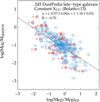Fig. 10.

Oxygen abundance as a function of morphology stage, from T = 1 to T = 10. As in Fig. 6, the symbols represent the mean values (and their uncertainties) in bins of ΔT = 1, except for types T = 8, 9, 10 that are binned together. The black line is the linear fit to the mean values.

Table 6.

Mean values of the metallicity abundances derived from the N2 method (Pettini & Pagel 2004), 12 + log(O/H)_N2, as a function of morphological stage, from T = 1 to T = 10.

Combining Figs. 8–10 it emerges that DGR, galaxy morphology, and oxygen abundance are closely related properties. By assuming the metallicity-dependent X_CO, the DGR decreases with increasing morphological stage and with decreasing oxygen abundance. These two decrements are quite similar and are able to reproduce the expected trends of DGR versus T, and DGR versus 12 + log(O/H). We also show that the effect of a variable X_CO mainly affects the extremes of our sample, in particular the most metal-rich bin populated by Sa-Sb galaxies, thus altering the global slopes of the relationships of DGR versus metallicity and DGR versus morphological type. The most populated regions of our sample, dominated by late-type galaxies with solar metallicity, are less affected by the choice of X_CO. Based on these findings, we suggest using a metallicity-dependent X_CO, especially for studies dedicated to the DGR of nearby late-type galaxies.

5.4. Dust-to-stellar mass ratio

In Fig. 11, we present the relationship between M_dust/M_star and M_star, dividing sample galaxies as a function of four main morphological stages. There is a clear anti-correlation between M_dust/M_star and M_star, which is already known in the literature (Cortese et al. 2012; Clemens et al. 2013; Clark et al. 2015; Calura et al. 2017; De Vis et al. 2017a; Orellana et al. 2017) and has been reproduced by both chemical evolutionary models (see, e.g., Cortese et al. 2012; Calura et al. 2017; De Vis et al. 2017a) and cosmological hydro simulations (Camps et al. 2016). The fit to our sample is given in the following equation:

$\begin{matrix} log (M_{dust} / M_{star}) = & (- 0.36 \pm 0.23) \\ + (- 0.27 \pm 0.02) \times log (M_{star} [M_{⊙}]) . \end{matrix}$ $\begin{aligned} {\log (M_{\rm dust}/M_{\rm star})} =&(-0.36 \pm 0.23)\nonumber \\& + {(-0.27 \pm 0.02) \times \log (M_{\rm star}[M_\odot ])}. \end{aligned}$ (6)

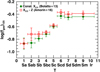Fig. 11.

Dust-to-stellar mass ratio as a function of stellar mass. Galaxies are drawn with different symbols as a function of morphological stage (four bins in galaxy morphology). The continuum line is the linear fit to the DustPedia late-type galaxy sample (Eq. (6)).

The anti-correlation displayed in Fig. 11 and quantified in Eq. (6) suggests that galaxies with a lower stellar mass have higher dust-to-stellar mass ratios with respect to stellar mass than their more massive counterparts. This can be interpreted in terms of the dust lifecycle: both stars and dust are products of star formation but while stellar mass grows with time as the galaxy evolves, dust grains (and the metals from which they form, along with the other ISM components) eventually disappear from the budget as they are incorporated into the stellar mass. This also agrees with the trend of the DGR versus gas-phase metallicity displayed in Fig. 9. Interestingly, Calura et al. (2017) found that the anti-correlation between M_dust/M_star and M_star is not only valid for the Local Universe but continues to exist up to redshfit z ∼ 2.

Figure 11 also shows the trend in terms of morphological distribution. As already noticed by Cortese et al. (2012), the dust-to-stellar mass ratio monotonically decreases when moving from late- to early-type galaxies. da Cunha et al. (2010) explain how this trend is in line with the decreasing specific SFR (sSFR, SFR per unit of M_star) with increasing M_star (e.g., Schiminovich et al. 2007; Catinella et al. 2018). Although the study of the sSFR is beyond the scope of this work, it is worth reiterating that low-stellar-mass late-type galaxies have typically high sSFR and gas fraction. The gas is able to fuel the star formation, and subsequently large amounts of dust are formed. For high-stellar-mass earlier-type galaxies, the sSFR and gas fraction instead tend to decrease, and consequently the production of dust is lower and likely not able to compensate for or exceed that destroyed in the ISM during these processes. Figure 11 also shows that Sa-Sab galaxies are almost all below the line fit but tend to cover the entire range of M_star. This could explain the diagonal scatter around the fit line. Sb-Sdm galaxies instead appear to lie more coherently around the fit line, and Sm-Irr galaxies, although they tend to follow the general trend, contribute to the diagonal scatter around the fit line with galaxies below it, especially those with lower M_star.

Figure 12 shows the trend of log(M_dust/M_star) as a function of morphological stage. The dust-to-stellar mass ratio increases with increasing T, from T = 1 to T = 6, and remains approximately constant within the uncertainties (or slightly decreases) from T = 6 to T = 10. This trend is similar to that found for f_gas as a function of T (see Fig. 6), suggesting – together with scaling relations – that the dust mass, total gas mass, stellar mass, and morphology of galaxies might be directly linked. This aspect has already been pointed out by Cortese et al. (2012), although restricted to the atomic gas instead of the total gas. However, unlike us, Cortese et al. (2012) found that M_dust/M_star continues rising up to Sm (T = 9) galaxies, although this increase is softer than that of earlier-type galaxies. This disagreement could be due to the different adopted dust models and/or different treatment of data. Table 7 presents the mean values of the dust-to-stellar mass ratio as a function of morphological stage.

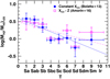Fig. 12.

Dust-to-stellar mass ratio as a function of the morphological stage, from T = 1 to T = 10. As in Fig. 6 the symbols represent the mean values (and their uncertainties) in bins of ΔT = 1, except for types T = 8, 9, 10 that are binned together.

Table 7.

Mean values of the dust-to-gas mass ratio (separating molecular, atomic, and total gas) and dust-to-stellar gas mass ratio within r₂₅, in logarithmic scale, as a function of the morphological stage, from T = 1 to T = 10.

5.5. Dust-to-total gas mass ratio versus molecular-to-atomic gas mass ratio

We also explored a new – to our knowledge – combination of mass ratios. Having a well-defined gaseous sample with both HI and H₂ data over more than two orders of magnitude, we can study the dust-to-total gas mass ratio as a function of the molecular-to-atomic gas mass ratio within r₂₅, or equivalently, as a function of the fraction of gas in molecular form f_mol (= M_H2/(M_H2 + M_HI), or (1.36 × M_H2)/M_tot gas if the total gas mass includes the helium contribution, as in the present work). We want to stress that though the relation DGR versus H₂/HI mass ratio might not have been published so far, the dependence of the DGR on the ISM gas phase (or gas density) has previously been explored as already mentioned in Sect. 4.1 (e.g., Jenkins 2009; Roman-Duval et al. 2014; Chiang & Ménard 2019). The results of this analysis are shown in Figs. 13 and 14 and refer to the gaseous sample. From these figures it emerges that data are distributed along a hill-like shape.

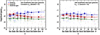Fig. 13.

Left panel: dust-to-total gas mass ratio as a function of the molecular-to-atomic gas mass ratio within r₂₅ for the gas sample. The small, transparent green circles and red squares are data points assuming a constant and a metallicity-dependent X_CO, respectively. These data points are drawn without error bars. The large symbols are the means of y-axis values in bins of x-axis values. Right panel: same as left panel, under the assumption of the constant X_CO and displaying data points as a function of morphological stage (four main bins in galaxy morphology).

First, we note that the shape of the distribution is mostly independent of how we model the X_CO conversion factor (Left panel of Fig. 13). Therefore, the downward side for high M_H2/M_HI is not biased by the larger uncertainties on X_CO for the high-metallicity earlier-type galaxies that populate this part of the plot (see Fig. 10 and later in this section). The upward-sloping side of the hill-like distribution cannot be traced properly using a metallicity-dependent X_CO because of the lack of metal-abundance determinations in galaxies with a low M_H2/M_HI. Therefore, in the following discussion, for the sake of simplicity, we discuss the results obtained with a constant X_CO.

Assuming a constant X_CO for the whole galaxy sample, we would expect a flat slope of the DGR versus M_H2/M_HI, within the errors. On the other hand, we expect both M_H2/M_HI and DRG to increase in more evolved galaxies since atomic gas is transformed into molecular gas and then into stars. The presence of stars increases the hydrostatic pressures in the disk, favoring the formation of denser molecular clouds (e.g., Elmegreen 1993; Krumholz et al. 2009; Wong et al. 2013). In addition, during the latest phases of their evolution, stars pollute the ISM with metals and dust. Thus, while the increasing trend on the left-side of the plot is in line with the above-mentioned expectations, the right-most part of the plot is instead more puzzling, showing a decrease of DGR for the more evolved/molecular-gas-dominated galaxies.

Since the gas masses are used in the quantities plotted on both axes, we checked the influence of the errors (and in particular those on molecular gas mass) in the trends we detected. With a Monte Carlo procedure, we derived mock values for the gas and dust masses: for atomic and molecular gas, the random values are obtained from the true values and their uncertainty; for dust, we assumed a constant DGR (we used the average value at the peak of the hill-like distribution curve) and derived random values from the true total gas mass and the average uncertainty on M_dust. The average trend for this “null hypothesis”, obtained after 1000 representations of the dataset, provides an approximatively constant DGR as a function of M_H2/M_HI. Indeed the large errors can produce a downward trend for high M_H2/M_HI, but never to the level we detected in the true dataset, and therefore the observed trend is real.

In the right panel of Fig. 13, we investigate how the different morphological types are distributed over the hill-like curve. While galaxies with intermediate morphological type from Sb to Sd are located all across the curve, Sm and Ir galaxies are predominantly located towards to left-side of the plot where H I is the dominant gas phase and the dust is still in small quantities with respect to the total gas, and the early-type Sa and Sab are located on the right-side where the H₂ component dominates. The galaxy evolution highlighted by the right panel of Fig. 13 is consistent with that of Fig. 11, and confirms that galaxies with higher H₂/HI mass ratios are bulge-dominated systems as found, for instance, with COLD GASS and xGASS surveys (e.g, Saintonge et al. 2016; Catinella et al. 2018).

The unexpected decrease of DGR in H₂-dominated galaxies can be due to the interplay of different effects:

(i) Dust might be destroyed by strong stellar radiation fields or by shocks at a rate that is higher than the consumption of the ISM components during the astration process; in fact, many of these H₂-dominated galaxies also contain a lot of hot X-ray emitting gas and dust grains could be destroyed by collisional sputtering by the hot gas atoms (e.g., Jones 2004).

(ii) The emission cross-section of dust grains associated to the molecular component could be smaller than that in HI-rich environments. Indeed, a pilot study on two resolved DustPedia galaxies finds a reduced cross section in regions of high gas surface density (Clark et al. 2019). If this is confirmed, and if the grain cross-section in molecular clouds is smaller than the THEMIS value calibrated on FIR observations of the Milky Way high-Galactic latitude cirrus, the current values of the dust mass for H₂-rich galaxies, therefore also the D/H ratios, could be underestimated. We discuss this issue further in a companion paper (Bianchi et al. 2019).

(iii) Most of the active galaxies have high molecular fractions, as shown in Fig. 14. In addition, some HI-deficient galaxies undergoing an interaction with the intercluster medium are also located in the right-hand tail of Fig. 14. Active galaxies might have an H₂ enhancement in the center (e.g., Casasola et al. 2008, 2011) and the use of a uniform radial scale-length for the whole gaseous sample might overestimate the molecular mass and the gas molecular fraction. However, some of the active galaxies are also starburst and might indeed have a real enhancement of the molecular gas fraction while most of the dust is destroyed by the intense radiation field mentioned in (i). For H I-deficient galaxies dust and HI might be removed from the optical disk during the interaction with the intercluster medium (e.g., Cortese et al. 2010; Corbelli et al. 2012) while they often retain their molecular content or even enhance it by gas compression. Therefore, we expect them to have a lower dust-to-gas mass ratio if the galaxy is intrinsically H₂ dominated. As shown by Stark et al. (2013), galaxies with a high molecular fraction often have a blue central region often referred to as mass-corrected blue-centeredness which is linked to enhanced star formation and external perturbations.

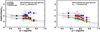Fig. 14.

Dust-to-total gas mass ratio as a function of the molecular fraction within r₂₅ is shown for the gaseous sample. A constant X_CO has been used. The open (green) circles underline active galaxies in the sample.

(iv) The adoption of the Galactic X_CO conversion factor, both constant and metallicity-dependent, for the whole sample could also partially contribute to explain the decrease of DGR in some H₂-dominated galaxies. As mentioned in (iii), some of these galaxies are also starburst where the molecular gas is typically warmer, denser, and with higher column densities than in the Milky Way and in less active objects (e.g., Bradford et al. 2003; Ward et al. 2003; Rangwala et al. 2011). These physical conditions of the gas produce a lower X_CO conversion factor (X_CO ∼ 0.4 × 10²⁰ cm⁻² (K km s⁻¹)⁻¹, e.g., Downes & Solomon 1998; Papadopoulos et al. 2012; Bolatto et al. 2013) than the Galactic one, and therefore a higher DGR for some galaxies located in the decreasing part of the hill-like distribution shown in Fig. 13.

It is well known that also the presence of a companion galaxy and/or a stellar bar can affect this trend as well as the other scaling relations presented above (e.g., Braine & Combes 1993; Combes et al. 1994; Casasola et al. 2004; Di Matteo et al. 2007; Khoperskov et al. 2018; Moreno et al. 2019, and many others). However, a detailed analysis on these aspects is beyond the scope of this paper, and will be addressed in future publications within the DustPedia collaboration.

To our knowledge, no simulation or theory papers make predictions for the resulting DGR versus H₂/HI distribution. Our analysis therefore provides new constraints for cosmological models of galaxy evolution.

6. Summary and final remarks

We present a study on the main ISM scaling relations for the nearby late-type galaxies of the Local Universe. We also discuss important mass ratios. The analysis is based on the DustPedia galaxy sample and the DustPedia dataset, including M_d, M_star, oxygen abundance, and galaxy morphology. Molecular and atomic gas data were extracted from the literature and uniformly homogenized. All the masses are reported to their value within r₂₅. The scaling relations and mass ratios involving molecular gas mass were explored under the assumption of both a constant and a metallicity-dependent X_CO. Our analysis provides new constraints for cosmological models of galaxy evolution and a reference for high-redshift studies. Our main results can be summarized as follows.

Dust and total gas are better correlated than dust and molecular gas, or dust and atomic gas. Dust and atomic gas are better correlated than dust and molecular gas, and this is opposite to what is observed at smaller scales in the ISM. All these scaling relations have a higher Pearson correlation coefficient under the assumption of a constant X_CO than under the assumption of a metallicity-dependent one.
Combining HI, H₂, and stellar masses, we provide general gas-star scaling relations for late-type galaxies of the Local Universe. These gas-star scaling relations allow us to derive the mass of a gas phase (typically the H₂) given the mass of the other gas phase and the stellar mass for a given galaxy.
We provide a characterization of the following mass ratios as a function of morphological stage: gas fraction, molecular-to-atomic gas mass ratio, DGR, and dust-to-stellar mass ratio. Among these mass ratios, only DGR shows a different behavior based on the assumption on X_CO.
Only the assumption of the metallicity-dependent X_CO is able to reproduce the expected decrease in the DGR as a function of galaxy morphology and gas-phase metallicity. Our analysis shows that DGR, gas-phase metallicity, and galaxy morphology are properties that are directly linked. Based on these findings, we recommend the use of a metallicity-dependent X_CO, especially to characterize DGR.
We explore a novel trend between DGR and molecular-to-atomic gas mass ratio. The data are distributed along a hill-like curve for both assumptions on X_CO, where the gas molecular fraction and the DGR show a positive correlation for low molecular gas fractions, while this trend breaks down for molecular-rich galaxies. We suggest several different scenarios to interpret this finding.

¹

D₂₅ is the major axis isophote at which the optical surface brightness falls beneath 25 mag arcsec⁻² (we also use here r₂₅ = D₂₅/2).

²

The DustPedia database is available at http://dustpedia.astro.noa.gr/

³

R1 is the radius where the H I surface density (Σ_HI) is equal to 1 M_⊙ pc⁻².

⁴

Version 0.12.1, available at https://cigale.lam.fr

⁵

The Heterogeneous Evolution Model for Interstellar Solids, http://www.ias.u-psud.fr/themis/index.html

⁶

IRAF (Image Reduction and Analysis Facility) is distributed by the National Optical Astronomy Observatory, which is operated by the Association of Universities for Research in Astronomy (AURA) under a cooperative agreement with the National Science Foundation.

⁷

COMING is CO Multi-line Imaging of Nearby Galaxies, a Nobeyama Radio Observatory legacy project performed with the 45 m telescope.

Acknowledgments

We are grateful to the anonymous referee, whose comments and suggestions improved the quality of this manuscript. The authors would like to thank A. Giannetti and F. Calura for helpful discussions. DustPedia is a collaborative focused research project supported by the European Union under the Seventh Framework Programme (2007-2013) call (proposal no. 606824). The participating institutions are: Cardiff University, UK; National Observatory of Athens, Greece; Ghent University, Belgium; Université Paris Sud, France; National Institute for Astrophysics, Italy and CEA (Paris), France. We acknowledge funding from the INAF PRIN-SKA 2017 program 1.05.01.88.04. We acknowledge funding from the INAF main stream 2018 program “Gas-DustPedia: A definitive view of the ISM in the Local Universe”. VC, SB, and EC acknowledge the support from grant PRIN MIUR 2017 – 20173ML3WW_s. This research made use of the NASA/IPAC Extragalactic Database (NED), which is operated by the Jet Propulsion Laboratory, California Institute of Technology, under contract with the National Aeronautics and Space Administration. This research has made use of the VizieR catalogue access tool, CDS, Strasbourg, France. The original description of the VizieR service was published in Ochsenbein et al. (2000). We acknowledge the usage of the HyperLeda database (http://leda.univ-lyon1.fr).

References

Aalto, S., Booth, R. S., Black, J. H., Koribalksi, B., & Wielebinksi, R. 1994, A&A, 286, 365 [NASA ADS] [Google Scholar]
Accurso, G., Saintonge, A., Catinella, B., et al. 2017, MNRAS, 470, 4750 [NASA ADS] [Google Scholar]
Albrecht, M., Chini, R., Krügel, E., Müller, S. A. H., & Lemke, R. 2004, A&A, 414, 141 [NASA ADS] [CrossRef] [EDP Sciences] [Google Scholar]
Alton, P. B., Trewhella, M., Davies, J. I., et al. 1998, A&A, 335, 807 [NASA ADS] [Google Scholar]
Amorín, R., Muñoz-Tuñón, C., Aguerri, J. A. L., & Planesas, P. 2016, A&A, 588, A23 [NASA ADS] [CrossRef] [EDP Sciences] [Google Scholar]
Aoyama, S., Hou, K.-C., Shimizu, I., et al. 2017, MNRAS, 466, 105 [NASA ADS] [CrossRef] [Google Scholar]
Arimoto, N., Sofue, Y., & Tsujimoto, T. 1996, PASJ, 48, 275 [NASA ADS] [CrossRef] [Google Scholar]
Ashley, T., Elmegreen, B. G., Johnson, M., et al. 2014, AJ, 148, 130 [NASA ADS] [CrossRef] [Google Scholar]
Asplund, M., Grevesse, N., Sauval, A. J., & Scott, P. 2009, ARA&A, 47, 481 [NASA ADS] [CrossRef] [Google Scholar]
Bahé, Y. M., Crain, R. A., Kauffmann, G., et al. 2016, MNRAS, 456, 1115 [NASA ADS] [CrossRef] [Google Scholar]
Bajaja, E., WielebinKSi, R., Reuter, H.-P., Harnett, J. I., & Hummel, E. 1995, A&AS, 114, 147 [NASA ADS] [Google Scholar]
Barone, L. T., Heithausen, A., Hüttemeister, S., Fritz, T., & Klein, U. 2000, MNRAS, 317, 649 [NASA ADS] [CrossRef] [Google Scholar]
Bettoni, D., Galletta, G., García-Burillo, S., & Rodríguez-Franco, A. 2001, A&A, 374, 421 [NASA ADS] [CrossRef] [EDP Sciences] [Google Scholar]
Bettoni, D., Galletta, G., & García-Burillo, S. 2003, A&A, 405, 5 [NASA ADS] [CrossRef] [EDP Sciences] [Google Scholar]
Bianchi, S., Davies, J. I., Alton, P. B., Gerin, M., & Casoli, F. 2000, A&A, 353, L13 [NASA ADS] [Google Scholar]
Bianchi, S., De Vis, P., Viaene, S., et al. 2018, A&A, 620, A112 [NASA ADS] [CrossRef] [EDP Sciences] [Google Scholar]
Bianchi, S., Casasola, V., Baes, M., et al. 2019, A&A, 631, A102 [NASA ADS] [CrossRef] [EDP Sciences] [Google Scholar]
Bigiel, F., & Blitz, L. 2012, ApJ, 756, 183 [NASA ADS] [CrossRef] [Google Scholar]
Bigiel, F., Leroy, A., Walter, F., et al. 2008, AJ, 136, 2846 [NASA ADS] [CrossRef] [Google Scholar]
Blitz, L., & Rosolowsky, E. 2004, ApJ, 612, L29 [NASA ADS] [CrossRef] [Google Scholar]
Bolatto, A. D., Leroy, A. K., RosolowKSy, E., Walter, F., & Blitz, L. 2008, ApJ, 686, 948 [NASA ADS] [CrossRef] [Google Scholar]
Bolatto, A. D., Wolfire, M., & Leroy, A. K. 2013, ARA&A, 51, 207 [Google Scholar]
Boquien, M., Burgarella, D., Roehlly, Y., et al. 2019, A&A, 622, A103 [NASA ADS] [CrossRef] [EDP Sciences] [Google Scholar]
Boselli, A., Lequeux, J., & Gavazzi, G. 2002, Ap&SS, 281, 127 [NASA ADS] [CrossRef] [Google Scholar]
Boselli, A., Cortese, L., & Boquien, M. 2014, A&A, 564, A65 [NASA ADS] [CrossRef] [EDP Sciences] [Google Scholar]
Bourne, N., Dunne, L., Bendo, G. J., et al. 2013, MNRAS, 436, 479 [NASA ADS] [CrossRef] [Google Scholar]
Bradford, C. M., Nikola, T., Stacey, G. J., et al. 2003, ApJ, 586, 891 [NASA ADS] [CrossRef] [Google Scholar]
Braine, J., & Combes, F. 1993, A&A, 269, 7 [NASA ADS] [Google Scholar]
Brinchmann, J., Charlot, S., White, S. D. M., et al. 2004, MNRAS, 351, 1151 [NASA ADS] [CrossRef] [Google Scholar]
Brooks, A. M., Governato, F., Booth, C. M., et al. 2007, ApJ, 655, L17 [NASA ADS] [CrossRef] [Google Scholar]
Calette, A. R., Avila-Reese, V., Rodríguez-Puebla, A., Hernández-Toledo, H., & Papastergis, E. 2018, Rev. Mex. Astron. Astrofis., 54, 443 [NASA ADS] [Google Scholar]
Calura, F., Pozzi, F., Cresci, G., et al. 2017, MNRAS, 465, 54 [NASA ADS] [CrossRef] [Google Scholar]
Camps, P., Trayford, J. W., Baes, M., et al. 2016, MNRAS, 462, 1057 [CrossRef] [Google Scholar]
Casasola, V., Bettoni, D., & Galletta, G. 2004, A&A, 422, 941 [NASA ADS] [CrossRef] [EDP Sciences] [Google Scholar]
Casasola, V., Combes, F., Bettoni, D., & Galletta, G. 2007, A&A, 473, 771 [NASA ADS] [CrossRef] [EDP Sciences] [Google Scholar]
Casasola, V., Combes, F., García-Burillo, S., et al. 2008, A&A, 490, 61 [NASA ADS] [CrossRef] [EDP Sciences] [Google Scholar]
Casasola, V., Hunt, L. K., Combes, F., et al. 2010, A&A, 510, A52 [NASA ADS] [CrossRef] [EDP Sciences] [Google Scholar]
Casasola, V., Hunt, L. K., Combes, F., García-Burillo, S., & Neri, R. 2011, A&A, 527, A92 [NASA ADS] [CrossRef] [EDP Sciences] [Google Scholar]
Casasola, V., Hunt, L., Combes, F., & García-Burillo, S. 2015, A&A, 577, A135 [NASA ADS] [CrossRef] [EDP Sciences] [Google Scholar]
Casasola, V., Cassarà, L. P., Bianchi, S., et al. 2017, A&A, 605, A18 [NASA ADS] [CrossRef] [EDP Sciences] [Google Scholar]
Catinella, B., Schiminovich, D., Kauffmann, G., et al. 2012, A&A, 544, A65 [NASA ADS] [CrossRef] [EDP Sciences] [Google Scholar]
Catinella, B., Schiminovich, D., Cortese, L., et al. 2013, MNRAS, 436, 34 [NASA ADS] [CrossRef] [Google Scholar]
Catinella, B., Saintonge, A., Janowiecki, S., et al. 2018, MNRAS, 476, 875 [NASA ADS] [CrossRef] [Google Scholar]
Cayatte, V., Kotanyi, C., BalkowKSi, C., & van Gorkom, J. H. 1994, AJ, 107, 1003 [NASA ADS] [CrossRef] [Google Scholar]
Cervantes-Sodi, B., & Hernández, X. 2009, Rev. Mex. Astron. Astrofis., 45, 75 [NASA ADS] [Google Scholar]
Chiang, Y.-K., & Ménard, B. 2019, ApJ, 870, 120 [NASA ADS] [CrossRef] [Google Scholar]
Chu, T. S., Wilson, R. W., England, R. W., Gray, D. A., & Legg, W. E. 1978, Bell Sys. Tech. J., 57, 1257 [CrossRef] [Google Scholar]
Clark, C. J. R., Dunne, L., Gomez, H. L., et al. 2015, MNRAS, 452, 397 [NASA ADS] [CrossRef] [Google Scholar]
Clark, C. J. R., Verstocken, S., Bianchi, S., et al. 2018, A&A, 609, A37 [NASA ADS] [CrossRef] [EDP Sciences] [Google Scholar]
Clark, C. J. R., De Vis, P., Baes, M., et al. 2019, MNRAS, 489, 5256 [NASA ADS] [CrossRef] [Google Scholar]
Claussen, M. J., & Sahai, R. 1992, AJ, 103, 1134 [NASA ADS] [CrossRef] [Google Scholar]
Clemens, M. S., Negrello, M., De Zotti, G., et al. 2013, MNRAS, 433, 695 [NASA ADS] [CrossRef] [Google Scholar]
Cook, M., Evoli, C., Barausse, E., Granato, G. L., & Lapi, A. 2010, MNRAS, 402, 941 [NASA ADS] [CrossRef] [Google Scholar]
Cook, R. H. W., Cortese, L., Catinella, B., et al. 2019, MNRAS, 2391 [Google Scholar]
Combes, F., Prugniel, P., Rampazzo, R., & Sulentic, J. W. 1994, A&A, 281, 725 [NASA ADS] [Google Scholar]
Combes, F., Young, L. M., & Bureau, M. 2007, MNRAS, 377, 1795 [NASA ADS] [CrossRef] [Google Scholar]
Combes, F., Baker, A. J., Schinnerer, E., et al. 2009, A&A, 503, 73 [NASA ADS] [CrossRef] [EDP Sciences] [Google Scholar]
Corbelli, E., Bianchi, S., Cortese, L., et al. 2012, A&A, 542, A32 [NASA ADS] [CrossRef] [EDP Sciences] [Google Scholar]
Cormier, D., Madden, S. C., Lebouteiller, V., et al. 2014, A&A, 564, A121 [NASA ADS] [CrossRef] [EDP Sciences] [Google Scholar]
Cortese, L., Davies, J. I., Pohlen, M., et al. 2010, A&A, 518, L49 [NASA ADS] [CrossRef] [EDP Sciences] [Google Scholar]
Cortese, L., Catinella, B., Boissier, S., Boselli, A., & Heinis, S. 2011, MNRAS, 415, 1797 [NASA ADS] [CrossRef] [Google Scholar]
Cortese, L., Ciesla, L., Boselli, A., et al. 2012, A&A, 540, A52 [NASA ADS] [CrossRef] [EDP Sciences] [Google Scholar]
Cortese, L., Bekki, K., Boselli, A., et al. 2016, MNRAS, 459, 3574 [NASA ADS] [CrossRef] [Google Scholar]
Crain, R. A., Bahé, Y. M., Lagos, C. D. P., et al. 2017, MNRAS, 464, 4204 [NASA ADS] [CrossRef] [Google Scholar]
da Cunha, E., Eminian, C., Charlot, S., & Blaizot, J. 2010, MNRAS, 403, 1894 [NASA ADS] [CrossRef] [Google Scholar]
Daddi, E., Dickinson, M., Morrison, G., et al. 2007, ApJ, 670, 156 [NASA ADS] [CrossRef] [Google Scholar]
Dahlem, M., Golla, G., Whiteoak, J. B., et al. 1993, A&A, 270, 29 [NASA ADS] [Google Scholar]
Davé, R., Oppenheimer, B. D., & Finlator, K. 2011, MNRAS, 415, 11 [NASA ADS] [CrossRef] [Google Scholar]
Davies, J. I., Baes, M., Bianchi, S., et al. 2017, PASP, 129, 044102 [NASA ADS] [CrossRef] [EDP Sciences] [Google Scholar]
De Rossi, M. E., Tissera, P. B., De Lucia, G., & Kauffmann, G. 2007, Boletin de la Asociacion Argentina de Astronomia La Plata Argentina, 50, 235 [NASA ADS] [Google Scholar]
Devereux, N. A., & Young, J. S. 1990, ApJ, 350, L25 [NASA ADS] [CrossRef] [Google Scholar]
De Vis, P., Dunne, L., Maddox, S., et al. 2017a, MNRAS, 464, 4680 [NASA ADS] [CrossRef] [Google Scholar]
De Vis, P., Gomez, H. L., Schofield, S. P., et al. 2017b, MNRAS, 471, 1743 [NASA ADS] [CrossRef] [Google Scholar]
De Vis, P., Jones, A., Viaene, S., et al. 2019, A&A, 623, A5 [NASA ADS] [CrossRef] [EDP Sciences] [Google Scholar]
Diemer, B., Stevens, A. R. H., Lagos, C. D. P., et al. 2019, MNRAS, 487, 1529 [NASA ADS] [CrossRef] [Google Scholar]
Di Matteo, P., Combes, F., Melchior, A.-L., et al. 2007, A&A, 468, 61 [NASA ADS] [CrossRef] [EDP Sciences] [Google Scholar]
Djorgovski, S., & Davis, M. 1987, ApJ, 313, 59 [NASA ADS] [CrossRef] [Google Scholar]
Downes, D., & Solomon, P. M. 1998, ApJ, 507, 615 [NASA ADS] [CrossRef] [Google Scholar]
Draine, B. T., Dale, D. A., Bendo, G., et al. 2007, ApJ, 663, 866 [NASA ADS] [CrossRef] [Google Scholar]
Dunne, L., & Eales, S. A. 2001, MNRAS, 327, 697 [NASA ADS] [CrossRef] [Google Scholar]
Dutton, A. A. 2009, MNRAS, 396, 121 [NASA ADS] [CrossRef] [Google Scholar]
Dutton, A. A., & van den Bosch, F. C. 2009, MNRAS, 396, 141 [NASA ADS] [CrossRef] [Google Scholar]
Dutton, A. A., van den Bosch, F. C., Dekel, A., & Courteau, S. 2007, ApJ, 654, 27 [NASA ADS] [CrossRef] [Google Scholar]
Elbaz, D., Daddi, E., Le Borgne, D., et al. 2007, A&A, 468, 33 [NASA ADS] [CrossRef] [EDP Sciences] [Google Scholar]
Elfhag, T., Booth, R. S., Hoeglund, B., Johansson, L. E. B., & Sandqvist, A. 1996, A&AS, 115, 439 [NASA ADS] [Google Scholar]
Elmegreen, B. G. 1993, ApJ, 411, 170 [NASA ADS] [CrossRef] [Google Scholar]
Erb, D. K. 2008, ApJ, 674, 151 [NASA ADS] [CrossRef] [Google Scholar]
Erb, D. K., Shapley, A. E., Pettini, M., et al. 2006, ApJ, 644, 813 [NASA ADS] [CrossRef] [Google Scholar]
Espada, D., Verley, S., Miura, R. E., et al. 2019, ApJ, 887, 88 [NASA ADS] [CrossRef] [Google Scholar]
Feigelson, E. D., & Babu, G. J. 2012, in Modern Statistical Methods for Astronomy (Cambridge, UK: Cambridge University Press) [Google Scholar]
Feigelson, E. D., & Nelson, P. I. 1985, ApJ, 293, 192 [NASA ADS] [CrossRef] [Google Scholar]
Feldmann, R. 2015, MNRAS, 449, 3274 [NASA ADS] [CrossRef] [Google Scholar]
Ferrini, F., & Galli, D. 1988, A&A, 195, 27 [NASA ADS] [Google Scholar]
Fu, J., Hou, J. L., Yin, J., & Chang, R. X. 2009, ApJ, 696, 668 [NASA ADS] [CrossRef] [Google Scholar]
Fu, J., Guo, Q., Kauffmann, G., & Krumholz, M. R. 2010, MNRAS, 409, 515 [NASA ADS] [CrossRef] [Google Scholar]
Galli, D., & Ferrini, F. 1989, A&A, 218, 31 [NASA ADS] [Google Scholar]
Galliano, F., Dwek, E., & Chanial, P. 2008, ApJ, 672, 214 [NASA ADS] [CrossRef] [Google Scholar]
Galliano, F., Galametz, M., & Jones, A. P. 2018, ARA&A, 56, 673 [NASA ADS] [CrossRef] [Google Scholar]
Garnett, D. R., & Shields, G. A. 1987, ApJ, 317, 82 [NASA ADS] [CrossRef] [Google Scholar]
Gavazzi, G., Fumagalli, M., Fossati, M., et al. 2013, A&A, 553, A89 [NASA ADS] [CrossRef] [EDP Sciences] [Google Scholar]
Genzel, R., Tacconi, L. J., Combes, F., et al. 2012, ApJ, 746, 69 [NASA ADS] [CrossRef] [Google Scholar]
Giannetti, A., Leurini, S., König, C., et al. 2017, A&A, 606, L12 [NASA ADS] [CrossRef] [EDP Sciences] [Google Scholar]
Ginolfi, M., Hunt, L. K., Tortora, C., Schneider, R., & Cresci, G. 2019, A&A, submitted [arXiv:1907.06654] [Google Scholar]
Glover, S. C. O., & Mac Low, M.-M. 2011, MNRAS, 412, 337 [NASA ADS] [CrossRef] [MathSciNet] [Google Scholar]
Gnedin, N. Y., Tassis, K., & Kravtsov, A. V. 2009, ApJ, 697, 55 [NASA ADS] [CrossRef] [Google Scholar]
Gomez de Castro, A. I., & Garcia-Burillo, S. 1997, A&A, 322, 381 [NASA ADS] [Google Scholar]
Gong, M., Ostriker, E. C., & Kim, C.-G. 2018, ApJ, 858, 16 [NASA ADS] [CrossRef] [Google Scholar]
Haynes, M. P., & Giovanelli, R. 1984, AJ, 89, 758 [NASA ADS] [CrossRef] [Google Scholar]
Henry, A., Scarlata, C., Domínguez, A., et al. 2013, ApJ, 776, L27 [NASA ADS] [CrossRef] [Google Scholar]
Horellou, C., Casoli, F., & Dupraz, C. 1995, A&A, 303, 361 [NASA ADS] [Google Scholar]
Hunt, L. K., Testi, L., Casasola, V., et al. 2014, A&A, 561, A49 [NASA ADS] [CrossRef] [EDP Sciences] [Google Scholar]
Hunt, L. K., García-Burillo, S., Casasola, V., et al. 2015a, A&A, 583, A114 [NASA ADS] [CrossRef] [EDP Sciences] [Google Scholar]
Hunt, L. K., Draine, B. T., Bianchi, S., et al. 2015b, A&A, 576, A33 [NASA ADS] [CrossRef] [EDP Sciences] [Google Scholar]
Hunt, L. K., Weiß, A., Henkel, C., et al. 2017, A&A, 606, A99 [Google Scholar]
Isobe, T., Feigelson, E. D., & Nelson, P. I. 1986, ApJ, 306, 490 [NASA ADS] [CrossRef] [Google Scholar]
Israel, F. P. 1992, A&A, 265, 487 [NASA ADS] [Google Scholar]
Israel, F. 2000, Molecular Hydrogen in Space (Cambridge: Cambridge University Press), 293 [Google Scholar]
Israel, F. P., Tacconi, L. J., & Baas, F. 1995, A&A, 295, 599 [NASA ADS] [Google Scholar]
James, A., Dunne, L., Eales, S., & Edmunds, M. G. 2002, MNRAS, 335, 753 [NASA ADS] [CrossRef] [Google Scholar]
Jenkins, E. B. 2009, ApJ, 700, 1299 [NASA ADS] [CrossRef] [Google Scholar]
Jones, A. P. 2004, Astrophys. Dust, 309, 347 [NASA ADS] [Google Scholar]
Jones, A. P., Köhler, M., Ysard, N., et al. 2017, A&A, 602, A46 [NASA ADS] [CrossRef] [EDP Sciences] [Google Scholar]
Jorgensen, I., Franx, M., & Kjaergaard, P. 1996, MNRAS, 280, 167 [NASA ADS] [CrossRef] [Google Scholar]
Kaplan, E. L., & Meier, P. 1958, J. Am. Stat. Assoc., 53, 457 [Google Scholar]
Kauffmann, G. 1996, MNRAS, 281, 475 [NASA ADS] [CrossRef] [Google Scholar]
Kauffmann, G., Li, C., Fu, J., et al. 2012, MNRAS, 422, 997 [NASA ADS] [CrossRef] [Google Scholar]
Kenney, J. D., & Young, J. S. 1988, ApJS, 66, 261 [NASA ADS] [CrossRef] [Google Scholar]
Kenney, J. D. P., & Young, J. S. 1989, ApJ, 344, 171 [NASA ADS] [CrossRef] [Google Scholar]
Kenney, J. D. P., Young, J. S., Hasegawa, T., & Nakai, N. 1990, ApJ, 353, 460 [NASA ADS] [CrossRef] [Google Scholar]
Kennicutt, Jr., R. C. 1998a, ARA&A, 36, 189 [Google Scholar]
Kennicutt, Jr., R. C. 1998b, ApJ, 498, 541 [NASA ADS] [CrossRef] [Google Scholar]
Khoperskov, S., Haywood, M., Di Matteo, P., et al. 2018, A&A, 609, A60 [NASA ADS] [CrossRef] [EDP Sciences] [Google Scholar]
Kobulnicky, H. A., Kennicutt, Jr., R. C., & Pizagno, J. L. 1999, ApJ, 514, 544 [NASA ADS] [CrossRef] [Google Scholar]
Kohno, K., Ishizuki, S., Matsushita, S., Vila-Vilaró, B., & Kawabe, R. 2003, PASJ, 55, L1 [NASA ADS] [CrossRef] [Google Scholar]
Krumholz, M. R., McKee, C. F., & Tumlinson, J. 2009, ApJ, 693, 216 [NASA ADS] [CrossRef] [Google Scholar]
Kuno, N., Sato, N., Nakanishi, H., et al. 2007, PASJ, 59, 117 [NASA ADS] [Google Scholar]
Kutner, M. L., & Ulich, B. L. 1981, ApJ, 250, 341 [NASA ADS] [CrossRef] [Google Scholar]
Lagos, C. D. P., Lacey, C. G., Baugh, C. M., Bower, R. G., & Benson, A. J. 2011a, MNRAS, 416, 1566 [NASA ADS] [CrossRef] [Google Scholar]
Lagos, C. D. P., Baugh, C. M., Lacey, C. G., et al. 2011b, MNRAS, 418, 1649 [NASA ADS] [CrossRef] [Google Scholar]
Lequeux, J., Peimbert, M., Rayo, J. F., Serrano, A., & Torres-Peimbert, S. 1979, A&A, 80, 155 [Google Scholar]
Leroy, A. K., Walter, F., Brinks, E., et al. 2008, AJ, 136, 2782 [NASA ADS] [CrossRef] [Google Scholar]
Leroy, A. K., Walter, F., Bigiel, F., et al. 2009, AJ, 137, 4670 [NASA ADS] [CrossRef] [Google Scholar]
Leroy, A. K., Bolatto, A., Gordon, K., et al. 2011, ApJ, 737, 12 [NASA ADS] [CrossRef] [Google Scholar]
Lin, L., Pan, H.-A., Ellison, S. L., et al. 2019, ApJ, 884, L33 [NASA ADS] [CrossRef] [Google Scholar]
Lisenfeld, U., Espada, D., Verdes-Montenegro, L., et al. 2011, A&A, 534, A102 [NASA ADS] [CrossRef] [EDP Sciences] [Google Scholar]
Lisenfeld, U., Xu, C. K., Gao, Y., et al. 2019, A&A, 627, A107 [NASA ADS] [CrossRef] [EDP Sciences] [Google Scholar]
Madden, S. C., Rémy-Ruyer, A., Galametz, M., et al. 2013, PASP, 125, 600 [NASA ADS] [CrossRef] [Google Scholar]
Magrini, L., Bianchi, S., Corbelli, E., et al. 2011, A&A, 535, A13 [NASA ADS] [CrossRef] [EDP Sciences] [Google Scholar]
Magrini, L., Hunt, L., Galli, D., et al. 2012, MNRAS, 427, 1075 [NASA ADS] [CrossRef] [Google Scholar]
Maier, C., Lilly, S. J., Ziegler, B. L., et al. 2014, ApJ, 792, 3 [NASA ADS] [CrossRef] [Google Scholar]
Maier, C., Ziegler, B. L., Lilly, S. J., et al. 2015, A&A, 577, A14 [NASA ADS] [CrossRef] [EDP Sciences] [Google Scholar]
Maier, C., Kuchner, U., Ziegler, B. L., et al. 2016, A&A, 590, A108 [NASA ADS] [CrossRef] [EDP Sciences] [Google Scholar]
Maiolino, R., Ruiz, M., Rieke, G. H., & Papadopoulos, P. 1997, ApJ, 485, 552 [NASA ADS] [CrossRef] [Google Scholar]
Makarov, D., Prugniel, P., Terekhova, N., Courtois, H., & Vauglin, I. 2014, A&A, 570, A13 [CrossRef] [EDP Sciences] [Google Scholar]
Mancillas, B., Combes, F., & Duc, P.-A. 2019, A&A, 630, A112 [NASA ADS] [CrossRef] [EDP Sciences] [Google Scholar]
Marinacci, F., Grand, R. J. J., Pakmor, R., et al. 2017, MNRAS, 466, 3859 [NASA ADS] [CrossRef] [Google Scholar]
Martinsson, T. P. K., Verheijen, M. A. W., Westfall, K. B., et al. 2013, A&A, 557, A131 [NASA ADS] [CrossRef] [EDP Sciences] [Google Scholar]
Matteucci, F. 1994, A&A, 288, 57 [NASA ADS] [Google Scholar]
McKinnon, R., Vogelsberger, M., Torrey, P., Marinacci, F., & Kannan, R. 2018, MNRAS, 478, 2851 [NASA ADS] [CrossRef] [Google Scholar]
Mollá, M., & Díaz, A. I. 2005, MNRAS, 358, 521 [NASA ADS] [CrossRef] [Google Scholar]
Moreno, J., Torrey, P., Ellison, S. L., et al. 2019, MNRAS, 485, 1320 [NASA ADS] [CrossRef] [Google Scholar]
Mosenkov, A. V., Baes, M., Bianchi, S., et al. 2019, A&A, 622, A132 [NASA ADS] [CrossRef] [EDP Sciences] [Google Scholar]
Mouhcine, M., Gibson, B. K., Renda, A., & Kawata, D. 2008, A&A, 486, 711 [NASA ADS] [CrossRef] [EDP Sciences] [Google Scholar]
Moustakas, J., & Kennicutt, Jr., R. C. 2006, ApJS, 164, 81 [NASA ADS] [CrossRef] [Google Scholar]
Moustakas, J., Kennicutt, Jr., R. C., Tremonti, C. A., et al. 2010, ApJS, 190, 233 [NASA ADS] [CrossRef] [Google Scholar]
Muñoz-Mateos, J. C., Gil de Paz, A., Boissier, S., et al. 2009, ApJ, 701, 1965 [NASA ADS] [CrossRef] [Google Scholar]
Narayanan, D., Krumholz, M. R., Ostriker, E. C., & Hernquist, L. 2012, MNRAS, 421, 3127 [NASA ADS] [CrossRef] [Google Scholar]
Nersesian, A., Xilouris, E. M., Bianchi, S., et al. 2019, A&A, 624, A80 [NASA ADS] [CrossRef] [EDP Sciences] [Google Scholar]
Noeske, K. G., Weiner, B. J., Faber, S. M., et al. 2007, ApJ, 660, L43 [Google Scholar]
Noll, S., Burgarella, D., Giovannoli, E., et al. 2009, A&A, 507, 1793 [NASA ADS] [CrossRef] [EDP Sciences] [Google Scholar]
Ochsenbein, F., Bauer, P., & Marcout, J. 2000, A&AS, 143, 23 [NASA ADS] [CrossRef] [EDP Sciences] [Google Scholar]
Orellana, G., Nagar, N. M., Elbaz, D., et al. 2017, A&A, 602, A68 [NASA ADS] [CrossRef] [EDP Sciences] [Google Scholar]
O’Sullivan, E., Combes, F., Salomé, P., et al. 2018, A&A, 618, A126 [NASA ADS] [CrossRef] [EDP Sciences] [Google Scholar]
Papadopoulos, P. P., van der Werf, P., Xilouris, E., et al. 2012, ApJ, 751, 10 [NASA ADS] [CrossRef] [Google Scholar]
Peng, Y.-J., Lilly, S. J., Kovač, K., et al. 2010, ApJ, 721, 193 [NASA ADS] [CrossRef] [Google Scholar]
Pettini, M., & Pagel, B. E. J. 2004, MNRAS, 348, L59 [NASA ADS] [CrossRef] [Google Scholar]
Pilyugin, L. S., Contini, T., & Vílchez, J. M. 2004, A&A, 423, 427 [NASA ADS] [CrossRef] [EDP Sciences] [Google Scholar]
Planesas, P., Gomez-Gonzalez, J., & Martin-Pintado, J. 1989, A&A, 216, 1 [NASA ADS] [Google Scholar]
Pohlen, M., Cortese, L., Smith, M. W. L., et al. 2010, A&A, 518, L72 [NASA ADS] [CrossRef] [EDP Sciences] [Google Scholar]
Popping, G., Somerville, R. S., & Galametz, M. 2017, MNRAS, 471, 3152 [NASA ADS] [CrossRef] [Google Scholar]
Power, C., Baugh, C. M., & Lacey, C. G. 2010, MNRAS, 406, 43 [NASA ADS] [CrossRef] [Google Scholar]
Rahman, N., Bolatto, A. D., Xue, R., et al. 2012, ApJ, 745, 183 [NASA ADS] [CrossRef] [Google Scholar]
Rangwala, N., Maloney, P. R., Glenn, J., et al. 2011, ApJ, 743, 94 [NASA ADS] [CrossRef] [Google Scholar]
Relaño, M., De Looze, I., Kennicutt, R. C., et al. 2018, A&A, 613, A43 [NASA ADS] [CrossRef] [EDP Sciences] [Google Scholar]
Remy, Q., Grenier, I. A., Marshall, D. J., & Casandjian, J. M. 2017, A&A, 601, A78 [NASA ADS] [CrossRef] [EDP Sciences] [Google Scholar]
Rémy-Ruyer, A., Madden, S. C., Galliano, F., et al. 2014, A&A, 563, A31 [NASA ADS] [CrossRef] [EDP Sciences] [Google Scholar]
Roberts, M. S., Hogg, D. E., Bregman, J. N., Forman, W. R., & Jones, C. 1991, ApJS, 75, 751 [NASA ADS] [CrossRef] [Google Scholar]
Rodighiero, G., Renzini, A., Daddi, E., et al. 2014, MNRAS, 443, 19 [NASA ADS] [CrossRef] [Google Scholar]
Roehlly, Y., Burgarella, D., Buat, V., et al. 2014, in Astronomical Data Analysis Software and Systems XXIII, eds. N. Manset, & P. Forshay, ASP Conf. Ser., 485, 347 [NASA ADS] [Google Scholar]
Roman-Duval, J., Gordon, K. D., Meixner, M., et al. 2014, ApJ, 797, 86 [NASA ADS] [CrossRef] [Google Scholar]
Sage, L. J. 1993a, A&A, 272, 123 [NASA ADS] [Google Scholar]
Sage, L. J. 1993b, A&AS, 100, 537 [NASA ADS] [Google Scholar]
Sakamoto, K., Ho, P. T. P., & Peck, A. B. 2006, ApJ, 644, 862 [NASA ADS] [CrossRef] [Google Scholar]
Saintonge, A., Kauffmann, G., Kramer, C., et al. 2011a, MNRAS, 415, 32 [NASA ADS] [CrossRef] [Google Scholar]
Saintonge, A., Kauffmann, G., Wang, J., et al. 2011b, MNRAS, 415, 61 [NASA ADS] [CrossRef] [Google Scholar]
Saintonge, A., Catinella, B., Cortese, L., et al. 2016, MNRAS, 462, 1749 [NASA ADS] [CrossRef] [Google Scholar]
Salim, S., Lee, J. C., Davé, R., & Dickinson, M. 2015, ApJ, 808, 25 [NASA ADS] [CrossRef] [Google Scholar]
Sánchez, S. F., Barrera-Ballesteros, J. K., Sánchez-Menguiano, L., et al. 2017, MNRAS, 469, 2121 [NASA ADS] [CrossRef] [Google Scholar]
Sandstrom, K. M., Leroy, A. K., Walter, F., et al. 2013, ApJ, 777, 5 [NASA ADS] [CrossRef] [Google Scholar]
Santini, P., Fontana, A., Grazian, A., et al. 2009, A&A, 504, 751 [NASA ADS] [CrossRef] [EDP Sciences] [Google Scholar]
Santini, P., Maiolino, R., Magnelli, B., et al. 2014, A&A, 562, A30 [NASA ADS] [CrossRef] [EDP Sciences] [Google Scholar]
Santini, P., Fontana, A., Castellano, M., et al. 2017, ApJ, 847, 76 [NASA ADS] [CrossRef] [Google Scholar]
Savage, B. D., & Sembach, K. R. 1996, ApJ, 470, 893 [NASA ADS] [CrossRef] [Google Scholar]
Schiminovich, D., Wyder, T. K., Martin, D. C., et al. 2007, ApJS, 173, 315 [NASA ADS] [CrossRef] [Google Scholar]
Schmidt, M. 1959, ApJ, 129, 243 [NASA ADS] [CrossRef] [Google Scholar]
Schmidt, M. 1963, ApJ, 137, 758 [NASA ADS] [CrossRef] [Google Scholar]
Schreiber, C., Pannella, M., Elbaz, D., et al. 2015, A&A, 575, A74 [NASA ADS] [CrossRef] [EDP Sciences] [Google Scholar]
Schruba, A., Leroy, A. K., Walter, F., et al. 2011, AJ, 142, 37 [NASA ADS] [CrossRef] [Google Scholar]
Schruba, A., Leroy, A. K., Walter, F., et al. 2012, AJ, 143, 138 [NASA ADS] [CrossRef] [Google Scholar]
Scoville, N., Arnouts, S., Aussel, H., et al. 2013, ApJS, 206, 3 [NASA ADS] [CrossRef] [Google Scholar]
Sorai, K., Kuno, N., Muraoka, K., et al. 2019, PASJ, in press [arXiv:1910.03863] [Google Scholar]
Speagle, J. S., Steinhardt, C. L., Capak, P. L., & Silverman, J. D. 2014, ApJS, 214, 15 [NASA ADS] [CrossRef] [Google Scholar]
Stark, A. A., Knapp, G. R., Bally, J., et al. 1986, ApJ, 310, 660 [NASA ADS] [CrossRef] [Google Scholar]
Stark, D. V., Kannappan, S. J., Wei, L. H., et al. 2013, ApJ, 769, 82 [NASA ADS] [CrossRef] [Google Scholar]
Stevens, A. R. H., Diemer, B., Lagos, C. D. P., et al. 2019, MNRAS, 483, 5334 [NASA ADS] [CrossRef] [Google Scholar]
Tasca, L. A. M., Le Fèvre, O., Hathi, N. P., et al. 2015, A&A, 581, A54 [NASA ADS] [CrossRef] [EDP Sciences] [Google Scholar]
Tassis, K., Kravtsov, A. V., & Gnedin, N. Y. 2008, ApJ, 672, 888 [NASA ADS] [CrossRef] [Google Scholar]
Tissera, P. B., De Rossi, M. E., & Scannapieco, C. 2005, MNRAS, 364, L38 [NASA ADS] [CrossRef] [Google Scholar]
Tomczak, A. R., Quadri, R. F., Tran, K.-V. H., et al. 2016, ApJ, 817, 118 [NASA ADS] [CrossRef] [Google Scholar]
Tremonti, C. A., Heckman, T. M., Kauffmann, G., et al. 2004, ApJ, 613, 898 [NASA ADS] [CrossRef] [Google Scholar]
Trčka, A., Baes, M., Camp, P., et al. 2019, MNRAS, submitted [Google Scholar]
Tully, R. B., & Fisher, J. R. 1977, A&A, 54, 661 [NASA ADS] [Google Scholar]
van der Laan, T. P. R., Schinnerer, E., Boone, F., et al. 2011, A&A, 529, A45 [NASA ADS] [CrossRef] [EDP Sciences] [Google Scholar]
Vila-Costas, M. B., & Edmunds, M. G. 1992, MNRAS, 259, 121 [NASA ADS] [CrossRef] [Google Scholar]
Vila-Vilaro, B., Cepa, J., & Zabludoff, A. 2015, ApJS, 218, 28 [NASA ADS] [CrossRef] [Google Scholar]
Vílchez, J. M., Relaño, M., Kennicutt, R., et al. 2019, MNRAS, 483, 4968 [NASA ADS] [CrossRef] [Google Scholar]
Wang, J., Kauffmann, G., Józsa, G. I. G., et al. 2013, MNRAS, 433, 270 [NASA ADS] [CrossRef] [Google Scholar]
Wang, J., Fu, J., Aumer, M., et al. 2014, MNRAS, 441, 2159 [NASA ADS] [CrossRef] [Google Scholar]
Ward, J. S., Zmuidzinas, J., Harris, A. I., et al. 2003, ApJ, 587, 171 [NASA ADS] [CrossRef] [Google Scholar]
Wilson, C. D. 1995, ApJ, 448, L97 [NASA ADS] [CrossRef] [Google Scholar]
Wilson, C. D., Warren, B. E., Israel, F. P., et al. 2012, MNRAS, 424, 3050 [NASA ADS] [CrossRef] [Google Scholar]
Whitaker, K. E., Franx, M., Leja, J., et al. 2014, ApJ, 795, 104 [NASA ADS] [CrossRef] [MathSciNet] [Google Scholar]
Wolfire, M. G., Hollenbach, D., & McKee, C. F. 2010, ApJ, 716, 1191 [NASA ADS] [CrossRef] [Google Scholar]
Wong, T., Xue, R., Bolatto, A. D., et al. 2013, ApJ, 777, L4 [NASA ADS] [CrossRef] [Google Scholar]
Yesuf, H. M., & Ho, L. C. 2019, ApJ, 884, 177 [NASA ADS] [CrossRef] [Google Scholar]
Young, J. S., & Knezek, P. M. 1989, ApJ, 347, L55 [NASA ADS] [CrossRef] [Google Scholar]
Young, J. S., & Scoville, N. Z. 1991, ARA&A, 29, 581 [NASA ADS] [CrossRef] [Google Scholar]
Young, J. S., Xie, S., Tacconi, L., et al. 1995, ApJS, 98, 219 [NASA ADS] [CrossRef] [Google Scholar]
Young, L. M., Bureau, M., Davis, T. A., et al. 2011, MNRAS, 414, 940 [NASA ADS] [CrossRef] [Google Scholar]
Zhukovska, S. 2014, A&A, 562, A76 [NASA ADS] [CrossRef] [EDP Sciences] [Google Scholar]
Zuo, P., Xu, C. K., Yun, M. S., et al. 2018, ApJS, 237, 2 [NASA ADS] [CrossRef] [Google Scholar]

Appendix A: H I and CO observations

In this section, we collect the main properties of our gas data in three tables. Table A.1 lists references consulted for ¹²CO data, Tables A.2 and A.3 list telescopes and main observational properties characterizing ¹²CO and HI data, respectively.

Table A.1.

Sources of ¹²CO data collected for this work.

Table A.2.

Main properties of the telescopes used for the collected ¹²CO data.

Table A.3.

Telescopes and beams used for the collected HI data.

Appendix B: Caveats

In this section, we list possible caveats and systematic uncertainties associated with the analysis and results presented above. These can arise from our simplified assumptions that are not able to completely represent the physics occurring in the ISM and from the adopted methodologies to derive the various physical quantities.

B.1. Caveats concerning the derivation of the ¹²CO emission within the optical disk and of the molecular gas mass

Most of the collected ¹²CO data are observations of one position towards the galaxy center (see Sect. 3.1), from which we derived the corresponding ¹²CO flux within r₂₅ assuming an exponential radial and vertical distribution, central peak, with a scale-length of h_CO/r₂₅ = 0.17 ± 0.03 (Casasola et al. 2017) and a scale-height of z_CO/r₂₅ = 1/100 (Boselli et al. 2014, see Sect. 3.1.1). The adopted value for the molecular gas scale-length, although consistent with those derived in other works, may not be fully representative of a large galaxy sample, spanning a wide range of galaxy properties, such as that presented in this work. As already discussed in Sect. 3.1.1, the exponential decline of ¹²CO is the most common trend in galaxies but all distributions have been observed. The value assumed for the scale-height of ¹²CO is expected to be subject to a larger uncertainty since its determination is based on a small number of galaxies (see Sect. 3.1.1). Despite the uncertainty on h_CO/r₂₅, we preferred to take into account the vertical distribution of the molecular gas. We also checked the location of sample galaxies to which no radial corrections have been applied (e.g., NGC 1068, NGC 4013) in the main plots of our work, such as Figs. 9 and 13. These galaxies cover different regions of the plots confirming that the resulting trends are real and not driven by assumptions on the ¹²CO distribution in the galactic disk. We also stress that Corbelli et al. (2012) studied a sample of 18 galaxies mapped in ¹²CO together with a sample of 17 galaxies where the total ¹²CO flux was determined in a similar way to in our study. Corbelli et al. (2012) did not report differences between the two samples in terms of relationship between dust and molecular or total gas content noticing that galaxies with total derived ¹²CO flux are very well represented by exponential functions (see also Kuno et al. 2007).

We derived M(H₂) by adopting both a constant and a metallicity-dependent X_CO conversion factor. Both assumptions suffer from systematic uncertainties which propagate to the M_H₂ estimate. The choice of a constant X_CO is supported by studies of “normal” galaxies which return similar values in Milky Way-like disks, but with greater scatter and systematic uncertainty. However, departures from the Galactic conversion factor are both observed and expected, and estimates of “typical” values of X_CO in the Milky Way and other spiral galaxies range from ∼1.5 × 10²⁰ cm⁻² (K km s⁻¹)⁻¹ to ∼4 × 10²⁰ cm⁻² (K km s⁻¹)⁻¹ (see references quoted in Sect. 3.1). We decided to adopt a constant X_CO for the sake of uniformity and simplicity, as suggested in the review of Bolatto et al. (2013) in the absence of a detailed characterization of X_CO in a given galaxy and as typically done in the major portion of studies aimed at determining molecular gas mass from ¹²CO line intensities. However, within the DustPedia collaboration we also uniformly derived the oxygen abundances of the entire DustPedia galaxy sample which allowed us to take into account the dependence of X_CO on the metallicity. This clearly adds further uncertainties due to the method used to derive the metallicity (see later Appendix B.3) and the chosen X_CO-metallicity calibration (see Sect. 3.3).

Galaxies with available ¹²CO data coming from ¹²CO(2–1) or ¹²CO(3–2) emission lines could be affected by an uncertainty due to the assumption of a mean ratio between ¹²CO emission lines, and not determined for a given galaxy. Without precise knowledge of ¹²CO line ratios for all galaxies, we indeed adopted typical ratios present in the literature (see Sect. 3.1). However, we signal that only 4.7% of the ¹²CO data come from ¹²CO(2–1) and ¹²CO(3–2) transitions.

Data of ¹²CO coming from interferometric observations (see Table A.2) can also suffer from an additional uncertainty. An interferometer is limited by the minimum spacing of its antennas. Because two antennas cannot be placed closer than some minimum distance (D_min), signals on spatial scales larger than some size (∝λ/D_min) will be attenuated. This effect, called the “missing flux” problem, is typically resolved by using single-dish observations to compute short spacings and complete the interferometric measurements (see e.g., Casasola et al. 2008, 2010, 2011; Combes et al. 2009; van der Laan et al. 2011, as examples of ¹²CO short-spacing corrections). Unfortunately the interferometric ¹²CO observations that we collected in this work are not corrected for short spacings, but they only represent ∼1.2% of ¹²CO data.

B.2. Caveats concerning the derivation of the HI emission within the optical disk

As presented in Sect. 3.2, we derived the HI emission within the optical disk following the method of Wang et al. (2014), who developed an empirical model to describe the observed exponential HI profiles as a function of radius in the outer parts of the galaxy with a depression towards the center. Wang et al. (2014) have also compared their results with existing smoothed particle hydrodynamical simulations and semi-analytic models of disk galaxy formation in a Λ cold dark matter Universe. Both the hydro simulations and the semi-analytic models are able to reproduce the HI surface density profiles and the HI size-mass relation without further tuning of the simulation and model inputs. The “Universal” outer disk profiles in the semi-analytic methods originate from the combination of the assumption that infalling gas has an exponential profile and of the inside-out growth of disks (e.g., Kauffmann 1996; Dutton et al. 2007; Fu et al. 2009). The limit of these findings is that the assumption that gas accreted from the halo is distributed over the disk with an exponential profile has no a priori physical justification. As pointed out by Wang et al. (2014), the fact that the hydrodynamical simulations, at least those presented by Wang et al. (2014), have outer disks that agree so well with the observed “Universal” outer exponential profiles seen in the data is therefore somewhat incomprehensible. The explanation likely lies in the complex interplay between the infall of new gas, star formation, supernova feedback, and gas inflow processes occurring in the simulation.

B.3. Caveats concerning the gas-phase metallicity derivation

As mentioned in Sect. 3.3, we adopted gas-phase metallicity determinations from the empirical calibration N2 of Pettini & Pagel (2004). These metallicities were extracted from De Vis et al. (2019), who compared the results from different empirical and theoretical methods to understand any systematic differences that may result from using various methods. There are limitations linked to the type of metallicity calibration. For example, the empirical calibrations, like the N2 one, are only valid for the same range of excitation and metallicity as the HII regions that were used to build the calibration. Since they are determined assuming an electron temperature, these methods may systematically underestimate the true metallicity if there are temperature inhomogeneities in a galaxy (e.g., De Vis et al. 2019).

All Tables

Table 1.

Classification of the main properties of the DustPedia late-type galaxy sample.

In the text

Table 2.

Total data collected for the studied galaxy sample.

In the text

Table 3.

Main properties of the fitting lines of the scaling relations presented in Sect. 4.1.

In the text

Table 4.

Mean values of the gas fraction, f_gas = M_tot gas/(M_star + M_tot gas), and the molecular-to-atomic gas mass ratio, within r₂₅, expressed in logarithm as a function of the morphological stage from T = 1 to T = 10, and assuming a constant X_CO (Bolatto et al. 2013) and a metallicity-dependent X_CO (Amorín et al. 2016).

In the text

Table 5.

Main properties of the fitting lines to DGR within r₂₅ as a function of 12 + log(O/H) shown in Fig. 9, assuming a constant and a metallicity-dependent X_CO and taking into account the total available metallicity range and the restricted one (neglecting the high-metallicity bin).

In the text

Table 6.

Mean values of the metallicity abundances derived from the N2 method (Pettini & Pagel 2004), 12 + log(O/H)_N2, as a function of morphological stage, from T = 1 to T = 10.

In the text

Table 7.

Mean values of the dust-to-gas mass ratio (separating molecular, atomic, and total gas) and dust-to-stellar gas mass ratio within r₂₅, in logarithmic scale, as a function of the morphological stage, from T = 1 to T = 10.

In the text

Table A.1.

Sources of ¹²CO data collected for this work.

In the text

Table A.2.

Main properties of the telescopes used for the collected ¹²CO data.

In the text

Table A.3.

Telescopes and beams used for the collected HI data.

In the text

All Figures

Fig. 1.

Number of galaxies and the mean of the log of baryonic, H₂, HI, dust, and stellar masses as a function of morphological stage in our main sample (black lines and filled dots) and in the gaseous sample (red lines and stars symbols). The H I gas mass shown is inside r₂₅. We have not corrected gas masses for helium except for the baryonic masses which include the atomic gas beyond r₂₅. The shaded red and green areas in the upper panel point out the distribution of the number of interacting (92) and active (44 AGN or starbursts) galaxies, respectively, in the gaseous sample. We also show the number of objects and the dust mass distribution for all DustPedia galaxies (cyan lines and filled squares).

In the text

Fig. 2.

Scaling relation between dust and HI masses within r₂₅, in logarithmic scale, for 429 DustPedia late-type galaxies (those with dust and HI mass data). The light blue circles are log(M_HI) detections with error bars drawn in light gray. Red squares with downward arrows show log(M_HI) upper limits. The (black) continuum line is the line fit derived for the plotted 429 galaxies, and the (magenta) dashed line that for the sample galaxies with dust, HI, and H₂ data (252 galaxies, those plotted in both panels of Fig. 3). Equations of the line fits and the Pearson correlation coefficients R are also given in the figure.

In the text

	Fig. 3. Left panel: same as Fig. 2 for the scaling relation between dust and H₂ masses for 252 DustPedia late-type galaxies (those with dust and H₂ data). The H₂ gas masses were derived assuming the constant X_CO (value from Bolatto et al. 2013). Right panel: same as left panel but for the scaling relation between dust and total gas masses.
In the text

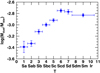	Fig. 4. Same as Fig. 2 but with dust and HI masses normalized with respect to the stellar mass.
In the text

	Fig. 5. The HI-to-stellar mass ratio as a function of HI-to-H₂ mass ratio within r₂₅, in logarithmic scale, assuming a constant X_CO (Bolatto et al. 2013). In this plot, we exclude data with HI upper limits (7/252). The black line is the fit to the drawn data.
In the text

Fig. 6.

Gas fraction, f_gas = M_tot gas/(M_star + M_tot gas), within r₂₅ as a function of the morphological stage, from T = 1 to T = 10, assuming a constant X_CO (Bolatto et al. 2013, filled green dots) and a metallicity-dependent X_CO (Amorín et al. 2016, empty red squares). The symbols represent the mean values and their uncertainties (expressed in logarithm) in bins of ΔT = 1, except for the morphological stages T = 8, 9, 10 that are binned together because of a smaller number of later-type galaxies than earlier-type ones.

In the text

Fig. 7.

Molecular-to-atomic gas mass ratio within r₂₅ as a function of the morphological stage, from T = 1 to T = 10, assuming a constant (Bolatto et al. 2013, filled blue circles) and a metallicity-dependent (Amorín et al. 2016, empty magenta squares) X_CO. As in Fig. 6, the symbols represent the mean values and their uncertainties in bins of ΔT = 1, except for the types T = 8, 9, 10 that are binned together. The (blue) continuum line is the linear fit of the data points assuming a constant X_CO, the (magenta) dashed line assuming a metallicity-dependent X_CO.

In the text

Fig. 8.

Left panel: dust-to-gas mass ratio within r₂₅ as a function of the morphological stage, from T = 1 to T = 10, assuming a constant X_CO (Bolatto et al. 2013). All gas types (atomic, molecular, total gas) are considered and separately plotted. Data of individual galaxies are shown in transparency: blue circles are dust/H₂, red squares dust/HI, green triangles dust/total gas. The large symbols represent the mean values (and their uncertainties) in bins of ΔT = 1, except for the types T = 8, 9, 10 that are binned together. The black lines are the linear fits of the trends. Right panel: same as left panel assuming a metallicity-dependent X_CO (Amorín et al. 2016).

In the text

Fig. 9.

Left panel: dust-to-gas mass ratio within r₂₅ as a function of the gas-phase metallicity assuming a constant X_CO (Bolatto et al. 2013). Symbols are as in Fig. 8. The large symbols are mean values in metallicity bins, with the bin sizes chosen to include comparable numbers of galaxies. The solid line is the linear fit to all the mean values of the dust-to-total gas mass ratio (big green triangles), while the dashed line is the linear fit to those excluding the high-metallicity bin. Right panel: same as left panel assuming a metallicity-dependent X_CO (Amorín et al. 2016).

In the text

	Fig. 10. Oxygen abundance as a function of morphology stage, from T = 1 to T = 10. As in Fig. 6, the symbols represent the mean values (and their uncertainties) in bins of ΔT = 1, except for types T = 8, 9, 10 that are binned together. The black line is the linear fit to the mean values.
In the text

	Fig. 11. Dust-to-stellar mass ratio as a function of stellar mass. Galaxies are drawn with different symbols as a function of morphological stage (four bins in galaxy morphology). The continuum line is the linear fit to the DustPedia late-type galaxy sample (Eq. (6)).
In the text

	Fig. 12. Dust-to-stellar mass ratio as a function of the morphological stage, from T = 1 to T = 10. As in Fig. 6 the symbols represent the mean values (and their uncertainties) in bins of ΔT = 1, except for types T = 8, 9, 10 that are binned together.
In the text

Fig. 13.

Left panel: dust-to-total gas mass ratio as a function of the molecular-to-atomic gas mass ratio within r₂₅ for the gas sample. The small, transparent green circles and red squares are data points assuming a constant and a metallicity-dependent X_CO, respectively. These data points are drawn without error bars. The large symbols are the means of y-axis values in bins of x-axis values. Right panel: same as left panel, under the assumption of the constant X_CO and displaying data points as a function of morphological stage (four main bins in galaxy morphology).

In the text

	Fig. 14. Dust-to-total gas mass ratio as a function of the molecular fraction within r₂₅ is shown for the gaseous sample. A constant X_CO has been used. The open (green) circles underline active galaxies in the sample.
In the text

Current usage metrics show cumulative count of Article Views (full-text article views including HTML views, PDF and ePub downloads, according to the available data) and Abstracts Views on Vision4Press platform.

Data correspond to usage on the plateform after 2015. The current usage metrics is available 48-96 hours after online publication and is updated daily on week days.

Initial download of the metrics may take a while.

[1] Aalto, S., Booth, R. S., Black, J. H., Koribalksi, B., & Wielebinksi, R. 1994, A&A, 286, 365 [NASA ADS] [Google Scholar]

[2] Accurso, G., Saintonge, A., Catinella, B., et al. 2017, MNRAS, 470, 4750 [NASA ADS] [Google Scholar]

[3] Albrecht, M., Chini, R., Krügel, E., Müller, S. A. H., & Lemke, R. 2004, A&A, 414, 141 [NASA ADS] [CrossRef] [EDP Sciences] [Google Scholar]

[4] Alton, P. B., Trewhella, M., Davies, J. I., et al. 1998, A&A, 335, 807 [NASA ADS] [Google Scholar]

[5] Amorín, R., Muñoz-Tuñón, C., Aguerri, J. A. L., & Planesas, P. 2016, A&A, 588, A23 [NASA ADS] [CrossRef] [EDP Sciences] [Google Scholar]

[6] Aoyama, S., Hou, K.-C., Shimizu, I., et al. 2017, MNRAS, 466, 105 [NASA ADS] [CrossRef] [Google Scholar]

[7] Arimoto, N., Sofue, Y., & Tsujimoto, T. 1996, PASJ, 48, 275 [NASA ADS] [CrossRef] [Google Scholar]

[8] Ashley, T., Elmegreen, B. G., Johnson, M., et al. 2014, AJ, 148, 130 [NASA ADS] [CrossRef] [Google Scholar]

[9] Asplund, M., Grevesse, N., Sauval, A. J., & Scott, P. 2009, ARA&A, 47, 481 [NASA ADS] [CrossRef] [Google Scholar]

[10] Bahé, Y. M., Crain, R. A., Kauffmann, G., et al. 2016, MNRAS, 456, 1115 [NASA ADS] [CrossRef] [Google Scholar]

[11] Bajaja, E., WielebinKSi, R., Reuter, H.-P., Harnett, J. I., & Hummel, E. 1995, A&AS, 114, 147 [NASA ADS] [Google Scholar]

[12] Barone, L. T., Heithausen, A., Hüttemeister, S., Fritz, T., & Klein, U. 2000, MNRAS, 317, 649 [NASA ADS] [CrossRef] [Google Scholar]

[13] Bettoni, D., Galletta, G., García-Burillo, S., & Rodríguez-Franco, A. 2001, A&A, 374, 421 [NASA ADS] [CrossRef] [EDP Sciences] [Google Scholar]

[14] Bettoni, D., Galletta, G., & García-Burillo, S. 2003, A&A, 405, 5 [NASA ADS] [CrossRef] [EDP Sciences] [Google Scholar]

[15] Bianchi, S., Davies, J. I., Alton, P. B., Gerin, M., & Casoli, F. 2000, A&A, 353, L13 [NASA ADS] [Google Scholar]

[16] Bianchi, S., De Vis, P., Viaene, S., et al. 2018, A&A, 620, A112 [NASA ADS] [CrossRef] [EDP Sciences] [Google Scholar]

[17] Bianchi, S., Casasola, V., Baes, M., et al. 2019, A&A, 631, A102 [NASA ADS] [CrossRef] [EDP Sciences] [Google Scholar]

[18] Bigiel, F., & Blitz, L. 2012, ApJ, 756, 183 [NASA ADS] [CrossRef] [Google Scholar]

[19] Bigiel, F., Leroy, A., Walter, F., et al. 2008, AJ, 136, 2846 [NASA ADS] [CrossRef] [Google Scholar]

[20] Blitz, L., & Rosolowsky, E. 2004, ApJ, 612, L29 [NASA ADS] [CrossRef] [Google Scholar]

[21] Bolatto, A. D., Leroy, A. K., RosolowKSy, E., Walter, F., & Blitz, L. 2008, ApJ, 686, 948 [NASA ADS] [CrossRef] [Google Scholar]

[22] Bolatto, A. D., Wolfire, M., & Leroy, A. K. 2013, ARA&A, 51, 207 [Google Scholar]

[23] Boquien, M., Burgarella, D., Roehlly, Y., et al. 2019, A&A, 622, A103 [NASA ADS] [CrossRef] [EDP Sciences] [Google Scholar]

[24] Boselli, A., Lequeux, J., & Gavazzi, G. 2002, Ap&SS, 281, 127 [NASA ADS] [CrossRef] [Google Scholar]

[25] Boselli, A., Cortese, L., & Boquien, M. 2014, A&A, 564, A65 [NASA ADS] [CrossRef] [EDP Sciences] [Google Scholar]

[26] Bourne, N., Dunne, L., Bendo, G. J., et al. 2013, MNRAS, 436, 479 [NASA ADS] [CrossRef] [Google Scholar]

[27] Bradford, C. M., Nikola, T., Stacey, G. J., et al. 2003, ApJ, 586, 891 [NASA ADS] [CrossRef] [Google Scholar]

[28] Braine, J., & Combes, F. 1993, A&A, 269, 7 [NASA ADS] [Google Scholar]

[29] Brinchmann, J., Charlot, S., White, S. D. M., et al. 2004, MNRAS, 351, 1151 [NASA ADS] [CrossRef] [Google Scholar]

[30] Brooks, A. M., Governato, F., Booth, C. M., et al. 2007, ApJ, 655, L17 [NASA ADS] [CrossRef] [Google Scholar]

[31] Calette, A. R., Avila-Reese, V., Rodríguez-Puebla, A., Hernández-Toledo, H., & Papastergis, E. 2018, Rev. Mex. Astron. Astrofis., 54, 443 [NASA ADS] [Google Scholar]

[32] Calura, F., Pozzi, F., Cresci, G., et al. 2017, MNRAS, 465, 54 [NASA ADS] [CrossRef] [Google Scholar]

[33] Camps, P., Trayford, J. W., Baes, M., et al. 2016, MNRAS, 462, 1057 [CrossRef] [Google Scholar]

[34] Casasola, V., Bettoni, D., & Galletta, G. 2004, A&A, 422, 941 [NASA ADS] [CrossRef] [EDP Sciences] [Google Scholar]

[35] Casasola, V., Combes, F., Bettoni, D., & Galletta, G. 2007, A&A, 473, 771 [NASA ADS] [CrossRef] [EDP Sciences] [Google Scholar]

[36] Casasola, V., Combes, F., García-Burillo, S., et al. 2008, A&A, 490, 61 [NASA ADS] [CrossRef] [EDP Sciences] [Google Scholar]

[37] Casasola, V., Hunt, L. K., Combes, F., et al. 2010, A&A, 510, A52 [NASA ADS] [CrossRef] [EDP Sciences] [Google Scholar]

[38] Casasola, V., Hunt, L. K., Combes, F., García-Burillo, S., & Neri, R. 2011, A&A, 527, A92 [NASA ADS] [CrossRef] [EDP Sciences] [Google Scholar]

[39] Casasola, V., Hunt, L., Combes, F., & García-Burillo, S. 2015, A&A, 577, A135 [NASA ADS] [CrossRef] [EDP Sciences] [Google Scholar]

[40] Casasola, V., Cassarà, L. P., Bianchi, S., et al. 2017, A&A, 605, A18 [NASA ADS] [CrossRef] [EDP Sciences] [Google Scholar]

[41] Catinella, B., Schiminovich, D., Kauffmann, G., et al. 2012, A&A, 544, A65 [NASA ADS] [CrossRef] [EDP Sciences] [Google Scholar]

[42] Catinella, B., Schiminovich, D., Cortese, L., et al. 2013, MNRAS, 436, 34 [NASA ADS] [CrossRef] [Google Scholar]

[43] Catinella, B., Saintonge, A., Janowiecki, S., et al. 2018, MNRAS, 476, 875 [NASA ADS] [CrossRef] [Google Scholar]

[44] Cayatte, V., Kotanyi, C., BalkowKSi, C., & van Gorkom, J. H. 1994, AJ, 107, 1003 [NASA ADS] [CrossRef] [Google Scholar]

[45] Cervantes-Sodi, B., & Hernández, X. 2009, Rev. Mex. Astron. Astrofis., 45, 75 [NASA ADS] [Google Scholar]

[46] Chiang, Y.-K., & Ménard, B. 2019, ApJ, 870, 120 [NASA ADS] [CrossRef] [Google Scholar]

[47] Chu, T. S., Wilson, R. W., England, R. W., Gray, D. A., & Legg, W. E. 1978, Bell Sys. Tech. J., 57, 1257 [CrossRef] [Google Scholar]

[48] Clark, C. J. R., Dunne, L., Gomez, H. L., et al. 2015, MNRAS, 452, 397 [NASA ADS] [CrossRef] [Google Scholar]

[49] Clark, C. J. R., Verstocken, S., Bianchi, S., et al. 2018, A&A, 609, A37 [NASA ADS] [CrossRef] [EDP Sciences] [Google Scholar]

[50] Clark, C. J. R., De Vis, P., Baes, M., et al. 2019, MNRAS, 489, 5256 [NASA ADS] [CrossRef] [Google Scholar]

[51] Claussen, M. J., & Sahai, R. 1992, AJ, 103, 1134 [NASA ADS] [CrossRef] [Google Scholar]

[52] Clemens, M. S., Negrello, M., De Zotti, G., et al. 2013, MNRAS, 433, 695 [NASA ADS] [CrossRef] [Google Scholar]

[53] Cook, M., Evoli, C., Barausse, E., Granato, G. L., & Lapi, A. 2010, MNRAS, 402, 941 [NASA ADS] [CrossRef] [Google Scholar]

[54] Cook, R. H. W., Cortese, L., Catinella, B., et al. 2019, MNRAS, 2391 [Google Scholar]

[55] Combes, F., Prugniel, P., Rampazzo, R., & Sulentic, J. W. 1994, A&A, 281, 725 [NASA ADS] [Google Scholar]

[56] Combes, F., Young, L. M., & Bureau, M. 2007, MNRAS, 377, 1795 [NASA ADS] [CrossRef] [Google Scholar]

[57] Combes, F., Baker, A. J., Schinnerer, E., et al. 2009, A&A, 503, 73 [NASA ADS] [CrossRef] [EDP Sciences] [Google Scholar]

[58] Corbelli, E., Bianchi, S., Cortese, L., et al. 2012, A&A, 542, A32 [NASA ADS] [CrossRef] [EDP Sciences] [Google Scholar]

[59] Cormier, D., Madden, S. C., Lebouteiller, V., et al. 2014, A&A, 564, A121 [NASA ADS] [CrossRef] [EDP Sciences] [Google Scholar]

[60] Cortese, L., Davies, J. I., Pohlen, M., et al. 2010, A&A, 518, L49 [NASA ADS] [CrossRef] [EDP Sciences] [Google Scholar]

[61] Cortese, L., Catinella, B., Boissier, S., Boselli, A., & Heinis, S. 2011, MNRAS, 415, 1797 [NASA ADS] [CrossRef] [Google Scholar]

[62] Cortese, L., Ciesla, L., Boselli, A., et al. 2012, A&A, 540, A52 [NASA ADS] [CrossRef] [EDP Sciences] [Google Scholar]

[63] Cortese, L., Bekki, K., Boselli, A., et al. 2016, MNRAS, 459, 3574 [NASA ADS] [CrossRef] [Google Scholar]

[64] Crain, R. A., Bahé, Y. M., Lagos, C. D. P., et al. 2017, MNRAS, 464, 4204 [NASA ADS] [CrossRef] [Google Scholar]

[65] da Cunha, E., Eminian, C., Charlot, S., & Blaizot, J. 2010, MNRAS, 403, 1894 [NASA ADS] [CrossRef] [Google Scholar]

[66] Daddi, E., Dickinson, M., Morrison, G., et al. 2007, ApJ, 670, 156 [NASA ADS] [CrossRef] [Google Scholar]

[67] Dahlem, M., Golla, G., Whiteoak, J. B., et al. 1993, A&A, 270, 29 [NASA ADS] [Google Scholar]

[68] Davé, R., Oppenheimer, B. D., & Finlator, K. 2011, MNRAS, 415, 11 [NASA ADS] [CrossRef] [Google Scholar]

[69] Davies, J. I., Baes, M., Bianchi, S., et al. 2017, PASP, 129, 044102 [NASA ADS] [CrossRef] [EDP Sciences] [Google Scholar]

[70] De Rossi, M. E., Tissera, P. B., De Lucia, G., & Kauffmann, G. 2007, Boletin de la Asociacion Argentina de Astronomia La Plata Argentina, 50, 235 [NASA ADS] [Google Scholar]

[71] Devereux, N. A., & Young, J. S. 1990, ApJ, 350, L25 [NASA ADS] [CrossRef] [Google Scholar]

[72] De Vis, P., Dunne, L., Maddox, S., et al. 2017a, MNRAS, 464, 4680 [NASA ADS] [CrossRef] [Google Scholar]

[73] De Vis, P., Gomez, H. L., Schofield, S. P., et al. 2017b, MNRAS, 471, 1743 [NASA ADS] [CrossRef] [Google Scholar]

[74] De Vis, P., Jones, A., Viaene, S., et al. 2019, A&A, 623, A5 [NASA ADS] [CrossRef] [EDP Sciences] [Google Scholar]

[75] Diemer, B., Stevens, A. R. H., Lagos, C. D. P., et al. 2019, MNRAS, 487, 1529 [NASA ADS] [CrossRef] [Google Scholar]

[76] Di Matteo, P., Combes, F., Melchior, A.-L., et al. 2007, A&A, 468, 61 [NASA ADS] [CrossRef] [EDP Sciences] [Google Scholar]

[77] Djorgovski, S., & Davis, M. 1987, ApJ, 313, 59 [NASA ADS] [CrossRef] [Google Scholar]

[78] Downes, D., & Solomon, P. M. 1998, ApJ, 507, 615 [NASA ADS] [CrossRef] [Google Scholar]

[79] Draine, B. T., Dale, D. A., Bendo, G., et al. 2007, ApJ, 663, 866 [NASA ADS] [CrossRef] [Google Scholar]

[80] Dunne, L., & Eales, S. A. 2001, MNRAS, 327, 697 [NASA ADS] [CrossRef] [Google Scholar]

[81] Dutton, A. A. 2009, MNRAS, 396, 121 [NASA ADS] [CrossRef] [Google Scholar]

[82] Dutton, A. A., & van den Bosch, F. C. 2009, MNRAS, 396, 141 [NASA ADS] [CrossRef] [Google Scholar]

[83] Dutton, A. A., van den Bosch, F. C., Dekel, A., & Courteau, S. 2007, ApJ, 654, 27 [NASA ADS] [CrossRef] [Google Scholar]

[84] Elbaz, D., Daddi, E., Le Borgne, D., et al. 2007, A&A, 468, 33 [NASA ADS] [CrossRef] [EDP Sciences] [Google Scholar]

[85] Elfhag, T., Booth, R. S., Hoeglund, B., Johansson, L. E. B., & Sandqvist, A. 1996, A&AS, 115, 439 [NASA ADS] [Google Scholar]

[86] Elmegreen, B. G. 1993, ApJ, 411, 170 [NASA ADS] [CrossRef] [Google Scholar]

[87] Erb, D. K. 2008, ApJ, 674, 151 [NASA ADS] [CrossRef] [Google Scholar]

[88] Erb, D. K., Shapley, A. E., Pettini, M., et al. 2006, ApJ, 644, 813 [NASA ADS] [CrossRef] [Google Scholar]

[89] Espada, D., Verley, S., Miura, R. E., et al. 2019, ApJ, 887, 88 [NASA ADS] [CrossRef] [Google Scholar]

[90] Feigelson, E. D., & Babu, G. J. 2012, in Modern Statistical Methods for Astronomy (Cambridge, UK: Cambridge University Press) [Google Scholar]

[91] Feigelson, E. D., & Nelson, P. I. 1985, ApJ, 293, 192 [NASA ADS] [CrossRef] [Google Scholar]

[92] Feldmann, R. 2015, MNRAS, 449, 3274 [NASA ADS] [CrossRef] [Google Scholar]

[93] Ferrini, F., & Galli, D. 1988, A&A, 195, 27 [NASA ADS] [Google Scholar]

[94] Fu, J., Hou, J. L., Yin, J., & Chang, R. X. 2009, ApJ, 696, 668 [NASA ADS] [CrossRef] [Google Scholar]

[95] Fu, J., Guo, Q., Kauffmann, G., & Krumholz, M. R. 2010, MNRAS, 409, 515 [NASA ADS] [CrossRef] [Google Scholar]

[96] Galli, D., & Ferrini, F. 1989, A&A, 218, 31 [NASA ADS] [Google Scholar]

[97] Galliano, F., Dwek, E., & Chanial, P. 2008, ApJ, 672, 214 [NASA ADS] [CrossRef] [Google Scholar]

[98] Galliano, F., Galametz, M., & Jones, A. P. 2018, ARA&A, 56, 673 [NASA ADS] [CrossRef] [Google Scholar]

[99] Garnett, D. R., & Shields, G. A. 1987, ApJ, 317, 82 [NASA ADS] [CrossRef] [Google Scholar]

[100] Gavazzi, G., Fumagalli, M., Fossati, M., et al. 2013, A&A, 553, A89 [NASA ADS] [CrossRef] [EDP Sciences] [Google Scholar]

[101] Genzel, R., Tacconi, L. J., Combes, F., et al. 2012, ApJ, 746, 69 [NASA ADS] [CrossRef] [Google Scholar]

[102] Giannetti, A., Leurini, S., König, C., et al. 2017, A&A, 606, L12 [NASA ADS] [CrossRef] [EDP Sciences] [Google Scholar]

[103] Ginolfi, M., Hunt, L. K., Tortora, C., Schneider, R., & Cresci, G. 2019, A&A, submitted [arXiv:1907.06654] [Google Scholar]

[104] Glover, S. C. O., & Mac Low, M.-M. 2011, MNRAS, 412, 337 [NASA ADS] [CrossRef] [MathSciNet] [Google Scholar]

[105] Gnedin, N. Y., Tassis, K., & Kravtsov, A. V. 2009, ApJ, 697, 55 [NASA ADS] [CrossRef] [Google Scholar]

[106] Gomez de Castro, A. I., & Garcia-Burillo, S. 1997, A&A, 322, 381 [NASA ADS] [Google Scholar]

[107] Gong, M., Ostriker, E. C., & Kim, C.-G. 2018, ApJ, 858, 16 [NASA ADS] [CrossRef] [Google Scholar]

[108] Haynes, M. P., & Giovanelli, R. 1984, AJ, 89, 758 [NASA ADS] [CrossRef] [Google Scholar]

[109] Henry, A., Scarlata, C., Domínguez, A., et al. 2013, ApJ, 776, L27 [NASA ADS] [CrossRef] [Google Scholar]

[110] Horellou, C., Casoli, F., & Dupraz, C. 1995, A&A, 303, 361 [NASA ADS] [Google Scholar]

[111] Hunt, L. K., Testi, L., Casasola, V., et al. 2014, A&A, 561, A49 [NASA ADS] [CrossRef] [EDP Sciences] [Google Scholar]

[112] Hunt, L. K., García-Burillo, S., Casasola, V., et al. 2015a, A&A, 583, A114 [NASA ADS] [CrossRef] [EDP Sciences] [Google Scholar]

[113] Hunt, L. K., Draine, B. T., Bianchi, S., et al. 2015b, A&A, 576, A33 [NASA ADS] [CrossRef] [EDP Sciences] [Google Scholar]

[114] Hunt, L. K., Weiß, A., Henkel, C., et al. 2017, A&A, 606, A99 [Google Scholar]

[115] Isobe, T., Feigelson, E. D., & Nelson, P. I. 1986, ApJ, 306, 490 [NASA ADS] [CrossRef] [Google Scholar]

[116] Israel, F. P. 1992, A&A, 265, 487 [NASA ADS] [Google Scholar]

[117] Israel, F. 2000, Molecular Hydrogen in Space (Cambridge: Cambridge University Press), 293 [Google Scholar]

[118] Israel, F. P., Tacconi, L. J., & Baas, F. 1995, A&A, 295, 599 [NASA ADS] [Google Scholar]

[119] James, A., Dunne, L., Eales, S., & Edmunds, M. G. 2002, MNRAS, 335, 753 [NASA ADS] [CrossRef] [Google Scholar]

[120] Jenkins, E. B. 2009, ApJ, 700, 1299 [NASA ADS] [CrossRef] [Google Scholar]

[121] Jones, A. P. 2004, Astrophys. Dust, 309, 347 [NASA ADS] [Google Scholar]

[122] Jones, A. P., Köhler, M., Ysard, N., et al. 2017, A&A, 602, A46 [NASA ADS] [CrossRef] [EDP Sciences] [Google Scholar]

[123] Jorgensen, I., Franx, M., & Kjaergaard, P. 1996, MNRAS, 280, 167 [NASA ADS] [CrossRef] [Google Scholar]

[124] Kaplan, E. L., & Meier, P. 1958, J. Am. Stat. Assoc., 53, 457 [Google Scholar]

[125] Kauffmann, G. 1996, MNRAS, 281, 475 [NASA ADS] [CrossRef] [Google Scholar]

[126] Kauffmann, G., Li, C., Fu, J., et al. 2012, MNRAS, 422, 997 [NASA ADS] [CrossRef] [Google Scholar]

[127] Kenney, J. D., & Young, J. S. 1988, ApJS, 66, 261 [NASA ADS] [CrossRef] [Google Scholar]

[128] Kenney, J. D. P., & Young, J. S. 1989, ApJ, 344, 171 [NASA ADS] [CrossRef] [Google Scholar]

[129] Kenney, J. D. P., Young, J. S., Hasegawa, T., & Nakai, N. 1990, ApJ, 353, 460 [NASA ADS] [CrossRef] [Google Scholar]

[130] Kennicutt, Jr., R. C. 1998a, ARA&A, 36, 189 [Google Scholar]

[131] Kennicutt, Jr., R. C. 1998b, ApJ, 498, 541 [NASA ADS] [CrossRef] [Google Scholar]

[132] Khoperskov, S., Haywood, M., Di Matteo, P., et al. 2018, A&A, 609, A60 [NASA ADS] [CrossRef] [EDP Sciences] [Google Scholar]

[133] Kobulnicky, H. A., Kennicutt, Jr., R. C., & Pizagno, J. L. 1999, ApJ, 514, 544 [NASA ADS] [CrossRef] [Google Scholar]

[134] Kohno, K., Ishizuki, S., Matsushita, S., Vila-Vilaró, B., & Kawabe, R. 2003, PASJ, 55, L1 [NASA ADS] [CrossRef] [Google Scholar]

[135] Krumholz, M. R., McKee, C. F., & Tumlinson, J. 2009, ApJ, 693, 216 [NASA ADS] [CrossRef] [Google Scholar]

[136] Kuno, N., Sato, N., Nakanishi, H., et al. 2007, PASJ, 59, 117 [NASA ADS] [Google Scholar]

[137] Kutner, M. L., & Ulich, B. L. 1981, ApJ, 250, 341 [NASA ADS] [CrossRef] [Google Scholar]

[138] Lagos, C. D. P., Lacey, C. G., Baugh, C. M., Bower, R. G., & Benson, A. J. 2011a, MNRAS, 416, 1566 [NASA ADS] [CrossRef] [Google Scholar]

[139] Lagos, C. D. P., Baugh, C. M., Lacey, C. G., et al. 2011b, MNRAS, 418, 1649 [NASA ADS] [CrossRef] [Google Scholar]

[140] Lequeux, J., Peimbert, M., Rayo, J. F., Serrano, A., & Torres-Peimbert, S. 1979, A&A, 80, 155 [Google Scholar]

[141] Leroy, A. K., Walter, F., Brinks, E., et al. 2008, AJ, 136, 2782 [NASA ADS] [CrossRef] [Google Scholar]

[142] Leroy, A. K., Walter, F., Bigiel, F., et al. 2009, AJ, 137, 4670 [NASA ADS] [CrossRef] [Google Scholar]

[143] Leroy, A. K., Bolatto, A., Gordon, K., et al. 2011, ApJ, 737, 12 [NASA ADS] [CrossRef] [Google Scholar]

[144] Lin, L., Pan, H.-A., Ellison, S. L., et al. 2019, ApJ, 884, L33 [NASA ADS] [CrossRef] [Google Scholar]

[145] Lisenfeld, U., Espada, D., Verdes-Montenegro, L., et al. 2011, A&A, 534, A102 [NASA ADS] [CrossRef] [EDP Sciences] [Google Scholar]

[146] Lisenfeld, U., Xu, C. K., Gao, Y., et al. 2019, A&A, 627, A107 [NASA ADS] [CrossRef] [EDP Sciences] [Google Scholar]

[147] Madden, S. C., Rémy-Ruyer, A., Galametz, M., et al. 2013, PASP, 125, 600 [NASA ADS] [CrossRef] [Google Scholar]

[148] Magrini, L., Bianchi, S., Corbelli, E., et al. 2011, A&A, 535, A13 [NASA ADS] [CrossRef] [EDP Sciences] [Google Scholar]

[149] Magrini, L., Hunt, L., Galli, D., et al. 2012, MNRAS, 427, 1075 [NASA ADS] [CrossRef] [Google Scholar]

[150] Maier, C., Lilly, S. J., Ziegler, B. L., et al. 2014, ApJ, 792, 3 [NASA ADS] [CrossRef] [Google Scholar]

[151] Maier, C., Ziegler, B. L., Lilly, S. J., et al. 2015, A&A, 577, A14 [NASA ADS] [CrossRef] [EDP Sciences] [Google Scholar]

[152] Maier, C., Kuchner, U., Ziegler, B. L., et al. 2016, A&A, 590, A108 [NASA ADS] [CrossRef] [EDP Sciences] [Google Scholar]

[153] Maiolino, R., Ruiz, M., Rieke, G. H., & Papadopoulos, P. 1997, ApJ, 485, 552 [NASA ADS] [CrossRef] [Google Scholar]

[154] Makarov, D., Prugniel, P., Terekhova, N., Courtois, H., & Vauglin, I. 2014, A&A, 570, A13 [CrossRef] [EDP Sciences] [Google Scholar]

[155] Mancillas, B., Combes, F., & Duc, P.-A. 2019, A&A, 630, A112 [NASA ADS] [CrossRef] [EDP Sciences] [Google Scholar]

[156] Marinacci, F., Grand, R. J. J., Pakmor, R., et al. 2017, MNRAS, 466, 3859 [NASA ADS] [CrossRef] [Google Scholar]

[157] Martinsson, T. P. K., Verheijen, M. A. W., Westfall, K. B., et al. 2013, A&A, 557, A131 [NASA ADS] [CrossRef] [EDP Sciences] [Google Scholar]

[158] Matteucci, F. 1994, A&A, 288, 57 [NASA ADS] [Google Scholar]

[159] McKinnon, R., Vogelsberger, M., Torrey, P., Marinacci, F., & Kannan, R. 2018, MNRAS, 478, 2851 [NASA ADS] [CrossRef] [Google Scholar]

[160] Mollá, M., & Díaz, A. I. 2005, MNRAS, 358, 521 [NASA ADS] [CrossRef] [Google Scholar]

[161] Moreno, J., Torrey, P., Ellison, S. L., et al. 2019, MNRAS, 485, 1320 [NASA ADS] [CrossRef] [Google Scholar]

[162] Mosenkov, A. V., Baes, M., Bianchi, S., et al. 2019, A&A, 622, A132 [NASA ADS] [CrossRef] [EDP Sciences] [Google Scholar]

[163] Mouhcine, M., Gibson, B. K., Renda, A., & Kawata, D. 2008, A&A, 486, 711 [NASA ADS] [CrossRef] [EDP Sciences] [Google Scholar]

[164] Moustakas, J., & Kennicutt, Jr., R. C. 2006, ApJS, 164, 81 [NASA ADS] [CrossRef] [Google Scholar]

[165] Moustakas, J., Kennicutt, Jr., R. C., Tremonti, C. A., et al. 2010, ApJS, 190, 233 [NASA ADS] [CrossRef] [Google Scholar]

[166] Muñoz-Mateos, J. C., Gil de Paz, A., Boissier, S., et al. 2009, ApJ, 701, 1965 [NASA ADS] [CrossRef] [Google Scholar]

[167] Narayanan, D., Krumholz, M. R., Ostriker, E. C., & Hernquist, L. 2012, MNRAS, 421, 3127 [NASA ADS] [CrossRef] [Google Scholar]

[168] Nersesian, A., Xilouris, E. M., Bianchi, S., et al. 2019, A&A, 624, A80 [NASA ADS] [CrossRef] [EDP Sciences] [Google Scholar]

[169] Noeske, K. G., Weiner, B. J., Faber, S. M., et al. 2007, ApJ, 660, L43 [Google Scholar]

[170] Noll, S., Burgarella, D., Giovannoli, E., et al. 2009, A&A, 507, 1793 [NASA ADS] [CrossRef] [EDP Sciences] [Google Scholar]

[171] Ochsenbein, F., Bauer, P., & Marcout, J. 2000, A&AS, 143, 23 [NASA ADS] [CrossRef] [EDP Sciences] [Google Scholar]

[172] Orellana, G., Nagar, N. M., Elbaz, D., et al. 2017, A&A, 602, A68 [NASA ADS] [CrossRef] [EDP Sciences] [Google Scholar]

[173] O’Sullivan, E., Combes, F., Salomé, P., et al. 2018, A&A, 618, A126 [NASA ADS] [CrossRef] [EDP Sciences] [Google Scholar]

[174] Papadopoulos, P. P., van der Werf, P., Xilouris, E., et al. 2012, ApJ, 751, 10 [NASA ADS] [CrossRef] [Google Scholar]

[175] Peng, Y.-J., Lilly, S. J., Kovač, K., et al. 2010, ApJ, 721, 193 [NASA ADS] [CrossRef] [Google Scholar]

[176] Pettini, M., & Pagel, B. E. J. 2004, MNRAS, 348, L59 [NASA ADS] [CrossRef] [Google Scholar]

[177] Pilyugin, L. S., Contini, T., & Vílchez, J. M. 2004, A&A, 423, 427 [NASA ADS] [CrossRef] [EDP Sciences] [Google Scholar]

[178] Planesas, P., Gomez-Gonzalez, J., & Martin-Pintado, J. 1989, A&A, 216, 1 [NASA ADS] [Google Scholar]

[179] Pohlen, M., Cortese, L., Smith, M. W. L., et al. 2010, A&A, 518, L72 [NASA ADS] [CrossRef] [EDP Sciences] [Google Scholar]

[180] Popping, G., Somerville, R. S., & Galametz, M. 2017, MNRAS, 471, 3152 [NASA ADS] [CrossRef] [Google Scholar]

[181] Power, C., Baugh, C. M., & Lacey, C. G. 2010, MNRAS, 406, 43 [NASA ADS] [CrossRef] [Google Scholar]

[182] Rahman, N., Bolatto, A. D., Xue, R., et al. 2012, ApJ, 745, 183 [NASA ADS] [CrossRef] [Google Scholar]

[183] Rangwala, N., Maloney, P. R., Glenn, J., et al. 2011, ApJ, 743, 94 [NASA ADS] [CrossRef] [Google Scholar]

[184] Relaño, M., De Looze, I., Kennicutt, R. C., et al. 2018, A&A, 613, A43 [NASA ADS] [CrossRef] [EDP Sciences] [Google Scholar]

[185] Remy, Q., Grenier, I. A., Marshall, D. J., & Casandjian, J. M. 2017, A&A, 601, A78 [NASA ADS] [CrossRef] [EDP Sciences] [Google Scholar]

[186] Rémy-Ruyer, A., Madden, S. C., Galliano, F., et al. 2014, A&A, 563, A31 [NASA ADS] [CrossRef] [EDP Sciences] [Google Scholar]

[187] Roberts, M. S., Hogg, D. E., Bregman, J. N., Forman, W. R., & Jones, C. 1991, ApJS, 75, 751 [NASA ADS] [CrossRef] [Google Scholar]

[188] Rodighiero, G., Renzini, A., Daddi, E., et al. 2014, MNRAS, 443, 19 [NASA ADS] [CrossRef] [Google Scholar]

[189] Roehlly, Y., Burgarella, D., Buat, V., et al. 2014, in Astronomical Data Analysis Software and Systems XXIII, eds. N. Manset, & P. Forshay, ASP Conf. Ser., 485, 347 [NASA ADS] [Google Scholar]

[190] Roman-Duval, J., Gordon, K. D., Meixner, M., et al. 2014, ApJ, 797, 86 [NASA ADS] [CrossRef] [Google Scholar]

[191] Sage, L. J. 1993a, A&A, 272, 123 [NASA ADS] [Google Scholar]

[192] Sage, L. J. 1993b, A&AS, 100, 537 [NASA ADS] [Google Scholar]

[193] Sakamoto, K., Ho, P. T. P., & Peck, A. B. 2006, ApJ, 644, 862 [NASA ADS] [CrossRef] [Google Scholar]

[194] Saintonge, A., Kauffmann, G., Kramer, C., et al. 2011a, MNRAS, 415, 32 [NASA ADS] [CrossRef] [Google Scholar]

[195] Saintonge, A., Kauffmann, G., Wang, J., et al. 2011b, MNRAS, 415, 61 [NASA ADS] [CrossRef] [Google Scholar]

[196] Saintonge, A., Catinella, B., Cortese, L., et al. 2016, MNRAS, 462, 1749 [NASA ADS] [CrossRef] [Google Scholar]

[197] Salim, S., Lee, J. C., Davé, R., & Dickinson, M. 2015, ApJ, 808, 25 [NASA ADS] [CrossRef] [Google Scholar]

[198] Sánchez, S. F., Barrera-Ballesteros, J. K., Sánchez-Menguiano, L., et al. 2017, MNRAS, 469, 2121 [NASA ADS] [CrossRef] [Google Scholar]

[199] Sandstrom, K. M., Leroy, A. K., Walter, F., et al. 2013, ApJ, 777, 5 [NASA ADS] [CrossRef] [Google Scholar]

[200] Santini, P., Fontana, A., Grazian, A., et al. 2009, A&A, 504, 751 [NASA ADS] [CrossRef] [EDP Sciences] [Google Scholar]

[201] Santini, P., Maiolino, R., Magnelli, B., et al. 2014, A&A, 562, A30 [NASA ADS] [CrossRef] [EDP Sciences] [Google Scholar]

[202] Santini, P., Fontana, A., Castellano, M., et al. 2017, ApJ, 847, 76 [NASA ADS] [CrossRef] [Google Scholar]

[203] Savage, B. D., & Sembach, K. R. 1996, ApJ, 470, 893 [NASA ADS] [CrossRef] [Google Scholar]

[204] Schiminovich, D., Wyder, T. K., Martin, D. C., et al. 2007, ApJS, 173, 315 [NASA ADS] [CrossRef] [Google Scholar]

[205] Schmidt, M. 1959, ApJ, 129, 243 [NASA ADS] [CrossRef] [Google Scholar]

[206] Schmidt, M. 1963, ApJ, 137, 758 [NASA ADS] [CrossRef] [Google Scholar]

[207] Schreiber, C., Pannella, M., Elbaz, D., et al. 2015, A&A, 575, A74 [NASA ADS] [CrossRef] [EDP Sciences] [Google Scholar]

[208] Schruba, A., Leroy, A. K., Walter, F., et al. 2011, AJ, 142, 37 [NASA ADS] [CrossRef] [Google Scholar]

[209] Schruba, A., Leroy, A. K., Walter, F., et al. 2012, AJ, 143, 138 [NASA ADS] [CrossRef] [Google Scholar]

[210] Scoville, N., Arnouts, S., Aussel, H., et al. 2013, ApJS, 206, 3 [NASA ADS] [CrossRef] [Google Scholar]

[211] Sorai, K., Kuno, N., Muraoka, K., et al. 2019, PASJ, in press [arXiv:1910.03863] [Google Scholar]

[212] Speagle, J. S., Steinhardt, C. L., Capak, P. L., & Silverman, J. D. 2014, ApJS, 214, 15 [NASA ADS] [CrossRef] [Google Scholar]

[213] Stark, A. A., Knapp, G. R., Bally, J., et al. 1986, ApJ, 310, 660 [NASA ADS] [CrossRef] [Google Scholar]

[214] Stark, D. V., Kannappan, S. J., Wei, L. H., et al. 2013, ApJ, 769, 82 [NASA ADS] [CrossRef] [Google Scholar]

[215] Stevens, A. R. H., Diemer, B., Lagos, C. D. P., et al. 2019, MNRAS, 483, 5334 [NASA ADS] [CrossRef] [Google Scholar]

[216] Tasca, L. A. M., Le Fèvre, O., Hathi, N. P., et al. 2015, A&A, 581, A54 [NASA ADS] [CrossRef] [EDP Sciences] [Google Scholar]

[217] Tassis, K., Kravtsov, A. V., & Gnedin, N. Y. 2008, ApJ, 672, 888 [NASA ADS] [CrossRef] [Google Scholar]

[218] Tissera, P. B., De Rossi, M. E., & Scannapieco, C. 2005, MNRAS, 364, L38 [NASA ADS] [CrossRef] [Google Scholar]

[219] Tomczak, A. R., Quadri, R. F., Tran, K.-V. H., et al. 2016, ApJ, 817, 118 [NASA ADS] [CrossRef] [Google Scholar]

[220] Tremonti, C. A., Heckman, T. M., Kauffmann, G., et al. 2004, ApJ, 613, 898 [NASA ADS] [CrossRef] [Google Scholar]

[221] Trčka, A., Baes, M., Camp, P., et al. 2019, MNRAS, submitted [Google Scholar]

[222] Tully, R. B., & Fisher, J. R. 1977, A&A, 54, 661 [NASA ADS] [Google Scholar]

[223] van der Laan, T. P. R., Schinnerer, E., Boone, F., et al. 2011, A&A, 529, A45 [NASA ADS] [CrossRef] [EDP Sciences] [Google Scholar]

[224] Vila-Costas, M. B., & Edmunds, M. G. 1992, MNRAS, 259, 121 [NASA ADS] [CrossRef] [Google Scholar]

[225] Vila-Vilaro, B., Cepa, J., & Zabludoff, A. 2015, ApJS, 218, 28 [NASA ADS] [CrossRef] [Google Scholar]

[226] Vílchez, J. M., Relaño, M., Kennicutt, R., et al. 2019, MNRAS, 483, 4968 [NASA ADS] [CrossRef] [Google Scholar]

[227] Wang, J., Kauffmann, G., Józsa, G. I. G., et al. 2013, MNRAS, 433, 270 [NASA ADS] [CrossRef] [Google Scholar]

[228] Wang, J., Fu, J., Aumer, M., et al. 2014, MNRAS, 441, 2159 [NASA ADS] [CrossRef] [Google Scholar]

[229] Ward, J. S., Zmuidzinas, J., Harris, A. I., et al. 2003, ApJ, 587, 171 [NASA ADS] [CrossRef] [Google Scholar]

[230] Wilson, C. D. 1995, ApJ, 448, L97 [NASA ADS] [CrossRef] [Google Scholar]

[231] Wilson, C. D., Warren, B. E., Israel, F. P., et al. 2012, MNRAS, 424, 3050 [NASA ADS] [CrossRef] [Google Scholar]

[232] Whitaker, K. E., Franx, M., Leja, J., et al. 2014, ApJ, 795, 104 [NASA ADS] [CrossRef] [MathSciNet] [Google Scholar]

[233] Wolfire, M. G., Hollenbach, D., & McKee, C. F. 2010, ApJ, 716, 1191 [NASA ADS] [CrossRef] [Google Scholar]

[234] Wong, T., Xue, R., Bolatto, A. D., et al. 2013, ApJ, 777, L4 [NASA ADS] [CrossRef] [Google Scholar]

[235] Yesuf, H. M., & Ho, L. C. 2019, ApJ, 884, 177 [NASA ADS] [CrossRef] [Google Scholar]

[236] Young, J. S., & Knezek, P. M. 1989, ApJ, 347, L55 [NASA ADS] [CrossRef] [Google Scholar]

[237] Young, J. S., & Scoville, N. Z. 1991, ARA&A, 29, 581 [NASA ADS] [CrossRef] [Google Scholar]

[238] Young, J. S., Xie, S., Tacconi, L., et al. 1995, ApJS, 98, 219 [NASA ADS] [CrossRef] [Google Scholar]

[239] Young, L. M., Bureau, M., Davis, T. A., et al. 2011, MNRAS, 414, 940 [NASA ADS] [CrossRef] [Google Scholar]

[240] Zhukovska, S. 2014, A&A, 562, A76 [NASA ADS] [CrossRef] [EDP Sciences] [Google Scholar]

[241] Zuo, P., Xu, C. K., Yun, M. S., et al. 2018, ApJS, 237, 2 [NASA ADS] [CrossRef] [Google Scholar]

The ISM scaling relations in DustPedia late-type galaxies: A benchmark study for the Local Universe⋆

1. Introduction

2. The galaxy sample

3. The data

3.1. The molecular gas

3.1.1. Derivation of the 12CO flux within the optical disk

3.1.2. CO-to-H2 conversion and mass of H2

3.2. The atomic gas

3.3. Other DustPedia quantities

3.4. The morphological-type dependence of the mass distributions

4. The ISM scaling relations in the Local Universe

4.1. Scaling relations between the masses of gas and dust

4.2. Scaling relations between stellar and gas mass

5. Mass ratios in the Local Universe

5.1. Gas fraction

5.2. Molecular-to-atomic gas mass ratio

5.3. Dust-to-gas mass ratios

5.4. Dust-to-stellar mass ratio

5.5. Dust-to-total gas mass ratio versus molecular-to-atomic gas mass ratio

6. Summary and final remarks

Acknowledgments

References

Appendix A: H I and CO observations

Appendix B: Caveats

B.1. Caveats concerning the derivation of the 12CO emission within the optical disk and of the molecular gas mass

B.2. Caveats concerning the derivation of the HI emission within the optical disk

B.3. Caveats concerning the gas-phase metallicity derivation

All Tables

All Figures

The ISM scaling relations in DustPedia late-type galaxies: A benchmark study for the Local Universe^⋆

3.1.1. Derivation of the ¹²CO flux within the optical disk

3.1.2. CO-to-H₂ conversion and mass of H₂

Appendix A: H I and CO observations

B.1. Caveats concerning the derivation of the ¹²CO emission within the optical disk and of the molecular gas mass