| Issue |
A&A
Volume 633, January 2020
|
|
|---|---|---|
| Article Number | A127 | |
| Number of page(s) | 12 | |
| Section | Extragalactic astronomy | |
| DOI | https://doi.org/10.1051/0004-6361/201936552 | |
| Published online | 21 January 2020 | |
A CO molecular gas wind 340 pc away from the Seyfert 2 nucleus in ESO 420-G13 probes an elusive radio jet⋆
1
Istituto di Astrofisica e Planetologia Spaziali (INAF–IAPS), Via Fosso del Cavaliere 100, 00133 Roma, Italy
e-mail: This email address is being protected from spambots. You need JavaScript enabled to view it.
, This email address is being protected from spambots. You need JavaScript enabled to view it.
2
National Observatory of Athens (NOA), Institute for Astronomy, Astrophysics, Space Applications and Remote Sensing (IAASARS), 15236 Athens, Greece
3
Instituto de Astrofísica de Canarias (IAC), C/Vía Láctea s/n, 38205 La Laguna, Tenerife, Spain
4
Universidad de La Laguna (ULL), Dpto. Astrofísica, Avd. Astrofísico Fco. Sánchez s/n, 38206 La Laguna, Tenerife, Spain
5
Department of Astrophysics, Astronomy & Mechanics, Faculty of Physics, National and Kapodistrian University of Athens, Panepistimiopolis Zografou 15784, Greece
6
European Southern Observatory, Karl-Schwarzschild-Straße 2, 85748 Garching, Germany
7
Astronomy Division, University of California, Los Angeles, CA 90095-1547, USA
8
Department of Physics, University of Oxford, Keble Road, Oxford OX1 3RH, UK
9
Centro de Astrobiología (CSIC-INTA), Ctra. de Ajalvir, Km 4, 28850 Torrejón de Ardoz, Madrid, Spain
10
Observatoire de Paris, LERMA, College de France, CNRS, PSL Univ., Sorbonne University, UPMC, Paris, France
11
Department of Space, Earth and Environment, Chalmers University of Technology, Onsala Observatory, 439 92 Onsala, Sweden
12
Departamento de Astronomía, Universidad de Concepción, Concepción, Chile
13
National Astronomical Observatory of Japan, National Institutes of Natural Sciences (NINS), 2-21-1 Osawa, Mitaka, Tokyo 181-8588, Japan
14
Department of Astronomy, School of Science, Graduate University for Advanced Studies (SOKENDAI), Mitaka, Tokyo 181-8588, Japan
15
Núcleo de Astronomía de la Facultad de Ingeniería, Universidad Diego Portales, Av. Ejército Libertador 441, Santiago, Chile
16
Kavli Institute for Astronomy and Astrophysics, Peking University, Beijing 100871, PR China
17
Dirección de Formación General, Facultad de Educación y Cs. Sociales, Universidad Andres Bello, Sede Concepción, autopista Concepción-Talcahuano 7100, Talcahuano, Chile
Received:
22
August
2019
Accepted:
30
October
2019
Abstract
A prominent jet-driven outflow of CO(2–1) molecular gas is found along the kinematic minor axis of the Seyfert 2 galaxy ESO 420-G13, at a distance of 340–600 pc from the nucleus. The wind morphology resembles the characteristic funnel shape, formed by a highly collimated filamentary emission at the base, and likely traces the jet propagation through a tenuous medium, until a bifurcation point at 440 pc. Here the jet hits a dense molecular core and shatters, dispersing the molecular gas into several clumps and filaments within the expansion cone. We also trace the jet in ionised gas within the inner ≲340 pc using the [Ne II]12.8 μm line emission, where the molecular gas follows a circular rotation pattern. The wind outflow carries a mass of ∼8 × 10⁶ M⊙ at an average wind projected speed of ∼160 km s−1, which implies a mass outflow rate of ∼14 M⊙ yr−1. Based on the structure of the outflow and the budget of energy and momentum, we discard radiation pressure from the active nucleus, star formation, and supernovae as possible launching mechanisms. ESO 420-G13 is the second case after NGC 1377 where a previously unknown jet is revealed through its interaction with the interstellar medium, suggesting that unknown jets in feeble radio nuclei might be more common than expected. Two possible jet-cloud configurations are discussed to explain an outflow at this distance from the AGN. The outflowing gas will likely not escape, thus a delay in the star formation rather than quenching is expected from this interaction, while the feedback effect would be confined within the central few hundred parsecs of the galaxy.
Key words: ISM: jets and outflows / galaxies: active / galaxies: individual: ESO 420-G13 / submillimeter: ISM / galaxies: evolution / techniques: high angular resolution
The reduced ALMA datacube and VISIR image are only available at the CDS via anonymous ftp to cdsarc.u-strasbg.fr (130.79.128.5) or via http://cdsarc.u-strasbg.fr/viz-bin/cat/J/A+A/633/A127
© ESO 2020
1. Introduction
Feedback from star formation and active galactic nuclei (AGN) has been invoked to explain the difference between cosmological simulations of galaxy formation and evolution, and observations across all redshifts. Massive and fast outflows are rather common among luminous AGN. They are detected in different gas phases and physical scales: from parsec-scale ultra-fast (0.1 c) outflows in X-rays to kiloparsec-scale winds detected in atomic, molecular, and ionised gas with velocities reaching or even exceeding 1000 km s−1 (e.g. Fiore et al. 2017). By removing and/or heating the inter-stellar medium (ISM), these outflows may be able to suppress the star formation in the host galaxy. Simulations of massive galaxy formation in the past 15 years have relied on the feedback effect from supermassive black holes (SMBHs) to reproduce the observed properties of massive galaxies in the local Universe (Springel et al. 2005; Bower et al. 2006; Croton et al. 2006; Silk & Mamon 2012; Dubois et al. 2013; Choi et al. 2015; Somerville & Davé 2015; Weinberger et al. 2018). From the observational point of view, however, the overall impact that AGN-driven outflows have on the star formation in their host galaxies has yet to be established.
Vast observational efforts in the last years have been dedicated to the detection and characterisation of AGN winds in molecular gas (e.g. Cicone et al. 2012, 2014, 2018; Feruglio et al. 2010, 2013, 2019; Spoon et al. 2013; Dasyra et al. 2014; García-Burillo et al. 2015; Fiore et al. 2017; Alonso-Herrero et al. 2018; Fluetsch et al. 2019; Rosario et al. 2019), producing a relatively large collection of individual sources. Recently, Fluetsch et al. (2019) analysed a sample of 45 galaxies to show that the outflow mass is largely dominated by the molecular and neutral gas in AGN galaxies. This work also revealed that the presence of an AGN strongly boosts the mass outflow rates. However, essential aspects such as the overall occurrence of outflows in AGN host galaxies and the driving mechanisms of such outflows still remain unclear. In particular, the role of jets in moderate- to low-luminosity AGN is not understood. Some examples where the presence of a jet is required to launch the observed outflows are NGC 1266 (Alatalo et al. 2011; Nyland et al. 2013), NGC 1068 (García-Burillo et al. 2014), IC 5063 (Morganti et al. 2015; Dasyra et al. 2016), and NGC 5643 (Alonso-Herrero et al. 2018). A clearer case was found in NGC 1377 because of the collimated morphology of the molecular gas wind (Aalto et al. 2012). According to theoretical predictions, jets are very efficient at delivering a large amount of energy and momentum at large distances from the active nucleus (e.g. Wagner et al. 2012; Fabian 2012). However, jet-driven outflows were identified by Fluetsch et al. (2019) in only a few powerful radio-loud AGN in their sample.
A systematic survey of outflows in a representative sample of galaxies is required to determine the occurrence of this phenomenon and to probe the overall impact of feeding and feedback in AGN, spanning a luminosity range that brackets the knee of the AGN luminosity function. While this is the aim of our ALMA “Twelve micron sample WInd STatistics” (TWIST) survey (see Sect. 2.1), in this study we report the first outflow detected in the nucleus of the Seyfert 2 galaxy ESO 420-G13, a southern target (α = 04h13m49.7s, δ = − 32d00m25s) located at D = 49.4 Mpc1. This object has been classified as a luminous infrared galaxy (LIRG; LFIR ∼ 1011 L⊙, Sanders et al. 2003), showing a composite spectrum within the inner 1 kpc with a mixed contribution from Seyfert 2 emission and a post-starburst component, the latter characterised by an A-star dominant continuum (Thomas et al. 2017). On the other hand, the optical and near-infrared (near-IR) morphology is rather characteristic of an early type SA0 galaxy, with nuclear dusty spirals revealed in the mid-IR continuum (Asmus et al. 2014). For an integrated K-band magnitude of 9.51 ± 0.08 mag taken from the HyperLeda2 database (Makarov et al. 2014), we estimate a SMBH mass of about MBH ∼ 4 × 10⁸ M⊙, using the correlation in Kormendy & Ho (2013). Regarding the star formation rate (SFR) we derive 6.1 ± 0.6 M⊙ yr−1, using the polycyclic aromatic hydrocarbon (PAH) 11.3 μm flux given by Stierwalt et al. (2014) and the calibration by Diamond-Stanic & Rieke (2012). This is close to the ∼12 M⊙ yr−1 derived from the [C II]158 μm emission (De Looze et al. 2014; Sargsyan et al. 2014). Solid evidence for the presence of an AGN comes from the detection of high-excitation mid-IR fine-structure lines in the Spitzer/IRS spectra of ESO 420-G13 (Lebouteiller et al. 2015): photoionisation by stars drops abruptly after the helium second ionisation edge at 54 eV and thus cannot excite lines such as [Ne V]14.3, 24.3 μm with 97.12 eV and [O IV]25.9 μm with 54.94 eV in significan amountst (e.g. Weedman et al. 2005; Armus et al. 2006; Goulding & Alexander 2009). Bright non-resolved emission within the inner < 17″ is found at radio wavelengths (Condon et al. 1996, 1998). Still, ESO 420-G13 shows an IR-to-radio ratio of qIR = 2.7 (this work; qIR definition from Ivison et al. 2010; Fluetsch et al. 2019); this is typical of starburst galaxies, while powerful radio-loud galaxies have qIR ≲ 1.8. In the X-rays, Torres-Albà et al. (2018) found a slight excess at 6.4 keV, but could not confirm the presence of an Fe Kα line. The faint luminosity (L2 − 10 keV ≲ 2 × 1040 erg s−1), the low absorption column estimate (NH ∼ 6 × 1021 cm−2), and the steep slope of Γ ∼ 3 in the 2–7 keV continuum range suggest that the X-ray emission might be dominated by star formation while the AGN remains obscured in this range. No CO(1–0) emission was detected above a 3σ level of 0.7 Jy in previous single-dish observations by Elfhag et al. (1996), which corresponds to < 180 Jy km s−1 when a total line width of 250 km s−1 is assumed for the unresolved galaxy, or MH2 ≲ 109 M⊙ using the Solomon et al. (1997) formula with α = 0.8 M⊙ (K km s−1 pc2)−1 for the ISM of star-forming galaxies (Bolatto et al. 2013).
This work is organised as follows. Observations and data reduction are detailed in Sect. 2, and the properties of the detected outflow are characterised in Sect. 3. The main results are discussed in Sect. 4, and the final conclusions are presented in Sect. 5.
2. Observations
2.1. A source from the TWIST survey
ESO 420-G13 is one of the galaxies included in the Twelve micron WInd STatistics (TWIST) project (Fernández-Ontiveros et al. in prep.), which is a CO(2–1) molecular gas survey of 41 galaxies drawn from the 12 micron sample (Rush et al. 1993). Half of the sample was acquired in 27 h of observing time with the Atacama Large Millimeter/submillimeter Array (ALMA) interferometer (PI: M. Malkan; Programme IDs: 2017.1.00236.S, 2018.1.00366.S), located at Llano de Chajnantor (Chile), while the other half corresponds to data available in the ALMA scientific archive. The TWIST sample covers the knee of the 12 μm luminosity function of Seyfert galaxies in the nearby Universe (D = 10–50 Mpc), and thus the results obtained from TWIST will be representative of the bulk population of active galaxies. This is crucial to quantify the global AGN feeding and feedback and measure the time-averaged impact of these processes.
2.2. ALMA millimetre interferomery
ESO 420-G13 was observed with ALMA on 8 December 2017 using the 12 m array (PI: M. Malkan; Programme ID: 2017.1.00236.S). The spectral setup was optimised for the CO(2–1) transition line in band 6, at 230.5380 GHz rest frequency (excitation temperature Tex = 16.6 K, critical density ncrit = 2.7 × 103 cm−3), which was selected as an optimal mass tracer in terms of angular resolution and sensitivity. A velocity channel width of 2.4 km s−1 and a total bandwidth of 2467 km s−1 were selected for the correlator setup. Additionally, two continuum bands at ∼1.2 mm were acquired to trace the cold dust emission, and a second spectral band centred on the CS(5–4) at 244.9356 GHz. This line (with TEup = 35.3 K) traces denser gas, and its critical density is typically three orders of magnitude higher than the CO(2–1) line. The data were calibrated using the Common Astronomy Software Applications package (CASA), pipeline v5.1.1-5, and the scripts provided by the observatory. These included the flagging of four antennae due to a poor value in the system temperature (Tsys), amplitude outliers, or a spike in Tsys. Imaging and post-processing were made using our own scripts under CASA v5.4.0-70. The image reconstruction was performed using the standard hogbom deconvolution algorithm with briggs weighting and a robustness value of 2.0. This is equivalent to using natural weighting for the image reconstruction, and it allows us to recover extended flux that might be filtered for lower robustness values, which give a higher weight to the most extended baselines. The synthesised beam size in the CO(2–1) spectral window is  at a position angle of PA
  , which corresponds to 26.3 × 33.5 pc2 at a distance of 49.4 Mpc. The field of view (FOV) has a diameter of 27″ (≈6 kpc) and was covered using a single pointing. The largest angular scale that could be resolved in this antennae configuration is
  (∼190 pc). Average continuum images were also obtained for each of the two frequency side-bands, discarding those channels with either CO(2–1) or CS(5–4) emission line detection. The masking procedure for the continuum data was run interactively during the cleaning process. Additionally, a deeper continuum image at ∼240 GHz (1.2 mm) was obtained by combining all the continuum channels within the four spectral windows (left panel in Fig. 1 and upper left panel in Fig. 2). The spectral datacubes of the emission lines were produced with a channel with of ∼10 km s−1 and a pixel size of
  . The emission line regions were automatically masked during the cleaning process in the spectral cubes using the “auto-multithresh” algorithm in tclean. The continuum emission was then subtracted in the spatial frequency domain, that is, prior to the image reconstruction, using a zero-degree polynomial between the adjacent continuum channels at both sides of the respective emission lines. Finally, the datacubes were corrected for the attenuation pattern of the primary beam. The rms sensitivity of the processed cubes is 0.02 mJy beam−1 in continuum and 0.5 mJy beam−1 for a 10 km s−1 line width.
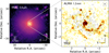 |
Fig. 1. Left: early-type galaxy ESO 420-G13 imaged by Spitzer/IRAC in the 3.6 μm continuum. Right: ALMA resolves the cold dust continuum at 1.2 mm into several knots that define a spiral pattern (background map). The nuclear disc is also revealed in the VLT/VISIR warm dust continuum at 12.7 μm adjacent to the [Ne II]12.8μm emission line (black contours, starting from 2× RMS with a spacing of ×10N/3; Asmus et al. 2014). The nuclear point-like source is possibly associated with synchrotron emission from the AGN, also detected at radio frequencies (Condon et al. 1996, 1998). The synthesised beam size is shown in the upper right corner. |
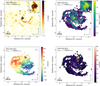 |
Fig. 2. ALMA maps of the 1.2 mm continuum (upper left), CO(2–1) intensity (upper right), CO(2–1) average velocity (lower left), and CO(2–1) average velocity dispersion (lower right) for the Seyfert 2 galaxy ESO 420-G13. The zoomed inset panels correspond to the grey square regions indicated in the corresponding maps. Contours in all panels correspond to the [Ne II]12.8μm line emission from VLT/VISIR (starting from 3× RMS with a spacing of ×10N/4). Assuming trailing spiral arms implies that the south-east extreme of the kinematic minor axis is the nearest point to us. The synthesised beam size is shown in the inset panels and in the upper right corner of the lower maps. |
2.3. Mid-infrared narrow-band imaging
ESO 420-G13 was imaged using the VISIR3 instrument, installed at the Very Large Telescope on Cerro Paranal (Chile) during the night of 19 January 2006 (programme ID: 076.B-0696). These observations include two narrow-band filters in the N band, NEII (λc = 12.81 μm, Δλ = 0.21 μm) and NEII_2 (λc = 13.04 μm Δλ = 0.22 μm), which were acquired using a chopping throw of 10″ and a pixel scale of  . The final reduced images, processed using the VISIR pipeline delivered by ESO4 as described in Asmus et al. (2014), were taken directly from the SubArcSecond Mid-InfRared Atlas of Local AGN (SASMIRALA5). At a redshift of z = 0.01205, the NEII_2 filter contains the [Ne II]12.8μm fine-structure line redshifted to 12.96 μm, while the adjacent NEII filter provides a measurement of the ∼12.5–12.7 μm mid-IR continuum in the rest frame. Because the two narrow-band filters have a similar width and transmission, we directly subtracted the continuum image from the line image. The difference in transmission between the two filters is of the order of the photometric error, that is, about 5% as measured for the associated calibrators in the SASMIRALA atlas. The lack of reference stars in the VISIR FOV means that a reliable astrometric calibration for the mid-IR images could not be obtained. Therefore, we assumed that the position of the bright mid-IR nucleus is coincident with that of the compact nuclear continuum source in the ALMA 1.2 mm map.
3. Results
At first sight, ESO 420-G13 resembles an early-type galaxy in the Spitzer/IRAC 3.6 μm image (left panel in Fig. 1). An inner kiloparsec-sized disc is revealed by both warm and cold dust emission (right panel). The superior angular resolution of ALMA allows us to resolve the dust emission at 1.2 mm into three main components: a circumnuclear ring with  diameter (190 pc), an unresolved point-like source in the centre of this ring, and a kiloparsec-sized spiral structure. The latter is more prominent in the CO(2–1) intensity map (upper right panel in Fig. 2), where the cold molecular gas can be traced at radii up to ∼1.1 kpc away from the nucleus. The inner ring is presumably located at the inner Lindblad resonance, showing bright CO(2–1) emission likely associated with active star formation. This is also the case for the bright 1.2 mm continuum spot in the north-east, which has enhanced molecular gas emission as well. Inside the ring we detect diffuse line emission, but the lack of a bright knot in CO(2–1) is in contrast with the bright core found in the 1.2 mm continuum at the centre of the ring (∼0.30 ± 0.08 mJy). This suggests that the millimetre radio emission from the nucleus could be non-thermal synchrotron radiation associated with the active nucleus. In this regard, a bright compact radio core was previously detected at 1.4 GHz by Condon et al. (1996), although at lower angular resolution (17″). Further radio observations at high-angular resolution would be required to probe the inner jet morphology and the synchrotron nature of the emission. The total CO(2–1) intensity integrated in the ALMA map is 260 ± 2 Jy km s−1, which corresponds to a mass of Mtot = (3.07 ± 0.02)×108 M⊙, assuming optically thick gas and α = 0.8 M⊙ (K km s−1 pc2)−1, as in LIRG and ULIRG galaxies (Bolatto et al. 2013). This is in agreement with the upper limit of < 109 M⊙ derived from previous single-dish observations (Elfhag et al. 1996). Faint CS(5–4) emission is detected in the nucleus (1.3 ± 0.2 Jy km s−1) and tentatively also in two molecular gas clumps in the spiral arms with integrated fluxes in the 0.3–0.5 Jy km s−1 range.
3.1. A Molecular gas wind
A remarkable wind has been detected through its redshifted CO(2–1) emission that extends along the kinematic minor axis of ESO 420-G13, within the inner kiloparsec of the galaxy. It can be clearly distinguished in the mean velocity and sigma moment maps obtained from the spectral cube that we show in the lower panels of Fig. 2. The wind extends from  to
to  away from the nucleus (340 pc to 600 pc) with projected velocities in the +50–250 km s−1 range, and presumably indicates the orientation of the central engine axis. Its locus with respect to the systemic velocity (3568 ± 7 km s−1, this work) can be seen in the cube slices from 115 to 190 km s−1 shown in Fig. 3. The channel map reveals a characteristic funnel shape morphology (e.g. Privon et al. 2008; Wagner & Bicknell 2011), with a narrow filamentary emission starting at
  ,
,  (340 pc projected distance), at 115 km s−1, elongated in the outflow direction, prior to a bifurcation point. The latter is probed by a bright spot in CO(2–1) emission at 130 and 145 km s−1, located at
  ,
,  relative to the 1.2 mm continuum nucleus (pink marker in Fig. 3; 440 pc projected distance). At this forking point, the wind starts spreading farther out perpendicular to the direction of motion, developing a complex structure formed by filaments and several individual clouds that move faster along the cone axis and also with increasing distance from the nucleus. The width of the cone, measured in the direction perpendicular to the kinematic minor axis, ranges from the size of a beam or individual cloud (∼20 pc) up to 200 pc in its widest point. This morphology is also traced by the sigma map in Fig. 2 (σ ∼ 50 km s−1).
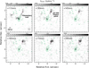 |
Fig. 3. CO(2–1) channel maps from +115 km s−1 to +190 km s−1 (step of 15 km s−1; projected velocities) relative to a systemic velocity of vsys = 3568 ± 7 km s−1 (this work). A complex filamentary emission in a gradually denser ISM is revealed within the outflowing wind, starting with a diffuse emission trail at |


To determine the position angle (PA) of the kinematic major and minor axes, we have modelled the galaxy rotation of the CO(2–1) gas using DISKFIT6 (Sellwood & Spekkens 2015). This code applies a χ2 minimisation to find a global model that fits the circular speed of the disc measured at different radii. In order to avoid over-fitting of non-axisymmetric components, only the rotation was considered here, thus radial flows or non-circular motions were not included in the fit. Furthermore, we fixed the axis ratio at b/a = 0.96 (from the NED7 based on 2MASS images). The best-fit model has a PA  for the kinematic major axis, and a systemic velocity8 of vsys = 3568 ± 7 km s−1. The rotation curve obtained is shown in the position-velocity (PV) diagram in Fig. 4 (pink line in the top panel). The molecular gas motions within the innermost
  (95 pc) appear to be dominated by a nuclear ring or disc that coincides with the ring observed in both the dust continuum and the CO(2–1) intensity distribution (see insets in Fig. 2). Outside of the ring, the velocities drop by ∼50 km s−1 from
  to 1″ at both sides of the major axis, as shown by the upper panel in Fig. 4, to increase again up to 80–100 km s−1 at
  from the nucleus. This is also evident in the mean velocity map in Fig. 2. The secondary maxima in velocity occur at the intersection of the PV cuts along the major axis with the spiral arms, suggesting that streaming motions associated with the density waves in the galaxy disc alter the local velocity field in these regions.
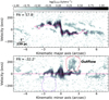 |
Fig. 4. Top: position-velocity diagram along the kinematic major axis (PA |


The spectral profile of the total integrated CO(2–1) emission shown in Fig. 5 (upper panel) is dominated by the galaxy rotation, which contributes more to the intensity in the blue side of the profile. The outflow contributes little to the integrated intensity (≲3%), while it is easily identified in the slice of the CO(2–1) datacube along the kinematic minor axis (bottom panel in Fig. 4). The wind can be seen in the spectrum of a short slice extracted along the kinematic minor axis (1″ < Δx < 3″; dot-dashed orange line in Fig. 5, bottom left panel), although the slit intersects only a small section of the outflow cone (see slit positions in the right panel of Fig. 5). Thus, the amplitude of the extracted spectrum is comparable to the interferometric artefacts in the map (see the negative residual at blueshifted velocities). An optimal extraction of the outflow spectrum can be performed using a 3D mask in the ALMA datacube, to select the outflow region in the spatial dimensions and isolate the wind from the rotating gas in the velocity dimension. The red contours in Figs. 4 and 5 represent the different projections of the 3D mask on the PV diagram and the image plane, while the integrated spectrum is shown in Fig. 5 (solid red line). No counter outflow is detected at the blueshifted side of the kinematic minor axis (−3″ < Δx < −1″; dashed blue line in Fig. 5) or in the integrated spectrum of the opposite symmetric 3D mask (dashed purple line). See Sect. 4 for a further discussion of this issue.
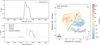 |
Fig. 5. Upper left: spectrum of the total integrated CO(2–1) emission for ESO 420-G13. Bottom left: spectra of the integrated flux for two pseudo-slits extracted along the kinematic minor axis, one intersecting the outflow (1″ < Δx < 3″, orange dot-dashed line) and one in the opposite direction (−3″ < Δx < −1″, dotted blue line). The CO(2–1) flux extracted from a 3D mask applied to the ALMA datacube allows us to isolate the outflow emission (solid red line) from the rotating gas. A symmetric mask located south-east of the nucleus at blueshifted velocities has also been applied, although no counter-outflow is detected in the integrated spectrum (dashed purple line). The negative amplitudes at ∼−70 km s−1 are produced by interferometric artefacts in the image reconstruction process. Right: pseudo-slit positions (dashed blue and dot-dashed orange rectangles) and the projections of the outflow mask (solid red contour) and the counter-outflow mask (dashed purple contour) are indicated in the mean velocity map. |
The integrated wind emission (7.0 ± 0.6 Jy km s−1) translates into a molecular gas mass of (8.3 ± 0.7)×106 M⊙, derived from the Solomon et al. (1997) formula and α = 0.8 M⊙ (K km s−1 pc2)−1, typical of LIRG and ULIRG galaxies (Bolatto et al. 2013). As no information on the excitation and optical depth of the gas in the wind is available, it is unclear whether other α values, such as those found for IC 5063 (Dasyra et al. 2016), could be appropriate. If instead a Milky Way value of α = 4.3 M⊙ (K km s−1 pc2)−1 is assumed (Bolatto et al. 2013), the derived mass would be significantly higher (4.5 ± 0.4)×107 M⊙. For the case of optically thin emission, the wind mass would drop by a factor of ∼3 (e.g. Combes et al. 2013; Dasyra et al. 2016).
3.2. Extended ionised gas
The [Ne II]12.8 μm emission-line contours above 3× RMS are over-plotted on the moment maps in Fig. 2 and the channel maps in Fig. 3. The ionised gas distribution shows a central peak likely associated with the AGN, plus an elongated plume with an extension of about 1″ (240 pc) towards the north-west direction, coincident with the kinematic minor axis. The orientation of the ionised gas emission is surprisingly well aligned with that of the CO(2–1) outflow, as is best seen in the 115 km s−1 velocity slice, for example (upper left panel in Fig. 3). The Spitzer/IRS spectrum obtained by Lebouteiller et al. (2015) suggests that the continuum filter is not affected by contamination from PAH or blueshifted [Ne II]12.8μm emission (see Fig. B.1).
At scales larger than the 3 × 3 kpc2 covered by the ALMA observations, ESO 420-G13 presents an extended tail of ionised gas towards the north-east and possibly the south-west, produced by the AGN and the star formation (Thomas et al. 2017). The far-IR lines observed by Herschel/PACS (Fernández-Ontiveros et al. 2016) show a brighter distribution along the kinematic minor axis (e.g. see the [O I]63 μm, the [O III]88 μm, and the [C II]158 μm maps in Fig. C.1). The lower angular resolution in the far-IR ( per spaxel versus
  seeing in the optical) does not explain this difference. No dust lanes that could explain this displacement are detected in the IRAC (Fig. 1) or the 2MASS archival images. A more efficient cooling of the diffuse rarefied gas through the far-IR lines (Osterbrock & Ferland 2006) needs to be examined using observations at higher angular resolution.
4. Discussion
4.1. A wind revealing a jet
The results shown in Sect. 3 indicate the detection of a jet-related wind in ESO 420-G13, that is, of a collimated outflow oriented along the minor axis of the galaxy and powered by the mechanical energy input from the AGN. In this picture, we interpret the extended [Ne II]12.8 μm emission as a collimated ionised wind associated with hot gas in the jet cavity. The structure of the molecular gas outflow farther out closely resembles that of numerical simulations of jet-cloud interactions (Wagner & Bicknell 2011; Wagner et al. 2016). The jet percolates the porous ISM, propagating through a tenuous medium until it collides with a denser molecular core and splits, leading to the apparent bifurcation. Fig. 3 shows a collimated filamentary outflow starting at a projected distance of 340 pc from the nucleus and at relatively low velocities (115 km s−1). At higher velocities, the outflow obtains a conical shape, with a starting point that is most likely associated with a dense jet-ISM impact point at 440 pc. The exterior of the dispersed gas cone has lower projected velocities than the interior of the cone, which can be explained if, for instance, part of the jet remains in its initial trajectory. The dispersed gas also moves faster (160–290 km s−1; Fig. 3) with increasing distance from the impact point, which can be explained if the energy is mainly transported near the jet front. Inversely, the narrow side of the cone shows a relatively high velocity dispersion (≳50 km s−1) when compared to the gas rotation (∼20 km s−1), which could be explained by the effect of higher turbulence (Wagner et al. 2012) or higher ram pressure (in the case of a two-phase medium; Hopkins & Elvis 2010) in the clouds that first experienced the jet impact. Overall, overpressured jets can inflate a bubble within the ISM, bifurcate, and cause conical winds and disperse the molecular gas into several clumps and filaments (Wagner et al. 2012). This picture is similar to that seen in the galaxy IC 5063 (Dasyra et al. 2016).
The cases of NGC 1377 and ESO 420-G13 suggest that unresolved jets might still have an important role in the feeding process even for weak radio galaxies. Unresolved jets have been increasingly detected in Seyfert galaxies (Baldi et al. 2018). In NGC 1377 (Aalto et al. 2016), no radio emission was known at the time that the molecular wind was detected. In ESO 420-G13, faint radio emission was seen, but its origin could not be linked to a jet. The molecular wind suggests the presence of a jet, which was most likely unresolved in previous radio observations (< 17″; Condon et al. 1996, 1998). Overall, elusive jets like those seen in NGC 1377 or ESO 420-G13 can be detected through their interaction with the ISM. While in NGC 1377 a continuous outflow can be traced from the nucleus up to a distance of 150 pc at both sides along the jet axis, in ESO 420-G13, the molecular gas wind starts at 340 pc away from the nucleus, which could further strengthen the argument that a jet is present. At shorter radii the molecular gas shows regular rotation, while the morphology of the [Ne II]12.8 μm emission suggests that an ionised wind might be present in the innermost few hundred parsecs. Future integral field spectroscopic observations at subarcsecond resolution would be required to confirm the nature of the ionised wind. No counter-outflow is detected in the opposite direction of the redshifted molecular gas outflow. In the following subsection, we propose geometries that could explain the jet-cloud interactions.
4.2. Jet-cloud configuration
Two main scenarios are explored to explain how the observed outflow could be driven by jet-cloud interactions. First, we consider a jet close to the galaxy minor axis that collides with a cloud located far from the galaxy plane. The non-detection of a blueshifted counterpart is reasonable because the likelihood of finding a molecular cloud at a relatively high altitude is low. The existence of such a cloud could even require out-of-equilibrium dynamical conditions, caused by a previous feedback episode or by a minor merger in the past, for instance. A previous outflow event could have been launched by supernovae (SNe), by the AGN radiation, or by former jet activity, as in the case of Centaurus A (Salomé et al. 2016), for example. In this scenario, the molecular gas would have re-formed as the relic outflow cooled down (Richings & Faucher-Giguère 2018). Thus, the current jet event could push the same material farther away that was ejected in the past. Alternatively, the minor merger scenario could be supported by the high IR luminosity in ESO 420-G13 (∼1011 L⊙) and the post-starburst features reported by Thomas et al. (2017) in the optical spectrum. This could also explain the existence of molecular gas clouds at a high altitude above the disc and the non-symmetric distribution of clouds on the opposite side. However, no stellar emission in the IRAC 3.6 μm associated with the minor companion has been detected (see left panel in Fig. 1). With the current dataset, we deem a past feedback event more likely than a past minor merger event.
In the second scenario, the jet is pushing molecular gas that belongs to the (thick) galaxy disc, at an intrinsically low altitude. For a jet moving nearly parallel to the disc as a result of precession, as in the case of IC 5063, the jet does not really shatter until it hits a dense molecular core at 340 pc. At shorter radii, the jet percolates the ISM through the inner circumnuclear ring, leading to the [Ne II]12.8 μm emission in the low-density cavities. However, the outflow asymmetry is hard to justify. Alternatively, a jet emerging perpendicular to the galaxy disc might be considered, which then bents or precesses at a certain height and is redirected towards the disc. This would explain why the innermost gas is unaffected. The [Ne II]12.8 μm emission in this case would also be associated with the low-density ionised medium cone that is carved out by the jet in the ISM. The one-sided wind would require an asymmetric bending of the jet, which is often observed in radio galaxies. However, the jet-bending region is not identified in the CO(2–1) or the [Ne II]12.8 μm line maps. If the jet bending were caused by precession, the symmetric counter-jet would likely have generated a blueshifted outflow because the disc is rich in molecular gas near the expected impact point. If the jet bending were linked to a collision with a molecular cloud, then this cloud would be small or destroyed and, thus, non-detectable.
4.3. Energy and momentum balance
Another argument favouring the jet scenario comes from the comparison of the wind kinetic luminosity and the radio power of ESO 420-G13. The wind kinetic luminosity (Lkin) was computed from the product  , where M is the mass of the gas in the wind, V is the wind speed measured as the average speed of the outflow spectrum in Fig. 5 (160 km s−1, projected velocity), and d is the distance from the location of the driving mechanism. For a radio jet, this is equivalent to the jet-cloud impact point. In our computations, we always assume that the wind started away from the nucleus, not that it was transported from the nucleus to ∼340 pc away. If the jet-ISM interaction occurs near the forking point of the outflowing CO(2–1) emission (Fig. 3), then the average projected distance covered by the wind is d ∼ 100 pc (
 ). For an outflow mass of (8.3 ± 0.7)×106 M⊙ (see Sect. 3.1), we derive a mass outflow rate of Ṁ ∼MV/d = 14 ± 1 M⊙ yr−1, a kinetic luminosity of Lkin = 1.1 × 1041 erg s−1, and a momentum rate of the accelerated gas of ṀV = 1.4 × 1034 erg cm−1. The error in the mass outflow rate corresponds only to the propagated uncertainty of the CO(2–1) intensity measurement, while a larger uncertainty is expected from the assumed geometry and the adopted α value. Furthermore, these values should be considered as lower limits because of the projection effect. If an inclination angle of i ∼ 20°–30° is assumed, then the deprojected velocity would be about 320–470 km s−1, and the corresponding kinetic luminosity would be ∼4–9 × 1041 erg s−1. We did not include the velocity dispersion to define the average velocity of the wind, as has been done in Fluetsch et al. (2019), for example. Although this approach may be appropriate for a spherical wind, given the high collimation in our case, we consider that including the turbulence of the wind would overestimate its average velocity.
We first compare these quantities with the kinetic and radiative power of the active nucleus in ESO 420-G13. In order to compute the radio power, we used two different methods that provide lower and upper limits. The lower limit was derived by fitting the radio-to-IR spectral energy distribution (SED), compiled from NED in the 843 MHz to 70 μm range (Fig. 6; Table A.1). The dust component was fitted using a modified black body (Casey 2012). Assuming that the synchrotron radiation from the nucleus dominates at low frequencies, this component was modelled using a broken power law with an exponential cut off (Rybicky & Lightman 2004), which is in agreement with the ALMA fluxes for the radio core (open circles in Fig. 6, not included in the fit). With a standard χ2 minimisation method, a minimum radio power of 1039 erg s−1 was found. The jet power, as computed from its radio emission, could be missing some of the energy deposited in a hot bubble that does pdV work. An estimate of the total mechanical power is obtained from the calibration by Heckman & Best (2014) for a sample of ∼40 radio galaxies by comparing the derived values of the work required to inflate the X-ray cavities observed in these galaxies with the monochromatic 1.4 GHz continuum flux of the nucleus (data from Cavagnolo et al. 2010; Bîrzan et al. 2008; and Rafferty et al. 2006). Following Heckman & Best (2014), we used a normalisation factor of fcav = 4, and a 1.4 GHz flux of 65 mJy (Condon et al. 1998; Table A.1) to estimate a total mechanical power of ∼4 × 1042 erg s−1 in ESO 420-G13. Therefore, the radio power differs from the wind kinetic luminosity by up to an order of magnitude, despite the wide range in the estimated jet power.
 |
Fig. 6. Flux distribution of the radio-to-IR continuum emission for ESO 420-G13 compiled from the literature (black circles). Our ALMA continuum measurements at 227 GHz and 241 GHz for the nuclear point-like source ( |


For a SMBH mass of MBH ∼ 4×10⁸ M⊙ (see Sect. 1) and an AGN luminosity of LAGN = 0.5–1 × 1044 erg s−1, that is, 10–20% of the total IR luminosity based on the flux ratios of the mid-IR fine-structure lines observed by Spitzer/IRS ([Ne V]14.3μm/[Ne II]12.8μm = 0.10 ± 0.01 and [O IV]25.9 μm/[Ne II]12.8 μm = 0.45 ± 0.03; Fernández-Ontiveros et al. 2016), the corresponding Eddington ratio is log(LAGN/Ledd)≲ − 2.7. This suggests that the active nucleus is likely in the radio or kinetic mode, thus favouring the jet scenario. Notably, ESO 420-G13 is not classified as radio loud according to classical IR-to-radio flux ratios integrated over the whole galaxy (qIR = 2.7, radio-loud galaxies have qIR ≲ 1.8; Ivison et al. 2010). If we were to consider the AGN contribution alone, the qIR to values would lie in the 1.7–2.0 range, which would mean that the nucleus would be very close to the radio-loud domain if the radio emission were dominated by the AGN. Higher angular resolution observations (< 1″) at radio wavelengths are required to probe the jet morphology and constrain its power estimate.
4.4. Other wind drivers
The question remains whether the wind is triggered by AGN radiation. The AGN emission accounts only for ∼10–20% of the galaxy bolometric luminosity, that is, LAGN = 0.5–1 × 1044 erg s−1. This is more than three orders of magnitude higher than the X-ray luminosity, which might instead be dominated by star formation in the host galaxy (see Sect. 1). If the wind were driven by radiation pressure from the AGN, its distance from the generating mechanism would be higher than before, that is, ∼600 pc ( ). Thus, the wind mass flow rate and momentum rate would be 2.3 M⊙ yr−1 and 2.3 × 1033 erg cm−1. This momentum rate does not exclude the AGN as a potential driving mechanism, considering the estimated radiation pressure of LAGN/c = 1.7–3.7 × 1033 erg cm−1 and the momentum boosting that can be achieved during some phases of energy-driven expansion (Cicone et al. 2014). Still, in this scenario it would be hard to explain why the molecular gas rotating close to the nucleus is not blown away.
Regarding the radiation pressure from stars, no clear sign of a local starburst such as excess emission in the dust continuum is detected near the outflow region. No significant excess of hot dust can be claimed in the 12.8 μm continuum image either. Rather weak emission is seen in the 1.2 mm continuum map (see the upper left panel in Fig. 2) that originates from three discrete knots in or near the area that the CO wind occupies. These regions all have comparable fluxes in the 0.11–0.15 mJy range and contribute up to a total of 0.48 ± 0.08 mJy. Even if all of the pertinent emission were to originate from the cold dust instead of the jet-related synchrotron, none of these regions could produce more than 2.5% of the total cold dust emission, which is equal to 6.1 ± 0.3 mJy. The corresponding IR luminosity fraction is 2 × 10⁹ L⊙ (as LIR for the entire galaxy is 8 × 10¹⁰ L⊙). Following Kennicutt (1998), this translates into a local SFR of 0.3 M⊙ yr−1. Given that ∼100 M⊙ are needed for one SN event to take place, the probability is very low for a SN to be responsible for this wind. Alternatively, a population of (young) stars cannot drive the wind either. The area comprising the CO wind occupies 4% of the overall galaxy in the near-IR (JHKs 2MASS bands). The overall galaxy emission, which is comparable in the IR and in the optical bands and includes the AGN contribution, is (5.8 ± 1.3)×1044 erg s−1. The force exerted on the gas through stellar radiation pressure, Lstars/c, would then be as high as 7.7 × 1032 erg cm−1, which is significantly lower than the momentum rate of the gas (1.4 × 1034 erg cm−1). Therefore, neither SNe nor stellar radiation can locally drive the wind.
Kinetic luminosity carried away by the molecular gas wind in ESO 420-G13, compared to different possible launching mechanisms, i.e. AGN radiation, jet power, and star formation.
4.5. Further evolution of ESO 420-G13
For a mass outflow rate of 14 M⊙ yr−1 and a total molecular gas mass of Mtot = (3.07 ± 0.02)×108 M⊙ (see Sect. 3), the depletion time would be of η = Mtot/Ṁ = 23 Myr at the current outflow rate. However, the outflowing gas would likely not escape the galaxy, falling again to the central part. Therefore, the result of this interaction points to a delay of the star formation and not to a quenching, while most of the feedback effect is expected in the central few hundred parsecs of the galaxy. This is in line with the results from Fluetsch et al. (2019). More violent AGN activity in the past would be required in order to explain the current evolutionary stage of ESO 420-G13.
5. Summary
We presented a collimated molecular gas outflow detected in the CO(2–1) transition using ALMA interferometric observations of the central 3 × 3 kpc2 in the Seyfert 2 galaxy ESO 420-G13. The molecular gas outflow has a conical shape with a width of ∼20 pc at the closest point to the nucleus and up to 200 pc at the farthest point. It carries a molecular gas mass of ∼8 × 10⁶ M⊙ yr−1 at an average projected velocity of 160 km s−1, which translates into an outflow rate of ∼14 M⊙ yr−1. Based on the outflow structure and the energy and momentum balance, we conclude that this is a jet-driven wind powered by mechanical energy input from the AGN. This is the second case after NGC 1377 in which a previously unknown jet is revealed through its interaction with the ISM. However, in ESO 420-G13 the molecular gas wind is detected very far from the AGN, at 340 pc (projected), traced only by [Ne II]12.8 μm ionised gas emission at closer distances down to the nucleus. Two possible scenarios were proposed to explain the origin of such an outflow: (i) an outer molecular cloud originated by previous jet activity or a minor merger event, then impacted by the current jet, or (ii) a molecular cloud in the galaxy disc impacted by a jet that propagates through the porous ISM after a bending or a precession. The outflowing molecular gas we detected will likely fall back into the galaxy, which will delay and not quench the star-forming process in the centre.
The case of ESO 420-G13 proves that moderate-luminosity jets in weak radio galaxies can still play a main role in driving molecular gas outflows in these objects. Deep and high-angular resolution data for CO lines, radio wavelengths, and ionised gas are required to reveal these jets. In this context, the TWIST survey will provide a census of similar jet-driven outflows in nearby galaxies, allowing us to move from individual galaxy studies to a robust statistical analysis of these phenomena.
Flat ΛCDM, H0 = 73 km s−1 Mpc−1, and Ωm = 0.27, z = 0.01205 (this work).
VLT spectrometer and imager for the mid-infrared (Lagage et al. 2004).
European Southern Observatory.
The NASA/IPAC Extragalactic Database (NED) is operated by the Jet Propulsion Laboratory, California Institute of Technology, under contract with the National Aeronautics and Space Administration.
Relativistic velocity, defined in the kinematic local standard of rest frame (LSRK).
Acknowledgments
The authors acknowledge the referee for his/her useful comments that helped to improve the manuscript. JAFO acknowledges financial support by the Agenzia Spaziale Italiana (ASI) under the research contract 2018-31-HH.0. JAFO and KMD acknowledge financial support by the Hellenic Foundation for Research and Innovation (HFRI), under the first call for the creation of research groups by postdoctoral researchers that was launched by the General Secretariat For Research and Technology (project number 1882). MPS acknowledges support from the Comunidad de Madrid, Spain, through Atracción de Talento Investigador Grant 2018-T1/TIC-11035 and STFC through grants ST/N000919/1 and ST/N002717/1. CR acknowledges support from the CONICYT+PAI, Convocatoria Nacional subvención a instalación en la academia, convocatoria año 2017 PAI77170080. This paper makes use of the following ALMA data: ADS/JAO.ALMA#2017.1.00236.S. ALMA is a partnership of ESO (representing its member states), NSF (USA) and NINS (Japan), together with NRC (Canada), MOST and ASIAA (Taiwan), and KASI (Republic of Korea), in cooperation with the Republic of Chile. The Joint ALMA Observatory is operated by ESO, AUI/NRAO and NAOJ. The National Radio Astronomy Observatory is a facility of the National Science Foundation operated under cooperative agreement by Associated Universities, Inc.
References
- Aalto, S., Muller, S., Sakamoto, K., et al. 2012, A&A, 546, A68 [NASA ADS] [CrossRef] [EDP Sciences] [Google Scholar]
- Aalto, S., Costagliola, F., Muller, S., et al. 2016, A&A, 590, A73 [NASA ADS] [CrossRef] [EDP Sciences] [Google Scholar]
- Alatalo, K., Blitz, L., Young, L. M., et al. 2011, ApJ, 735, 88 [NASA ADS] [CrossRef] [Google Scholar]
- Alonso-Herrero, A., Pereira-Santaella, M., García-Burillo, S., et al. 2018, ApJ, 859, 144 [Google Scholar]
- Armus, L., Bernard-Salas, J., Spoon, H. W. W., et al. 2006, ApJ, 640, 204 [NASA ADS] [CrossRef] [Google Scholar]
- Asmus, D., Hönig, S. F., Gandhi, P., Smette, A., & Duschl, W. J. 2014, MNRAS, 439, 1648 [NASA ADS] [CrossRef] [Google Scholar]
- Baldi, R. D., Williams, D. R. A., McHardy, I. M., et al. 2018, MNRAS, 476, 3478 [NASA ADS] [CrossRef] [Google Scholar]
- Bîrzan, L., McNamara, B. R., Nulsen, P. E. J., Carilli, C. L., & Wise, M. W. 2008, ApJ, 686, 859 [NASA ADS] [CrossRef] [Google Scholar]
- Bolatto, A. D., Wolfire, M., & Leroy, A. K. 2013, ARA&A, 51, 207 [Google Scholar]
- Bower, R. G., Benson, A. J., Malbon, R., et al. 2006, MNRAS, 370, 645 [NASA ADS] [CrossRef] [Google Scholar]
- Casey, C. M. 2012, MNRAS, 425, 3094 [Google Scholar]
- Cavagnolo, K. W., McNamara, B. R., Nulsen, P. E. J., et al. 2010, ApJ, 720, 1066 [NASA ADS] [CrossRef] [Google Scholar]
- Choi, E., Ostriker, J. P., Naab, T., Oser, L., & Moster, B. P. 2015, MNRAS, 449, 4105 [NASA ADS] [CrossRef] [Google Scholar]
- Cicone, C., Feruglio, C., Maiolino, R., et al. 2012, A&A, 543, A99 [NASA ADS] [CrossRef] [EDP Sciences] [Google Scholar]
- Cicone, C., Maiolino, R., Sturm, E., et al. 2014, A&A, 562, A21 [NASA ADS] [CrossRef] [EDP Sciences] [Google Scholar]
- Cicone, C., Severgnini, P., Papadopoulos, P. P., et al. 2018, ApJ, 863, 143 [NASA ADS] [CrossRef] [Google Scholar]
- Combes, F., García-Burillo, S., Casasola, V., et al. 2013, A&A, 558, A124 [NASA ADS] [CrossRef] [EDP Sciences] [Google Scholar]
- Condon, J. J., Helou, G., Sanders, D. B., & Soifer, B. T. 1996, ApJS, 103, 81 [NASA ADS] [CrossRef] [Google Scholar]
- Condon, J. J., Cotton, W. D., Greisen, E. W., et al. 1998, AJ, 115, 1693 [NASA ADS] [CrossRef] [Google Scholar]
- Croton, D. J., Springel, V., White, S. D. M., et al. 2006, MNRAS, 365, 11 [NASA ADS] [CrossRef] [Google Scholar]
- Dasyra, K. M., Combes, F., Novak, G. S., et al. 2014, A&A, 565, A46 [NASA ADS] [CrossRef] [EDP Sciences] [Google Scholar]
- Dasyra, K. M., Combes, F., Oosterloo, T., et al. 2016, A&A, 595, L7 [NASA ADS] [CrossRef] [EDP Sciences] [Google Scholar]
- De Looze, I., Cormier, D., Lebouteiller, V., et al. 2014, A&A, 568, A62 [NASA ADS] [CrossRef] [EDP Sciences] [Google Scholar]
- Diamond-Stanic, A. M., & Rieke, G. H. 2012, ApJ, 746, 168 [Google Scholar]
- Dubois, Y., Gavazzi, R., Peirani, S., & Silk, J. 2013, MNRAS, 433, 3297 [NASA ADS] [CrossRef] [Google Scholar]
- Elfhag, T., Booth, R. S., Hoeglund, B., Johansson, L. E. B., & Sandqvist, A. 1996, A&AS, 115, 439 [NASA ADS] [Google Scholar]
- Fabian, A. C. 2012, ARA&A, 50, 455 [NASA ADS] [CrossRef] [Google Scholar]
- Fernández-Ontiveros, J. A., Spinoglio, L., Pereira-Santaella, M., et al. 2016, ApJS, 226, 19 [NASA ADS] [CrossRef] [Google Scholar]
- Feruglio, C., Maiolino, R., Piconcelli, E., et al. 2010, A&A, 518, L155 [NASA ADS] [CrossRef] [EDP Sciences] [Google Scholar]
- Feruglio, C., Fiore, F., Maiolino, R., et al. 2013, A&A, 549, A51 [NASA ADS] [CrossRef] [EDP Sciences] [Google Scholar]
- Feruglio, C., Fabbiano, G., Bischetti, M., et al. 2019, ApJ, submitted [arXiv:1904.01483] [Google Scholar]
- Fiore, F., Feruglio, C., Shankar, F., et al. 2017, A&A, 601, A143 [NASA ADS] [CrossRef] [EDP Sciences] [Google Scholar]
- Fluetsch, A., Maiolino, R., Carniani, S., et al. 2019, MNRAS, 483, 4586 [NASA ADS] [Google Scholar]
- García-Burillo, S., Combes, F., Usero, A., et al. 2014, A&A, 567, A125 [NASA ADS] [CrossRef] [EDP Sciences] [Google Scholar]
- García-Burillo, S., Combes, F., Usero, A., et al. 2015, A&A, 580, A35 [NASA ADS] [CrossRef] [EDP Sciences] [Google Scholar]
- Goulding, A. D., & Alexander, D. M. 2009, MNRAS, 398, 1165 [NASA ADS] [CrossRef] [Google Scholar]
- Heckman, T. M., & Best, P. N. 2014, ARA&A, 52, 589 [Google Scholar]
- Hopkins, P. F., & Elvis, M. 2010, MNRAS, 401, 7 [NASA ADS] [CrossRef] [Google Scholar]
- Ivison, R. J., Alexander, D. M., Biggs, A. D., et al. 2010, MNRAS, 402, 245 [NASA ADS] [CrossRef] [Google Scholar]
- Kennicutt, Jr., R. C. 1998, ApJ, 498, 541 [NASA ADS] [CrossRef] [Google Scholar]
- Kormendy, J., & Ho, L. C. 2013, ARA&A, 51, 511 [Google Scholar]
- Lagage, P. O., Pel, J. W., Authier, M., et al. 2004, The Messenger, 117, 12 [NASA ADS] [Google Scholar]
- Lebouteiller, V., Barry, D. J., Goes, C., et al. 2015, ApJS, 218, 21 [NASA ADS] [CrossRef] [Google Scholar]
- Makarov, D., Prugniel, P., Terekhova, N., Courtois, H., & Vauglin, I. 2014, A&A, 570, A13 [CrossRef] [EDP Sciences] [Google Scholar]
- Morganti, R., Oosterloo, T., Oonk, J. B. R., Frieswijk, W., & Tadhunter, C. 2015, A&A, 580, A1 [NASA ADS] [CrossRef] [EDP Sciences] [Google Scholar]
- Nyland, K., Alatalo, K., Wrobel, J. M., et al. 2013, ApJ, 779, 173 [NASA ADS] [CrossRef] [Google Scholar]
- Osterbrock, D. E., & Ferland, G. J. 2006, Astrophysics Of Gaseous Nebulae And Active Galactic Nuclei (University Science Books) [Google Scholar]
- Privon, G. C., O’Dea, C. P., Baum, S. A., et al. 2008, ApJS, 175, 423 [NASA ADS] [CrossRef] [Google Scholar]
- Rafferty, D. A., McNamara, B. R., Nulsen, P. E. J., & Wise, M. W. 2006, ApJ, 652, 216 [NASA ADS] [CrossRef] [Google Scholar]
- Richings, A. J., & Faucher-Giguère, C.-A. 2018, MNRAS, 474, 3673 [Google Scholar]
- Rosario, D. J., Togi, A., Burtscher, L., et al. 2019, ApJ, 875, L8 [Google Scholar]
- Rush, B., Malkan, M. A., & Spinoglio, L. 1993, ApJS, 89, 1 [NASA ADS] [CrossRef] [Google Scholar]
- Rybicky, G., & Lightman, A. P. 2004, Radiative Processes in Astrophysics (Weinheim: Wiley-VCH Verlag GmbH Co. KGaA) [Google Scholar]
- Salomé, Q., Salomé, P., Combes, F., & Hamer, S. 2016, A&A, 595, A65 [NASA ADS] [CrossRef] [EDP Sciences] [Google Scholar]
- Sanders, D. B., Mazzarella, J. M., Kim, D.-C., Surace, J. A., & Soifer, B. T. 2003, AJ, 126, 1607 [Google Scholar]
- Sargsyan, L., Samsonyan, A., Lebouteiller, V., et al. 2014, ApJ, 790, 15 [NASA ADS] [CrossRef] [Google Scholar]
- Sellwood, J. A., & Spekkens, K. 2015 [arXiv:1509.07120] [Google Scholar]
- Silk, J., & Mamon, G. A. 2012, Res. Astron. Astrophys., 12, 917 [NASA ADS] [CrossRef] [Google Scholar]
- Solomon, P. M., Downes, D., Radford, S. J. E., & Barrett, J. W. 1997, ApJ, 478, 144 [NASA ADS] [CrossRef] [Google Scholar]
- Somerville, R. S., & Davé, R. 2015, ARA&A, 53, 51 [NASA ADS] [CrossRef] [EDP Sciences] [Google Scholar]
- Spoon, H. W. W., Farrah, D., Lebouteiller, V., et al. 2013, ApJ, 775, 127 [NASA ADS] [CrossRef] [Google Scholar]
- Springel, V., Di Matteo, T., & Hernquist, L. 2005, ApJ, 620, L79 [NASA ADS] [CrossRef] [Google Scholar]
- Stierwalt, S., Armus, L., Charmandaris, V., et al. 2014, ApJ, 790, 124 [NASA ADS] [CrossRef] [Google Scholar]
- Thomas, A. D., Dopita, M. A., Shastri, P., et al. 2017, ApJS, 232, 11 [NASA ADS] [CrossRef] [Google Scholar]
- Torres-Albà, N., Iwasawa, K., Díaz-Santos, T., et al. 2018, A&A, 620, A140 [NASA ADS] [CrossRef] [EDP Sciences] [Google Scholar]
- Wagner, A. Y., & Bicknell, G. V. 2011, ApJ, 728, 29 [NASA ADS] [CrossRef] [Google Scholar]
- Wagner, A. Y., Bicknell, G. V., & Umemura, M. 2012, ApJ, 757, 136 [NASA ADS] [CrossRef] [Google Scholar]
- Wagner, A. Y., Bicknell, G. V., Umemura, M., Sutherland, R. S., & Silk, J. 2016, Astron. Nachr., 337, 167 [NASA ADS] [CrossRef] [Google Scholar]
- Weedman, D. W., Hao, L., Higdon, S. J. U., et al. 2005, ApJ, 633, 706 [NASA ADS] [CrossRef] [Google Scholar]
- Weinberger, R., Springel, V., Pakmor, R., et al. 2018, MNRAS, 479, 4056 [NASA ADS] [CrossRef] [Google Scholar]
Appendix A: Radio to far-IR continuum fluxes
Far-IR to radio continuum fluxes for the nucleus of ESO 420-G13.
Appendix B: Transmission of VISIR narrow-band filters
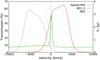 |
Fig. B.1. Transmission profile of the VISIR narrow-band filters NEII (grey line) and NEII_2 (orange line). The Spitzer/IRS high-resolution spectrum from Lebouteiller et al. (2015) suggests that contamination from PAH emission is not present within the inner kiloparsec (solid green line, right axis). A blueshifted emission line with −1000 km s−1 (dotted vertical line) would find the same transmission in both narrow-band filters, and therefore would not appear in the continuum-subtracted map. |
Appendix C: Optical versus far-IR fine-structure lines
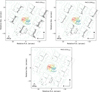 |
Fig. C.1. ALMA CO(2-1) mean velocity map is compared to the extended [O III]5007 Å line emission (green contours), the Herschel/PACS IFU spectra for the [O I]63 μm far-IR fine-structure line (square insets in the upper left panel), the [O III]88μm line (upper right panel), and the [C II]158μm line (lower panel). The optical datacube was taken from the Siding Spring Southern Seyfert Spectroscopic Snapshot Survey (Thomas et al. 2017) and was aligned to the ALMA data assuming that the peak of the stellar optical continuum coincides with the unresolved 1.2 mm radio core. As shown by Thomas et al. (2017), the [O III]5007 Å emission morphology is asymmetric and extended along PA ∼30°. Note the lower angular resolution of the PACS data ( |

All Tables
Kinetic luminosity carried away by the molecular gas wind in ESO 420-G13, compared to different possible launching mechanisms, i.e. AGN radiation, jet power, and star formation.
All Figures
|
Fig. 1. Left: early-type galaxy ESO 420-G13 imaged by Spitzer/IRAC in the 3.6 μm continuum. Right: ALMA resolves the cold dust continuum at 1.2 mm into several knots that define a spiral pattern (background map). The nuclear disc is also revealed in the VLT/VISIR warm dust continuum at 12.7 μm adjacent to the [Ne II]12.8μm emission line (black contours, starting from 2× RMS with a spacing of ×10N/3; Asmus et al. 2014). The nuclear point-like source is possibly associated with synchrotron emission from the AGN, also detected at radio frequencies (Condon et al. 1996, 1998). The synthesised beam size is shown in the upper right corner. |
| In the text | |
|
Fig. 2. ALMA maps of the 1.2 mm continuum (upper left), CO(2–1) intensity (upper right), CO(2–1) average velocity (lower left), and CO(2–1) average velocity dispersion (lower right) for the Seyfert 2 galaxy ESO 420-G13. The zoomed inset panels correspond to the grey square regions indicated in the corresponding maps. Contours in all panels correspond to the [Ne II]12.8μm line emission from VLT/VISIR (starting from 3× RMS with a spacing of ×10N/4). Assuming trailing spiral arms implies that the south-east extreme of the kinematic minor axis is the nearest point to us. The synthesised beam size is shown in the inset panels and in the upper right corner of the lower maps. |
| In the text | |
|
Fig. 3. CO(2–1) channel maps from +115 km s−1 to +190 km s−1 (step of 15 km s−1; projected velocities) relative to a systemic velocity of vsys = 3568 ± 7 km s−1 (this work). A complex filamentary emission in a gradually denser ISM is revealed within the outflowing wind, starting with a diffuse emission trail at |
| In the text | |
|
Fig. 4. Top: position-velocity diagram along the kinematic major axis (PA |
| In the text | |
|
Fig. 5. Upper left: spectrum of the total integrated CO(2–1) emission for ESO 420-G13. Bottom left: spectra of the integrated flux for two pseudo-slits extracted along the kinematic minor axis, one intersecting the outflow (1″ < Δx < 3″, orange dot-dashed line) and one in the opposite direction (−3″ < Δx < −1″, dotted blue line). The CO(2–1) flux extracted from a 3D mask applied to the ALMA datacube allows us to isolate the outflow emission (solid red line) from the rotating gas. A symmetric mask located south-east of the nucleus at blueshifted velocities has also been applied, although no counter-outflow is detected in the integrated spectrum (dashed purple line). The negative amplitudes at ∼−70 km s−1 are produced by interferometric artefacts in the image reconstruction process. Right: pseudo-slit positions (dashed blue and dot-dashed orange rectangles) and the projections of the outflow mask (solid red contour) and the counter-outflow mask (dashed purple contour) are indicated in the mean velocity map. |
| In the text | |
|
Fig. 6. Flux distribution of the radio-to-IR continuum emission for ESO 420-G13 compiled from the literature (black circles). Our ALMA continuum measurements at 227 GHz and 241 GHz for the nuclear point-like source ( |
| In the text | |
|
Fig. B.1. Transmission profile of the VISIR narrow-band filters NEII (grey line) and NEII_2 (orange line). The Spitzer/IRS high-resolution spectrum from Lebouteiller et al. (2015) suggests that contamination from PAH emission is not present within the inner kiloparsec (solid green line, right axis). A blueshifted emission line with −1000 km s−1 (dotted vertical line) would find the same transmission in both narrow-band filters, and therefore would not appear in the continuum-subtracted map. |
| In the text | |
|
Fig. C.1. ALMA CO(2-1) mean velocity map is compared to the extended [O III]5007 Å line emission (green contours), the Herschel/PACS IFU spectra for the [O I]63 μm far-IR fine-structure line (square insets in the upper left panel), the [O III]88μm line (upper right panel), and the [C II]158μm line (lower panel). The optical datacube was taken from the Siding Spring Southern Seyfert Spectroscopic Snapshot Survey (Thomas et al. 2017) and was aligned to the ALMA data assuming that the peak of the stellar optical continuum coincides with the unresolved 1.2 mm radio core. As shown by Thomas et al. (2017), the [O III]5007 Å emission morphology is asymmetric and extended along PA ∼30°. Note the lower angular resolution of the PACS data ( |
| In the text | |
Current usage metrics show cumulative count of Article Views (full-text article views including HTML views, PDF and ePub downloads, according to the available data) and Abstracts Views on Vision4Press platform.
Data correspond to usage on the plateform after 2015. The current usage metrics is available 48-96 hours after online publication and is updated daily on week days.
Initial download of the metrics may take a while.