| Issue |
A&A
Volume 633, January 2020
|
|
|---|---|---|
| Article Number | A54 | |
| Number of page(s) | 17 | |
| Section | Interstellar and circumstellar matter | |
| DOI | https://doi.org/10.1051/0004-6361/201936531 | |
| Published online | 10 January 2020 | |
The first steps of interstellar phosphorus chemistry★,★★
1
Center for Astrochemical Studies, Max-Planck-Institut für extraterrestrische Physik,
Gießenbachstraße 1,
85748 Garching, Germany
e-mail: chantzos@mpe.mpg.de
2
INAF – Osservatorio Astrofisico di Arcetri,
Largo Enrico Fermi 5,
50125
Firenze,
Italy
3
Ural Federal University, Ekaterinburg,
Russia
4
Visiting Leading Researcher, Engineering Research Institute “Ventspils International Radio Astronomy Centre” of Ventspils University of Applied Sciences,
Inženieru 101,
Ventspils 3601,
Latvia
Received:
20
August
2019
Accepted:
28
October
2019
Context. Phosphorus-bearing species are essential to the formation of life on Earth, however they have barely been detected in the interstellar medium. In particular, towards star-forming regions only PN and PO have been identified so far. Since only a small number of detections of P-bearing molecules are available, their chemical formation pathways are not easy to constrain and are thus highly debatable. An important factor still missing in the chemical models is the initial elemental abundance of phosphorus, that is, the depletion level of P at the start of chemical models of dense clouds.
Aims. In order to overcome this problem, we study P-bearing species in diffuse and translucent clouds. In these objects phosphorus is expected to be mainly in the gas phase and therefore the elemental initial abundance needed in our chemical simulations corresponds to the cosmic one and is well constrained.
Methods. For the study of P-bearing chemistry we used an advanced chemical model. We updated and significantly extended the P-chemistry network based on chemical databases and previous literature. We performed single-pointing observations with the IRAM 30 m telescope in the 3 mm range towards the line of sight to the strong continuum source B0355+508 aiming for the (2–1) transitions of PN, PO, HCP, and CP. This line of sight incorporates five diffuse and/or translucent clouds.
Results. The (2–1) transitions of the PN, PO, HCP, and CP were not detected. We report high signal-to-noise-ratio detections of the (1–0) lines of 13CO, HNC, and CN along with a first detection of C34S towards this line of sight. We have attempted to reproduce the observations of HNC, CN, CS, and CO in every cloud with our model by applying typical physical conditions for diffuse or translucent clouds. We find that towards the densest clouds with vLSR = −10, − 17 km s−1 the best-fit model is given by the parameters (n(H), AV, Tgas) = (300 cm−3, 3 mag, 40 K).
Conclusions. According to our best-fit model, the most abundant P-bearing species are HCP and CP (~10−10). The molecules PN, PO, and PH3 also show relatively high predicted abundances of ~10−11. We show that the abundances of these species are sensitive to visual extinction, cosmic-ray ionization rate, and the diffusion-to-desorption energy ratio on dust grains. The production of P-bearing species is favored towards translucent rather than diffuse clouds, where the environment provides a stronger shielding from the interstellar radiation. Based on our improved model, we show that the (1–0) transitions of HCP, CP, PN, and PO are expected to be detectable with estimated intensities of up to ~200 mK.
Key words: astrochemistry / line: identification / molecular processes / ISM: molecules
The phosphorus chemical network and the reduced spectra are only available at the CDS via anonymous ftp to cdsarc.u-strasbg.fr (130.79.128.5) or via http://cdsarc.u-strasbg.fr/viz-bin/cat/J/A+A/633/A54
© J. Chantzos et al. 2020
 Open Access article, published by EDP Sciences, under the terms of the Creative Commons Attribution License (http://creativecommons.org/licenses/by/4.0), which permits unrestricted use, distribution, and reproduction in any medium, provided the original work is properly cited.
Open Access funding provided by Max Planck Society.
1 Introduction
Phosphorus is essential for biotic chemistry, since it is a fundamental component of many important biological molecules, such as nucleic acids and phospholipids. Phosphorus is therefore vital to life on Earth and can consequently play an important role in exoplanets (Schaefer & Fegley 2011). Despite its importance, the chemistry of P-bearing molecules is in its infancy and remains poorly understood. The aim of this work is to add an important missing piece to the puzzle: unveiling the first steps of P chemistry via observations and chemical simulations of simple P-bearing molecules in diffuse clouds.
The ion P+ was detected in several diffuse clouds by Jura & York (1978), where an elemental abundance of ~2 × 10⁻⁷ with a low P depletion factor of between approximately two and three was derived. However, a more recent study by Lebouteiller et al. (2006) showed that phosphorus remains mostly undepleted towards diffuse clouds. In addition, P has been identified towards dwarf and giant stars (Maas et al. 2017; Caffau et al. 2016), while detections of simple P-bearing molecules (PN, PO, HCP, CP, CCP, NCCP, PH3) have been done towards the circumstellar material of carbon- and oxygen-rich stars (Agúndez et al. 2007, 2014a,b; Tenenbaum et al. 2007; De Beck et al. 2013; Ziurys et al. 2018). The species PN and only very recently PO are the only P-bearing molecules to have been discovered towards dense star-forming regions (Turner & Bally 1987; Fontani et al. 2016, 2019; Rivilla et al. 2016; Lefloch et al. 2016; Mininni et al. 2018) and molecular clouds in the Galactic Center (Rivilla et al. 2018). The limited number of available observations hinders our understanding of the chemical pathways involved in P chemistry. The main uncertainty in P chemistry is the unknown depletion factor of P in molecular clouds. In general, chemical models of dark clouds start with the so-called “low-metal abundances”, where the elemental abundances of heavy elements (such as P, S, Fe, Mg) are reduced by orders ofmagnitude to reproduce molecular observations (e.g., Agúndez & Wakelam 2013), but with poor understanding of the chemical processes at the base of such depletions. In the case of P, the level of depletion is still very uncertain. While Turner et al. (1990) and Wakelam et al. (2015) used high depletion factors of 600–104 with respect to cosmic P abundance, recent works have shown that it could be as low as ~ 100 (Rivilla et al. 2016; Lefloch et al. 2016).
As only a very limited number of P-bearing molecules have been detected in star-forming regions, it is very hard to put constraints on the elemental abundance of P in the gas phase and on the major chemical pathways. In order to elucidate the interstellar P chemistry we focus on diffuse clouds, which represent the first steps of molecular-cloud evolution. Diffuse clouds can provide important constraints on P chemistry, since P in these objects is not strongly affected by depletion, meaning that the initial P abundance that can be used for chemical simulations is well constrained (Lebouteiller et al. 2006). With this approach we are able to remove an important uncertainty in our model and use a reliable starting point for our chemical simulations.
The existing chemical and physical models focus solely on diffuse clouds (e.g., Dalgarno 1988; Le Petit et al. 2004; Cecchi-Pestellini et al. 2012; Godard et al. 2014). For example, in Godard et al. (2014), a model including dissipation of turbulence was applied to reproduce the observed molecular abundances in the diffuse interstellar medium (ISM). The main results showed that chemical complexity is strongly linked to turbulent dissipation, which was able to reproduce the high abundances of CO and other species (such as C+ and HCO+) observed towards Galactic diffuse clouds. Le Petit et al. (2004) describe the development of a chemical model of the diffuse cloud towards ζ Persei that was able to reproduce the abundance of  and other species, like CN and CO. This was achieved by modeling two phases, namely a small dense phase (~ 100 au) with a density of n(H) = 2 × 104 cm−3 and a larger diffuse region (4 pc) with n(H) = 100 cm−3. In addition, the reproduction of the CH+ abundance and that of the rotationally excited H2 required the inclusion of shocks into the model. Similar results were achieved by Cecchi-Pestellini et al. (2012) when including the injection of hot H2 into the model.
Previous observations (Corby et al. 2018; Liszt et al. 2018; Thiel et al. 2019) prove the chemical complexity and the wide range of densities, temperatures, and visual extinctions of diffuse and translucent clouds, making them promising targets for observations of P-bearing molecules. Diffuse clouds are characterized by low densities with n(H) = 100−500 cm−3 and are therefore more exposed to interstellar radiation, which can destroy molecules. Translucent clouds on the other hand are an intermediate state between diffuse and dense molecular clouds, being more protected from UV radiation (1 mag < AV < 5 mag). They are denser with typical densities of n(H) = 500−5000 cm−3 and are consequently cooler (Tgas = 15−50 K), showing higher chemical complexity (Snow & McCall 2006; Thiel et al. 2019). One prominent candidate that has been widely studied in previous works (e.g., Liszt et al. 2018, and references therein) is the gas that lies along the line of sight to the compact extragalactic continuum source B0355+508. This strong blazar is located at a very low latitude in the outer Galaxy (b = −1.6037°), meaning that the way through the Galactic disk is long and therefore gathers a significant amount of distributed Galactic diffuse gas (Pety et al. 2008). Indeed, the line of sight towards B0355+508 shows a complex kinematic structure which incorporates several diffuse and translucent clouds. The detections of numerous molecules like S- and CN-bearing species as well as small hydrocarbons towards B0355+508 also indicate the rich chemistry present in this diffuse and translucent gas (e.g., Liszt et al. 2018, and references therein). The substantial velocity structure coupled with a high chemical complexity of this line of sight enables us to adjust our chemical and physical model to every cloud component and find which physical conditions most favor the abundances of P-bearing molecules. Other background sources that have previously been studied are either lacking the chemical (like B0224+671) or the velocity (such as B0415+479) features which are essential for the present work.
In this paper, we present single-pointing observations of the (2–1) transitions of HCP, CP, PN, and PO and chemical simulations of their molecular abundances towards the line of sight to B0355+508 in order to investigate P-bearing chemistry within diffuse and translucent clouds, the precursors of molecular clouds. In Sect. 2 we describe the observational details. Section 3 summarizes the results of the observations. In Sect. 4 we describe our updated phosphorus chemical network as well as the grid of models that we apply in order to reproduce the observations of HNC, CN, CS, and CO towards every cloud component along the line of sight. Furthermore, in Sect. 5 we focus on the P-bearing chemistry based on our best-fit model (which was determined in Sect. 4). In particular, we report the predicted molecular abundances of HCP, CP, PN, PO, and PH3 and we study their dependence on visual extinction, cosmic-ray ionization rate, and diffusion-to-desorption energy ratio on dust grains. A future outlook and conclusions are summarized in Sects. 6 and 7.
2 Observations
The observations of the HCP (2–1), CP (2–1), PN (2–1), and PO (2–1) transitions in the 3 mm range were carried out at the IRAM 30 m telescope located at Pico Veleta (Spain) towards the line of sight to the compact extragalactic quasar B0355+508. Table 1 lists the observed transitions, the spectroscopic constants, and the telescope settings at the targeted frequencies: the upper state energy is described by Eup, the upper state degeneracy is given by gu, while Aul stands for the Einstein coefficient of the transition u → l. The main beam efficiency and the main beam size of the telescope at a given frequency are denoted by the parameters Beff and θMB, respectively.For our observations we used the EMIR receiver with the E090 configuration (3 mm atmospheric window). We applied three observational setups, in which every setup covered a total spectral coverage of 7.2 GHz (each sub-band covered 1.8 GHz). As a backend we used the Fast Fourier Transform Spectrometer with a frequency resolution of 50 kHz (0.15 km s−1 at 100 GHz). In addition, we applied the wobbler switching mode with an amplitude offset of ± 90″. Pointing and focus of the telescope was performed every 2 h on the background source B0355+508 itself and was found to be accurate to within 2″.
The intensity of the obtained spectra was converted from antenna ( ) to main beam temperature (Tmb) units, using the following relation:
  , where Feff is the forward efficiency. Feff is equal to 95% in the targeted frequency range.
3 Results
The compact extragalactic source B0355+508 is located at α = 3h 59m 29.73s, δ = 50°57′50.2″ with a low galactic latitude of b = −1.6037°, incorporating a large amount of Galactic gas along the line of sight that harbors up to five diffuse and/or translucent clouds at velocities of −4, − 8, − 10, − 14 and −17 km s−1 (e.g., Liszt et al. 2018, and references therein). The flux of the blazar B0355+508 is variable over time and has been measured at ~ 3 mm to be on average equal to (4.62 ± 1.02) Jy, after averaging the flux of 76 different observations (Agudo 2017). This corresponds to a temperature Tc of (0.96 ± 0.21) K at a beam size of 27″ by taking into account the Rayleigh-Jeans-Approximation. The obtained spectra were reduced and analyzed by the GILDAS software (Pety 2005). Every detected line was fitted via the standard CLASS Gaussian fitting method. For the derivation of the peak opacity we use the radiative transfer equation
![\begin{eqnarray*}T_{\mathrm{mb}} &=& (J_{\nu}(T_{\mathrm{ex}})-J_{\nu}(T_{\mathrm{bg}}) - J_{\nu}(T_{\mathrm{c}}))\;{\times}\;(1-\exp{(-\tau)}) \Rightarrow \nonumber \\[2pt] \tau &=& -\ln \left(1 - \frac{T_{\mathrm{mb}}}{J_{\nu}(T_{\mathrm{ex}})-J_{\nu}(T_{\mathrm{bg}})-J_{\nu}(T_{\mathrm{c}})}\right), \end{eqnarray*}](/articles/aa/full_html/2020/01/aa36531-19/aa36531-19-eq4.png) (1)
(1)
where Tex is the excitation temperature, Tbg is the cosmic background temperature, and  describes the Rayleigh-Jeans temperature in Kelvin1. After obtaining the peak opacity τ, the column density N is then estimated by following the relation:
 (2)
(2)
with kB being the Boltzmann constant, Δv the line width (FWHM), ν the transition frequency, c the speed of light, and h the Planck constant. Qrot(Tex) gives the partition function of a molecule at a given excitation temperature Tex.
The (2–1) transitions of HCP, CP, PN, and PO were not detected within our observations (see Fig. 1). We derive 3σ upper limits for the opacities and column densities of the P-bearing species using Eqs. (1) and (2). Due to the low densities in diffuse clouds, molecules are expected to show no collisional excitation. The column densities were calculated assuming Tex = Tbg = 2.7 K, which simplifies Eq. (1) to:
 (3)
(3)
The results are summarized in Table 2.
We detected the HNC (1–0), CN (1–0), and C34S (2–1) transitions in absorption as well as the 13CO (1–0) in emission at the 3 mm range with a high signal-to-noise ratio (S/N), ranging from 6 to 802. Figure 2 shows all the detected spectra towards the line of sight to B0355+508. In the case of CN we were able to detect and resolve four hyperfine components from 113.123 to 113.191 GHz (see Fig. 3). Every hyperfine component was detected in the three velocity components at − 8, − 10, and − 17 km s−1 except for the one weak transition at 113.123 GHz, which was identified only in two clouds (at − 10, − 17 km s−1). The molecule HNC was identified in all five cloud components, while C34 S (in absorption) and 13 CO (in emission) were detected solely towards the densest features, at − 10 and − 17 km s−1. Table 3 lists the identified species and the corresponding spectroscopic parameters.
For estimating the CN column density we use the hyperfine component at 113.170 GHz. Our derived opacities and column densities of CN agree within a factor of two to three with previous results (Liszt & Lucas 2001), while the HNC results are well reproduced within a factor of 1.5. Table 4 summarizes the derived opacities and column densities of the detected species, as well as the obtained line intensities and rms levels.
Lucas & Liszt (2002) reported the detection of the main isotopolog C32S with the IRAM Plateau de Bure interferometer (PdBI) and estimated a column density of (4.27 ± 0.16) × 1012 cm−2 at the − 10 km s−1 component and (3.06 ± 0.32) × 1012 cm−2 at − 17 km s−1. With the above values and the column densities of C34S calculated in this work, we derive a sulfur isotopic ratio 32S∕34S of 12.8 ± 4.8 and 18.7 ± 9.5 for the components at − 10 and − 17 km s−1, respectively. The latter value is in good agreement with the 32S∕34S ratio for the local ISM of 24 ± 5 (Chin et al. 1996). However, the isotopic ratio determined for v = −10 km s−1 is significantly lower than the local interstellar value, which could be the result of opacity effects of the C32S line. In addition, the determination of the sulphur isotopic ratio was based on just one spectral line of the main species C32S and its isotopolog, which also yields a high uncertainty. To our knowledge this is the first detection of C34S towards this line of sight, owing to the high spectral resolution of ~50 kHz and high sensitivity (rms of ~4 mK) achieved with our observations.
In Liszt & Lucas (1998), detections of the main species 12CO and its isotopolog 13CO are reported, which were obtained with the PdBI as well as the NRAO 12 m telescope. The single-dish observations covered a large beam of 60′′, thus seeing CO and its isotopolog in emission, while the interferometric observations were sensitive only to the very narrow column of gas towards the strong background blazar, giving rise to absorption lines. For deriving the excitation temperatures and the column densities, both emission (single-dish data) and absorption lines (interferometric data) were considered.
In Fig. 2 it is clearly visible that the strong 13 CO emission line at − 10 km s−1 overlaps with an absorption feature at around − 8 km s−1. This is probably due to the fact that absorption is present close to the background source, meaning that emission and absorption lines are merged together in our observations with the IRAM 30 m telescope. This contamination effect is influencing the line profile at − 10 km s−1 which subsequently results in an unreliable fit. This could possibly explain why the 13 CO column density derived at − 10 km s−1 deviates by a factor of about four from previous results (Liszt & Lucas 1998), while towards − 17 km s−1, N(13CO) is well reproduced within 10% (see Table 4)3. Our derived isotopic ratio 12CO∕13CO at − 17 km s−1 is equal to 16.7 ± 1.4. For this calculation, we used the column density of 12CO derived in Liszt & Lucas (1998) with N(12CO) = (6.64 ± 0.47) × 1015 cm−2. The resulting CO isotopic ratio is almost a factor of four lower than the local interstellar ratio 12 C∕13C = 60 (Lucas & Liszt 1998). This was already confirmed by previous studies (Liszt 2007, 2017) that show an increased insertion of 13 C into CO towards clouds in the translucent regime with elevated densities and/or smaller radiation fields, which lead to an enhanced abundance of 13CO by a factor of two to four. Under these conditions isotope exchange fractionation (13 C+ + 12CO →12C+ + 13CO + 35 K) is more dominant than selective photodissociation.
Spectroscopic parameters of the observed species and telescope settings.
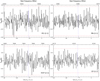 |
Fig. 1 Spectra of the nondetected (2–1) transitions of PO, PN, HCP, and CP. The upper x-axis shows the rest frequency (in MHz) and the lower one is a velocity axis (in km s−1). The red dashed line indicates the 3σ level and the blue dashed line shows the transition frequency of the corresponding molecule. In the case of PO, we show as an example one of the observed transitions at 108.998 GHz. |
Derived upper limits for the opacity and the column density of HCP, CP, PN, and PO.
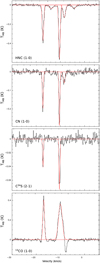 |
Fig. 2 Spectra of the detected species HNC, CN, C34S, and 13 CO in the 3 mmrange towards the line of sight to the extragalactitc source B0355+508. The red line represents the CLASS Gaussian fit. |
 |
Fig. 3 Detected hyperfine components of the CN (1–0) transition between 113.12 and 113.20 GHz. The three strongest hyperfine components were detected in the three clouds with vLSR =−8, − 10, − 17 km s−1 except for the one weak transition (N, F) = (1, 1∕2) - (0, 1∕2), which was identified only in the two densest clouds (at − 10, − 17 km s−1). |
Spectroscopic parameters of the detected species and telescope settings.
Gaussian fitting results of CN, HNC, C34S, 13 CO.
4 Chemical modeling
The goal of the present study is to constrain and improve our model of diffuse and translucent clouds to make reliable predictions regarding the abundances of P-bearing species (and also others). For this reason, we used the observations of HNC, CN, CS, and CO in order to constrain the physical parameters in our model. The chemical code that we applied was developed by Vasyunin & Herbst (2013) with an updated grain-surface chemistry (Vasyunin et al., in prep.). The model includes a gas-grain chemical network with 6000 gas-phase reactions, 200 surface reactions, and 660 species. Accretion and desorption processes regulate and connect the gas-phase and grain surface chemistry. The code numerically solves coupled differential equations (chemical rate equations) and computes a set of time-dependent molecular abundances. Since the observations were carried out towards diffuse and translucent clouds, we considered as initial elemental abundances the standard Solar elemental composition (see Table 5). We note that our initial elemental abundances are significantly different compared to the low metal abundances used in Wakelam et al. (2015) for dark clouds (200 times more abundant S and up to 104 more abundant Fe, Cl, P, and F). In particular, the initial abundance of P is 2.6 × 10⁻⁷ and is therefore well constrained unlike in dense molecular clouds. This approach will help us better elucidate the chemistry ofP since a key parameter for the chemical model is well determined. In addition, we begin our chemical simulations with the entirety of hydrogen being in its atomic form in order to start with pure atomic diffuse cloud conditions.
4.1 The chemical network of phosphorus
The phosphorus chemical network that has been used in previous studies (Fontani et al. 2016; Rivilla et al. 2016) has been extended with new available information in the literature (new reactions, updated reaction rates, desorption energies, etc.). In particular, chemical reactions of several P-bearing species, such as PN, PO, HCP, CP, and PH3, were included and/or updated in our chemical network. The reaction rates were taken from the online chemical databases KInetic Database for Astrochemistry (Wakelam et al. 2015, KIDA)4 and the UMIST Database for Astrochemistry (McElroy et al. 2013, UDfA)5, as well as from numerous previous papers (Thorne et al. 1984; Adams et al. 1990; Millar 1991; Anicich 1993; Charnley & Millar 1994; Jiménez-Serra et al. 2018). In particular we included several reactions involving the formation and destruction of PHn (n = 1, 2, 3) and their cationic species from Charnley & Millar (1994) and Anicich (1993), along with the chemical network proposed by Thorne et al. (1984) that contains production and loss routes for P, PO, P+, PO+, PH+, HPO+ and H2 PO+. In addition, weextended the PN chemical network based on the work by Millar et al. (1987), and we took into account the gas-phase reaction P + OH → PO + H proposed byJiménez-Serra et al. (2018), as well as two formation routes of PN in the gas phase, N +CP → PN + C and P + CN → PN + C, by Agúndez et al. (2007). Finally, we included the photodissociation reactions of PN, PO, HCP, and PHn (n = 1, 2, 3) based on the reaction rates given in KIDA and UDfA. The reaction rates of the photodissociation of PHn were assumed to be equal to the analogous reactions for NHn.
Concerning the chemistry taking place on grain surfaces, we took into account the hydrogenation reactions of P-bearing species (where the letter “g” denotes a grain surface species) as well as their corresponding desorption reactions:
-
gH + gP → gPH,
-
gH + gPH → gPH2,
-
gH + gPH2 → gPH3.
The desorption energy of PH3 was calculated based on that of NH3 and amounts to ~ 5800 K. This corresponds to an evaporation temperature of ~100 K, which is in good agreement with the value of ~90 K proposed by Turner et al. (1990)6. The reactive desorption efficiency in our chemical model is set equal to 1%. An increased reactive desorption of 10% changes the predicted abundances of the aforementioned P-bearing molecules by less than a factor of two. Another nonthermal desorption mechanism included in our model is the cosmic-ray desorption, which is fully described in Hasegawa & Herbst (1993). Based on this study, dust grains are heated upon impact with cosmic rays reaching a peak temperature Tdust of 70 K, which subsequently leads to preferential desorption of molecules from grain surfaces. This type of desorption is however negligible in diffuse clouds, where photodesorption dominates. In our model we adopt for all species a photodesorption rate of 3 × 10⁻³ molecules per incident UV photon, as was determined in Öberg et al. (2007) based on laboratory measurements of pure CO ice. This stands in good agreement with the photodesorption yield of ~ 10−3 molecules per UV photon found for other species, such as H2O, O2 and CH4 (Öberg et al. 2009; Fayolle et al. 2013; Dupuy et al. 2017).
Assumed solar initial elemental abundances (Asplund et al. 2006).
4.2 Comparison to observations
In order to reproduce the observed abundances of HNC, CN, CS, and CO in every cloud towards the line of sight to B0355+508 we produce a grid of models applying typical physical conditions for diffuse or translucent gas (Snow & McCall 2006; Thiel et al. 2019). We note here that, since our chemical model is not treating isotopic species, we are using as a reference for our comparison the main species 12CO and C32 S instead of 13CO and C34S. For the fractional abundances of 12CO and C32S, we are adopting the column densities determined in Liszt & Lucas (1998) and Lucas & Liszt (2002). In addition, for the clouds at − 14 and − 4 km s−1 we use for CN and CS the upper limits derived in this work (N(CN) < 1012 cm−2) and in Lucas & Liszt (2002). The parameter space that we investigate is listed below:
-
n(H) = 100−1000 cm−3, spacing of 100 cm−3,
-
AV = 1−5 mag, spacing of 1 mag,
-
Tgas = 20−100 K, spacing of 10 K.
The chemical evolution in each model is simulated over 107 yr (100 time steps) assuming static physical conditions. For the cosmic-ray ionization rate ζ(CR) we use a value of 1.7 × 10⁻¹⁶ s−1 (Indriolo & McCall 2012, see Sect. 5 for further explanation). This also corresponds to the values applied in Godard et al. (2014) and Le Petit et al. (2004), where the best-fit models provided a ζ(CR) of 10−16 s−1 and 2.5 × 10⁻¹⁶ s−1, respectively.
Given the above parameter space, we calculate the level of disagreement D(t, r) between modeled and observed abundances (for the species HNC, CN, CS and CO), which, following Wakelam et al. (2010) and Vasyunin et al. (2017), we define as
 (4)
(4)
with r = (n(H), AV, Tgas) and  is the observed or modeled abundance of species j, respectively. We then determine the minimal value of D(t, r), (noted as Dmin(t, r)), that corresponds to the best-fit model; the parameters (t, r) provided by the best-fit model are the ones giving the smallest deviation between observations and predictions. The smaller the Dmin(t, r), the better the agreement.
According to Pety et al. (2008) and references therein, the clouds with vLSR = −10 and − 17 km s−1 towards B0355+508 show strong 12 CO emission lines that originate from dense regions (with n(H) = 300−500 cm−3 and N(H2) > 1021 cm−2) which are just outside the synthesized beam (combination of the 30 m and PdBI telescopes), but still within the IRAM 30 m beam (Pety et al. 2008). Based on the CO (2–1) maps shown in Pety et al. (2008) with 22′′ and 5.8′′ resolutions, respectively, the cloud at vLSR = −10 km s−1 shows the most pronounced, dense substructure. This is confirmed by the fact that this particular cloud component produces the most detectable amounts of observed species in the data presented in this work and previous works by Liszt & Lucas (2001) and Lucas & Liszt (2000), and is therefore chemically the most complex one. The component at vLSR = −8 km s−1 shows a similar structure to the one at vLSR = −10 km s−1, incorporating a dense region as well. Pety et al. (2008) suggest that the two components are part of the same cloud, even though they are distinguishable in absorption and show different levels of chemical complexity. With a higher spatial resolution of 5.8′′, the CO emission at vLSR = −8 km s−1 is separated from the one at vLSR = −10 km s−1 and is clearly visible. The diffuse gas seen at velocities − 14 and − 4 km s−1 shows barely any 13 CO (Liszt & Lucas 1998, and this work) or 12CO (Pety et al. 2008; Liszt & Lucas 1998) in emission, which suggests that the density of these clouds is too low to sufficiently excite CO. Pety et al. (2008) estimated a low to moderate density of these clouds to be ~ 64−256 cm−3 with AV < 2 mag.
Since we are performing single-dish observations with a beam of ~ 22′′, we also cover the high-density regions that produce significant 12 CO emission (Pety et al. 2008). For this reason we constrain our grid of models to high densities of ≥ 300 cm−3 for the denser clouds (− 8, − 10, − 17 km s−1), while for the low-density objects at − 14 km s−1 and − 4 km s−1 we restrict our input parameters to n(H) ≤ 200 cm−3 and AV < 2 mag. The calculation of the molecular abundances was done with respect to the H2 column densities (N(H2) ~ 4−5 × 1020 cm−2) that were derived towards every cloud by Liszt et al. (2018). However, our model provides the fractional abundance of a species X with respect to the total number of hydrogen nuclei, as in n(X)∕n(H), with the total volume density of hydrogen defined as n(H) = n(H I + 2 × H2). The surface mobility parameters that we set as default values in our model (see Sect. 5.3) enable fast and effective formation of H2 on the surfaces of grains. At the end of our simulations (at t = 107 yr), the H2 abundance reaches a value of 40−50% (depending on the set of parameters). This means that almost the entire hydrogen is predicted to be in its molecular form at the late phases of the chemical evolution. Following this consideration, we divide all the observed abundances and their upper limits mentioned in this paper by a factor of two, since n(X)∕n(H I + 2 × H2) ≃ n(X)∕2 × n(H2) = 0.5 × n(X)∕n(H2). We note that this expression applies to the high-density parts of the clouds and does not account for the low-density (and H I rich) gas along the line of sight.
Figure 4 shows the results of the grid of models that was applied to reproduce the observations towards vLSR = −17 km s−1. In particular, we plot D(tbest, r), which describes the deviation between observed and modeled abundances at the time of best agreement tbest, versus the density, temperature, and visual extinction. Between an AV of 1 and 3 mag the smallest level of disagreement D(tbest, r) reduces by 13%. The main discrepancy between observed and modeled abundances at low AV comes from the fact that a high visual extinction results in higher molecular abundances and is therefore able to reproduce the chemical complexity seen towards the translucent clouds. For models with AV > 3 mag the minimal D(tbest, r) barely changes (less than 1% of increase). The smallest D(tbest, r) increases with respect to the density and temperature up to 3 and 2%, respectively. This is a clear indication that the most influential physical parameter in our analysis is the visual extinction.
For the cloud component at vLSR = −17 km s−1 the best-fit model with Dmin(t, r) is reached ata time tbest = 6.2 × 10⁶ yr and has the parameters: rbest = (n(H), AV, Tgas) = (300 cm−3, 3 mag, 40 K). At tbest = 6.2 × 10⁶ yr we also fulfill the assumption of having most of the hydrogen in molecular form, as the H2 abundance reaches a value of 0.45. Based on this model, we show in Fig. 5 the time dependent abundances of CO, CN, CS and HNC over 107 yr as well as the corresponding observed abundances towards vLSR = −17 km s−1. Our chemical model reproduces the observed species CO, CN, and CS very well within a factor of ~ 1−1.4 at tbest = 6.2 × 10⁶ yr. As can be seen in Fig. 5, the predicted abundances follow the order of the observed quantities. The most significant discrepancy is found in case of HNC, where the chemical model underestimates the observed abundance by a factor of four at the time of best agreement (see Table 6). According to the model, one of the main destruction mechanisms of HNC is: C+ + HNC → C2N+ + H; based on the online chemical databases, its reaction rate remains uncertain. In UDfA the given reaction rate was determined theoretically (Leung et al. 1984) and therefore entails a high uncertainty. Experimental studies of the above chemical route are still needed to make reliable predictions of the HNC abundance.
The smallest deviation with the observations towards the cloud with vLSR = −10 km s−1 was produced by the same set of parameters: rbest = (n(H), AV, Tgas) = (300 cm−3, 3 mag, 40 K). However, in this case the best-fit model gives a Dmin(t, r) that is slightly larger by a factor of approximately 1.4. The molecular abundances observed towards vLSR = −8 km s−1 are best reproduced with an AV of 5 mag, a density of 400 cm−3 and a gas temperature of 40 K. The smallest level of disagreement between an AV of 3 and 5 mag differs by less than 1%.
For the two remaining clouds with vLSR = −4 km s−1 and vLSR = −14 km s−1 the best-fit model in both cases is given by the parameters: (n(H), AV, Tgas) = (200 cm−3, 1 mag, 30 K) at tbest = 107 yr. Here, the discrepancy in both clouds arises mostly from the fact that the model underestimates the CS abundance by a factor of between approximately six and nine. In our model, CS is being effectively destroyed via photodissociation due to the low AV. Table 7 lists the best-fit parameters that were determined towards every cloud component.
We note that towards the same line of sight there have been detections of several other molecules, as reported in Liszt et al. (2008). The best-fit model determined towards vLSR = −17 km s−1 and vLSR = −10 km s−1 is able to reproduce within one order of magnitude the species OH, C2H, H2 CO, NH3 and CH, while other species such as HCN, SO, H2S and C3H2 are strongly underestimated by up to two orders of magnitude. This is a clear indication that the chemical network of certain molecules (other than P-bearing ones) still needs to be extended and updated. This however will be addressed in future work, as the present paper focuses mainly on P chemistry.
 |
Fig. 4 Results of the grid of models applying typical conditions for diffuse or translucent clouds in order to reproduce the observations towards the cloud at vLSR =−17 km s−1. The deviation between observations and model at the time of best agreement tbest is given by D(tbest, r), which is plotted versus density, temperature, and visual extinction. The best-fit model is given at a time tbest = 6.2 × 10⁶ yr and has the following parameters: (n(H), AV, Tgas) = (300 cm−3, 3 mag, 40 K). |
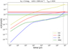 |
Fig. 5 Chemical evolution of the abundances of CO, CN, CS and HNC over 107 yr predicted by our best-fit model with the parameters (n(H), AV, Tgas) = (300 cm−3, 3 mag, 40 K). The colored horizontal bands correspond to the observed abundances towards the cloud with vLSR =−17 km s−1, including the inferred uncertainties. The vertical dashed line indicates the time of best agreement (t = 6.2 × 10⁶ yr) between observations and model results. |
Observed abundances for the cloud component with vLSR = −17 km s−1 and predictions of the species HNC, CO, CS, and CN based on our best-fit model at the time of best agreement t = 6.2 × 10⁶ yr.
Set of physical parameters that give the best agreement between model results and observations towards every cloud component.
5 Discussion: the chemistry of phosphorus
Based on the above results we can conclude that the molecular abundances observed at vLSR = −8, − 10, − 17 km s−1 can be best reproduced by a more “shielded” (AV > 1 mag) interstellar medium that allows the build-up of molecules to occur more efficiently. The resulting visual extinction AV of 3 mag should be viewed as an average value over the region covered by our beam (~ 22′′). Within this region the denser clumps are most likely translucent in nature. Hence, the observed cloud components are probably heterogeneous clouds, incorporating diffuse and translucent material, filled with relatively abundant molecules. This result stands in good agreement with a study by Liszt (2017), which involved modeling the CO formation and fractionation towards diffuse clouds. One of the main results of this latter study was that strong 13 CO absorption lines observed in the millimeter- and UV-range can be explained by higher densities (≥ 256 cm−3) and weaker radiation (and thus higher visual extinction), as already mentioned in Sect. 3. Our conclusions also agree well with the work done by Thiel et al. (2019) in which the physical and chemical structure of the gas along the line of sight to SgrB2(N) was studied; here, complex organic molecules such as NH2CHO and CH3CHO were detected in the majority of the clouds, which at the same time proved to have relatively high visual extinctions (AV = 2.5−5 mag with N(H2) > 1021 cm−2), thus consisting mainly of translucent gas. According to Thiel et al. (2019) the column density of H2 that corresponds to an AV of 3 mag is ~3 × 1021 cm−2. This is also consistent with the study by Pety et al. (2008), which states that the bright 12 CO emission originates from dense regions with N(H2) > 1021 cm−2. The gas observed at velocities of − 14 and − 4 km s−1 on the other hand, corresponds mainly to a “classical” diffuse cloud with a visual extinction of ~ 1 mag according to the above analysis. These clouds also yielded the smallest amounts of the detected molecular abundances. Since chemical complexity seems to be favored towards translucent rather than diffuse gas, for the following discussion we use the model that provided the best fit towards the dense clouds with vLSR = −17 km s−1 and vLSR = −10 km s−1 as a reference.
According to our best-fit model, P+ has a gas-phase abundance of 1.8 × 10⁻⁷ at the end of our simulations, being a factor of approximately 1.4 lower than its cosmic value, which indicates that little depletion takes place. The main reservoir of phosphorus other than P+ is atomic P, having an abundance of 7.4 × 10⁻⁸ at 107 yr. Atomic P is formed mainly through the electronic recombination of P+. For our models with elevated densities (103 cm−3) we reach high elemental depletion (such as for C+, S+ and P+) after running the code for 107 yr. This is consistent with the results presented by Fuente et al. (2019), which show significant depletion of C, O, and S happening already towards translucent material at the edge of molecular clouds (3–10 mag) with 1− 5 × 103 cm−3. In Appendix A we investigate further the expected depletion of phosphorus when transitioning from diffuse- to dense-cloud conditions. We find that there is a significant depletion of atomic P on dust grains after the final density of 105 cm−3 is reached. This in turn leads to a strong increase of gPH3, that becomes the main carrier of phosphorus in the dense phase. We also find a considerable decrease of the molecules HCP, CP, PN, PO and PH3 due to freeze-out on grains and their destruction route with  after the final density is attained at t ~ 106−107 yr.
The most abundant P-bearing molecules in the gas phase are HCP and CP, with maximal abundances of 3.4 × 10⁻¹⁰ and 2.1 × 10⁻¹⁰, respectively7. The formation and destruction pathways of both HCP and CP are strongly related to the electron fraction, as they are mainly produced (throughout the entire chemical evolution) by dissociative recombination of the protonated species  and destroyed by reacting with C+, the main carrier of positive charge in diffuse clouds. Two additional P-bearing species that are predicted by our model to have “observable” abundances in the gas phase are PN and PO, with respective maximal abundances of 4.8 × 10⁻¹¹ and 1.4 × 10⁻¹¹. The most productive formation pathways for PN start with P + CN → PN + C, N + PH → PN + H and end with N + CP → PN + C. In the late stage of evolution (~ 0.5 × 10⁶ − 107 yr) PN is primarily being destroyed by He+ + PN → P+ + N + He. The species PO is mainly produced over the entire chemical evolution of 107 yr by the dissociative recombination of HPO+: HPO+ + e−→ PO + H, and is mostly destroyed by reactions with C+ and H+. On the other hand, HPO+ is efficiently formed via P+ + H2O → HPO+ + H8. An additional reaction that becomes relevant at progressive times (~ 106−107 yr) is O + PH → PO + H with a ~ 10% reaction significance.
Another relatively abundant P-bearing species in the gas-phase based on our best-fit model is phosphine, PH3, with a maximal abundance of ~1.6 × 10⁻¹¹ at a late time of 107 yr. We note here that the species PH is also predicted to be detectable with a maximal abundance of ~ 3.6 × 10⁻¹¹. Unlike PH however, PH3 has already been detected in circumstellar envelopes of evolved stars (Agúndez et al. 2014a), indicating that it could be an important P-bearing species in interstellar environments such as diffuse and translucent clouds. We therefore focus in the following sections on the PH3 rather than the PH chemistry. Based on our chemical model, PH3 is formed most efficiently on dust grains in the early phase, being released to the gas-phase via reactive desorption: gH + gPH2 → PH3. Its formation proceeds after 1.4 × 10³ yr with the photodesorption process gPH3 → PH3 being the most effective reaction. Since the evaporation temperature of PH3 lies at ~ 100 K, the main mechanism driving the desorption of PH3 at low temperatures is photodesorption (instead of thermal desorption). Switching off the photodesorption in our model leads to a decrease of the PH3 gas-phase abundance of two orders of magnitude. Once in the gas phase, PH3 is mostly destroyed by reactions with C+ and H+ as well as through the photodissociation reaction: PH3 + hν → PH2 + H. The most abundant species on grains is gPH3, with a maximal abundance of 7.2 × 10⁻¹⁰. Almost all the atomic P that depletes onto the dust grains reacts with gH and forms gPH (gP + gH → gPH), which subsequently forms gPH3 through further hydrogenation. Table 8 summarizes all the main formation and destruction pathways for the molecules PN, PO, HCP, CP and PH3 at three different times (t = 103, 105, 107 yr). The last column shows the significance of the given reaction in the total formation or destruction rate of the species of interest.
Figure 6 depicts the time-dependent abundances of PN, PO, HCP, CP and PH3 over 107 yr predicted by the best-fit model along with the computed 3σ upper limits. The predicted abundance for PO lies a factor of about 40 below the observational upper limit at t = 107 yr, while the current upper limits of HCP and CP are about one order of magnitude higher than the model predictions. Finally, for PN the modeled abundance almost reaches the observed value at the end of our simulations. This means that in all cases the predicted abundances of P-bearing species are lower than the derived upper limits. Future observations of the ground-energy transitions (1–0) will help us to constrain these upper limits even more (see Sect. 6 for further justification). Table 9 lists the predicted abundances of the above species given by our chemical model at t = 107 yr along with the corresponding upper limits. In the case of PO we show only the lowest value of the four upper limits that were derived for each transition.
In the following discussion we focus on how deviations from our best-fit model can affect the chemistry of P-bearing species. In particular, we examine the dependence of the abundances of HCP, CP, PN, PO and PH3 on increasing visual extinction AV, increasing cosmic-ray ionization rate ζ(CR), and alternating the surface mobility constants (diffusion-to-desorption ratio Eb ∕ED and possibility of quantum tunneling for light species).
5.1 Effects of visual extinction on the P-bearing chemistry
In this section, we analyze how an increase of AV is affecting the predicted abundances of P-bearing species. For this purpose we consider the parameters of the best-fit model with n(H) = 300 cm−3 and Tgas = 40 K, while varying the AV from 1 to 10 mag. By keeping the density constant, we avoid high levels of elemental depletion. The increase in visual extinction can then be explained by a figurative increase of the size of the source. Figure 7 (left panel) shows the predicted abundances of P-bearing species at the end of our simulations (t = 107 yr) under the effect of varying the visual extinction. All species reach a maximal abundance at an of 4 mag. The abundances of HCP, CP, and PN barely change for AV > 4 mag, while for the rest of the molecules the abundances drop; especially in the case of PH3 where we see a substantial decrease of almost two orders of magnitude. As already mentioned in Sect. 5, the most effective formation process of PH3 is the photodesorption gPH3 → PH3. Thus, a high visual extinction attenuates the incoming UV-field and therefore the desorption of gPH3.
In order to better understand the AV dependence of the remaining molecular abundances, we plotted in Fig. 7 the predicted abundances of the species that mainly form and destroy HCP, CP, PN, and PO (see Table 8) as a function of the visual extinction. In particular, we simulated the abundances of  , C+, P+, He+, and H+ as well as HPO+. In the case of HCP (and also CP) its abundance increases up to an AV of 4 mag and then remains constant above that value. This behavior is correlated with the increase of the
  abundance up to an AV of 3 mag as well as the decreaseof C+ up to a visual extinction of 4 mag. The species PO seems to be more strongly affected by the increasing AV. Its abundance will also increase for AV ≤ 4 mag which again stands in correlation with the decrease of the C+ abundance (the main “destroyer” of PO), followed by a drop in abundance up to 7 mag. This on the other hand results from the decrease in HPO+ abundance (the main precursor of PO) in the same AV range. An increase in AV will decrease the P+ abundance (due to the decrease of the total ionization rate), as can be seen in Fig. 7. In addition, an enhanced AV slightly decreases the H2O abundance (by a factor of two), since the most effective formation for H2 O at late times is the photodesorption gH2O → H2O (see footnote 7). Therefore, for higher AV, both P+ and H2 O decrease, meaning that HPO+ and subsequently PO reduce in abundance as well.
5.2 Effects of the cosmic-ray ionization rate on the chemistry of P-bearing species
As already mentioned in Sect. 4.2, for all the applied models we use a value of 1.7 × 10⁻¹⁶ s−1 for the cosmic-ray ionization rate ζ(CR), as was derived by Indriolo & McCall (2012). This is also consistent with previous work in which diffuse and translucent clouds were studied as well (Fuente et al. 2019; Godard et al. 2014; Le Petit et al. 2004). However, we should note here that in Indriolo & McCall (2012) several cosmic-ray ionization rates were derived towards 50 diffuse lines of sight, ranging from 1.7 × 10⁻¹⁶ to 10.6 × 10⁻¹⁶ s−1 with a mean value of 3.5 × 10⁻¹⁶ s−1. Due to the complex and not yet fully understood nature of our observed clouds, we test our chemical model by also applying the elevated values of ζ(CR) = 3.5 × 10⁻¹⁶ s−1 and 10.6 × 10⁻¹⁶ s−1 in order to examine the influence of the cosmic-ray ionization rate on P-bearing chemistry. As for the remaining parameters of the code (such as AV and Tgas) we use the values given by our best-fit model (see Sect. 4.2). Figure 8 shows the chemical evolution of the species PN, PO, HCP, CP and PH3 over 107 yr for ζ(CR) = 1.7 × 10⁻¹⁶ s−1 and 10.6 × 10⁻¹⁶ s−1 in the left and right panels, respectively.
Table 10 summarizes the predicted abundances of P-bearing species for the three different cosmic-ray ionization rates given in Indriolo & McCall (2012). As one can see that PN shows the most substantial decrease in abundance with increasing ζ(CR). From the lowest (ζ(CR) = 1.7 × 10⁻¹⁶ s−1) to the highest (ζ(CR) = 10.6 × 10⁻¹⁶ s−1) cosmic-ray ionization rate, the PN abundance decreases by a factor of approximately 730, while for HCP, CP, and PH3 we see a drop by a factor of about 85 and 50, respectively. As already mentioned, PN is heavily destroyed by He+ with a ~40% reaction significance. An increase of ζ(CR) up to a value of 10.6 × 10⁻¹⁶ s−1 significantly enhances the ionization of He and H by a factor of about 20 and 30, respectively, via cosmic-ray-induced secondary UV photons: He + CRP → He+ + e− and H + CRP → H+ + e− (the abundance of C+ increases by a factor of ~ 6). Therefore, the destruction path with H+ becomes relevant for all P-bearing species showing a 10–40% loss efficiency. The effect is the strongest in the case of PN, because PN is mainly formed through CP which drastically decreases and is also efficiently destroyed by both He+ and H+. The PO abundance is only reduced by a factor of about 20 after increasing ζ(CR) up to 10.6 × 10⁻¹⁶ s−1, despite being heavily destroyed by H+. On the other hand, the significance of the dissociative recombination of HPO+ increases up to 50% which in turn counterbalances the loss through H+. An increased ζ(CR) of 10.6 × 10⁻¹⁶ s−1 enhances the abundance of P+ up to ~2.5 × 10⁻⁷, nearly reaching its cosmic value of ~2.6 × 10⁻⁷ (Asplund et al. 2006), while the abundance of atomic P decreases down to ~ 9.5 × 10⁻⁹ via the enhanced reaction with C+ and H+.
Main formation and destruction mechanisms for the species PN, PO, HCP, CP, and PH3 based on the best-fit chemical model at times: t = 103, 105, 107 yr.
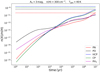 |
Fig. 6 Variation of the predicted abundances of PN, PO, HCP, CP and PH3 over 107 yr in our best-fit model. The dashed lines represent the 3σ upper limits derived from the observations at vLSR = −17 km s−1. In the case of PO we use 5 × 10⁻¹⁰ as an upper limit (see Table 9 and text for explanation). |
Observed and predicted abundances at time t = 107 yr for the species PO, PN, HCP, CP, and PH3 given by our best-fit model.
5.3 Effects of the diffusion-to-desorption ratio on the chemistry of P-bearing species
The chemistry in the ISM is heavily influenced by the presence of dust grains (Caselli & Ceccarelli 2012). The mobility of the depleted species on the surface of dust grains depends on two mechanisms: thermal hopping and quantum tunneling for the lightest species H and H2 through potential barriers between surface sites (Hasegawa et al. 1992). Without the possibility of tunneling, the species are not able to scan the grain surface quickly at low temperatures and the total mobility decreases. The parameters that strongly determine the surface chemistry are the diffusion-to-desorption energy ratio Eb ∕ED as well as the thickness of the potential barrier between adjacent sites. Based on previous studies (Hasegawa et al. 1992; Ruffle & Herbst 2000; Garrod & Herbst 2006), Vasyunin & Herbst (2013) proposed three different values for the Eb ∕ED ratio: 0.3, 0.5, and 0.77. In the case of low ratios (Eb∕ED = 0.3) we activate in our model the possibility of quantum tunneling for light species, while for the other two cases, surface mobility is only controlled by thermal hopping (and quantum tunneling is deactivated). The potential barriers are assumed to have rectangular shape and a thickness of 1 Å (Vasyunin & Herbst 2013). In our model we utilize the first set of parameters (Eb ∕ED = 0.3, with tunneling), nevertheless, since the chemistry of P-bearing species is still highly uncertain, we examine how the remaining two sets of parameters (Eb∕ED = 0.5, 0.77, no tunneling) influence the predicted abundances. Table 11 lists the predictions for PN, PO, HCP, CP, and PH3 as well as H2 at t = 107 yr for the three different sets of surface mobility parameters proposed in Vasyunin & Herbst (2013). As Table 11 shows, the H2 abundance decreases by a factor of four by switching from setup 1 (Eb∕ED = 0.3 with tunneling) to setup 2 (Eb∕ED = 0.5 no tunneling), and finally experiences a dramatic drop of a factor 50 when increasing the Eb ∕ED up to 0.77 (overall change of a factor 200 between setups 1 and 3).
The reduction of the H2 abundance has a significant impact on the formation of  and PH, which affects the PN, PO, HCP and CP abundances through the following reactions:
PN
-

-
-
N + PH → PN + H
PO
-
-

-
O + PH → PO + H
HCP


CP
Both PH and  decrease by a factor of approximately 20 when increasing the Eb∕ED up to 0.77. In addition, the abundance of H+ is increased by a factor of about 25, since the reduction of H2 formation leads to more atomic hydrogen and
subsequently more H+. The enhanced H+ abundance results in a stronger destruction of all P-bearing species through their reaction with H+. The species HCP and CP are also strongly affected by changing the surface mobility parameters, with an overall decrease by a factor of about 70 and 65 in abundance, respectively. In both cases the dissociative recombination of  is essential during the whole chemical evolution for the formation of HCP and CP showing a reaction significance of 30–99%. A decrease of
  due to lower H2 abundance therefore results in reduced HCP and CP formation. The largest effect is seen for PN, where a diffusion-to-desorption ratio of 0.77and no quantum tunneling of light species reduces the PN abundance by a factor of 300 (see Fig. 9).
Besides the effective loss through H+, the substantial decrease in PN is also related to the reduction of CP, which is the main precursor of PN at late times. In addition, the reaction N + PH → PN + H is important for PN formation over the entire chemical evolution of 107 yr with a 10–50% formation efficiency (for Eb∕ED = 0.77 and no tunneling). This means that the reduction of the H2 abundance decreases PH, which in turn produces less PN. In the case of PO however, the change in abundance between the two extreme cases is only a factor of about 20. Here, the route O +PH → PO + H increases in significance only up to 3% at late times (4 × 10⁶−107 yr), indicating that the decrease of PH will not considerably affect PO production. Furthermore, the reduction of PO due to H+ is compensated through its effective formation via the dissociative recombination of HPO+. Finally, the abundance of PH3 decreases only by a factor of 13 in total when changing the surface chemistry constants. Despite being heavily destroyed by H+, PH3 is still sufficiently formed through the photodesorption of gPH3.
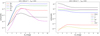 |
Fig. 7 Predicted abundances of P-bearing molecules as a function of visual extinction AV. The molecular abundances shown here are computed at t = 107 yr. Right panel: predicted abundances of |

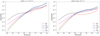 |
Fig. 8 Chemical evolution of P-bearing molecules as a function of time under the effects of cosmic-ray ionization rates of ζ(CR) = 1.7 × 10⁻¹⁶ s−1 (left panel) and 10.6 × 10⁻¹⁶ s−1 (right panel). |
Predicted abundances of the species PN, PO, HCP, CP, and PH3 at t = 107 yr for three different cosmic-ray ionization rates (see text for explanation).
Predicted abundances of the species PN, PO, HCP, CP, and PH3 as well as H2 at t = 107 yr for three different sets of surface mobility parameters (see text for explanation).
6 Future observations
Thanks to the sensitive observations (rms of ~6 mK) of the (2–1) transitions of HCP, CP, PN and PO we were able to obtain good upper limits for the column densities and abundances of the above species (see Tables 2 and 9) and thus constrain P chemistry. The observations of HNC, CN, CS, and CO helped us to put important constraints on the main physical parameters of the targeted diffuse and translucent clouds, that is, the visual extinction, the density, and the gas temperature. For the prospect of future observations we want to estimate the expected line intensities of the (1–0) transitions of HCP, CP, PN and PO (at ~ 40−65 GHz) based on our new and improved diffuse-cloud model. Since the densities present in diffuse and translucent clouds are too low to show any collisional excitation (Tex = Tbg = 2.7 K), the (1–0) transitions are expected to be more strongly populated than the higher-energy transition levels. For these calculations, we take into account the nonthermal nature of the blazar emission, meaning that the flux increases with decreasing frequency. In particular, we apply a power law to the emission of the blazar with  , where F is the flux, ν is the corresponding frequency, and α is the spectral index. By using the fluxes determined in Agudo (2017) at 3 and 1.3 mm we infer a spectral index of α ~ 1.06. Following this, we determine the flux at 7 mm to be ~11 Jy, which in turn corresponds to a temperature of ~26 K with a beam size of 17′′ (at 7 mm with the Green Bank Telescope). As Table 12 shows, the derived peak intensities of the species PN, PO, HCP and CP vary from 10 to 200 mK, making these lines “detectable” with radio telescopes, such as the Green Bank Telescope (GBT) and the Effelsberg Telescope. The capabilities of these instruments will allow us to reach rms levels down to 4 mK and enable possible detections up to the 50σ level. The only exception is PH3 with a (1–0) transition at 266.944 GHz. The flux of the background source at that frequency based on the above power law is equal to 1.91 Jy. This corresponds to a background temperature Tc of 0.4 K with a beam size of9′′ (with the IRAM telescope), which in the end results in a very weak, nondetectable absorption line.
7 Conclusions
The aim of this work is to understand through observations and chemical simulations which physical conditions favor the production of P-bearing molecules in the diffuse ISM and to what degree. Observing diffuse clouds offers us the opportunity to constrain animportant parameter in our chemical simulations, namely the depletion level of phosphorus (and in general the initial elemental abundances).
We performed single-pointing observations (IRAM 30 m telescope) of the (2–1) transitions of the species PN, PO, HCP and CP at 3 mm towards the line of sight to the bright continuum source B0355+508. None of the above transitions were detected. Nevertheless, the sensitive observations yielding an rms level of ~ 6 mK allowed us to obtain reliable upper limits (see Tables 2 and 9).
We have obtained high S/N detections of the (1–0) lines of HNC, CN, and 13 CO between 80 and 110 GHz. We also show a first detection of C34S (2–1) at 96 GHz towards the two densest cloud components at − 10 and − 17 km s−1. Following this, we were able to derive a sulfur isotopic ratio 32S∕34S of 12.8 ± 4.8 and 18.7 ± 9.5 towards the − 10 and − 17 km s−1 features, with the latter being close to the local interstellar value of 24 ± 5 (Chin et al. 1996). The detected molecular species show the highest abundances towards the two components at − 10 and − 17 km s−1, as already shown in previous studies (e.g., Liszt et al. 2018, and references therein).
Based on the detected molecular abundances, we updated our chemical model in order to provide reliable predictions of abundances and line intensities of P-containing molecules that will serve as a guide for future observations. For this purpose we ran a grid of chemical models, with typical physical conditions of diffuse or translucent clouds, trying to reproduce the observed abundances and upper limits of HNC, CN, CO, and CS in every cloud component along the line of sight (at − 4, −8, −10, −14 and −17 km s−1). For the clouds with vLSR = −10 km s−1 and −17 km s−1, the best agreement between observed and modeled abundances is reached at a time tbest = 6.2 × 10⁶ yr and at rbest = (n(H), AV, Tgas) = (300 cm−3, 3 mag, 40 K). We chose this set of parameters as a reference for modeling the phosphorus chemistry.
According to our best-fit model mentioned above, the most abundant P-bearing species are HCP and CP (~ 10−10) at a time of t = 107 yr. The species PN, PO, and PH3 also show relatively high predicted abundances of 4.8 × 10⁻¹¹ to 1.4 × 10⁻¹¹ at the end of our simulations. All species are effectively destroyed through reactions with C+, H+, and He+. The molecules HCP, CP, and PO are efficiently formed throughout the entire chemical evolution via the dissociative electron recombination of the protonated species  and HPO+, respectively. In addition, the species PH3 is mainly formed on dust grains through subsequent hydrogenation reactions of P, PH, and PH2 and then released to the gas-phase via photodesorption. Finally, PN is formed at late times (105 −107 yr) mainly through the reaction N + CP → PN + C.
We also examined how the visual extinction AV, the cosmic-ray ionization rate ζ(CR), and the surface mobility on dust grains affect the chemistry of P-bearing species. We found that all P-bearing species are strongly sensitive to the visual extinction: low AV values of 1 and 2 mag lead to very low P-bearing molecular abundances of ~ 10−14−10−12, indicating that a translucent region rather than a diffuse one is needed to produce observable amounts of P-containing species. All examined species in our study are influenced by the cosmic-ray ionization rate as well. An increasing ζ(CR) enhances the abundance of He+, H+ and C+, which in turn are effectively destroying all P-bearing species. A similar conclusion was found when changing the diffusion-to-desorption ratio to Eb ∕ED = 0.77 and deactivating the possibility of quantum tunneling of light species on grain surfaces. This setup increases the H+ abundance, which in turn efficiently reacts with and destroys PN, PO, HCP, CP, and PH3. Finally, we performed a study of the P-depletion level by tracing the phosphorus chemistry from a diffuse to a dense cloud with the application of a dynamical model that varies the density, the gas and dust temperature, the cosmic-ray ionization rate, and the visual extinction with time (see Appendix A). We came to the main conclusion that at high densities of ~ 105 cm−3, atomic P is strongly depleted through freeze-out on dust grains, resulting in a significant increase of the gPH3 abundance. The molecules PN, PO, HCP, CP, and PH3 are also affected by freeze-out on grains and are destroyed by their reaction with  when reaching the dense phase at timescales of ~106−107 yr.
Based on the predictions of our improved diffuse-cloud model, the (1–0) transitions of HCP, CP, PN, and PO are expected to be detectable with estimated intensities ranging from 10 to 200 mK. A possible detection of the above species will help us to further constrain the physical and chemical properties of our model and help us to better understand interstellar phosphorus chemistry.
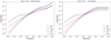 |
Fig. 9 Chemical evolution of P-bearing molecules as a function of time for a diffusion-to-desorption ratio Eb ∕ED of 0.3 (with quantum tunneling) shown in the left panel and for a Eb∕ED of 0.77 (without quantum tunneling) in the right panel. |
Estimated absorption line intensities for the (1–0) transitions of HCP, CP, PN, and PO towards B0355+508 for Tex = 2.73 K, a FWHM linewidth of Δv = 0.5 km s−1 and based on the predicted abundances given by our best-fit model at t = 107 yr.
Acknowledgements
We thank the anonymous referee for his/her comments that significantly improved the present manuscript. The authors also wish to thank the IRAM Granada staff for their help during the observations. V.M.R. has received funding from the European Union’s Horizon 2020 research and innovation programme under the Marie Skłodowska-Curie grant agreement No 66493. Work by A.V. is supported by the Latvian Science Council via the project lzp-2018/1-0170. J.C. acknowledges Dr. J. C. Laas for his support with the Python programming.
Appendix A The depletion of phosphorus
The main advantage of studying the early phases of star formation is to avoid high levels of elemental depletion and thus to constrain the initial abundances used in our model to their cosmic values. This is crucial especially for phosphorus, as the small number of detections of P-bearing species in the ISM makes the determination of the P-depletion level quite difficult. In order to obtain an approximate estimation of the expected depletion level, we apply a dynamical model with time-dependent physical conditions that allows us to follow the chemical evolution of P-bearing species from a diffuse to a dense cloud. In particular we simulate a “cold” stage in which a free-fall collapse takes place within 106 yr (Vasyunin & Herbst 2013; Garrod & Herbst 2006). During that time the density increases from n(H) = 300 to 105 cm−3 and the visual extinction rises from 1 to 40 mag. The gas temperature decreases from 40 to 10 K, while the dust temperature drops slightly, from 20 to 10 K. Finally, the cosmic-ray ionization rate also changes from 1.7 × 10⁻¹⁶ s−1 to 1.3 × 10⁻¹⁷ s−1. We note here that the changes in the above-mentioned physical constants happen within 106 yr, while the total chemical evolution is over 107 yr. This means that between 106 and 107 yr the model becomes static with the above parameters retaining the values they reached at 106 yr. That way, we simulate a long-lived collapse that provides enough time for chemical processes such as depletion to evolve.
As a first step, we plot the chemical evolution of the sum of abundances of gas-phase and solid-phase P-bearing species separately (see lower left panel of Fig. A.1). It is clearly visible how at late times, the gas-phase species decrease, and in return the grain species increase in abundance due to depletion. In particular, the sum of the gas-phase abundances of P-bearing species reduces by a factor of ~ 3000 at t = 107 yr. This does not correspond to the elemental depletion, but it indicates the redistribution of phosphorus between the gas phase and the dust grains. The right-hand panel of Fig. A.1 shows the time-dependent abundances of the main carriers of phosphorus in the gas phase and on grains. The species that experience the largest change during the transition from diffuse to dense cloud are P+ and gPH3. The P+ abundance strongly decreases down to ~10−16, mainly through its destruction reactions with OH, CH4, S, and H2. Atomic P decreases significantly because of freeze-out on dust grains, which is also evident through the increase in gP. According to the model almost all P that freezes out, quickly reacts with hydrogen on grains, and finally forms gPH3 (after successive hydrogenation), which reaches a high abundance of ~2.5 × 10⁻⁷ at the end of our simulations.
Finally, Fig. A.2 shows the time-dependent abundances of PN, PO, HCP, CP, PH3 in the gas phase (left panel) and the corresponding grain species (right panel). All species reach their peak abundances at around 106 yr, followed by a strong decrease due to freeze-out on dust grains as well as through their reaction with  (at t = 106−107 yr). The species PN, PH3, and HCP show a more significant freeze-out than CP and PO, as they are the most abundant molecules in the gas-phase at t = 106 yr. The freeze-out process is also clearly evident from the substantial increase of the corresponding grain species once high densities of ~ 104−105 cm−3 are reached (see right panel of Fig. A.2.)
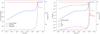 |
Fig. A.1 Results of our dynamical model that simulates the transition from a diffuse to a dense cloud. Left panel: sum of abundances of all P-bearing species in the gas phase (red line) and the solid phase (blue line) as a function of time. Right panel: chemical evolution of the main carriers of phosphorus in the gas and solid phase: P+, P, gP and gPH3. In both figures the density profile of the free-fall collapse is depicted as a black dashed line. |
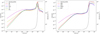 |
Fig. A.2 Chemical evolution of PN, PO, HCP, CP and PH3 (left panel) and the corresponding grain species (right panel) as a function of time based on our dynamical model (diffuse to dense cloud). The black dashed line illustrates the density profile of the free-fall collapse. The gPH3 abundance is shown in Fig. A.1. |
References
- Adams, N. G., McIntosh, B. J., & Smith, D. 1990, A&A, 232, 443 [NASA ADS] [Google Scholar]
- Agudo, I. 2017, in Submm/mm/cm QUESO Workshop 2017 (QUESO2017), 1 [NASA ADS] [Google Scholar]
- Agúndez, M., & Wakelam, V. 2013, Chem. Rev., 113, 8710 [Google Scholar]
- Agúndez, M., Cernicharo, J., & Guélin, M. 2007, ApJ, 662, L91 [NASA ADS] [CrossRef] [Google Scholar]
- Agúndez, M., Cernicharo, J., Decin, L., Encrenaz, P., & Teyssier, D. 2014a, ApJ, 790, L27 [NASA ADS] [CrossRef] [Google Scholar]
- Agúndez, M., Cernicharo, J., & Guélin, M. 2014b, A&A, 570, A45 [NASA ADS] [CrossRef] [EDP Sciences] [Google Scholar]
- Anicich, V. G. 1993, ApJS, 84, 215 [NASA ADS] [CrossRef] [Google Scholar]
- Asplund, M., Grevesse, N., & Jacques Sauval, A. 2006, Nucl. Phys. A, 777, 1 [NASA ADS] [CrossRef] [Google Scholar]
- Bailleux, S., Bogey, M., Demuynck, C., Liu, Y., & Walters, A. 2002, J. Mol. Spectr., 216, 465 [NASA ADS] [CrossRef] [Google Scholar]
- Bizzocchi, L., Esposti, C. D., Dore, L., & Puzzarini, C. 2005, Chem. Phys. Lett., 408, 13 [NASA ADS] [CrossRef] [Google Scholar]
- Caffau, E., Andrievsky, S., Korotin, S., et al. 2016, A&A, 585, A16 [NASA ADS] [CrossRef] [EDP Sciences] [Google Scholar]
- Caselli, P., & Ceccarelli, C. 2012, A&ARv, 20, 56 [NASA ADS] [CrossRef] [MathSciNet] [Google Scholar]
- Cazzoli, G., Puzzarini, C., & Lapinov, A. V. 2004, ApJ, 611, 615 [NASA ADS] [CrossRef] [Google Scholar]
- Cazzoli, G., Cludi, L., & Puzzarini, C. 2006, J. Mol. Struct., 780, 260 [NASA ADS] [CrossRef] [Google Scholar]
- Cecchi-Pestellini, C., Duley, W. W., & Williams, D. A. 2012, ApJ, 755, 119 [NASA ADS] [CrossRef] [Google Scholar]
- Charnley, S. B., & Millar, T. J. 1994, MNRAS, 270, 570 [NASA ADS] [CrossRef] [Google Scholar]
- Chin, Y. N., Henkel, C., Whiteoak, J. B., Langer, N., & Churchwell, E. B. 1996, A&A, 305, 960 [NASA ADS] [Google Scholar]
- Corby, J. F., McGuire, B. A., Herbst, E., & Remijan, A. J. 2018, A&A, 610, A10 [NASA ADS] [CrossRef] [EDP Sciences] [Google Scholar]
- Dalgarno, A. 1988, Astrophys. Lett. Commun., 26, 153 [NASA ADS] [Google Scholar]
- De Beck, E., Kamiński, T., Patel, N. A., et al. 2013, A&A, 558, A132 [NASA ADS] [CrossRef] [EDP Sciences] [Google Scholar]
- Dixon, T. A., & Woods, R. C. 1977, J. Chem. Phys., 67, 3956 [NASA ADS] [CrossRef] [Google Scholar]
- Dupuy, R., Bertin, M., Féraud, G., et al. 2017, A&A, 603, A61 [NASA ADS] [CrossRef] [EDP Sciences] [Google Scholar]
- Fayolle, E. C., Bertin, M., Romanzin, C., et al. 2013, A&A, 556, A122 [NASA ADS] [CrossRef] [EDP Sciences] [Google Scholar]
- Fontani, F., Rivilla, V. M., Caselli, P., Vasyunin, A., & Palau, A. 2016, ApJ, 822, L30 [NASA ADS] [CrossRef] [Google Scholar]
- Fontani, F., Rivilla, V. M., van der Tak, F. F. S., et al. 2019, MNRAS, 489, 4530 [NASA ADS] [CrossRef] [Google Scholar]
- Fuente, A., Navarro, D. G., Caselli, P., et al. 2019, A&A, 624, A105 [NASA ADS] [CrossRef] [EDP Sciences] [Google Scholar]
- Garrod, R. T., & Herbst, E. 2006, A&A, 457, 927 [NASA ADS] [CrossRef] [EDP Sciences] [Google Scholar]
- Godard, B., Falgarone, E., & Pineau des Forêts, G. 2014, A&A, 570, A27 [NASA ADS] [CrossRef] [EDP Sciences] [Google Scholar]
- Gottlieb, C. A., Myers, P. C., & Thaddeus, P. 2003, ApJ, 588, 655 [NASA ADS] [CrossRef] [Google Scholar]
- Hasegawa, T. I., & Herbst, E. 1993, MNRAS, 261, 83 [NASA ADS] [CrossRef] [Google Scholar]
- Hasegawa, T. I., Herbst, E., & Leung, C. M. 1992, ApJS, 82, 167 [NASA ADS] [CrossRef] [Google Scholar]
- Indriolo, N., & McCall, B. J. 2012, ApJ, 745, 91 [NASA ADS] [CrossRef] [Google Scholar]
- Jiménez-Serra, I., Viti, S., Quénard, D., & Holdship, J. 2018, ApJ, 862, 128 [NASA ADS] [CrossRef] [Google Scholar]
- Jura, M., & York, D. G. 1978, ApJ, 219, 861 [NASA ADS] [CrossRef] [Google Scholar]
- Klapper, G., Lewen, F., Gendriesch, R., Belov, S. P., & Winnewisser, G. 2000, J. Mol. Spectr., 201, 124 [NASA ADS] [CrossRef] [Google Scholar]
- Le Petit, F., Roueff, E., & Herbst, E. 2004, A&A, 417, 993 [NASA ADS] [CrossRef] [EDP Sciences] [Google Scholar]
- Lebouteiller, V., Kuassivi, V., & Ferlet, R. 2006, ASP Conf. Ser., 348, 480 [NASA ADS] [Google Scholar]
- Lefloch, B., Vastel, C., Viti, S., et al. 2016, MNRAS, 462, 3937 [NASA ADS] [CrossRef] [Google Scholar]
- Leung, C. M., Herbst, E., & Huebner, W. F. 1984, ApJS, 56, 231 [NASA ADS] [CrossRef] [Google Scholar]
- Liszt, H. S. 2007, A&A, 476, 291 [NASA ADS] [CrossRef] [EDP Sciences] [Google Scholar]
- Liszt, H. S. 2017, ApJ, 835, 138 [NASA ADS] [CrossRef] [Google Scholar]
- Liszt, H. S., & Lucas, R. 1998, A&A, 339, 561 [NASA ADS] [Google Scholar]
- Liszt, H., & Lucas, R. 2001, A&A, 370, 576 [NASA ADS] [CrossRef] [EDP Sciences] [Google Scholar]
- Liszt, H. S., Pety, J., & Lucas, R. 2008, A&A, 486, 493 [NASA ADS] [CrossRef] [EDP Sciences] [Google Scholar]
- Liszt, H., Gerin, M., Beasley, A., & Pety, J. 2018, ApJ, 856, 151 [NASA ADS] [CrossRef] [Google Scholar]
- Lucas, R., & Liszt, H. 1998, A&A, 337, 246 [NASA ADS] [Google Scholar]
- Lucas, R., & Liszt, H. S. 2000, A&A, 358, 1069 [NASA ADS] [Google Scholar]
- Lucas, R., & Liszt, H. S. 2002, A&A, 384, 1054 [NASA ADS] [CrossRef] [EDP Sciences] [Google Scholar]
- Maas, Z. G., Pilachowski, C. A., & Cescutti, G. 2017, ApJ, 841, 108 [NASA ADS] [CrossRef] [Google Scholar]
- McElroy, D., Walsh, C., Markwick, A. J., et al. 2013, A&A, 550, A36 [NASA ADS] [CrossRef] [EDP Sciences] [Google Scholar]
- Millar, T. J. 1991, A&A, 242, 241 [NASA ADS] [Google Scholar]
- Millar, T. J., Bennett, A., & Herbst, E. 1987, MNRAS, 229, 41P [NASA ADS] [CrossRef] [Google Scholar]
- Mininni, C., Fontani, F., Rivilla, V. M., et al. 2018, MNRAS, 476, L39 [NASA ADS] [CrossRef] [Google Scholar]
- Öberg, K. I., Fuchs, G. W., Awad, Z., et al. 2007, ApJ, 662, L23 [NASA ADS] [CrossRef] [Google Scholar]
- Öberg, K. I., Linnartz, H., Visser, R., & van Dishoeck, E. F. 2009, ApJ, 693, 1209 [NASA ADS] [CrossRef] [Google Scholar]
- Pety, J. 2005, in SF2A-2005: Semaine de l’ Astrophysique Francaise, eds. F. Casoli, T. Contini, J. M. Hameury, & L. Pagani (Les Ulis, France: EDP Sciences), 721 [Google Scholar]
- Pety, J., Lucas, R., & Liszt, H. S. 2008, A&A, 489, 217 [NASA ADS] [CrossRef] [EDP Sciences] [Google Scholar]
- Rivilla, V. M., Fontani, F., Beltrán, M. T., et al. 2016, ApJ, 826, 161 [NASA ADS] [CrossRef] [Google Scholar]
- Rivilla, V. M., Jiménez-Serra, I., Zeng, S., et al. 2018, MNRAS, 475, L30 [NASA ADS] [CrossRef] [Google Scholar]
- Ruffle, D. P., & Herbst, E. 2000, MNRAS, 319, 837 [NASA ADS] [CrossRef] [Google Scholar]
- Saito, S., Yamamoto, S., Kawaguchi, K., et al. 1989, ApJ, 341, 1114 [NASA ADS] [CrossRef] [Google Scholar]
- Saykally, R. J., Szanto, P. G., Anderson, T. G., & Woods, R. C. 1976, ApJ, 204, L143 [NASA ADS] [CrossRef] [Google Scholar]
- Schaefer, L., & Fegley, Jr. B. 2011, ApJ, 729, 6 [NASA ADS] [CrossRef] [Google Scholar]
- Snow, T. P., & McCall, B. J. 2006, ARA&A, 44, 367 [NASA ADS] [CrossRef] [Google Scholar]
- Tenenbaum, E. D., Woolf, N. J., & Ziurys, L. M. 2007, ApJ, 666, L29 [NASA ADS] [CrossRef] [Google Scholar]
- Thiel, V., Belloche, A., Menten, K. M., et al. 2019, A&A, 623, A68 [NASA ADS] [CrossRef] [EDP Sciences] [Google Scholar]
- Thorne, L. R., Anicich, V. G., Prasad, S. S., & Huntress, W. T. J. 1984, ApJ, 280, 139 [NASA ADS] [CrossRef] [Google Scholar]
- Turner, B. E., & Bally, J. 1987, ApJ, 321, L75 [NASA ADS] [CrossRef] [Google Scholar]
- Turner, B. E., Tsuji, T., Bally, J., Guelin, M., & Cernicharo, J. 1990, ApJ, 365, 569 [NASA ADS] [CrossRef] [Google Scholar]
- Vasyunin, A. I., & Herbst, E. 2013, ApJ, 762, 86 [NASA ADS] [CrossRef] [Google Scholar]
- Vasyunin, A. I., Caselli, P., Dulieu, F., & Jiménez-Serra, I. 2017, ApJ, 842, 33 [Google Scholar]
- Wakelam, V., Herbst, E., Le Bourlot, J., et al. 2010, A&A, 517, A21 [NASA ADS] [CrossRef] [EDP Sciences] [Google Scholar]
- Wakelam, V., Loison, J.-C., Herbst, E., et al. 2015, ApJS, 217, 20 [NASA ADS] [CrossRef] [Google Scholar]
- Ziurys, L. M., Schmidt, D. R., & Bernal, J. J. 2018, ApJ, 856, 169 [NASA ADS] [CrossRef] [Google Scholar]
We used a Tex of 6 K for deriving N(13CO), as it was inferred in Liszt & Lucas (1998).
All Tables
Derived upper limits for the opacity and the column density of HCP, CP, PN, and PO.
Observed abundances for the cloud component with vLSR = −17 km s−1 and predictions of the species HNC, CO, CS, and CN based on our best-fit model at the time of best agreement t = 6.2 × 10⁶ yr.
Set of physical parameters that give the best agreement between model results and observations towards every cloud component.
Main formation and destruction mechanisms for the species PN, PO, HCP, CP, and PH3 based on the best-fit chemical model at times: t = 103, 105, 107 yr.
Observed and predicted abundances at time t = 107 yr for the species PO, PN, HCP, CP, and PH3 given by our best-fit model.
Predicted abundances of the species PN, PO, HCP, CP, and PH3 at t = 107 yr for three different cosmic-ray ionization rates (see text for explanation).
Predicted abundances of the species PN, PO, HCP, CP, and PH3 as well as H2 at t = 107 yr for three different sets of surface mobility parameters (see text for explanation).
Estimated absorption line intensities for the (1–0) transitions of HCP, CP, PN, and PO towards B0355+508 for Tex = 2.73 K, a FWHM linewidth of Δv = 0.5 km s−1 and based on the predicted abundances given by our best-fit model at t = 107 yr.
All Figures
|
Fig. 1 Spectra of the nondetected (2–1) transitions of PO, PN, HCP, and CP. The upper x-axis shows the rest frequency (in MHz) and the lower one is a velocity axis (in km s−1). The red dashed line indicates the 3σ level and the blue dashed line shows the transition frequency of the corresponding molecule. In the case of PO, we show as an example one of the observed transitions at 108.998 GHz. |
| In the text | |
|
Fig. 2 Spectra of the detected species HNC, CN, C34S, and 13 CO in the 3 mmrange towards the line of sight to the extragalactitc source B0355+508. The red line represents the CLASS Gaussian fit. |
| In the text | |
|
Fig. 3 Detected hyperfine components of the CN (1–0) transition between 113.12 and 113.20 GHz. The three strongest hyperfine components were detected in the three clouds with vLSR =−8, − 10, − 17 km s−1 except for the one weak transition (N, F) = (1, 1∕2) - (0, 1∕2), which was identified only in the two densest clouds (at − 10, − 17 km s−1). |
| In the text | |
|
Fig. 4 Results of the grid of models applying typical conditions for diffuse or translucent clouds in order to reproduce the observations towards the cloud at vLSR =−17 km s−1. The deviation between observations and model at the time of best agreement tbest is given by D(tbest, r), which is plotted versus density, temperature, and visual extinction. The best-fit model is given at a time tbest = 6.2 × 10⁶ yr and has the following parameters: (n(H), AV, Tgas) = (300 cm−3, 3 mag, 40 K). |
| In the text | |
|
Fig. 5 Chemical evolution of the abundances of CO, CN, CS and HNC over 107 yr predicted by our best-fit model with the parameters (n(H), AV, Tgas) = (300 cm−3, 3 mag, 40 K). The colored horizontal bands correspond to the observed abundances towards the cloud with vLSR =−17 km s−1, including the inferred uncertainties. The vertical dashed line indicates the time of best agreement (t = 6.2 × 10⁶ yr) between observations and model results. |
| In the text | |
|
Fig. 6 Variation of the predicted abundances of PN, PO, HCP, CP and PH3 over 107 yr in our best-fit model. The dashed lines represent the 3σ upper limits derived from the observations at vLSR = −17 km s−1. In the case of PO we use 5 × 10⁻¹⁰ as an upper limit (see Table 9 and text for explanation). |
| In the text | |
|
Fig. 7 Predicted abundances of P-bearing molecules as a function of visual extinction AV. The molecular abundances shown here are computed at t = 107 yr. Right panel: predicted abundances of |
| In the text | |
|
Fig. 8 Chemical evolution of P-bearing molecules as a function of time under the effects of cosmic-ray ionization rates of ζ(CR) = 1.7 × 10⁻¹⁶ s−1 (left panel) and 10.6 × 10⁻¹⁶ s−1 (right panel). |
| In the text | |
|
Fig. 9 Chemical evolution of P-bearing molecules as a function of time for a diffusion-to-desorption ratio Eb ∕ED of 0.3 (with quantum tunneling) shown in the left panel and for a Eb∕ED of 0.77 (without quantum tunneling) in the right panel. |
| In the text | |
|
Fig. A.1 Results of our dynamical model that simulates the transition from a diffuse to a dense cloud. Left panel: sum of abundances of all P-bearing species in the gas phase (red line) and the solid phase (blue line) as a function of time. Right panel: chemical evolution of the main carriers of phosphorus in the gas and solid phase: P+, P, gP and gPH3. In both figures the density profile of the free-fall collapse is depicted as a black dashed line. |
| In the text | |
|
Fig. A.2 Chemical evolution of PN, PO, HCP, CP and PH3 (left panel) and the corresponding grain species (right panel) as a function of time based on our dynamical model (diffuse to dense cloud). The black dashed line illustrates the density profile of the free-fall collapse. The gPH3 abundance is shown in Fig. A.1. |
| In the text | |
Current usage metrics show cumulative count of Article Views (full-text article views including HTML views, PDF and ePub downloads, according to the available data) and Abstracts Views on Vision4Press platform.
Data correspond to usage on the plateform after 2015. The current usage metrics is available 48-96 hours after online publication and is updated daily on week days.
Initial download of the metrics may take a while.