VIS3COS

Ana Paulino-Afonso; David Sobral; Behnam Darvish; Bruno Ribeiro; Ian Smail; Philip Best; Andra Stroe; Joseph Cairns

doi:10.1051/0004-6361/201834244

Home

All issues

Volume 633 (January 2020)

A&A, 633 (2020) A70

Full HTML

Free Access

Issue		A&A Volume 633, January 2020


Article Number		A70
Number of page(s)		19
Section		Extragalactic astronomy
DOI		https://doi.org/10.1051/0004-6361/201834244
Published online		14 January 2020

A&A 633, A70 (2020)

VIS³COS

III. Environmental effects on the star formation histories of galaxies at z ∼ 0.8 seen in [O II], Hδ, and D_n4000^⋆^⋆⋆

Ana Paulino-Afonso¹^,2^,3, David Sobral³, Behnam Darvish⁴, Bruno Ribeiro⁵, Ian Smail⁶, Philip Best⁷, Andra Stroe⁸ and Joseph Cairns³

¹ Instituto de Astrofísica e Ciências do Espaço, Universidade de Lisboa, OAL, Tapada da Ajuda, 1349-018 Lisboa, Portugal
e-mail: aafonso@oal.ul.pt, asofiafonso@gmail.com
² Departamento de Física, Faculdade de Ciências, Universidade de Lisboa, Edifício C8, Campo Grande, 1749-016 Lisboa, Portugal
³ Department of Physics, Lancaster University, Lancaster LA1 4YB, UK
⁴ Cahill Center for Astrophysics, California Institute of Technology, 1216 East California Boulevard, Passadena, CA 91125, USA
⁵ Leiden Observatory, Leiden University, PO Box 9513, 2300 RA Leiden, The Netherlands
⁶ Centre for Extragalactic Astrophysics, Department of Physics, Durham University, Durham DH1 3LE, UK
⁷ Institute for Astronomy, University of Edinburgh, Royal Observatory, Blackford Hill, Edinburgh EH9 3HJ, UK
⁸ Harvard-Smithsonian Center for Astrophysics, 60 Garden Street, Cambridge, MA 02138, USA

Received: 14 September 2018
Accepted: 8 November 2019

Abstract

We present spectroscopic observations of 466 galaxies in and around a superstructure at z ∼ 0.84 targeted by the VIMOS Spectroscopic Survey of a Supercluster in the COSMOS field (VIS³COS). We use [OII]λ3727, Hδ, and D_n4000 to trace recent, medium-, and long-term star formation histories and investigate the effect of stellar mass and local environment on them. By studying trends in individual and composite galaxy spectra, we find that stellar mass and environment play a role in the observed galactic properties. Galaxies with low stellar mass (10 < log₁₀(M_⋆/M_⊙) < 10.5) in the field show the strongest Hδ absorption. Similarly, the massive population (log₁₀(M_⋆/M_⊙) > 11) shows an increase in Hδ absorption strengths in intermediate-density environments (e.g. filaments). Galaxies with intermediate stellar mass (10.5 < log₁₀(M_⋆/M_⊙) < 11) have similar Hδ absorption profiles in all environments, but show an indication of enhanced [OII] emission in intermediate-density environments. This indicates that field galaxies with low stellar mass and filament galaxies with high stellar mass are more likely to have experienced a recent burst of star formation, while galaxies of the intermediate stellar-mass show an increase of star formation at filament-like densities. We also find that the median [OII] equivalent width (|EW_[OII]|) decreases from 27 ± 2 Å to 2.0^+0.5_−0.4 Å and D_n4000 increases from 1.09 ± 0.01 to 1.56 ± 0.03 with increasing stellar mass (from ∼10^9.25 to ∼10^11.35 M_⊙). For the dependence on the environment, we find that at fixed stellar mass, |EW_[OII]| is tentatively lower in environments with higher density. We find for D_n4000 that the increase with stellar mass is sharper in denser environments, which indicates that these environments may accelerate galaxy evolution. Moreover, we find higher D_n4000 values in denser environments at fixed stellar mass, suggesting that galaxies are on average older and/or more metal rich in these dense environments. This set of tracers depicts a scenario where the most massive galaxies have, on average, the lowest specific star formation rates and the oldest stellar populations (age ≳ 1 Gyr, showing a mass-downsizing effect). We also hypothesize that the observed increase in star formation (higher EW_[OII]|, higher specific star formation rate) at intermediate densities may lead to quenching because we find that the quenched fraction increases sharply from the filament to cluster-like regions at similar stellar masses.

Key words: galaxies: evolution / galaxies: high-redshift / galaxies: star formation / large-scale structure of Universe

^⋆

A copy of the reduced spectra is available at the CDS via anonymous ftp to cdsarc.u-strasbg.fr (130.79.128.5) or via http://cdsarc.u-strasbg.fr/viz-bin/cat/J/A+A/633/A70

^⋆⋆

Based on observations obtained with VIMOS on the ESO/VLT under the programmes 086.A-0895, 088.A-0550, and 090.A-0401.

© ESO 2020

1. Introduction

One of the key tracers of galactic evolution is the rate at which gas is converted into stars. This is measured as the star formation rate (SFR, e.g. Kennicutt 1998; Kennicutt & Evans 2012). Observations show that typical galaxies were actively forming stars at a rate that was ∼10 times higher at z ∼ 2 than at z ∼ 0 (both the cosmic SFR density and typical SFRs decrease during this epoch, see e.g. Madau & Dickinson 2014; Sobral et al. 2014). One of the fundamental questions of modern Astronomy is to understand the mechanisms that are responsible for the regulation of star formation in galaxies and find how efficient galaxies are in converting gas into stars (see e.g. Combes et al. 2013; Lehnert et al. 2013).

Two broad groups of processes, internal and external, can contribute to the evolution of any given galaxy (e.g. Kormendy 2013). However, the contribution of each set of processes to regulating star formation in galaxies is still unclear (see e.g. Erfanianfar et al. 2016). Internal processes include dynamical instabilities (e.g. Kormendy 2013), halo quenching (e.g. Birnboim & Dekel 2003; Kereš et al. 2005, 2009b; Dekel & Cox 2006), supernova feedback (e.g. Efstathiou 2000; Cox et al. 2006), and active galactic nuclei (AGN) feedback (e.g. Bower et al. 2006; Croton et al. 2006; Somerville et al. 2008; Fabian 2012). External processes include galaxy interactions with other galaxies or the intergalactic medium, specifically, ram pressure stripping (e.g. Gunn & Gott 1972), galaxy strangulation (e.g. Larson et al. 1980; Balogh et al. 2000), galaxy-galaxy interactions and harassment (e.g. Mihos & Hernquist 1996; Moore et al. 1998), or tidal interaction between the large-scale gravitational potential and the galaxy (e.g. Merritt 1984; Fujita 1998). These ranges of physical processes are thought of as the way through which galaxies are regulated, and they eventually halt the formation of new stars. This phenomenon is commonly referred to as galaxy quenching (e.g. Gabor et al. 2010; Peng et al. 2010a).

The way in which each proposed mechanism affects individual galaxies is complex. In internal processes, feedback can either heat or eject the gas from galaxies, preventing it from condensing in molecular clouds to form new stars (e.g. Kereš et al. 2009a). Supernova feedback is thought to be more important at lower stellar masses, and AGN feedback is arguably an important mechanism for quenching at high stellar masses (e.g. Puchwein & Springel 2013). Halo quenching refers to gravitational heating, preventing gas from cooling and forming new stars. However, it requires a sustained mechanism to heat the gas (e.g. Birnboim et al. 2007), and cold gas flows might still penetrate the halo into the galactic disc to fuel star formation (e.g. Kereš et al. 2009b).

In terms of external processes, ram pressure stripping can initially compress the gas or dust, thus increasing the column density of the gas and dust, which is favourable for star formation (e.g. Gallazzi et al. 2009a; Bekki 2009; Owers et al. 2012; Roediger et al. 2014). Tidal galaxy-galaxy interactions can lead to the compression and inflow of the gas in the periphery of galaxies into the central parts, feeding and rejuvenating the stellar populations in the central galactic regions, which results in an enhancement in star formation activity (e.g. Mihos & Hernquist 1996; Kewley et al. 2006; Ellison et al. 2008). Such encounters are probable when the galaxies have low relative velocities (i.e. low-velocity dispersion environments) and are closer to each other (denser regions). Intermediate-density environments such as galaxy groups, in-falling regions of clusters, cluster outskirts, merging clusters, and galaxy filaments provide the ideal conditions for such interactions (e.g. Moss 2006; Perez et al. 2009; Li et al. 2009; Sobral et al. 2011; Tonnesen & Cen 2012; Darvish et al. 2014; Stroe et al. 2014, 2015; Malavasi et al. 2017). This enhancement of star formation is thought to be responsible for the subsequent quenching because most of the available gas is consumed or expelled through outflows in a short period of time, effectively preventing future star formation from occurring in the galaxy without further external influence. If those events are ubiquitous, a temporary rise in star formation in such environments should be observed, after which galaxies are expected to become passive. This has been found in several studies, which referred to the intermediate-density environments as sites of enhanced SFR and obscured star formation activity (e.g. Smail et al. 1999; Best 2004; Koyama et al. 2008, 2010, 2013; Gallazzi et al. 2009a; Geach et al. 2009; Sobral et al. 2011, 2016; Coppin et al. 2012; Stroe et al. 2015, 2017).

Because many of these mechanisms are linked to the increased density of galaxies, it is natural to search over-dense regions for the effect of the local environment on the observed properties of galaxy populations. In the local Universe (z ∼ 0), star formation is typically lower in higher density environments (e.g. Oemler 1974; Dressler 1980; Lewis et al. 2002; Kauffmann et al. 2004; Blanton et al. 2005; Li et al. 2006; Peng et al. 2010a; Darvish et al. 2016, 2018). By separating galaxies into distinct populations (star-forming and quiescent), studies found that the quenched fraction is highly dependent on the local density, at least up to z ≲ 1, with the quenched population being more common in high-density regions and a higher fraction of star-forming galaxies found in lower density regions (e.g. Kodama et al. 2001, 2004; Best 2004; Nantais et al. 2013; Darvish et al. 2016; Erfanianfar et al. 2016; Cohen et al. 2017). While the picture is clear in the local Universe, with the average star formation being the lowest in high-density relaxed cluster regions (e.g. Balogh et al. 2000; Kauffmann et al. 2004), it is still unclear if it holds at higher redshifts. Some studies found a flattening and/or reversal of this relation (z ∼ 1 − 1.5, e.g. Cucciati et al. 2006; Elbaz et al. 2007; Ideue et al. 2009; Tran et al. 2010; Popesso et al. 2011; Li et al. 2011; Santos et al. 2014; Stach et al. 2017; Cooke et al. 2019), while others found the same trends we see locally (e.g. Patel et al. 2009; Sobral et al. 2011; Muzzin et al. 2012; Santos et al. 2013; Scoville et al. 2013; Darvish et al. 2016). It is possible that reconciling the different observed trends requires more detailed analyses of other possible underlying relations, especially with stellar mass (e.g. Peng et al. 2010a; Sobral et al. 2011; Muzzin et al. 2012; Darvish et al. 2016), and also controlling for other properties such as AGN fraction and dust content. An alternative explanation might be the stochastic nature of the formation of dense environments, which can explain the observed differences as a natural cosmic variance.

Recent studies have used the spectral indices [OII], Hδ, and D_n4000 to probe the stellar population of galaxies at intermediate redshifts (0.5 ≲ z ≲ 1.2) because they are available in the observed optical frame. All these indicators, when combined, can be used to distinguish actively star-forming, (post-) starburst, and old or passive galaxies because they are expected to occupy different regions of the possible parameter space (e.g. Couch & Sharples 1987; Balogh et al. 1999; Poggianti et al. 1999, 2009; Fritz et al. 2014). The [OII]λ3737 emission traces on-going star formation (timescales of ∼10 Myr, e.g. Couch & Sharples 1987; Poggianti et al. 1999, 2006; Kennicutt 1998; Kewley et al. 2004), but it also depends on the metallicity and can be a poor tracer for dusty galaxies (e.g. Kewley et al. 2004; Yan et al. 2006; Kocevski et al. 2011). By measuring the [OII] equivalent width (EW), we can also crudely trace the specific SFR (sSFR), which is found to be anti-correlated with stellar mass (e.g. Bridge et al. 2015; Cava et al. 2015; Darvish et al. 2015a), with more massive star-forming galaxies having lower [OII] EWs. Additionally, higher density environments are found to depress [OII] emission (e.g. Balogh et al. 1999; Darvish et al. 2015a). The H_δ line (and other strong Balmer absorption lines) can be indicative of a post-starburst phase (≈100 − 1000 Myr after the burst, e.g. Couch & Sharples 1987; Balogh et al. 1999; Poggianti et al. 1999, 2009; Dressler et al. 2004; Vergani et al. 2010; Mansheim et al. 2017a) if a strong absorption (typical of A stars, where hydrogen absorption is strongest) is observed and no tracers of on-going star formation are found (Couch & Sharples 1987). Recently, Wu et al. (2018) found that the Hδ EW correlates with stellar mass, with more massive galaxies having weaker Hδ absorption lines, but they did not study the effect of the environment (see also e.g. Siudek et al. 2017, for a similar result on passive galaxies). Finally, a measure of the flux break at 4000 Å (D4000 and D_n4000, as defined by Bruzual 1983; Balogh et al. 1999, respectively) traces the age of the galaxy and also the stellar metallicity (especially for older systems) to a lesser degree. This break is produced by a combination of metal absorption on the atmosphere of old and cool stars and the lack of flux from young and hot OB stars (e.g. Poggianti & Barbaro 1997; Kauffmann et al. 2003), and so it is sensitive to the average age of the stellar population. The 4000 Å break is also found to be stronger for galaxies with higher stellar mass (e.g. Muzzin et al. 2012; Vergani et al. 2008; Hernán-Caballero et al. 2013; Siudek et al. 2017; Wu et al. 2018), which indicates that their stellar populations might be older, in an average sense. In terms of local density, Muzzin et al. (2012) found that galaxies in cluster environments have stronger breaks on average than their field counterparts at similar stellar masses, which the authors argued can be explained by the different fractions of star-forming and quiescent galaxies in different environments.

We aim to investigate the influence of the environment on the star formation history of galaxies using a number of spectral indicators (e.g. Balogh et al. 1999; Poggianti et al. 1999, 2009; Dressler et al. 2004; Vergani et al. 2010; Mansheim et al. 2017b; Wu et al. 2018). Based on the spectral coverage of the VIMOS Spectroscopic Survey of a Superstructure in the COSMOS field (VIS³COS, Paulino-Afonso et al. 2018, hereafter PA18), we estimate the current and past star formation activity of galaxies using a combination of [OII] (tracing on-going star formation in moderately to highly star-forming galaxies, ≲10 Myr), Hδ (probing star formation on intermediate timescales – 50 Myr to ∼1 Gyr prior to observation), and D_n4000 (probing the star formation history on longer timescales). We investigate this using spectroscopic observations of ∼500 galaxies in and around a superstructure at z ∼ 0.84 in the COSMOS field (Sobral et al. 2011, PA18) by probing a wide range of environments and stellar masses with a single survey.

This paper is organized as follows: in Sect. 2 we briefly explain the survey and give some details on the data we used. Section 3 details the stacking methods and the spectroscopic measurements. In Sect. 4 we present the results from individual and stacked spectral properties. We discuss our findings in Sect. 5. Section 6 presents the conclusions of our study. We use AB magnitudes (Oke & Gunn 1983), a Chabrier (Chabrier 2003) initial mass function (IMF), and assume a ΛCDM cosmology with H₀ = 70 km s⁻¹ Mpc⁻¹, Ω_M = 0.3, and Ω_Λ = 0.7. The physical scale at the redshift of the superstructure (z ∼ 0.84) is 7.63 kpc/″.

2. VIS³COS survey

2.1. Survey description

The VIS³COS survey maps a large z ∼ 0.84 over-density spanning 21′ × 31′ (9.6 × 14.1 Mpc²) in the COSMOS field (Scoville et al. 2007) with the VIMOS instrument mounted on the Very Large Telescope (VLT). This structure contains three confirmed X-ray clusters (Finoguenov et al. 2007) and also harbours a large-scale over-density of Hα emitters (Sobral et al. 2011; Darvish et al. 2014). The full description of the data and redshift measurements are presented in PA18, and we briefly describe some details here.

Our primary targets were selected from the Ilbert et al. (2009) catalogue and with 0.8 < z_phot, l < 0.9 (with z_phot, l being either the upper or lower 99% confidence interval limit for each source) and i_AB < 22.5. To effectively fill the masks, we also added as secondary targets galaxies down to i_AB < 23 with photometric redshifts in the interval 0.6 < z < 1.1. For the selected targets we obtained high-resolution spectra with the VIMOS High-Resolution red grism (with the GG475 filter, R ∼ 2500). This grism covers the 3400 − 4600 Å rest-frame at the redshift of the target superstructure. The observational configuration of the survey was done so that we could measure spectral features such as [O II] λ3726,λ3729 (partially resolved doublet), the 4000 Å break, and Hδ for the superstructure members. We have compared our spectroscopic sample with a mass-complete catalogue and corrected for sample incompleteness following the procedure detailed in Sect. 2.2.

We measured the redshifts of our sources using SPECPRO (Masters & Capak 2011) on the extracted 1D spectra and using a combination of [OII], H+K absorption, G band, some Fe lines, and Hδ. All spectra were visually inspected for the features described above. We obtained secure spectroscopic redshifts for 696 sources with high signal-to-noise ratio (S/N), of which 490 are at 0.8 < z < 0.9. Spectroscopic failures are related to either low S/N continuum or the lack of apparent features.

With the knowledge of the spectroscopic redshift, we improved the estimate of physical parameters that are available in the COSMOS2015 photometric catalogue (Laigle et al. 2016). We ran MAGPHYS (da Cunha et al. 2008) with spectral models constructed from the stellar libraries by Bruzual & Charlot (2003) and using photometric bands from near-UV to near-IR. The dust was modelled following the prescription described by Charlot & Fall (2000). We obtained estimates for the stellar masses and SFRs for 466 out of the 490 galaxies that were observed at 0.8 < z < 0.9. Galaxies with no estimates are mostly fainter i-band secondary sources with no match in COSMOS2015 or are not included in the latter catalogue due to different selection bands. Comparing our spectroscopic redshifts with the photometric redshifts of the COSMOS2015 catalogue, we find a dispersion σ_{Δz/(1 + z)} = 0.009. The scatter in stellar mass and SFR for galaxies with |z_spec − z_phot|< 0.1 is ∼0.15 dex and ∼0.6 dex, respectively. For this study, we used SFRs derived with the spectral energy distribution (SED) because the observed [OII] emission is a poor tracer of SFR for red, low SFR galaxies (with non-detections in quiescent sources) and depends on gas-phase metallicity (e.g. Kewley et al. 2004; Yan et al. 2006; Kocevski et al. 2011), and we have no independent way to quantify dust extinction or measure metallicity from our spectral coverage. We note that problems and limitations inevitably affect SED-derived SFRs (especially when young stellar populations dominate galaxies, see e.g. Wuyts et al. 2011), but they mostly affect high SFR galaxies (> 50 M_⊙ yr⁻¹), which is a small portion (< 13%) of our sample. We refer to PA18 for a comparison between SED- and [OII]-derived SFRs for our sample.

Our final sample was restricted to be at 0.8 < z < 0.9 to match our primary selection (see PA18) and had a total of 466 galaxies spanning a wide range of environments across several Mpc. We show in Fig. 1 the colour-magnitude diagram (r − z versus z-band, corresponding roughly to rest-frame U − V versus V) and the stellar mass-SFR relation from our sample and compare it to the parent photometric catalogue. We note that our sample becomes close to a sample that is complete in stellar mass at stellar masses greater than 10¹⁰ M_⊙.

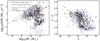Fig. 1.

Stellar masses and SFRs derived from SED fitting in our spectroscopic sample at 0.8 < z < 0.9, showing the primary (filled circles) and secondary (open circles) targets separately (left). Colour-magnitude diagram for the same sample (right). For comparison, we show the derived best-fit relation for star-forming galaxies computed at z = 0.84 using the equation derived by Whitaker et al. (2012) over a large average volume in the COSMOS field (the dashed line is an extrapolation below their stellar mass completeness). The vertical dotted line shows the approximate stellar-mass representativeness limit of our survey. The dotted contours show the COSMOS2015 distribution of galaxies with 0.8 < z_phot < 0.9 and i_AB < 22.5 from 10% to 90% of the sample in 10% steps.

To estimate the local galaxy over-density, we used the density fields computed by Darvish et al. (2015b, 2017). These results are based on the photometric redshift catalogue in the COSMOS field provided by Ilbert et al. (2013). The density field was calculated for a ∼1.8 deg² area using a mass-limited (log₁₀(M/M_⊙) > 9.6) sample at 0.1 < z_phot < 1.2. In this paper we define as over-density

$\begin{matrix} 1 + δ = \frac{Σ}{Σ_{median}}, \end{matrix}$ $\begin{aligned} 1+\delta = \frac{\Sigma }{\Sigma _\mathrm{median} }, \end{aligned}$ (1)

with Σ_median being the median of the density field of a specific redshift slice. We used an adaptive kernel with variable size, with small kernel size for crowded regions and larger kernel size for sparser regions, around a typical width of 0.5 Mpc (characteristic size of X-ray clusters, see e.g. Finoguenov et al. 2007). We note that re-computing the density field using the spectroscopic redshifts from our sample does not significantly change the underlying density fields. For a more detailed description of the method, we refer to Darvish et al. (2015b, 2017). A pure density-based definition of the environment does not translate exactly into different physical regions (see e.g. Aragón-Calvo et al. 2010; Darvish et al. 2014). In each density bin we can have a mix of different regions, that is, dense filamentary structures can have local densities similar to that of the core of rich galaxy groups or cluster outskirts, and small groups could share the same local density as scarcely populated filaments. Nonetheless, there are typical densities at which field (log₁₀(1 + δ)≲0.1), filament (0.1 ≲ log₁₀(1 + δ)≲0.6), and cluster galaxies (log₁₀(1 + δ)≳0.6) dominate the population (see PA18 for more details).

2.2. Completeness corrections

The nature of spectroscopic surveys means that it is hard to observe all galaxies in a field down to a single magnitude or stellar mass limit. To ensure that our final spectroscopic sample is as representative as possible of the global population over the same field, we used the excellent wealth of data available in the COSMOS field to quantify the representativeness of our sample. Specifically, we used the COSMOS2015 catalogue, which is reported to be mass complete down to 10^9.4 M_⊙ for quiescent galaxies at these redshifts (mass-completeness limit is 10⁹ M_⊙ when all galaxies in the observed region are considered; Laigle et al. 2016). In Fig. 2 we show the relative fraction of galaxies in our spectroscopic sample compared to the mass-complete sample from the COSMOS2015 catalogue. When the samples are split into the star-forming and quiescent populations, we find different incompleteness effects. Our completeness for quiescent galaxies starts to drop at stellar masses below 10^10.5 M_⊙, and we fail to detect a single quiescent galaxy in the lower stellar mass bin (10⁹ M_⊙ − 10^9.5 M_⊙). For star-forming galaxies our completeness drops at lower stellar masses (below 10^9.5 M_⊙).

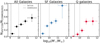Fig. 2.

Number of galaxies with spectroscopic redshifts in VIS³COS divided by the number of galaxies in the mass-complete COSMOS2015 catalogue over the same region and limited to 0.8 < z_phot < 0.9 for all, star-forming, and quiescent galaxies. The vertical dashed lines correspond to the mass-complete limits in COSMOS2015. The vertical dotted lines correspond to our quoted limiting mass of ∼10¹⁰ M_⊙. The error bars are computed from Poisson statistics.

We assigned weights to all of our galaxies in our sample based on the position of the stellar mass, specific SFR, and local over-density with respect to the mass-complete population at 0.8 < z_phot < 0.9. In practice, we computed the fraction of galaxies that is observed in the three-dimensional region centred on each target in the mass-complete catalogue and compared this to the fraction of galaxies in our spectroscopic sample in the same region,

$\begin{matrix} w_{i} = \frac{N_{mass, R_{i}}}{N_{spec, R_{i}}} \times \frac{N_{spec}}{N_{mass}}, \end{matrix}$ $\begin{aligned} { w}_i = \frac{N_{\mathrm{mass} ,R_i}}{N_{\mathrm{spec} ,R_i}} \times \frac{N_\mathrm{spec} }{N_\mathrm{mass} }, \end{aligned}$ (2)

where N_mass represents the numbers of galaxies in the complete mass catalogue, N_spec is the number of galaxies in the spectroscopic catalogue, and the index R_i means that the variable is computed inside the region that surrounds galaxy i. To define each region, we used a ellipsoidal selection on the three-dimensional space with a size of 0.25 in the log₁₀(M_⋆/M_⊙) dimension, 1 in the log₁₀(sSFR) dimension, and 0.5 in the log₁₀(1 + δ) dimension.

We expect that these corrections are valid for all galaxies above 10⁹ M_⊙, which is the quoted mass-completeness limit for star-forming galaxies at these redshifts (Laigle et al. 2016). However, because our primary selection would translate into a limiting mass (considering all galaxies) of approximately 10¹⁰ M_⊙ (this is the median stellar mass of all 22.3 < i_AB < 22.7 and 0.8 < z_phot < 0.9 galaxies in the COSMOS2015 catalogue) and this is reflected in the low completeness values at these stellar masses (see Fig. 2), we restricted our analysis to galaxies above this stellar-mass threshold. For the sub-populations of star-forming galaxies, our primary i-band selection translates into different limiting stellar masses. For the star-forming population, our i-band selection would typically select galaxies down to 10^9.9 M_⊙. For the quiescent population, the same selection would be limited at 10^10.6 M_⊙. We tried to account for this effect by weighting galaxies based on their position in the stellar mass−sSFR plane, which aims to minimize this selection bias.

3. Spectroscopic properties

3.1. Composite spectra

Co-adding spectra of galaxies that were binned by similar physical properties increases the S/N and allows a better determination of the median spectral properties of the sample in different regions of the parameter space that we aim to probe (e.g. Lemaux et al. 2010). We constructed composite spectra by binning in stellar mass, over-density, and SFR. For a quick view on the different composite spectra, see Figs. A.1–A.3.

To obtain composite spectra, we first normalized each spectrum to the mean flux measured in the range 4150−4350 Å. Using the redshift we measured (see Sect. 2), we linearly interpolated the spectrum onto a common universal grid (3250 − 4500 Å, Δλ = 0.5 Å pix⁻¹). We then computed the median flux at each wavelength in the grid to obtain the final composite spectra. We normalized each spectrum by dividing it by the median flux measured at 4150 − 4350 Å. We assigned a weight to each spectrum based on the completeness corrections detailed in Sect. 2.2. Finally, we obtained the composite spectra as the weighted median flux per wavelength bin in the defined grid. We repeated our analysis using different normalization schemes (blueward of 4000 Å and with no normalization), and our results were qualitatively the same.

3.2. Spectral quantities

To study the star formation history of galaxies, we used three tracers: [OII], Hδ, and D_n4000 that are present in our spectra (e.g. Balogh et al. 1999; Dressler et al. 2004; Oemler et al. 2009; Poggianti et al. 2009; Vergani et al. 2010; Mansheim et al. 2017a). To be consistent with the classical notation, a negative EW corresponds to a line in emission, and positive values correspond to a line in absorption.

3.2.1. [OII] emission

To measure the [OII], we fit a double Gaussian to the doublet. The centre of each component was set to be λ₁ = 3726.08 ± 0.3 Å and λ₂ = 3728.88 ± 0.3 Å (a small shift in the line centre was allowed to account for our finite resolution, and we allowed for a systematic shift to the doublet to account for redshift uncertainties). We measured the flux and line EWs by integrating over the best-fit models. For more details we refer to PA18 (see also Fig. 3, left panel).

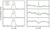Fig. 3.

Three examples of the fit to the stacked [O II] emission (left) and the stacked Hδ absorption + emission (right) spectral lines. The solid black line shows the observed spectrum. The green line shows the median fit (after 10 000 realizations), and the orange line is the estimated continuum around the line. We also show in red and blue dashed lines the fit of each Gaussian component.

3.2.2. Hδ in emission and absorption

We fit the emission and absorption components of the Hδ line using a double-Gaussian fit with two independent components (see Fig. 3, right panel): one forced to have a negative amplitude (for the absorption), and the other forced to have a positive amplitude (for the emission). To prevent a set of degenerate model combinations that produce the same combined result, but for which the individual components are clearly not physically representative of the observed data¹, we forced the width of the emission line to be always smaller than the absorption component. This is informed by the empirical information from the individual stacks we obtained. To estimate the first-guess amplitude of the absorption, we took the minimum of the continuum subtracted spectra. The amplitude of the emission line was computed by first fitting a single Gaussian to the absorption feature (whenever present), masking the ±3 Å around the central wavelength, and then taking the maximum of the absorption subtracted spectra. We also assigned an initial σ of 4 and 1 Å for the absorption and emission component. We then measured the line fluxes and EWs from the best-fit models.

3.2.3. Continuum and error estimation

For all line fits we individually defined two regions (one blue-ward and one red-ward of the line) with a width of 15 Å width (about three times the spectral resolution) from which we estimated the median continuum level. Then the local continuum was defined as a straight line through these two points (see e.g. Balogh et al. 1999; Lemaux et al. 2010; Mansheim et al. 2017a). To minimize the effect of a particular choice of windows from which we computed the continuum, we computed the median flux for 5000 random shifts of kÅ on the proposed interval, where k was randomly drawn from a normal distribution centred at 0 and with a width of 5 Å. Then the final estimate of the continuum was measured from the median of the 5000 realizations.

To estimate the errors on the derived spectral quantities, we performed a bootstrap sampling of each sub-sample of spectra. This method allowed us to estimate the variance that occurs within each sub-sample. This quoted error is always larger than the formal uncertainties from the fit. We performed the fit on 1000 individual bootstrapped spectra (using only 80% random galaxies drawn from the sub-sample) and derived the final errors from the 16th and 84th percentiles of the distribution of best-fit values.

3.2.4. 4000 Å break

In addition to line measurements, we also computed the strength of the break at 4000 Å (D4000; D_n4000 defined by Bruzual 1983; Balogh et al. 1999, respectively). We automated the computation of these quantities by integrating the spectra over the red (D4000: 4050−4250 Å, D_n4000: 4000−4100 Å) and blue (D4000: 3750−3950 Å, D_n4000: 3850−3950 Å) intervals and computing the ratio of these fluxes as

$\begin{matrix} X 4000 = \frac{\int_{λ_{r 1}}^{λ_{r 2}} f_{ν} d λ}{\int_{λ_{b 1}}^{λ_{b 2}} f_{ν} d λ}, \end{matrix}$ $\begin{aligned} X4000 = \frac{\int _{\lambda _{r1}}^{\lambda _{r2}} f_\nu \mathrm{d}\lambda }{\int _{\lambda _{b1}}^{\lambda _{b2}} f_\nu \mathrm{d}\lambda }, \end{aligned}$ (3)

where X is either D or D_n, depending on the integration limits of the red (λ_ri) and blue (λ_bi) intervals. When we compare these two indices, we find them to correlate well, with a median difference of < 1% and a spread of 30% on individual measurements. We opted to use the value of D_n4000 for the remainder of the paper because it is expected to be less affected by errors from Poisson sampling and less affected by reddening (Balogh et al. 1999). Nevertheless, our results are qualitatively the same, regardless of which index we used. To avoid contamination by emission lines in the integrated regions, we masked 6 Å regions around the [NeIII] and Hζ lines (see e.g. Fig. A.1).

3.3. Stellar population age estimates

Estimating a single representative stellar age for galaxies is not a trivial task because their star formation histories are expected to vary. Nonetheless, we can obtain an estimate given a few sets of assumptions. We used the D_n4000 index as a proxy for age and obtained an estimate from a set of stellar population models described by Bruzual & Charlot (2003). We attempted to estimate an age based on a single stellar population (SSP), with the notation t_SSP, which should trace the age of the last major burst that the galaxy had.

We note that the D_n4000 index depends not only on age, but also on the stellar metallicity, especially for ages greater than 1 Gyr (e.g. Bruzual 1983; Poggianti & Barbaro 1997; Balogh et al. 1999). We do not have any independent way to estimate stellar metallicity for all galaxies, therefore we need to make a few assumptions to try and mitigate possible bias in our interpretations. We assumed that our sample follows the stellar mass-metallicity relation that is found locally and up to z ∼ 1 (e.g. Tremonti et al. 2004; Gallazzi et al. 2005; Savaglio et al. 2005; Zahid et al. 2011, 2013; Ma et al. 2016; De Rossi et al. 2017; Leethochawalit et al. 2018). We then estimated individual stellar metallicities based on a recent numerical simulation study by Ma et al. (2016), which parametrizes stellar metallicity as a function of stellar mass and redshift as

$\begin{matrix} {log}_{10} (\frac{Z_{⋆}}{Z_{⊙}}) = 0.40 [{log}_{10} (\frac{M_{⋆}}{M_{⊙}}) - 10] + 0.67 e^{- 0.5 z} - 1.04 . \end{matrix}$ $\begin{aligned} \log _{10}\left(\frac{Z_\star }{{Z}_\odot }\right) = 0.40\left[\log _{10}\left(\frac{M_\star }{{M}_\odot }\right) - 10\right] +0.67e^{-0.5z}-1.04. \end{aligned}$ (4)

For a stellar mass (10^10.5 M_⊙) and for the redshift (z = 0.84) of our sample, we determine a stellar metallicity of Z_⋆ ∼ 0.008 = Z_⊙/2.5. For a stellar mass of 10^11.5 M_⊙, we obtain Z_⋆ ∼ 0.02, and for a stellar mass 10^9.5 M_⊙, we obtain Z_⋆ ∼ 0.003. We show the age dependence of D_n4000 for different stellar metallicities that span the expected range of our sample in Fig. 4.

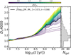Fig. 4.

Value of D_n4000 as a function of stellar age for a set of single stellar population models from Bruzual & Charlot (2003) for different stellar metallicities from Z = 0.1 Z_⊙ to Z = 2.5 Z_⊙. The thick solid line shows the relation using the stellar metallicity for the median stellar mass and redshift of our sample (see Sect. 3.3). Right panel: distribution of measured D_n4000 values for the galaxies in our sample.

To estimate the age of a galaxy (or group of galaxies), we first computed the individual (or median) stellar metallicity and then used the D_n4000-age relation for an SSP based on Bruzual & Charlot (2003) models at that metallicity to derive the stellar age. The errors on the SSP ages were derived as detailed in Sect. 3.2.3 and do not include any uncertainty on the metallicity.

4. Results

We explored the results on the spectral properties of our galaxies at 0.8 < z < 0.9, highlighting both composite spectra and individual galaxies in this section. We aimed to probe the influence of key physical properties (stellar mass, environment, and SFR) on the median observed spectral properties of our sample. We note that for Hδ the S/N on most galaxies is insufficient for robust measurements, and we refrain from discussing this spectral feature in terms of individual galaxies.

We summarize in Fig. 5 (see also Appendix A and Table A.1) the properties of composite spectra on [OII] and Hδ (both emission and absorption) line EWs and D_n4000 at different stellar masses, over-densities, and SFRs. We stress that for samples that were not selected in stellar mass, we imposed a minimum stellar mass limit of 10¹⁰ M_⊙.

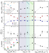Fig. 5.

Dependence of the three spectral features detailed in Sect. 3.2 (from top to bottom: [OII] EW, Hδ EWs, and D_n4000) as a function of stellar mass (left), over-density (middle), and SED-derived SFR (right). We show our stellar mass representativeness limit as a vertical dotted line in the left panels and show as empty symbols the measurements for which the completeness effects are large. We note that for bins that are not defined in stellar mass (middle and right panels), the composite spectra are built from galaxies with stellar mass greater than 10¹⁰ M_⊙. Results from this paper are shown as large symbols connected by a dotted line with associated error bars derived from the 16th and 84th percentiles of the 1000 bootstrapped fits (when the error bars are not shown, it implies an error smaller than the symbol size). The trends with stellar mass show a decrease in [OII] and Hδ emission (blue squares) and absorption (red circles) strength and an increase in the average age of the stellar population (traced by D_n4000). The trends with over-density show a peak in [OII] EW at filament-like densities, and Hδ EWs show little dependence on local density. There is also a clear trend that galaxies are older in higher density regions. Lastly, the strength of [OII] and Hδ increases with SFR (except for the most strongly star-forming galaxies), and younger populations lie in galaxies with higher SFR, as expected. We compare our results to other surveys in the literature (Bridge et al. 2015; Darvish et al. 2015a; Cava et al. 2015; Wu et al. 2018; Hernán-Caballero et al. 2013; Vergani et al. 2008; Muzzin et al. 2012). For a more detailed discussion of the differences, we refer to Sects. 4.2.1 and 4.2.2.

4.1. Global trends on the spectroscopic properties

4.1.1. Stellar mass

We discuss here the trends of the measured spectroscopic properties as a function of the stellar mass. While we show in Fig. 5 the results at stellar masses between 10⁹ M_⊙ and 10¹⁰ M_⊙, we do not discuss them because this results suffer from high incompleteness (see Sect. 2.2).

In terms of the [OII] line EW (EW_[OII]), we find in Fig. 5 a strong decrease with stellar mass, by a factor of ∼3 in strength from the lowest (10 < log₁₀(M_⋆/M_⊙) < 10.5) to the highest stellar mass bin (log₁₀(M_⋆/M_⊙) > 11), which points to a decrease in sSFR with increasing stellar mass from ∼10⁻⁹ yr⁻¹ to ∼10⁻¹⁰ yr⁻¹ (a consequence of the main sequence of star-forming galaxies, see also Darvish et al. 2015a). We compare the results for individual galaxies and composite spectra with others available in the literature (Bridge et al. 2015; Cava et al. 2015; Darvish et al. 2015a). Our results are broadly consistent (in terms of the observed trends) with the literature, which finds a decrease in the absolute line EW with increasing stellar mass. However, we find some discrepancies with Cava et al. (2015) and Bridge et al. (2015) in terms of the average value in bins of stellar mass that are likely related to the target selection in each work. Cava et al. (2015) reported consistently higher values of [OII] line EW. However, their sources were selected through medium-band filters down to EWs of ∼15−20 Å, which naturally explains their higher median values. Bridge et al. (2015) studied a large field with blind spectroscopy and excluded galaxies with large EWs (EW ≳ 40 Å) to avoid contamination by interlopers with higher redshift (Lyα emitters), which can explain their observed lower EWs. We find EW_[OII] values consistent with Darvish et al. (2015a), whose observational setup was similar to that of the VIS³COS survey.

In the middle panels of Fig. 5 we show the measured EW of the Hδ emission and absorption for all composite spectra that allowed a measurement (some of them did not show any signs of absorption). The Hδ absorption line EW decreases with increasing stellar mass (from EW_Hδ = 2.7 ± 0.2 Å at 10 < log₁₀(M_⋆/M_⊙) < 10.5 down to EW $_{H δ} = 1 . 1_{- 0.2}^{+ 0.3}$ $_{\mathrm{H\delta}} = 1.1_{-0.2}^{+0.3}$ Å at log₁₀(M_⋆/M_⊙) > 11). The Hδ emission line EW also correlates with stellar mass: stronger emission is found at lower stellar masses, dropping from EW $_{H δ} = - 0 . 6_{- 0.2}^{0.3}$ $_{\mathrm{H\delta}} = -0.6_{-0.2}^{0.3}$ Å at 10 < log₁₀(M_⋆/M_⊙) < 10.5 to a marginally non-existent emission component with EW_Hδ = −0.1 ± 0.1 Å at log₁₀(M_⋆/M_⊙) > 11. When we compare this to the results by Wu et al. (2018), we see that their reported EW also decreases with stellar mass but at a steeper rate. We attribute the discrepancies to the different methods that were used to compute the line EW. They used a spectral index defined by Worthey & Ottaviani (1997), which measures the line EW on an emission subtracted or masked spectrum. We also show the dependence of the emission-to-absorption ratio of the EWs as a proxy for the ratio of O to A stars. Our results are consistent with no dependence on stellar mass.

The bottom panels of Fig. 5 show the dependence of the 4000 Å break strength on the same quantities as above. We find a strong correlation between D_n4000 and stellar mass, increasing from $D_{n} 4000 = 1 . 27_{- 0.01}^{+ 0.02}$ $D_n4000=1.27_{-0.01}^{+0.02}$ at 10 < log₁₀(M_⋆/M_⊙) < 10.5 to D_n4000 = 1.56 ± 0.03 at log₁₀(M_⋆/M_⊙) > 11. This trend indicates that more massive galaxies also have older stellar populations. Our results are in general agreement with other studies in the literature that targeted either clustered regions (VVDS, SHARDS, and LEGA-C, see Vergani et al. 2008; Hernán-Caballero et al. 2013; Wu et al. 2018, respectively). The trend with stellar mass is seen in all surveys. We find median values in between the quoted average or median of other studies in the literature at similar redshifts. We find lower median D_n4000 at fixed stellar masses with respect to values reported by Muzzin et al. (2012) for cluster galaxies, which is expected given the dependence of D_n4000 seen with the environment and the fact that we probed a majority population at lower densities than the cluster sample. This is consistent with what we find when the sample is split into stellar mass and local density bins, with galaxies at fixed stellar mass having the stronger 4000 Å breaks at the higher densities we probe (see Sect. 4.2).

4.1.2. Local environment

Our analysis is restricted to stellar masses greater than 10¹⁰ M_⊙, and for this sub-sample, the median stellar mass varies little across the different bins (Δlog₁₀(M_⋆/M_⊙) < 0.15). We find that the absolute value of EW_[OII] increases from $4 . 0_{- 0.6}^{+ 0.5}$ $4.0^{+0.5}_{-0.6}$ Å to $6 . 5_{- 0.5}^{+ 0.4}$ $6.5^{+0.4}_{-0.5}$ Å from field to filament-like densities and then drops to $2 . 7_{- 0.3}^{+ 0.5}$ $2.7^{+0.5}_{-0.3}$ Å in our highest density bin. This indicates a slight increase in the sSFR at filament-like densities for galaxies that are more massive than 10¹⁰ M_⊙ and then a strong drop towards the higher density regions probed here. We also compared the trends with local density to those with environmental regions (field, filament, and cluster, see Table A.1), as defined in PA18 (see also Darvish et al. 2015b, 2017) and find a decline of $| EW [O I I] |$ $|\mathrm{EW}[{\mathrm{O}\,\textsc{ii}}]|$ from field to filament to cluster regions (from $4 . 6_{- 0.4}^{+ 0.5}$ $4.6^{+0.5}_{-0.4}$ Å to $4 . 4_{- 0.4}^{+ 0.3}$ $4.4^{+0.3}_{-0.4}$ Å to 3.4 ± 0.5 Å, respectively) for galaxies more massive than 10¹⁰ M_⊙. These differences reflect the nuances of using different tracers of the galactic environment, but both reinforce a drop of EW[OII] towards the denser regions studied here.

For the Hδ absorption line, we find results that are consistent with no trend with local density. For Hδ emission, all our derived values for galaxies more massive than 10¹⁰ M_⊙ are also consistent with no dependence with over-density; the measured EWs are around ∼0−0.5 Å. We find no significant dependence on over-density on the results regarding the ratio between absorption and emission of Hδ, given our error bars.

Finally, we find an increase of D_n4000 towards higher densities. In low- to intermediate-density regions (log₁₀(1 + δ) < 0.5), we find D_n4000 ∼ 1.26 − 1.31 (corresponding to an SSP age of ∼0.35 − 0.47 Gyr). The strength of the 4000 Å break then increases at higher densities (log₁₀(1 + δ) > 0.5), reaching D_n4000 = 1.51 ± 0.02 (corresponding to an SSP age of ∼1.1 ± 0.1 Gyr).

4.1.3. Star formation rate

Our analysis is restricted to stellar masses greater than 10¹⁰ M_⊙, which probes a range of 3 dex in SFR. We note that the difference in the median or mean stellar mass in each defined SFR bins is smaller than 0.1 dex, which means that the correlations of the studied tracers with SFR are not affected by an underlying SFR-stellar mass relation. This is so because at stellar masses > 10¹⁰ M_⊙ the spread in SFRs is strong because star-forming and quiescent galaxies of similar stellar mass exist at these masses.

Overall, the EW[OII] increases with increasing SFR. We find a strong increase from the quiescent (low-SFR) population (−1.4 ± 0.2 Å for log₁₀(SFR) < 0.4) to the active (intermediate-SFR) star-forming population (∼−7.5 Å) in our sample. Then we find a small increase towards the high-SFR population (−10.3 ± 0.5 Å for log₁₀(SFR) > 1.2).

For the Hδ absorption component, we find a small increase of the EW with SFR, from EW_Hδ ≈ 1.9 − 1.4 ± 0.25 Å at log₁₀(SFR [M_⊙ yr⁻¹]) < 0.8 to EW_Hδ ≈ 2.4 − 2.6 ± 0.25 Å at log₁₀(SFR [M_⊙ yr⁻¹]) > 0.8. The correlation of the Hδ emission with SFR mirrors what we find with [O II] emission: the line strength increases from low to high SFRs (from $- 0 . 1_{- 0.3}^{+ 0.1}$ $-0.1_{-0.3}^{+0.1}$ Å to −0.8 ± 0.1 Å). The emission to absorption line ratio is marginally consistent with no trend with SFR (though we see a rise on the median value from low to intermediate-high SFR galaxies).

Finally, we observe a steady decrease in the value of D_n4000 from the lowest SFR bin (D_n4000 = 1.47 ± 0.01 for log₁₀(SFR [M_⊙ yr⁻¹]) < 0.4) to the highest SFR bin (D_n4000 = 1.19 ± 0.01 for log₁₀(SFR [M_⊙ yr⁻¹]) > 1.2). This is consistent with what is expected from the evolution of galaxies because we expect a larger fraction of young stars in highly star-forming galaxies. This decreases the value of D_n4000.

4.2. Distinguishing environment and stellar mass effects

To distinguish the effects of stellar mass and environment, we explored our sample binned into stellar mass and over-density bins. We chose the over-density bins in a way that they were representative of field (low-density), filament (intermediate-density), and cluster outskirts (high-density) regions (see PA18 for more details). We show the influence of the over-density in the observed spectroscopic properties in three different bins of stellar mass (chosen as a compromise for a reasonable S/N for Hδ) for individual galaxies and composite spectra.

4.2.1. EW_[OII]

We show in Fig. 6 the relation between [OII] line EW and stellar mass for individual galaxies with an [OII] detection, which should mainly trace star-forming galaxies, although we find a ∼10% contamination (17 out of 166 [OII] emitters) in our > 10¹⁰ M_⊙ sample from low sSFR (log₁₀(sSFR) < − 11) galaxies (see also e.g. Yan et al. 2006; Lemaux et al. 2010). We attempted to separate the effects of local density on this correlation and found that the correlation between [OII] line EW and stellar mass is similar in all environments. We found similar gradients at all environments and fit a linear relation with a fixed slope (the average of individually fitted slopes)² for all environments:

$\begin{matrix} {EW}_{[OII]} = 8.05 \times {log}_{10} (M_{⋆} / 10^{10} M_{⊙}) + b . \end{matrix}$ $\begin{aligned} \mathrm{EW} _\mathrm{[OII]} = 8.05\times \log _{10}\left(M_\star /10^{10}\,{M_\odot }\right) + b. \end{aligned}$ (5)

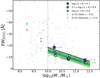Fig. 6.

Relation between [OII] EW and stellar mass for the [OII]-emitters in our sample in three different over-density bins. We compare our results (large green and dark blue symbols are the median of the population, and the same smaller symbols represent individual measurements) with results from Darvish et al. (2015a) of filament and field galaxies, as small red and blue triangles, respectively. We show the best fit (with error estimate) from Eq. (5) for each density bin as shaded regions. We show that higher stellar mass galaxies have weaker [OII] emission, and this relation is seen in all over-density subsets.

The best-fit values are shown in Table 1. Line EWs should be insensitive to dust if continuum and line flux are emitted from the same regions. We note, however, that the attenuation of stellar and nebular emission in the local Universe is different (e.g. Calzetti et al. 2000; Wild et al. 2011), and it seems to be less pronounced at higher redshifts (z ≳ 1, e.g. Kashino et al. 2013; Pannella et al. 2015). We tentatively find a lower [OII] EW with increasing density, but all relations are within 1σ uncertainties. This is consistent with no dependence of the sSFR on environment for a star-forming population (e.g. Muzzin et al. 2012; Koyama et al. 2013; Darvish et al. 2016, PA18).

Table 1.

Results of the linear fits X = m × log₁₀(M_⋆/10¹⁰ M_⊙)+b to EW_[OII] and D_n4000 that are shown in Figs. 6 and 7.

Concerning the results from composite spectra, we show in Fig. 8 an overall trend [O II] line EW with stellar mass (as reported in Fig. 6) at each over-density bin. We show that [OII] depends on the stellar mass and on the environment of galaxies. For galaxies with lower stellar mass (10 < log₁₀(M_⋆/M_⊙) < 10.5), we find a small decrease in EW_[OII] with increasing local density. Intermediate-mass galaxies (10.5 < log₁₀(M_⋆/M_⊙) < 11) show a small rise (at the 1.7σ level) in EW_[OII] from field to filament-like regions and then a small decrease towards cluster-like regions. The most massive galaxies are consistent with no environmental effect on the [OII] emission. The local density dependence of the EW[OII] emission in the stacked spectra can be reconciled with the apparent environmentally independent estimates we show in Fig. 6. We include in the stacking analysis all the galaxies with no [OII] emission (either quiescent or dusty), which are known to be more common in higher density regions (quiescent: e.g. Peng et al. 2010a; Cucciati et al. 2010; Sobral et al. 2011; Muzzin et al. 2012; Darvish et al. 2016; PA18; dusty star formation: e.g. Smail et al. 1999; Gallazzi et al. 2009b; Koyama et al. 2013; Sobral et al. 2016).

4.2.2. 4000 Å break

The 4000 Å break is a proxy for the age of the underlying stellar population (see Sect. 3.3). Under this assumption, we find that at higher masses (log₁₀(M_⋆/M_⊙) > 10), galaxies residing in high-density regions are typically older than their counterparts in lower density regions. We find that D_n4000 is 5 ± 3% (lower stellar mass, ∼0.3 Gyr difference) to 23 ± 6% (higher stellar mass, ∼2 Gyr difference) higher in high-density regions than in lower density regions, see Fig. 7. There is also an underlying correlation between stellar mass and D_n4000: more massive galaxies have stronger flux breaks at 4000 Å and are therefore older (rising from ∼1.1 to ∼1.35 − 1.65 from lower to higher stellar masses, see also e.g. Vergani et al. 2008; Muzzin et al. 2012; Hernán-Caballero et al. 2013; Wu et al. 2018).

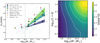Fig. 7.

D_n4000 as a function of stellar mass for three different over-density bins. The vertical dotted line shows the representativeness limit of our survey. We show the best fit (with errors) from Eq. (6) for each density bin as shaded regions. We find an underlying correlation between stellar masses and D_n4000: the median D_n4000 of galaxies in high-density regions is higher than in low-density regions. The difference between low- and high-density environments is larger at higher stellar masses. We compare with the results from GCLASS (Muzzin et al. 2012), from VVDS (Vergani et al. 2008), from SHARDS (Hernán-Caballero et al. 2013), and from LEGA-C (Wu et al. 2018), which also show the same trends. We also show here the median value of D_n4000 as a function of both stellar mass and local density in in the right panel. This map is a smooth interpolation of the trends found in our sample and highlights the increase of the median D_n4000 with increasing stellar mass and local density.

The relative difference between field and cluster galaxies shown by Muzzin et al. (2012) indicates a stronger break in higher density regions, although in their sample, the difference between cluster and field galaxies becomes smaller with increasing stellar mass. This can be interpreted as a stronger dependence of the quenched fraction on environment for lower stellar masses (e.g. Peng et al. 2010a), which is less evident at z ∼ 1 (Muzzin et al. 2012; Darvish et al. 2016; although we do find a dependence for our sample, see PA18). However, the different timescales of the tracer that is used to defined quiescence (we use the SED-based sSFR, which traces the past ∼100 Myr) and D_n4000 also needs to be accounted for, which traces the average age of the stellar population (and can range from several hundreds of megayears to several gigayears; see e.g. Sect. 4.3, where we show that quiescent galaxies in high-density environments have higher D_n4000 than the quiescent population in low-density regions).

We also note that the separation between field and cluster galaxies in Muzzin et al. (2012) was made using the cluster-centric radius (defined as the distance to the brightest cluster galaxy of each of their clusters). Their field sample is representative of a population of galaxies that are in-falling into the clusters, and their cluster galaxies are drawn from a sample of rich clusters. This means that a direct comparison is not straightforward. Thus we find that their field galaxies should correspond to filament-like densities as defined in our paper, and cluster galaxies likely correspond to higher densities than what we probe with the VIS³COS survey. Nonetheless, the quiescent fraction that is reported in Muzzin et al. (2012) is in line with that found in studies where field samples are independent of cluster regions and do not reach rich cluster density regions (van der Burg et al. 2013; Peng et al. 2010a). It is therefore not clear that the definition of field and cluster samples can explain the observed differences in the differential trend of D_n4000 and stellar mass for field and cluster galaxies.

We quantified the increase rate of D_n4000 with the linear model (we fixed the y-intercept to the average of individual fits)³

$\begin{matrix} D_{n} 4000 = m \times {log}_{10} (M_{⋆} / 10^{10} M_{⊙}) + 1.15, \end{matrix}$ $\begin{aligned} D_n4000 = m\times \log _{10}\left(M_\star /10^{10}\,{M_\odot }\right) + 1.15, \end{aligned}$ (6)

where the best-fit values are summarized in Table 1.

We confirm the trend reported on individual galaxies more clearly based on D_n4000 in the composite spectra (see Fig. 8). At fixed density, D_n4000 increases from low to high stellar masses. At fixed stellar mass, D_n4000 increases from low to high-density environments (with the exception at the highest densities, where galaxies between 10¹⁰ M_⊙ and 10¹¹ M_⊙ have similar values of D_n4000). We also find that the difference between different stellar mass bins is different for different density regions. The relation becomes steeper at intermediate densities when compared to the low-density regions probed here. At the higher densities we probe, the difference between the low and intermediate stellar mass bins is smaller, but we find a larger difference towards the highest stellar masses. This indicates that stellar mass and environment both have an effect on the stellar populations of galaxies: higher density environments harbour older galaxies at all stellar masses.

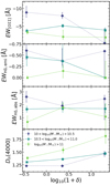Fig. 8.

Dependence of the three spectral indices detailed in Sect. 3.2 (from top to bottom: [OII] EW, Hδ EW, and D_n4000) as a function of over-density in three stellar mass bins. This highlights the impact of stellar mass and environment on the observed spectral properties of galaxies.

4.2.3. Hδ emission and absorption

We also find a dependence on the stellar mass of the strength of the Hδ emission: galaxies with lower stellar mass on average have higher EWs (see Fig. 8, Table A.1). Within our estimated errors, we cannot pinpoint any dependence of the line strength on the environment. Concerning the absorption component of Hδ, the results indicate a dependence on the environment that itself depends on the stellar mass we consider. However, only the rise from low to intermediate densities in absorption EW for higher stellar masses is of some significance (from $0 . 7_{- 0.7}^{+ 0.5}$ $0.7^{+0.5}_{-0.7}$ Å to $1 . 8_{- 0.2}^{+ 0.3}$ $1.8^{+0.3}_{-0.2}$ Å). Interestingly, at intermediate densities, the Hδ absorption line has a similar EW at all stellar masses.

With respect to the emission component of Hδ, we find a tentative trend that the emission is stronger for less massive galaxies (as reported for the full sample in Fig. 5). We find no significant dependence on local density for each of the stellar mass ranges we considered.

4.2.4. Anti-correlation between D_n4000 and EW_[OII]

We show in Fig. 9 an anti-correlation between the strength of the 4000 Å break (traced by D_n4000) and the [OII] line EW. This broadly traces the sSFR (Darvish et al. 2015a). The observed trend seems to be partially induced by a variation in stellar mass, and we find that the most massive galaxies (log₁₀(M_⋆/M_⊙) > 11) in intermediate- and high-density regions show an increase in D_n4000 but have similar [OII] line EWs as lower density regions. We attempt to qualify the correlation by fitting two linear models in two different stellar mass regimes,

$\begin{matrix} Y = {\begin{matrix} (- 3.9 \pm 0.7) \times X + (5.8 \pm 0.9) & if 10 < M < 11 \\ (- 0.8 \pm 0.2) \times X + (1.9 \pm 0.3) & if M > 11 \end{matrix}, \end{matrix}$ $\begin{aligned} Y = {\left\{ \begin{array}{ll} (-3.9\pm 0.7) \times X + (5.8\pm 0.9)&\mathrm{if} \;10 < M < 11\\ (-0.8\pm 0.2) \times X + (1.9\pm 0.3)&\mathrm{if} \;M>11 \end{array}\right.}, \end{aligned}$ (7)

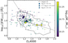Fig. 9.

Observed relation between D_n4000 and log₁₀(−EW_[OII]) for individual galaxies (small symbols) and median per stellar mass bin (large symbols), colour-coded by their stellar mass. The small purple dots show the values for galaxies with log₁₀(M_⋆/M_⊙) < 10. Different symbols correspond to different over-densities. The dashed lines are linear fits to the data of individual galaxies in two stellar mass sub-samples (see text for details): the steeper slope is the fit for galaxies with 10 < log₁₀(M_⋆/M_⊙) < 11, and the shallower slope is the fit for galaxies with log₁₀(M_⋆/M_⊙) > 11. This highlights the underlying anti-correlation between the observed strength of the [OII] emission and the strength of the 4000 Å break. We show as a black contour the location of 85% of the zCOSMOS sample at 0.48 < z < 1.2 with stellar masses greater than 10¹⁰ M_⊙ (Vergani et al. 2010).

with Y = log₁₀(−EW_[OII]), X = D_n4000, and M = log₁₀(M_⋆/M_⊙). This means a steeper slope for the less massive galaxies than the slope for the most massive galaxies. We find that the departure from the lower stellar mass relation occurs at lower stellar masses for higher density regions. Galaxies in field-like regions never depart from this relation.

This relation is qualitatively similar to what is reported for galaxies that are more massive than 10¹⁰ M_⊙ in zCOSMOS at 0.48 < z < 1.2 by Vergani et al. (2010), although they only use this relation to compare the selection of star-forming, quiescent, and post-starburst galaxies. We interpret this relation as a combination of two phenomena. At lower stellar masses (< 10¹¹ M_⊙), it is likely a consequence of a declining sSFR with the stellar mass that drives the decrease of [OII] EW and an increase of D_n4000. At higher stellar masses, other ionizing mechanisms than star formation alone are possible. We note that the fraction of quiescent galaxies is higher at high stellar masses and also higher in the high-density regions we probe; see PA18. It is also found in the literature that for these red systems, the [OII] line is likely dominated by AGN- or low-ionization nuclear emission line (LINER)-powered emission (e.g. Yan et al. 2006; Lemaux et al. 2010). More recently, resolved studies of galaxies have also revealed that LINER-like emission can be widespread and is thought to be powered by an extended population of post-asymptotic red giant branch stars (see e.g. Singh et al. 2013; Gomes et al. 2016; Belfiore et al. 2016, 2017). It is also possible that an increased stellar metallicity would result in an increase of D_n4000 at fixed EW[OII], but there is little evidence that metallicity strongly depends on environment (e.g. for gas-phase metallicity, see Ellison et al. 2009; Cooper et al. 2008; Darvish et al. 2015a; Sobral et al. 2015, 2016; Wu et al. 2017, and for stellar metallicity, see Harrison et al. 2011). Another likely explanation is that there is an underlying older stellar population in higher density environments (as hinted from Sect. 4.2.2) with residual star formation producing the observed [O II] emission. This could be seen through a similar break in the sSFR-D_n4000 relation, which we do not observe as prominently in our sample. However, we cannot test the possible LINER-like emission nature of [OII] without spectroscopic observations at longer wavelengths.

4.3. Star formation activity in different environments

Finally, we also studied the composite spectra of quiescent and star-forming galaxies (more massive than 10¹⁰ M_⊙ separated at SED-derived log₁₀(sSFR) = − 11, see PA18) in low- (log₁₀(1 + δ) < 0.1) and high- (log₁₀(1 + δ) > 0.4) density environments and summarize our results in Fig. 10 (see also Table A.1). We find that the two populations are separated by D_n4000 and EW_[OII], as expected. Overall, we also find that the difference is larger in high-density regions.

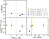Fig. 10.

Properties of composite spectra of quiescent and star-forming galaxies selected according to their sSFR (separation at log₁₀(sSFR) = − 11, see also PA18) in low- (diamonds) and high-density regions (squares). The dotted lines are for D_n4000 = 1.325 and EW_[OII] = 4 Å and are shown to guide the eye. These two populations are separated in D_n4000 and EW_[OII], and some environmental effects can also be found within each population of galaxies. Quiescent and star-forming populations are more clearly separated in high-density regions.

When we focus on the Hδ absorption strength, we see stronger absorption in star-forming galaxies in high-density regions than at lower densities. These results indicate that star-forming galaxies in high-density regions have undergone a recent burst of star formation (or that they are a mix of normal star-forming galaxies with a post-starburst population), or that they have dustier star-forming regions (e.g. Smail et al. 1999). This scenario would explain similar observed [OII] EWs, but a ∼50 ± 20% increase in the Hδ absorption strength and only a small ∼3 ± 2% increase in D_n4000 (see e.g. Balogh et al. 1999; Poggianti et al. 1999; Mansheim et al. 2017a). For field star-forming galaxies we find lower EWs for the Hδ absorption. This may indicate a less bursty star-formation in these systems.

From estimates using a single stellar population model with a stellar mass-based stellar metallicity (see Sect. 3.3), we find that quenched galaxies in the densest regions are much older (assuming an SSP, $\sim 2 . 2_{- 0.4}^{+ 0.1}$ ${\sim}2.2_{-0.4}^{+0.1}$ Gyr) than those in the field ( $\sim 0 . 54_{- 0.07}^{+ 0.09}$ ${\sim}0.54_{-0.07}^{+0.09}$ Gyr). These differences among quiescent galaxies depending on the environment are not found by Muzzin et al. (2012) or Mosleh et al. (2018). We note that the quiescent samples in low- and high-density regions have similar stellar mass distributions, therefore we should not expect this to be a simple consequence of an underlying mass-metallicity relation. We discuss further interpretations of our results in Sect. 5.2.

5. Discussion

Our results highlight that both stellar mass and environment play a role in the star formation history of galaxies. (as also reported by e.g. Iovino et al. 2010; Cucciati et al. 2010; Peng et al. 2010a; Li et al. 2011; Davidzon et al. 2016; Darvish et al. 2016; Kawinwanichakij et al. 2017). Figure 8 shows that the stellar mass influences the strength of the [OII] in all environments, showing weaker emission for the most massive galaxies, and that stellar mass is the main driver of the observed changes. However, we see that the difference between populations of different stellar masses is affected by the environment. A similar result is also seen in Hδ absorption, with field-like regions being the place where most differences are found. This is also clearly visible in D_n4000, where the difference among galaxies with different stellar masses depends on the local density; galaxies in the field are the most similar.

5.1. Environmental effects on star formation

Figure 8 shows that galaxies with stellar masses 10.5 < log₁₀(M_⋆/M_⊙) < 11 show a small increase (at ∼1.7σ level) in the observed emission strength of [OII] at filament-like densities when compared to field and cluster regions (see also Fig. 5 for stacks with all galaxies more massive than 10¹⁰ M_⊙). Although this trend indicates a slightly higher sSFR at intermediate densities, it is not evidence enough of any environmental effect on SFR at these stellar masses.

Considering the sample at 10.0 < log₁₀(M_⋆/M_⊙) < 10.5, we find an overall decrease in the EW[OII] with increasing density, which is also seen for similar stellar masses in Tomczak et al. (2019). At the high stellar mass end of our sample, we see no effect of the environment on the observed EW[OII]. This overall effect on the median sSFR can be linked to the results on the quenched fraction (f_Q) shown in PA18, where we find that at high stellar masses (> 10¹¹ M_⊙) there is no dependence effect on f_Q, while at lower stellar masses there is an increase from intermediate- to high-density regions (see also e.g. Lemaux et al. 2019). An increase of the quenched fraction (from ∼10% to ∼50% of the sample from low- and intermediate- to high-density regions, see Table A.1) results in a lower median sSFR value for the population. These two results point to an environmental dependence of star formation at 10.0 < log₁₀(M_⋆/M_⊙) < 10.5 (see also e.g. Peng et al. 2010b), while for more massive galaxies we see no major effect. This would support a scenario in which mass-quenching mechanisms act to suppress star formation at high stellar masses, and local environment has a negligible impact on star formation (e.g. Peng et al. 2010b, 2012), but more recent studies see a different picture for massive galaxies in dense environments (e.g. Darvish et al. 2016).

A scenario that can explain these results must account for enhancement of star formation activity at intermediate densities and then some quenching mechanism that acts as galaxies move towards higher densities (which may be connected). This can be thought of as filaments being regions of higher probabilities for gas-rich galaxies to interact (e.g. Moss 2006; Perez et al. 2009; Li et al. 2009; Tonnesen & Cen 2012; Darvish et al. 2014; Malavasi et al. 2017), promoting compression of gas clouds and a peak in the SFR of the galaxy (e.g. Mihos & Hernquist 1996; Kewley et al. 2006; Ellison et al. 2008; Gallazzi et al. 2009a; Bekki 2009; Owers et al. 2012; Roediger et al. 2014). We study a superstructure that is composed of several sub-clusters, therefore it is also possible that activity related to cluster-cluster interactions is capable of enhancing star formation as well (e.g. Stroe et al. 2014, 2015; Sobral et al. 2015), although this might not always be the case (see e.g. Mansheim et al. 2017b).

5.2. Older population prevalence influenced by the environment

While we find in Fig. 5 that D_n4000 is strongly correlated with stellar mass, we show in Fig. 8 that the strength of this correlation is strongly dependent on the environment. The fact that cluster galaxies have on average stronger 4000 Å breaks has previously been reported in other studies (see e.g. Muzzin et al. 2012), but we extend it to a range of densities that is complementary to the sample of Muzzin et al. (2012), targeting rich clusters and the galaxies around them.

To explain the observed trend, the time that has passed since the last relevant episode of star formation needs to be different in each environment (see also e.g. Rettura et al. 2010, 2011; Darvish et al. 2016). The most massive galaxies (log₁₀(M_⋆/M_⊙) > 11) have older stellar populations in high-density regions than the lower density region counterparts ( $5_{- 2}^{+ 3}$ $5_{-2}^{+3}$ Gyr compared to $0 . 64_{- 0.07}^{+ 0.06}$ $0.64_{-0.07}^{+0.06}$ Gyr at lower densities⁴). PA18 showed that at these stellar masses, the quenched fraction does not change with the environment, so that it is not simply a larger fraction of red galaxies that can reproduce the age differences. This would then require that massive galaxies in the high-density regions have become passive earlier than their field counterparts. This might mean that denser regions have collapsed first and thus galaxies in these regions formed at earlier times (e.g. Thomas et al. 2005; Nelan et al. 2005). It is also consistent with the observed age difference for quenched galaxies in the field and cluster-like densities ( $\sim 0 . 54_{- 0.07}^{+ 0.09}$ ${\sim}0.54_{-0.07}^{+0.09}$ Gyr and $\sim 2 . 2_{- 0.4}^{+ 0.1}$ ${\sim}2.2_{-0.4}^{+0.1}$ Gyr, respectively).

The lack of recent star formation in higher density regions might be linked to the lower gas accretion in dense regions (e.g. van de Voort et al. 2017). The prevalence of gas stripping in dense regions (e.g. Bahé et al. 2013; Jaffé et al. 2015; Poggianti et al. 2016), which is also seen in the lack of gas-rich galaxies in clusters (e.g. Boselli et al. 2016), means that there is little fuel for new star-forming episodes for massive galaxies. In lower density environments (fields, filaments, or groups), it is more likely that gas can be funnelled to the massive galaxies from minor mergers or tidal interactions with gas-rich satellites (Poggianti et al. 2016). This is also consistent with the pre-processing of galaxies in filaments and groups (gas loss and quiescence) before infall in the cluster regions (Wetzel et al. 2013; Haines et al. 2015). The ram pressure from the denser regions can also act as an enhancement of star formation prior to quenching (see Sect. 5.1 and e.g. Poggianti et al. 2016). Thus, massive galaxies in high-density regions are expected to grow through mergers of gas-poor galaxies (dry mergers, see e.g. Khochfar & Burkert 2003; Khochfar & Silk 2009; McIntosh et al. 2008; Lin et al. 2010; Davidzon et al. 2016; Martin et al. 2017) in order to build up their mass while maintaining an older stellar population. In this scenario, the dependence of the D_n4000 stellar mass on the environment is explained by the fraction of gas-rich galaxies that are available for merging at each density; there are fewer such galaxies at higher densities (e.g. Boselli et al. 2016). This is also in agreement with numerous reported trends of the quenched fraction (equivalent to the number of gas-poor galaxies) with environment (Peng et al. 2010a; Cucciati et al. 2010; Sobral et al. 2011; Muzzin et al. 2012; Darvish et al. 2016; PA18).

At stellar masses 10 < log₁₀(M_⋆/M_⊙) < 11, the effect of environment is less pronounced (differences in D_n4000 between low- and high-density environments are smaller), although we still see slightly older stellar populations in higher density environments (∼0.6 Gyr older than in low-density environments). In this case, we would require either that galaxies are still forming new stars or that if they are quenched, it occurred more recently. Because we observe a rise of the quenched fraction with local density for these stellar masses in PA18, we favour the latter scenario.

We can reconcile the environmental effects seen at high stellar masses in D_n4000 with those seen only at lower stellar masses in EW[OII] and f_Q discussed in Sect. 5.1. The values of EW[OII] and f_Q (directly related to the galaxy sSFR by our definition) probe star formation timescales of 10−100 Myr (e.g. Couch & Sharples 1987; Salim et al. 2007; da Cunha et al. 2008), and the value for D_n4000 can probe the lack of recent star formation on longer timescales (typically a few gigayears, see Sect. 3.3). These different tracers can then be thought of as the difference between a galaxy being quenched or not (instantaneous star formation traced by [OII]) and the time that has passed since that quenching (traced by D_n4000). A simple explanation is possibly linked to the formation epoch of massive galaxies in different environments (e.g. Thomas et al. 2005; Nelan et al. 2005). Galaxies in cluster cores are formed earlier (because over-dense regions collapse earlier) and therefore become passive earlier (they have a low sSFR and high D_n4000 because the median stellar age evolves passively because further episodes of star formation are lacking), while galaxies in lower density regions can be recently quenched (they have low sSFR and relatively low D_n4000) because their regions have collapsed later in cosmic time. It is also possible that faster quenching in high-density regions (e.g. Foltz et al. 2018; Socolovsky et al. 2018) could mimic the observations if galaxies formed at similar cosmic times. These scenarios would explain the higher values of D_n4000 and lower values of Hδ absorption EW for high-density quiescent galaxies when compared to the lower density counterparts. Both scenarios require that higher density environments ultimately suppress or do not allow new star formation episodes in galaxies (which might occur through bursts or in a continuous decline).

We note that a higher metallicity in high-density regions (not encoded in our assumed stellar mass-metallicity relation in Sect. 3.3, e.g. Sobral et al. 2015) could mitigate some of the observed differences in our age estimates. When we consider a metallicity of 2.5 Z_⊙ (4.5 times higher than the expected value from the median stellar mass at this redshift), the age estimate would be ∼1.7 Gyr for quiescent galaxies in high-density regions. However, other studies find only marginal differences in gas-phase metallicity between field and cluster quiescent galaxies (e.g. Ellison et al. 2009; see also e.g. Cooper et al. 2008, Darvish et al. 2015a; Sobral et al. 2016; Wu et al. 2017 for similar results on star-forming galaxies), also seen in stellar metallicity (e.g. Harrison et al. 2011), which makes it unlikely that a metallicity dependence on environment can explain the observed differences.

6. Conclusions

We have presented the spectroscopic properties of 466 galaxies in and around a z ∼ 0.84 superstructure in the COSMOS field targeted with the VIS³COS survey (Paulino-Afonso et al. 2018). We explored the spectral properties of galaxies and related them to their stellar mass and environment by measuring and interpreting [OII], Hδ, and D_n4000. We used the [OII] EW as a tracer of sSFR, Hδ as a tracer of current episodes (from emission) or recent bursts (from absorption) of star formation, and D_n4000 as a tracer of the average age of the stellar population. We presented results on individual galaxies and on composite spectra to evaluate the relative importance of stellar mass and/or the environment in the build-up of stellar populations in galaxies. Our main results are listed below.

We find no significant dependence of Hδ absorption or emission components on the environment. We find that both Hδ absorption or emission decrease with increasing stellar mass.
The [OII]λ3727 absolute line EW decreases by a factor of ∼3 from ∼10^10.25 M_⊙ to ∼10^11.25 M_⊙. We observe this decrease in all environments. This trend is mostly a consequence of the underlying main sequence of star-forming galaxies.
We find that D_n4000 increases with increasing stellar mass in all environments. For stellar masses 10.0 < log₁₀(M_⋆/M_⊙) < 10.5, the environment affects the average stellar age ( $0 . 32_{- 0.05}^{+ 0.06}$ $0.32_{-0.05}^{+0.06}$ Gyr to 1.1 ± 0.2 Gyr, from low- to high-density regions). For the most massive galaxies (log₁₀(M_⋆/M_⊙) > 11), the difference is much larger ( $0 . 64_{- 0.07}^{+ 0.06}$ $0.64_{-0.07}^{+0.06}$ Gyr to $5_{- 2}^{+ 3}$ $5_{-2}^{+3}$ Gyr⁵).
log₁₀(−EW_[OII]) and D_n4000 are anti-correlated (also seen in e.g. Vergani et al. 2010), which is mostly a consequence of the underlying correlations of these quantities with stellar mass. We find that the most massive galaxies (log₁₀(M_⋆/M_⊙) > 11) in intermediate and high-density regions have higher D_n4000 while showing similar EW([OII]) to lower density regions. This may indicate a different ionizing mechanism in galaxies with high stellar mass that operates in denser environments, or it might be a consequence of older stellar populations residing in these regions.
We find an increase in the [OII] EW at intermediate densities for intermediate stellar mass galaxies (10.5 < log₁₀(M_⋆/M_⊙) < 11), which may indicate episodes of enhanced star formation (more stars formed per stellar mass) on timescales of about 10 Myr.

Based on our results on D_n4000, we hypothesize that star formation in the most massive galaxies (log₁₀(M_⋆/M_⊙) > 11) ceased earlier (by a few gigayears, depending on the stellar metallicity and assumed star formation history) in high-density environments than their field counterparts. Galaxies with lower stellar mass (10 < log₁₀(M_⋆/M_⊙) < 11) need to have quenched more recently at similar environments (or still have ongoing lower levels of star formation) because they have signs of younger stellar populations when compared to the most massive sample. The observed older stellar populations of massive galaxies in high-density environments indicate a lack of recent episodes of significant star formation. This is compatible with a scenario where either all stars formed in situ and earlier, or that they likely grew through dry merging events. In lower density environments, they are either continuously forming new stars (at lower rates) or experience merging events in which gas-rich galaxies fuel new episodes of star formation. This scenario is required to explain the dependence of D_n4000 on the environment at these stellar masses.

¹

The sum of two symmetric components is degenerate against an equal multiplicative factor on the amplitude of individual components.

²

We made this choice because individual values for the slope are found to be similar and within the reported errors, and by doing so, we can report the change in normalization independent of the slope of the relation.

³

We made this choice because individual values for the y-intercept are within the reported errors, and by doing so, we can report the change in gradient independent of the normalization of the relation.

⁴

This age estimate is based on an SSP with a median stellar metallicity derived for individual sub-samples, see Sect. 3.3.

⁵

This age estimate is based on a single SSP. See Sect. 5.2.

Acknowledgments

We thank the anonymous referee for the insightful and useful comments that helped improve the quality and readability of the paper. This work was supported by Fundação para a Ciência e a Tecnologia (FCT) through the research grant UID/FIS/04434/2013. APA, PhD::SPACE fellow, acknowledges support from the FCT through the fellowship PD/BD/52706/2014. DS acknowledges financial support from Lancaster University through an Early Career Internal Grant A100679. BD acknowledges financial support from NASA through the Astrophysics Data Analysis Program (ADAP), grant number NNX12AE20G, and the National Science Foundation, grant number 1716907. IRS acknowledges support from the ERC Advanced Grant DUSTYGAL (321334), STFC (ST/P000541/1) and a Royal Society/Wolfson Merit award. PNB is grateful for support from STFC (ST/M001229/1). This work was only possible by the use of the following PYTHON packages: NumPy & SciPy (Walt et al. 2011; Jones et al. 2001), Matplotlib (Hunter 2007), Astropy (Astropy Collaboration 2013), and EzGal (Mancone & Gonzalez 2012).

References

Aragón-Calvo, M. A., van de Weygaert, R., & Jones, B. J. T. 2010, MNRAS, 408, 2163 [NASA ADS] [CrossRef] [Google Scholar]
Astropy Collaboration (Robitaille, T. P., et al.) 2013, A&A, 558, A33 [NASA ADS] [CrossRef] [EDP Sciences] [Google Scholar]
Bahé, Y. M., McCarthy, I. G., Balogh, M. L., & Font, A. S. 2013, MNRAS, 430, 3017 [NASA ADS] [CrossRef] [Google Scholar]
Balogh, M. L., Morris, S. L., Yee, H. K. C., Carlberg, R. G., & Ellingson, E. 1999, ApJ, 527, 54 [NASA ADS] [CrossRef] [Google Scholar]
Balogh, M. L., Navarro, J. F., & Morris, S. L. 2000, ApJ, 540, 113 [NASA ADS] [CrossRef] [Google Scholar]
Bekki, K. 2009, MNRAS, 399, 2221 [NASA ADS] [CrossRef] [Google Scholar]
Belfiore, F., Maiolino, R., Maraston, C., et al. 2016, MNRAS, 461, 3111 [Google Scholar]
Belfiore, F., Maiolino, R., Maraston, C., et al. 2017, MNRAS, 466, 2570 [NASA ADS] [CrossRef] [Google Scholar]
Best, P. N. 2004, MNRAS, 351, 70 [NASA ADS] [CrossRef] [Google Scholar]
Birnboim, Y., & Dekel, A. 2003, MNRAS, 345, 349 [NASA ADS] [CrossRef] [Google Scholar]
Birnboim, Y., Dekel, A., & Neistein, E. 2007, MNRAS, 380, 339 [NASA ADS] [CrossRef] [Google Scholar]
Blanton, M. R., Eisenstein, D., Hogg, D. W., Schlegel, D. J., & Brinkmann, J. 2005, ApJ, 629, 143 [NASA ADS] [CrossRef] [Google Scholar]
Boselli, A., Roehlly, Y., Fossati, M., et al. 2016, A&A, 596, A11 [NASA ADS] [CrossRef] [EDP Sciences] [Google Scholar]
Bower, R. G., Benson, A. J., Malbon, R., et al. 2006, MNRAS, 370, 645 [NASA ADS] [CrossRef] [Google Scholar]
Bridge, J. S., Gronwall, C., Ciardullo, R., et al. 2015, ApJ, 799, 205 [NASA ADS] [CrossRef] [Google Scholar]
Bruzual, A. G. 1983, ApJ, 273, 105 [NASA ADS] [CrossRef] [Google Scholar]
Bruzual, G., & Charlot, S. 2003, MNRAS, 344, 1000 [NASA ADS] [CrossRef] [Google Scholar]
Calzetti, D., Armus, L., Bohlin, R. C., et al. 2000, ApJ, 533, 682 [NASA ADS] [CrossRef] [Google Scholar]
Cava, A., Pérez-González, P. G., Eliche-Moral, M. C., et al. 2015, ApJ, 812, 155 [NASA ADS] [CrossRef] [Google Scholar]
Chabrier, G. 2003, ApJ, 586, L133 [NASA ADS] [CrossRef] [Google Scholar]
Charlot, S., & Fall, S. M. 2000, ApJ, 539, 718 [NASA ADS] [CrossRef] [Google Scholar]
Cohen, S. A., Hickox, R. C., Wegner, G. A., Einasto, M., & Vennik, J. 2017, ApJ, 835, 56 [NASA ADS] [CrossRef] [Google Scholar]
Combes, F., García-Burillo, S., Braine, J., et al. 2013, A&A, 550, A41 [NASA ADS] [CrossRef] [EDP Sciences] [Google Scholar]
Cooke, E. A., Smail, I., Stach, S. M., et al. 2019, MNRAS, 486, 3047 [NASA ADS] [CrossRef] [Google Scholar]
Cooper, M. C., Tremonti, C. A., Newman, J. A., & Zabludoff, A. I. 2008, MNRAS, 390, 245 [NASA ADS] [CrossRef] [Google Scholar]
Coppin, K. E. K., Geach, J. E., Webb, T. M. A., et al. 2012, ApJ, 749, L43 [NASA ADS] [CrossRef] [Google Scholar]
Couch, W. J., & Sharples, R. M. 1987, MNRAS, 229, 423 [NASA ADS] [CrossRef] [Google Scholar]
Cox, T. J., Jonsson, P., Primack, J. R., & Somerville, R. S. 2006, MNRAS, 373, 1013 [NASA ADS] [CrossRef] [Google Scholar]
Croton, D. J., Springel, V., White, S. D. M., et al. 2006, MNRAS, 365, 11 [NASA ADS] [CrossRef] [Google Scholar]
Cucciati, O., Iovino, A., Marinoni, C., et al. 2006, A&A, 458, 39 [NASA ADS] [CrossRef] [EDP Sciences] [Google Scholar]
Cucciati, O., Iovino, A., Kovač, K., et al. 2010, A&A, 524, A2 [NASA ADS] [CrossRef] [EDP Sciences] [Google Scholar]
da Cunha, E., Charlot, S., & Elbaz, D. 2008, MNRAS, 388, 1595 [NASA ADS] [CrossRef] [Google Scholar]
Darvish, B., Sobral, D., Mobasher, B., et al. 2014, ApJ, 796, 51 [NASA ADS] [CrossRef] [Google Scholar]
Darvish, B., Mobasher, B., Sobral, D., et al. 2015a, ApJ, 814, 84 [NASA ADS] [CrossRef] [Google Scholar]
Darvish, B., Mobasher, B., Sobral, D., Scoville, N., & Aragon-Calvo, M. 2015b, ApJ, 805, 121 [NASA ADS] [CrossRef] [Google Scholar]
Darvish, B., Mobasher, B., Sobral, D., et al. 2016, ApJ, 825, 113 [NASA ADS] [CrossRef] [Google Scholar]
Darvish, B., Mobasher, B., Martin, D. C., et al. 2017, ApJ, 837, 16 [NASA ADS] [CrossRef] [Google Scholar]
Darvish, B., Martin, C., Gonçalves, T. S., et al. 2018, ApJ, 853, 155 [NASA ADS] [CrossRef] [Google Scholar]
Davidzon, I., Cucciati, O., Bolzonella, M., et al. 2016, A&A, 586, A23 [NASA ADS] [CrossRef] [EDP Sciences] [Google Scholar]
De Rossi, M. E., Bower, R. G., Font, A. S., Schaye, J., & Theuns, T. 2017, MNRAS, 472, 3354 [NASA ADS] [CrossRef] [Google Scholar]
Dekel, A., & Cox, T. J. 2006, MNRAS, 370, 1445 [NASA ADS] [CrossRef] [Google Scholar]
Dressler, A. 1980, ApJ, 236, 351 [NASA ADS] [CrossRef] [Google Scholar]
Dressler, A., Oemler, Jr., A., Poggianti, B. M., et al. 2004, ApJ, 617, 867 [NASA ADS] [CrossRef] [Google Scholar]
Efstathiou, G. 2000, MNRAS, 317, 697 [NASA ADS] [CrossRef] [Google Scholar]
Elbaz, D., Daddi, E., Le Borgne, D., et al. 2007, A&A, 468, 33 [NASA ADS] [CrossRef] [EDP Sciences] [Google Scholar]
Ellison, S. L., Patton, D. R., Simard, L., & McConnachie, A. W. 2008, AJ, 135, 1877 [NASA ADS] [CrossRef] [Google Scholar]
Ellison, S. L., Simard, L., Cowan, N. B., et al. 2009, MNRAS, 396, 1257 [NASA ADS] [CrossRef] [Google Scholar]
Erfanianfar, G., Popesso, P., Finoguenov, A., et al. 2016, MNRAS, 455, 2839 [NASA ADS] [CrossRef] [Google Scholar]
Fabian, A. C. 2012, ARA&A, 50, 455 [NASA ADS] [CrossRef] [Google Scholar]
Finoguenov, A., Guzzo, L., Hasinger, G., et al. 2007, ApJS, 172, 182 [NASA ADS] [CrossRef] [Google Scholar]
Foltz, R., Wilson, G., Muzzin, A., et al. 2018, ApJ, 866, 136 [NASA ADS] [CrossRef] [Google Scholar]
Fritz, J., Poggianti, B. M., Cava, A., et al. 2014, A&A, 566, A32 [NASA ADS] [CrossRef] [EDP Sciences] [Google Scholar]
Fujita, Y. 1998, ApJ, 509, 587 [NASA ADS] [CrossRef] [Google Scholar]
Gabor, J. M., Davé, R., Finlator, K., & Oppenheimer, B. D. 2010, MNRAS, 407, 749 [NASA ADS] [CrossRef] [Google Scholar]
Gallazzi, A., Charlot, S., Brinchmann, J., White, S. D. M., & Tremonti, C. A. 2005, MNRAS, 362, 41 [NASA ADS] [CrossRef] [Google Scholar]
Gallazzi, A., Bell, E. F., Wolf, C., et al. 2009a, ApJ, 690, 1883 [NASA ADS] [CrossRef] [Google Scholar]
Gallazzi, A., Bell, E. F., Wolf, C., et al. 2009b, ApJ, 690, 1883 [NASA ADS] [CrossRef] [Google Scholar]
Geach, J. E., Smail, I., Moran, S. M., Treu, T., & Ellis, R. S. 2009, ApJ, 691, 783 [NASA ADS] [CrossRef] [Google Scholar]
Gomes, J. M., Papaderos, P., Vílchez, J. M., et al. 2016, A&A, 585, A92 [NASA ADS] [CrossRef] [EDP Sciences] [Google Scholar]
Gunn, J. E., & Gott, III., J. R. 1972, ApJ, 176, 1 [NASA ADS] [CrossRef] [Google Scholar]
Haines, C. P., Pereira, M. J., Smith, G. P., et al. 2015, ApJ, 806, 101 [NASA ADS] [CrossRef] [Google Scholar]
Harrison, C. D., Colless, M., Kuntschner, H., et al. 2011, MNRAS, 413, 1036 [NASA ADS] [CrossRef] [Google Scholar]
Hernán-Caballero, A., Alonso-Herrero, A., Pérez-González, P. G., et al. 2013, MNRAS, 434, 2136 [NASA ADS] [CrossRef] [Google Scholar]
Hunter, J. D. 2007, Comput. Sci. Eng., 9, 90 [NASA ADS] [CrossRef] [Google Scholar]
Ideue, Y., Nagao, T., Taniguchi, Y., et al. 2009, ApJ, 700, 971 [NASA ADS] [CrossRef] [Google Scholar]
Ilbert, O., Capak, P., Salvato, M., et al. 2009, ApJ, 690, 1236 [NASA ADS] [CrossRef] [Google Scholar]
Ilbert, O., McCracken, H. J., Le Fèvre, O., et al. 2013, A&A, 556, A55 [NASA ADS] [CrossRef] [EDP Sciences] [Google Scholar]
Iovino, A., Cucciati, O., Scodeggio, M., et al. 2010, A&A, 509, A40 [NASA ADS] [CrossRef] [EDP Sciences] [Google Scholar]
Jaffé, Y. L., Smith, R., Candlish, G. N., et al. 2015, MNRAS, 448, 1715 [NASA ADS] [CrossRef] [Google Scholar]
Jones, E., Oliphant, T., Peterson, P., et al. 2001, SciPy: Open Source Scientific Tools for Python, [Online; accessed 2016–03-23] [Google Scholar]
Kashino, D., Silverman, J. D., Rodighiero, G., et al. 2013, ApJ, 777, L8 [NASA ADS] [CrossRef] [Google Scholar]
Kauffmann, G., Heckman, T. M., White, S. D. M., et al. 2003, MNRAS, 341, 33 [NASA ADS] [CrossRef] [Google Scholar]
Kauffmann, G., White, S. D. M., Heckman, T. M., et al. 2004, MNRAS, 353, 713 [NASA ADS] [CrossRef] [Google Scholar]
Kawinwanichakij, L., Papovich, C., Quadri, R. F., et al. 2017, ApJ, 847, 134 [NASA ADS] [CrossRef] [Google Scholar]
Kennicutt, Jr., R. C. 1998, ARA&A, 36, 189 [Google Scholar]
Kennicutt, R. C., & Evans, N. J. 2012, ARA&A, 50, 531 [NASA ADS] [CrossRef] [Google Scholar]
Kereš, D., Katz, N., Weinberg, D. H., & Davé, R. 2005, MNRAS, 363, 2 [NASA ADS] [CrossRef] [Google Scholar]
Kereš, D., Katz, N., Davé, R., Fardal, M., & Weinberg, D. H. 2009a, MNRAS, 396, 2332 [NASA ADS] [CrossRef] [Google Scholar]
Kereš, D., Katz, N., Fardal, M., Davé, R., & Weinberg, D. H. 2009b, MNRAS, 395, 160 [NASA ADS] [CrossRef] [Google Scholar]
Kewley, L. J., Geller, M. J., & Jansen, R. A. 2004, AJ, 127, 2002 [NASA ADS] [CrossRef] [Google Scholar]
Kewley, L. J., Geller, M. J., & Barton, E. J. 2006, AJ, 131, 2004 [NASA ADS] [CrossRef] [Google Scholar]
Khochfar, S., & Burkert, A. 2003, ApJ, 597, L117 [NASA ADS] [CrossRef] [Google Scholar]
Khochfar, S., & Silk, J. 2009, MNRAS, 397, 506 [NASA ADS] [CrossRef] [Google Scholar]
Kocevski, D. D., Lemaux, B. C., Lubin, L. M., et al. 2011, ApJ, 737, L38 [NASA ADS] [CrossRef] [Google Scholar]
Kodama, T., Smail, I., Nakata, F., Okamura, S., & Bower, R. G. 2001, ApJ, 562, L9 [Google Scholar]
Kodama, T., Balogh, M. L., Smail, I., Bower, R. G., & Nakata, F. 2004, MNRAS, 354, 1103 [NASA ADS] [CrossRef] [Google Scholar]
Kormendy, J. 2013, in Secular Evolution in Disk Galaxies, eds. J. Falcón-Barroso, & J. H. Knapen, 1 [Google Scholar]
Koyama, Y., Kodama, T., Shimasaku, K., et al. 2008, MNRAS, 391, 1758 [NASA ADS] [CrossRef] [Google Scholar]
Koyama, Y., Kodama, T., Shimasaku, K., et al. 2010, MNRAS, 403, 1611 [NASA ADS] [CrossRef] [Google Scholar]
Koyama, Y., Smail, I., Kurk, J., et al. 2013, MNRAS, 434, 423 [NASA ADS] [CrossRef] [Google Scholar]
Laigle, C., McCracken, H. J., Ilbert, O., et al. 2016, ApJS, 224, 24 [NASA ADS] [CrossRef] [Google Scholar]
Larson, R. B., Tinsley, B. M., & Caldwell, C. N. 1980, ApJ, 237, 692 [NASA ADS] [CrossRef] [Google Scholar]
Leethochawalit, N., Kirby, E. N., Moran, S. M., Ellis, R. S., & Treu, T. 2018, ApJ, 856, 15 [NASA ADS] [CrossRef] [Google Scholar]
Lehnert, M. D., Le Tiran, L., Nesvadba, N. P. H., et al. 2013, A&A, 555, A72 [NASA ADS] [CrossRef] [EDP Sciences] [Google Scholar]
Lemaux, B. C., Lubin, L. M., Shapley, A., et al. 2010, ApJ, 716, 970 [NASA ADS] [CrossRef] [Google Scholar]
Lemaux, B. C., Tomczak, A. R., Lubin, L. M., et al. 2019, MNRAS, 490, 1231 [NASA ADS] [CrossRef] [Google Scholar]
Lewis, I., Balogh, M., De Propris, R., et al. 2002, MNRAS, 334, 673 [NASA ADS] [CrossRef] [Google Scholar]
Li, C., Kauffmann, G., Jing, Y. P., et al. 2006, MNRAS, 368, 21 [NASA ADS] [CrossRef] [Google Scholar]
Li, I. H., Yee, H. K. C., & Ellingson, E. 2009, ApJ, 698, 83 [NASA ADS] [CrossRef] [Google Scholar]
Li, I. H., Glazebrook, K., Gilbank, D., et al. 2011, MNRAS, 411, 1869 [NASA ADS] [CrossRef] [Google Scholar]
Lin, L., Cooper, M. C., Jian, H.-Y., et al. 2010, ApJ, 718, 1158 [NASA ADS] [CrossRef] [Google Scholar]
Ma, X., Hopkins, P. F., Faucher-Giguère, C.-A., et al. 2016, MNRAS, 456, 2140 [NASA ADS] [CrossRef] [Google Scholar]
Madau, P., & Dickinson, M. 2014, ARA&A, 52, 415 [NASA ADS] [CrossRef] [Google Scholar]
Malavasi, N., Arnouts, S., Vibert, D., et al. 2017, MNRAS, 465, 3817 [NASA ADS] [CrossRef] [EDP Sciences] [Google Scholar]
Mancone, C. L., & Gonzalez, A. H. 2012, PASP, 124, 606 [NASA ADS] [CrossRef] [Google Scholar]
Mansheim, A. S., Lemaux, B. C., Tomczak, A. R., et al. 2017a, MNRAS, 469, L20 [NASA ADS] [CrossRef] [Google Scholar]
Mansheim, A. S., Lemaux, B. C., Dawson, W. A., et al. 2017b, ApJ, 834, 205 [NASA ADS] [CrossRef] [Google Scholar]
Martin, D. C., Gonçalves, T. S., Darvish, B., Seibert, M., & Schiminovich, D. 2017, ApJ, 842, 20 [NASA ADS] [CrossRef] [Google Scholar]
Masters, D., & Capak, P. 2011, PASP, 123, 638 [NASA ADS] [CrossRef] [Google Scholar]
McIntosh, D. H., Guo, Y., Hertzberg, J., et al. 2008, MNRAS, 388, 1537 [NASA ADS] [CrossRef] [Google Scholar]
Merritt, D. 1984, ApJ, 276, 26 [NASA ADS] [CrossRef] [Google Scholar]
Mihos, J. C., & Hernquist, L. 1996, ApJ, 464, 641 [NASA ADS] [CrossRef] [Google Scholar]
Moore, B., Lake, G., & Katz, N. 1998, ApJ, 495, 139 [NASA ADS] [CrossRef] [Google Scholar]
Mosleh, M., Tavasoli, S., & Tacchella, S. 2018, ApJ, 861, 101 [NASA ADS] [CrossRef] [Google Scholar]
Moss, C. 2006, MNRAS, 373, 167 [NASA ADS] [CrossRef] [Google Scholar]
Muzzin, A., Wilson, G., Yee, H. K. C., et al. 2012, ApJ, 746, 188 [NASA ADS] [CrossRef] [Google Scholar]
Nantais, J. B., Rettura, A., Lidman, C., et al. 2013, A&A, 556, A112 [NASA ADS] [CrossRef] [EDP Sciences] [Google Scholar]
Nelan, J. E., Smith, R. J., Hudson, M. J., et al. 2005, ApJ, 632, 137 [NASA ADS] [CrossRef] [Google Scholar]
Oemler, Jr., A. 1974, ApJ, 194, 1 [NASA ADS] [CrossRef] [Google Scholar]
Oemler, Jr., A., Dressler, A., Kelson, D., et al. 2009, ApJ, 693, 152 [NASA ADS] [CrossRef] [Google Scholar]
Oke, J. B., & Gunn, J. E. 1983, ApJ, 266, 713 [NASA ADS] [CrossRef] [Google Scholar]
Owers, M. S., Couch, W. J., Nulsen, P. E. J., & Randall, S. W. 2012, ApJ, 750, L23 [NASA ADS] [CrossRef] [Google Scholar]
Pannella, M., Elbaz, D., Daddi, E., et al. 2015, ApJ, 807, 141 [NASA ADS] [CrossRef] [Google Scholar]
Patel, S. G., Holden, B. P., Kelson, D. D., Illingworth, G. D., & Franx, M. 2009, ApJ, 705, L67 [NASA ADS] [CrossRef] [Google Scholar]
Paulino-Afonso, A., Sobral, D., Darvish, B., et al. 2018, A&A, 620, A186 [NASA ADS] [CrossRef] [EDP Sciences] [Google Scholar]
Peng, Y.-J., Lilly, S. J., Kovač, K., et al. 2010a, ApJ, 721, 193 [NASA ADS] [CrossRef] [Google Scholar]
Peng, C. Y., Ho, L. C., Impey, C. D., & Rix, H.-W. 2010b, AJ, 139, 2097 [NASA ADS] [CrossRef] [Google Scholar]
Peng, Y.-J., Lilly, S. J., Renzini, A., & Carollo, M. 2012, ApJ, 757, 4 [NASA ADS] [CrossRef] [Google Scholar]
Perez, J., Tissera, P., Padilla, N., Alonso, M. S., & Lambas, D. G. 2009, MNRAS, 399, 1157 [NASA ADS] [CrossRef] [Google Scholar]
Poggianti, B. M., & Barbaro, G. 1997, A&A, 325, 1025 [NASA ADS] [Google Scholar]
Poggianti, B. M., Smail, I., Dressler, A., et al. 1999, ApJ, 518, 576 [NASA ADS] [CrossRef] [Google Scholar]
Poggianti, B. M., von der Linden, A., De Lucia, G., et al. 2006, ApJ, 642, 188 [NASA ADS] [CrossRef] [Google Scholar]
Poggianti, B. M., Aragón-Salamanca, A., Zaritsky, D., et al. 2009, ApJ, 693, 112 [NASA ADS] [CrossRef] [Google Scholar]
Poggianti, B. M., Fasano, G., Omizzolo, A., et al. 2016, AJ, 151, 78 [Google Scholar]
Popesso, P., Rodighiero, G., Saintonge, A., et al. 2011, A&A, 532, A145 [NASA ADS] [CrossRef] [EDP Sciences] [Google Scholar]
Puchwein, E., & Springel, V. 2013, MNRAS, 428, 2966 [NASA ADS] [CrossRef] [Google Scholar]
Rettura, A., Rosati, P., Nonino, M., et al. 2010, ApJ, 709, 512 [NASA ADS] [CrossRef] [Google Scholar]
Rettura, A., Mei, S., Stanford, S. A., et al. 2011, ApJ, 732, 94 [NASA ADS] [CrossRef] [Google Scholar]
Roediger, E., Brüggen, M., Owers, M. S., Ebeling, H., & Sun, M. 2014, MNRAS, 443, L114 [NASA ADS] [CrossRef] [Google Scholar]
Salim, S., Rich, R. M., Charlot, S., et al. 2007, ApJS, 173, 267 [NASA ADS] [CrossRef] [Google Scholar]
Santos, J. S., Altieri, B., Popesso, P., et al. 2013, MNRAS, 433, 1287 [NASA ADS] [CrossRef] [Google Scholar]
Santos, J. S., Altieri, B., Tanaka, M., et al. 2014, MNRAS, 438, 2565 [NASA ADS] [CrossRef] [Google Scholar]
Savaglio, S., Glazebrook, K., Le Borgne, D., et al. 2005, ApJ, 635, 260 [NASA ADS] [CrossRef] [Google Scholar]
Scoville, N., Abraham, R. G., Aussel, H., et al. 2007, ApJS, 172, 38 [NASA ADS] [CrossRef] [Google Scholar]
Scoville, N., Arnouts, S., Aussel, H., et al. 2013, ApJS, 206, 3 [NASA ADS] [CrossRef] [Google Scholar]
Singh, R., van de Ven, G., Jahnke, K., et al. 2013, A&A, 558, A43 [NASA ADS] [CrossRef] [EDP Sciences] [Google Scholar]
Siudek, M., Małek, K., Scodeggio, M., et al. 2017, A&A, 597, A107 [NASA ADS] [CrossRef] [EDP Sciences] [Google Scholar]
Smail, I., Morrison, G., Gray, M. E., et al. 1999, ApJ, 525, 609 [NASA ADS] [CrossRef] [Google Scholar]
Sobral, D., Best, P. N., Smail, I., et al. 2011, MNRAS, 411, 675 [NASA ADS] [CrossRef] [Google Scholar]
Sobral, D., Best, P. N., Smail, I., et al. 2014, MNRAS, 437, 3516 [NASA ADS] [CrossRef] [Google Scholar]
Sobral, D., Stroe, A., Dawson, W. A., et al. 2015, MNRAS, 450, 630 [NASA ADS] [CrossRef] [Google Scholar]
Sobral, D., Stroe, A., Koyama, Y., et al. 2016, MNRAS, 458, 3443 [NASA ADS] [CrossRef] [Google Scholar]
Socolovsky, M., Almaini, O., Hatch, N. A., et al. 2018, MNRAS, 476, 1242 [NASA ADS] [CrossRef] [Google Scholar]
Somerville, R. S., Hopkins, P. F., Cox, T. J., Robertson, B. E., & Hernquist, L. 2008, MNRAS, 391, 481 [NASA ADS] [CrossRef] [Google Scholar]
Stach, S. M., Swinbank, A. M., Smail, I., et al. 2017, ApJ, 849, 154 [NASA ADS] [CrossRef] [Google Scholar]
Stroe, A., Sobral, D., Röttgering, H. J. A., & van Weeren, R. J. 2014, MNRAS, 438, 1377 [NASA ADS] [CrossRef] [Google Scholar]
Stroe, A., Sobral, D., Dawson, W., et al. 2015, MNRAS, 450, 646 [NASA ADS] [CrossRef] [Google Scholar]
Stroe, A., Sobral, D., Paulino-Afonso, A., et al. 2017, MNRAS, 465, 2916 [NASA ADS] [CrossRef] [Google Scholar]
Thomas, D., Maraston, C., Bender, R., & Mendes de Oliveira, C. 2005, ApJ, 621, 673 [NASA ADS] [CrossRef] [Google Scholar]
Tomczak, A. R., Lemaux, B. C., Lubin, L. M., et al. 2019, MNRAS, 484, 4695 [Google Scholar]
Tonnesen, S., & Cen, R. 2012, MNRAS, 425, 2313 [NASA ADS] [CrossRef] [Google Scholar]
Tran, K.-V. H., Papovich, C., Saintonge, A., et al. 2010, ApJ, 719, L126 [CrossRef] [Google Scholar]
Tremonti, C. A., Heckman, T. M., Kauffmann, G., et al. 2004, ApJ, 613, 898 [NASA ADS] [CrossRef] [Google Scholar]
van de Voort, F., Bahé, Y. M., Bower, R. G., et al. 2017, MNRAS, 466, 3460 [NASA ADS] [CrossRef] [Google Scholar]
van der Burg, R. F. J., Muzzin, A., Hoekstra, H., et al. 2013, A&A, 557, A15 [NASA ADS] [CrossRef] [EDP Sciences] [Google Scholar]
Vergani, D., Scodeggio, M., Pozzetti, L., et al. 2008, A&A, 487, 89 [NASA ADS] [CrossRef] [EDP Sciences] [Google Scholar]
Vergani, D., Zamorani, G., Lilly, S., et al. 2010, A&A, 509, A42 [NASA ADS] [CrossRef] [EDP Sciences] [Google Scholar]
Walt, S. V. D., Colbert, S. C., & Varoquaux, G. 2011, Comput. Sci. Eng., 13, 22 [Google Scholar]
Wetzel, A. R., Tinker, J. L., Conroy, C., & van den Bosch, F. C. 2013, MNRAS, 432, 336 [NASA ADS] [CrossRef] [Google Scholar]
Whitaker, K. E., van Dokkum, P. G., Brammer, G., & Franx, M. 2012, ApJ, 754, L29 [NASA ADS] [CrossRef] [Google Scholar]
Wild, V., Charlot, S., Brinchmann, J., et al. 2011, MNRAS, 417, 1760 [NASA ADS] [CrossRef] [Google Scholar]
Worthey, G., & Ottaviani, D. L. 1997, ApJS, 111, 377 [NASA ADS] [CrossRef] [Google Scholar]
Wu, P.-F., Zahid, H. J., Hwang, H. S., & Geller, M. J. 2017, MNRAS, 468, 1881 [NASA ADS] [CrossRef] [Google Scholar]
Wu, P.-F., van der Wel, A., Gallazzi, A., et al. 2018, ApJ, 855, 85 [NASA ADS] [CrossRef] [Google Scholar]
Wuyts, S., Förster Schreiber, N. M., Lutz, D., et al. 2011, ApJ, 738, 106 [NASA ADS] [CrossRef] [Google Scholar]
Yan, R., Newman, J. A., Faber, S. M., et al. 2006, ApJ, 648, 281 [NASA ADS] [CrossRef] [Google Scholar]
Zahid, H. J., Kewley, L. J., & Bresolin, F. 2011, ApJ, 730, 137 [NASA ADS] [CrossRef] [Google Scholar]
Zahid, H. J., Geller, M. J., Kewley, L. J., et al. 2013, ApJ, 771, L19 [NASA ADS] [CrossRef] [Google Scholar]

Appendix A: Detailed spectral stack results

In this section, we briefly describe some of the observed features in the composite spectra and refer any quantitative analysis to Sect. 3.2. We show in Fig. A.1 the composite spectra in stellar mass bins. We observe a strong decrease in [OII] line flux from low to high stellar masses. The relative strength of the two doublet lines also changes with stellar mass (a quantitative analysis of the electron density estimates will be subject of a future paper). The emission strength of the Balmer lines (Hγ, Hδ, Hϵ, Hζ, Hθ) increases with increasing stellar mass. At the same time, the prominence of the absorption features is increasingly noticeable at higher stellar masses. We also note [NeIII] emission in some spectra, which will be the subject of a forthcoming paper based on the VIS³COS survey.

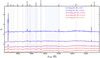Fig. A.1.

Resulting median composite spectra normalized at 4150−4300 Å and associated error (solid line + shaded region) in stellar mass bins (low to high stellar mass from top to bottom). We apply a vertical offset for visualization purposes. We highlight the strongest features that we see in our spectra with vertical lines. The light grey vertical stripes show the spectral ranges that we used to compute D_n4000.

In Fig. A.2 we show our findings of the stacked spectra in over-density bins. In terms of the [OII] emission, we find a decreasing line strength from low- to high-density regions (see also PA18). The Hδ line also depends on local density. The absorption strength increases from low to high density, and the emission component decreases.

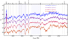Fig. A.2.

Resulting median composite spectra stacks normalized at 4150−4300 Å and associated error (solid line + shaded region) in local over-density bins (low- to high-density regions from top to bottom) for galaxies with stellar masses greater than 10¹⁰ M_⊙. We apply a vertical offset for visualization purposes. We highlight the strongest features that we see in our spectra with vertical lines. The light grey vertical stripes show the spectral ranges that we used to compute D_n4000.

Finally, in Fig. A.3 we show the composite spectra binned by SFR. As expected, the [OII] emission is stronger for high-SFR galaxies. In terms of their Hδ absorption, we see a stronger absorption in higher SFR galaxies.

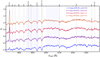Fig. A.3.

Resulting median composite spectra normalized at 4150−4300 Å and associated error (solid line + shaded region) in SFR bins (high to low SFR from top to bottom) for galaxies with stellar masses greater than 10¹⁰ M_⊙. We apply a vertical offset for visualization purposes. We highlight the strongest features that we see in our spectra with vertical lines. The light grey vertical stripes show the spectral ranges that we used to compute D_n4000.

Table A.1.

Summary table with the results for all spectroscopic indices in composite spectra.

All Tables

Table 1.

Results of the linear fits X = m × log₁₀(M_⋆/10¹⁰ M_⊙)+b to EW_[OII] and D_n4000 that are shown in Figs. 6 and 7.

In the text

Table A.1.

Summary table with the results for all spectroscopic indices in composite spectra.

In the text

All Figures

Fig. 1.

Stellar masses and SFRs derived from SED fitting in our spectroscopic sample at 0.8 < z < 0.9, showing the primary (filled circles) and secondary (open circles) targets separately (left). Colour-magnitude diagram for the same sample (right). For comparison, we show the derived best-fit relation for star-forming galaxies computed at z = 0.84 using the equation derived by Whitaker et al. (2012) over a large average volume in the COSMOS field (the dashed line is an extrapolation below their stellar mass completeness). The vertical dotted line shows the approximate stellar-mass representativeness limit of our survey. The dotted contours show the COSMOS2015 distribution of galaxies with 0.8 < z_phot < 0.9 and i_AB < 22.5 from 10% to 90% of the sample in 10% steps.

In the text

Fig. 2.

Number of galaxies with spectroscopic redshifts in VIS³COS divided by the number of galaxies in the mass-complete COSMOS2015 catalogue over the same region and limited to 0.8 < z_phot < 0.9 for all, star-forming, and quiescent galaxies. The vertical dashed lines correspond to the mass-complete limits in COSMOS2015. The vertical dotted lines correspond to our quoted limiting mass of ∼10¹⁰ M_⊙. The error bars are computed from Poisson statistics.

In the text

Fig. 3.

Three examples of the fit to the stacked [O II] emission (left) and the stacked Hδ absorption + emission (right) spectral lines. The solid black line shows the observed spectrum. The green line shows the median fit (after 10 000 realizations), and the orange line is the estimated continuum around the line. We also show in red and blue dashed lines the fit of each Gaussian component.

In the text

Fig. 4.

Value of D_n4000 as a function of stellar age for a set of single stellar population models from Bruzual & Charlot (2003) for different stellar metallicities from Z = 0.1 Z_⊙ to Z = 2.5 Z_⊙. The thick solid line shows the relation using the stellar metallicity for the median stellar mass and redshift of our sample (see Sect. 3.3). Right panel: distribution of measured D_n4000 values for the galaxies in our sample.

In the text

Fig. 5.

Dependence of the three spectral features detailed in Sect. 3.2 (from top to bottom: [OII] EW, Hδ EWs, and D_n4000) as a function of stellar mass (left), over-density (middle), and SED-derived SFR (right). We show our stellar mass representativeness limit as a vertical dotted line in the left panels and show as empty symbols the measurements for which the completeness effects are large. We note that for bins that are not defined in stellar mass (middle and right panels), the composite spectra are built from galaxies with stellar mass greater than 10¹⁰ M_⊙. Results from this paper are shown as large symbols connected by a dotted line with associated error bars derived from the 16th and 84th percentiles of the 1000 bootstrapped fits (when the error bars are not shown, it implies an error smaller than the symbol size). The trends with stellar mass show a decrease in [OII] and Hδ emission (blue squares) and absorption (red circles) strength and an increase in the average age of the stellar population (traced by D_n4000). The trends with over-density show a peak in [OII] EW at filament-like densities, and Hδ EWs show little dependence on local density. There is also a clear trend that galaxies are older in higher density regions. Lastly, the strength of [OII] and Hδ increases with SFR (except for the most strongly star-forming galaxies), and younger populations lie in galaxies with higher SFR, as expected. We compare our results to other surveys in the literature (Bridge et al. 2015; Darvish et al. 2015a; Cava et al. 2015; Wu et al. 2018; Hernán-Caballero et al. 2013; Vergani et al. 2008; Muzzin et al. 2012). For a more detailed discussion of the differences, we refer to Sects. 4.2.1 and 4.2.2.

In the text

Fig. 6.

Relation between [OII] EW and stellar mass for the [OII]-emitters in our sample in three different over-density bins. We compare our results (large green and dark blue symbols are the median of the population, and the same smaller symbols represent individual measurements) with results from Darvish et al. (2015a) of filament and field galaxies, as small red and blue triangles, respectively. We show the best fit (with error estimate) from Eq. (5) for each density bin as shaded regions. We show that higher stellar mass galaxies have weaker [OII] emission, and this relation is seen in all over-density subsets.

In the text

Fig. 7.

D_n4000 as a function of stellar mass for three different over-density bins. The vertical dotted line shows the representativeness limit of our survey. We show the best fit (with errors) from Eq. (6) for each density bin as shaded regions. We find an underlying correlation between stellar masses and D_n4000: the median D_n4000 of galaxies in high-density regions is higher than in low-density regions. The difference between low- and high-density environments is larger at higher stellar masses. We compare with the results from GCLASS (Muzzin et al. 2012), from VVDS (Vergani et al. 2008), from SHARDS (Hernán-Caballero et al. 2013), and from LEGA-C (Wu et al. 2018), which also show the same trends. We also show here the median value of D_n4000 as a function of both stellar mass and local density in in the right panel. This map is a smooth interpolation of the trends found in our sample and highlights the increase of the median D_n4000 with increasing stellar mass and local density.

In the text

	Fig. 8. Dependence of the three spectral indices detailed in Sect. 3.2 (from top to bottom: [OII] EW, Hδ EW, and D_n4000) as a function of over-density in three stellar mass bins. This highlights the impact of stellar mass and environment on the observed spectral properties of galaxies.
In the text

Fig. 9.

Observed relation between D_n4000 and log₁₀(−EW_[OII]) for individual galaxies (small symbols) and median per stellar mass bin (large symbols), colour-coded by their stellar mass. The small purple dots show the values for galaxies with log₁₀(M_⋆/M_⊙) < 10. Different symbols correspond to different over-densities. The dashed lines are linear fits to the data of individual galaxies in two stellar mass sub-samples (see text for details): the steeper slope is the fit for galaxies with 10 < log₁₀(M_⋆/M_⊙) < 11, and the shallower slope is the fit for galaxies with log₁₀(M_⋆/M_⊙) > 11. This highlights the underlying anti-correlation between the observed strength of the [OII] emission and the strength of the 4000 Å break. We show as a black contour the location of 85% of the zCOSMOS sample at 0.48 < z < 1.2 with stellar masses greater than 10¹⁰ M_⊙ (Vergani et al. 2010).

In the text

Fig. 10.

Properties of composite spectra of quiescent and star-forming galaxies selected according to their sSFR (separation at log₁₀(sSFR) = − 11, see also PA18) in low- (diamonds) and high-density regions (squares). The dotted lines are for D_n4000 = 1.325 and EW_[OII] = 4 Å and are shown to guide the eye. These two populations are separated in D_n4000 and EW_[OII], and some environmental effects can also be found within each population of galaxies. Quiescent and star-forming populations are more clearly separated in high-density regions.

In the text

Fig. A.1.

Resulting median composite spectra normalized at 4150−4300 Å and associated error (solid line + shaded region) in stellar mass bins (low to high stellar mass from top to bottom). We apply a vertical offset for visualization purposes. We highlight the strongest features that we see in our spectra with vertical lines. The light grey vertical stripes show the spectral ranges that we used to compute D_n4000.

In the text

Fig. A.2.

Resulting median composite spectra stacks normalized at 4150−4300 Å and associated error (solid line + shaded region) in local over-density bins (low- to high-density regions from top to bottom) for galaxies with stellar masses greater than 10¹⁰ M_⊙. We apply a vertical offset for visualization purposes. We highlight the strongest features that we see in our spectra with vertical lines. The light grey vertical stripes show the spectral ranges that we used to compute D_n4000.

In the text

Fig. A.3.

Resulting median composite spectra normalized at 4150−4300 Å and associated error (solid line + shaded region) in SFR bins (high to low SFR from top to bottom) for galaxies with stellar masses greater than 10¹⁰ M_⊙. We apply a vertical offset for visualization purposes. We highlight the strongest features that we see in our spectra with vertical lines. The light grey vertical stripes show the spectral ranges that we used to compute D_n4000.

In the text

Current usage metrics show cumulative count of Article Views (full-text article views including HTML views, PDF and ePub downloads, according to the available data) and Abstracts Views on Vision4Press platform.

Data correspond to usage on the plateform after 2015. The current usage metrics is available 48-96 hours after online publication and is updated daily on week days.

Initial download of the metrics may take a while.

[1] Aragón-Calvo, M. A., van de Weygaert, R., & Jones, B. J. T. 2010, MNRAS, 408, 2163 [NASA ADS] [CrossRef] [Google Scholar]

[2] Astropy Collaboration (Robitaille, T. P., et al.) 2013, A&A, 558, A33 [NASA ADS] [CrossRef] [EDP Sciences] [Google Scholar]

[3] Bahé, Y. M., McCarthy, I. G., Balogh, M. L., & Font, A. S. 2013, MNRAS, 430, 3017 [NASA ADS] [CrossRef] [Google Scholar]

[4] Balogh, M. L., Morris, S. L., Yee, H. K. C., Carlberg, R. G., & Ellingson, E. 1999, ApJ, 527, 54 [NASA ADS] [CrossRef] [Google Scholar]

[5] Balogh, M. L., Navarro, J. F., & Morris, S. L. 2000, ApJ, 540, 113 [NASA ADS] [CrossRef] [Google Scholar]

[6] Bekki, K. 2009, MNRAS, 399, 2221 [NASA ADS] [CrossRef] [Google Scholar]

[7] Belfiore, F., Maiolino, R., Maraston, C., et al. 2016, MNRAS, 461, 3111 [Google Scholar]

[8] Belfiore, F., Maiolino, R., Maraston, C., et al. 2017, MNRAS, 466, 2570 [NASA ADS] [CrossRef] [Google Scholar]

[9] Best, P. N. 2004, MNRAS, 351, 70 [NASA ADS] [CrossRef] [Google Scholar]

[10] Birnboim, Y., & Dekel, A. 2003, MNRAS, 345, 349 [NASA ADS] [CrossRef] [Google Scholar]

[11] Birnboim, Y., Dekel, A., & Neistein, E. 2007, MNRAS, 380, 339 [NASA ADS] [CrossRef] [Google Scholar]

[12] Blanton, M. R., Eisenstein, D., Hogg, D. W., Schlegel, D. J., & Brinkmann, J. 2005, ApJ, 629, 143 [NASA ADS] [CrossRef] [Google Scholar]

[13] Boselli, A., Roehlly, Y., Fossati, M., et al. 2016, A&A, 596, A11 [NASA ADS] [CrossRef] [EDP Sciences] [Google Scholar]

[14] Bower, R. G., Benson, A. J., Malbon, R., et al. 2006, MNRAS, 370, 645 [NASA ADS] [CrossRef] [Google Scholar]

[15] Bridge, J. S., Gronwall, C., Ciardullo, R., et al. 2015, ApJ, 799, 205 [NASA ADS] [CrossRef] [Google Scholar]

[16] Bruzual, A. G. 1983, ApJ, 273, 105 [NASA ADS] [CrossRef] [Google Scholar]

[17] Bruzual, G., & Charlot, S. 2003, MNRAS, 344, 1000 [NASA ADS] [CrossRef] [Google Scholar]

[18] Calzetti, D., Armus, L., Bohlin, R. C., et al. 2000, ApJ, 533, 682 [NASA ADS] [CrossRef] [Google Scholar]

[19] Cava, A., Pérez-González, P. G., Eliche-Moral, M. C., et al. 2015, ApJ, 812, 155 [NASA ADS] [CrossRef] [Google Scholar]

[20] Chabrier, G. 2003, ApJ, 586, L133 [NASA ADS] [CrossRef] [Google Scholar]

[21] Charlot, S., & Fall, S. M. 2000, ApJ, 539, 718 [NASA ADS] [CrossRef] [Google Scholar]

[22] Cohen, S. A., Hickox, R. C., Wegner, G. A., Einasto, M., & Vennik, J. 2017, ApJ, 835, 56 [NASA ADS] [CrossRef] [Google Scholar]

[23] Combes, F., García-Burillo, S., Braine, J., et al. 2013, A&A, 550, A41 [NASA ADS] [CrossRef] [EDP Sciences] [Google Scholar]

[24] Cooke, E. A., Smail, I., Stach, S. M., et al. 2019, MNRAS, 486, 3047 [NASA ADS] [CrossRef] [Google Scholar]

[25] Cooper, M. C., Tremonti, C. A., Newman, J. A., & Zabludoff, A. I. 2008, MNRAS, 390, 245 [NASA ADS] [CrossRef] [Google Scholar]

[26] Coppin, K. E. K., Geach, J. E., Webb, T. M. A., et al. 2012, ApJ, 749, L43 [NASA ADS] [CrossRef] [Google Scholar]

[27] Couch, W. J., & Sharples, R. M. 1987, MNRAS, 229, 423 [NASA ADS] [CrossRef] [Google Scholar]

[28] Cox, T. J., Jonsson, P., Primack, J. R., & Somerville, R. S. 2006, MNRAS, 373, 1013 [NASA ADS] [CrossRef] [Google Scholar]

[29] Croton, D. J., Springel, V., White, S. D. M., et al. 2006, MNRAS, 365, 11 [NASA ADS] [CrossRef] [Google Scholar]

[30] Cucciati, O., Iovino, A., Marinoni, C., et al. 2006, A&A, 458, 39 [NASA ADS] [CrossRef] [EDP Sciences] [Google Scholar]

[31] Cucciati, O., Iovino, A., Kovač, K., et al. 2010, A&A, 524, A2 [NASA ADS] [CrossRef] [EDP Sciences] [Google Scholar]

[32] da Cunha, E., Charlot, S., & Elbaz, D. 2008, MNRAS, 388, 1595 [NASA ADS] [CrossRef] [Google Scholar]

[33] Darvish, B., Sobral, D., Mobasher, B., et al. 2014, ApJ, 796, 51 [NASA ADS] [CrossRef] [Google Scholar]

[34] Darvish, B., Mobasher, B., Sobral, D., et al. 2015a, ApJ, 814, 84 [NASA ADS] [CrossRef] [Google Scholar]

[35] Darvish, B., Mobasher, B., Sobral, D., Scoville, N., & Aragon-Calvo, M. 2015b, ApJ, 805, 121 [NASA ADS] [CrossRef] [Google Scholar]

[36] Darvish, B., Mobasher, B., Sobral, D., et al. 2016, ApJ, 825, 113 [NASA ADS] [CrossRef] [Google Scholar]

[37] Darvish, B., Mobasher, B., Martin, D. C., et al. 2017, ApJ, 837, 16 [NASA ADS] [CrossRef] [Google Scholar]

[38] Darvish, B., Martin, C., Gonçalves, T. S., et al. 2018, ApJ, 853, 155 [NASA ADS] [CrossRef] [Google Scholar]

[39] Davidzon, I., Cucciati, O., Bolzonella, M., et al. 2016, A&A, 586, A23 [NASA ADS] [CrossRef] [EDP Sciences] [Google Scholar]

[40] De Rossi, M. E., Bower, R. G., Font, A. S., Schaye, J., & Theuns, T. 2017, MNRAS, 472, 3354 [NASA ADS] [CrossRef] [Google Scholar]

[41] Dekel, A., & Cox, T. J. 2006, MNRAS, 370, 1445 [NASA ADS] [CrossRef] [Google Scholar]

[42] Dressler, A. 1980, ApJ, 236, 351 [NASA ADS] [CrossRef] [Google Scholar]

[43] Dressler, A., Oemler, Jr., A., Poggianti, B. M., et al. 2004, ApJ, 617, 867 [NASA ADS] [CrossRef] [Google Scholar]

[44] Efstathiou, G. 2000, MNRAS, 317, 697 [NASA ADS] [CrossRef] [Google Scholar]

[45] Elbaz, D., Daddi, E., Le Borgne, D., et al. 2007, A&A, 468, 33 [NASA ADS] [CrossRef] [EDP Sciences] [Google Scholar]

[46] Ellison, S. L., Patton, D. R., Simard, L., & McConnachie, A. W. 2008, AJ, 135, 1877 [NASA ADS] [CrossRef] [Google Scholar]

[47] Ellison, S. L., Simard, L., Cowan, N. B., et al. 2009, MNRAS, 396, 1257 [NASA ADS] [CrossRef] [Google Scholar]

[48] Erfanianfar, G., Popesso, P., Finoguenov, A., et al. 2016, MNRAS, 455, 2839 [NASA ADS] [CrossRef] [Google Scholar]

[49] Fabian, A. C. 2012, ARA&A, 50, 455 [NASA ADS] [CrossRef] [Google Scholar]

[50] Finoguenov, A., Guzzo, L., Hasinger, G., et al. 2007, ApJS, 172, 182 [NASA ADS] [CrossRef] [Google Scholar]

[51] Foltz, R., Wilson, G., Muzzin, A., et al. 2018, ApJ, 866, 136 [NASA ADS] [CrossRef] [Google Scholar]

[52] Fritz, J., Poggianti, B. M., Cava, A., et al. 2014, A&A, 566, A32 [NASA ADS] [CrossRef] [EDP Sciences] [Google Scholar]

[53] Fujita, Y. 1998, ApJ, 509, 587 [NASA ADS] [CrossRef] [Google Scholar]

[54] Gabor, J. M., Davé, R., Finlator, K., & Oppenheimer, B. D. 2010, MNRAS, 407, 749 [NASA ADS] [CrossRef] [Google Scholar]

[55] Gallazzi, A., Charlot, S., Brinchmann, J., White, S. D. M., & Tremonti, C. A. 2005, MNRAS, 362, 41 [NASA ADS] [CrossRef] [Google Scholar]

[56] Gallazzi, A., Bell, E. F., Wolf, C., et al. 2009a, ApJ, 690, 1883 [NASA ADS] [CrossRef] [Google Scholar]

[57] Gallazzi, A., Bell, E. F., Wolf, C., et al. 2009b, ApJ, 690, 1883 [NASA ADS] [CrossRef] [Google Scholar]

[58] Geach, J. E., Smail, I., Moran, S. M., Treu, T., & Ellis, R. S. 2009, ApJ, 691, 783 [NASA ADS] [CrossRef] [Google Scholar]

[59] Gomes, J. M., Papaderos, P., Vílchez, J. M., et al. 2016, A&A, 585, A92 [NASA ADS] [CrossRef] [EDP Sciences] [Google Scholar]

[60] Gunn, J. E., & Gott, III., J. R. 1972, ApJ, 176, 1 [NASA ADS] [CrossRef] [Google Scholar]

[61] Haines, C. P., Pereira, M. J., Smith, G. P., et al. 2015, ApJ, 806, 101 [NASA ADS] [CrossRef] [Google Scholar]

[62] Harrison, C. D., Colless, M., Kuntschner, H., et al. 2011, MNRAS, 413, 1036 [NASA ADS] [CrossRef] [Google Scholar]

[63] Hernán-Caballero, A., Alonso-Herrero, A., Pérez-González, P. G., et al. 2013, MNRAS, 434, 2136 [NASA ADS] [CrossRef] [Google Scholar]

[64] Hunter, J. D. 2007, Comput. Sci. Eng., 9, 90 [NASA ADS] [CrossRef] [Google Scholar]

[65] Ideue, Y., Nagao, T., Taniguchi, Y., et al. 2009, ApJ, 700, 971 [NASA ADS] [CrossRef] [Google Scholar]

[66] Ilbert, O., Capak, P., Salvato, M., et al. 2009, ApJ, 690, 1236 [NASA ADS] [CrossRef] [Google Scholar]

[67] Ilbert, O., McCracken, H. J., Le Fèvre, O., et al. 2013, A&A, 556, A55 [NASA ADS] [CrossRef] [EDP Sciences] [Google Scholar]

[68] Iovino, A., Cucciati, O., Scodeggio, M., et al. 2010, A&A, 509, A40 [NASA ADS] [CrossRef] [EDP Sciences] [Google Scholar]

[69] Jaffé, Y. L., Smith, R., Candlish, G. N., et al. 2015, MNRAS, 448, 1715 [NASA ADS] [CrossRef] [Google Scholar]

[70] Jones, E., Oliphant, T., Peterson, P., et al. 2001, SciPy: Open Source Scientific Tools for Python, [Online; accessed 2016–03-23] [Google Scholar]

[71] Kashino, D., Silverman, J. D., Rodighiero, G., et al. 2013, ApJ, 777, L8 [NASA ADS] [CrossRef] [Google Scholar]

[72] Kauffmann, G., Heckman, T. M., White, S. D. M., et al. 2003, MNRAS, 341, 33 [NASA ADS] [CrossRef] [Google Scholar]

[73] Kauffmann, G., White, S. D. M., Heckman, T. M., et al. 2004, MNRAS, 353, 713 [NASA ADS] [CrossRef] [Google Scholar]

[74] Kawinwanichakij, L., Papovich, C., Quadri, R. F., et al. 2017, ApJ, 847, 134 [NASA ADS] [CrossRef] [Google Scholar]

[75] Kennicutt, Jr., R. C. 1998, ARA&A, 36, 189 [Google Scholar]

[76] Kennicutt, R. C., & Evans, N. J. 2012, ARA&A, 50, 531 [NASA ADS] [CrossRef] [Google Scholar]

[77] Kereš, D., Katz, N., Weinberg, D. H., & Davé, R. 2005, MNRAS, 363, 2 [NASA ADS] [CrossRef] [Google Scholar]

[78] Kereš, D., Katz, N., Davé, R., Fardal, M., & Weinberg, D. H. 2009a, MNRAS, 396, 2332 [NASA ADS] [CrossRef] [Google Scholar]

[79] Kereš, D., Katz, N., Fardal, M., Davé, R., & Weinberg, D. H. 2009b, MNRAS, 395, 160 [NASA ADS] [CrossRef] [Google Scholar]

[80] Kewley, L. J., Geller, M. J., & Jansen, R. A. 2004, AJ, 127, 2002 [NASA ADS] [CrossRef] [Google Scholar]

[81] Kewley, L. J., Geller, M. J., & Barton, E. J. 2006, AJ, 131, 2004 [NASA ADS] [CrossRef] [Google Scholar]

[82] Khochfar, S., & Burkert, A. 2003, ApJ, 597, L117 [NASA ADS] [CrossRef] [Google Scholar]

[83] Khochfar, S., & Silk, J. 2009, MNRAS, 397, 506 [NASA ADS] [CrossRef] [Google Scholar]

[84] Kocevski, D. D., Lemaux, B. C., Lubin, L. M., et al. 2011, ApJ, 737, L38 [NASA ADS] [CrossRef] [Google Scholar]

[85] Kodama, T., Smail, I., Nakata, F., Okamura, S., & Bower, R. G. 2001, ApJ, 562, L9 [Google Scholar]

[86] Kodama, T., Balogh, M. L., Smail, I., Bower, R. G., & Nakata, F. 2004, MNRAS, 354, 1103 [NASA ADS] [CrossRef] [Google Scholar]

[87] Kormendy, J. 2013, in Secular Evolution in Disk Galaxies, eds. J. Falcón-Barroso, & J. H. Knapen, 1 [Google Scholar]

[88] Koyama, Y., Kodama, T., Shimasaku, K., et al. 2008, MNRAS, 391, 1758 [NASA ADS] [CrossRef] [Google Scholar]

[89] Koyama, Y., Kodama, T., Shimasaku, K., et al. 2010, MNRAS, 403, 1611 [NASA ADS] [CrossRef] [Google Scholar]

[90] Koyama, Y., Smail, I., Kurk, J., et al. 2013, MNRAS, 434, 423 [NASA ADS] [CrossRef] [Google Scholar]

[91] Laigle, C., McCracken, H. J., Ilbert, O., et al. 2016, ApJS, 224, 24 [NASA ADS] [CrossRef] [Google Scholar]

[92] Larson, R. B., Tinsley, B. M., & Caldwell, C. N. 1980, ApJ, 237, 692 [NASA ADS] [CrossRef] [Google Scholar]

[93] Leethochawalit, N., Kirby, E. N., Moran, S. M., Ellis, R. S., & Treu, T. 2018, ApJ, 856, 15 [NASA ADS] [CrossRef] [Google Scholar]

[94] Lehnert, M. D., Le Tiran, L., Nesvadba, N. P. H., et al. 2013, A&A, 555, A72 [NASA ADS] [CrossRef] [EDP Sciences] [Google Scholar]

[95] Lemaux, B. C., Lubin, L. M., Shapley, A., et al. 2010, ApJ, 716, 970 [NASA ADS] [CrossRef] [Google Scholar]

[96] Lemaux, B. C., Tomczak, A. R., Lubin, L. M., et al. 2019, MNRAS, 490, 1231 [NASA ADS] [CrossRef] [Google Scholar]

[97] Lewis, I., Balogh, M., De Propris, R., et al. 2002, MNRAS, 334, 673 [NASA ADS] [CrossRef] [Google Scholar]

[98] Li, C., Kauffmann, G., Jing, Y. P., et al. 2006, MNRAS, 368, 21 [NASA ADS] [CrossRef] [Google Scholar]

[99] Li, I. H., Yee, H. K. C., & Ellingson, E. 2009, ApJ, 698, 83 [NASA ADS] [CrossRef] [Google Scholar]

[100] Li, I. H., Glazebrook, K., Gilbank, D., et al. 2011, MNRAS, 411, 1869 [NASA ADS] [CrossRef] [Google Scholar]

[101] Lin, L., Cooper, M. C., Jian, H.-Y., et al. 2010, ApJ, 718, 1158 [NASA ADS] [CrossRef] [Google Scholar]

[102] Ma, X., Hopkins, P. F., Faucher-Giguère, C.-A., et al. 2016, MNRAS, 456, 2140 [NASA ADS] [CrossRef] [Google Scholar]

[103] Madau, P., & Dickinson, M. 2014, ARA&A, 52, 415 [NASA ADS] [CrossRef] [Google Scholar]

[104] Malavasi, N., Arnouts, S., Vibert, D., et al. 2017, MNRAS, 465, 3817 [NASA ADS] [CrossRef] [EDP Sciences] [Google Scholar]

[105] Mancone, C. L., & Gonzalez, A. H. 2012, PASP, 124, 606 [NASA ADS] [CrossRef] [Google Scholar]

[106] Mansheim, A. S., Lemaux, B. C., Tomczak, A. R., et al. 2017a, MNRAS, 469, L20 [NASA ADS] [CrossRef] [Google Scholar]

[107] Mansheim, A. S., Lemaux, B. C., Dawson, W. A., et al. 2017b, ApJ, 834, 205 [NASA ADS] [CrossRef] [Google Scholar]

[108] Martin, D. C., Gonçalves, T. S., Darvish, B., Seibert, M., & Schiminovich, D. 2017, ApJ, 842, 20 [NASA ADS] [CrossRef] [Google Scholar]

[109] Masters, D., & Capak, P. 2011, PASP, 123, 638 [NASA ADS] [CrossRef] [Google Scholar]

[110] McIntosh, D. H., Guo, Y., Hertzberg, J., et al. 2008, MNRAS, 388, 1537 [NASA ADS] [CrossRef] [Google Scholar]

[111] Merritt, D. 1984, ApJ, 276, 26 [NASA ADS] [CrossRef] [Google Scholar]

[112] Mihos, J. C., & Hernquist, L. 1996, ApJ, 464, 641 [NASA ADS] [CrossRef] [Google Scholar]

[113] Moore, B., Lake, G., & Katz, N. 1998, ApJ, 495, 139 [NASA ADS] [CrossRef] [Google Scholar]

[114] Mosleh, M., Tavasoli, S., & Tacchella, S. 2018, ApJ, 861, 101 [NASA ADS] [CrossRef] [Google Scholar]

[115] Moss, C. 2006, MNRAS, 373, 167 [NASA ADS] [CrossRef] [Google Scholar]

[116] Muzzin, A., Wilson, G., Yee, H. K. C., et al. 2012, ApJ, 746, 188 [NASA ADS] [CrossRef] [Google Scholar]

[117] Nantais, J. B., Rettura, A., Lidman, C., et al. 2013, A&A, 556, A112 [NASA ADS] [CrossRef] [EDP Sciences] [Google Scholar]

[118] Nelan, J. E., Smith, R. J., Hudson, M. J., et al. 2005, ApJ, 632, 137 [NASA ADS] [CrossRef] [Google Scholar]

[119] Oemler, Jr., A. 1974, ApJ, 194, 1 [NASA ADS] [CrossRef] [Google Scholar]

[120] Oemler, Jr., A., Dressler, A., Kelson, D., et al. 2009, ApJ, 693, 152 [NASA ADS] [CrossRef] [Google Scholar]

[121] Oke, J. B., & Gunn, J. E. 1983, ApJ, 266, 713 [NASA ADS] [CrossRef] [Google Scholar]

[122] Owers, M. S., Couch, W. J., Nulsen, P. E. J., & Randall, S. W. 2012, ApJ, 750, L23 [NASA ADS] [CrossRef] [Google Scholar]

[123] Pannella, M., Elbaz, D., Daddi, E., et al. 2015, ApJ, 807, 141 [NASA ADS] [CrossRef] [Google Scholar]

[124] Patel, S. G., Holden, B. P., Kelson, D. D., Illingworth, G. D., & Franx, M. 2009, ApJ, 705, L67 [NASA ADS] [CrossRef] [Google Scholar]

[125] Paulino-Afonso, A., Sobral, D., Darvish, B., et al. 2018, A&A, 620, A186 [NASA ADS] [CrossRef] [EDP Sciences] [Google Scholar]

[126] Peng, Y.-J., Lilly, S. J., Kovač, K., et al. 2010a, ApJ, 721, 193 [NASA ADS] [CrossRef] [Google Scholar]

[127] Peng, C. Y., Ho, L. C., Impey, C. D., & Rix, H.-W. 2010b, AJ, 139, 2097 [NASA ADS] [CrossRef] [Google Scholar]

[128] Peng, Y.-J., Lilly, S. J., Renzini, A., & Carollo, M. 2012, ApJ, 757, 4 [NASA ADS] [CrossRef] [Google Scholar]

[129] Perez, J., Tissera, P., Padilla, N., Alonso, M. S., & Lambas, D. G. 2009, MNRAS, 399, 1157 [NASA ADS] [CrossRef] [Google Scholar]

[130] Poggianti, B. M., & Barbaro, G. 1997, A&A, 325, 1025 [NASA ADS] [Google Scholar]

[131] Poggianti, B. M., Smail, I., Dressler, A., et al. 1999, ApJ, 518, 576 [NASA ADS] [CrossRef] [Google Scholar]

[132] Poggianti, B. M., von der Linden, A., De Lucia, G., et al. 2006, ApJ, 642, 188 [NASA ADS] [CrossRef] [Google Scholar]

[133] Poggianti, B. M., Aragón-Salamanca, A., Zaritsky, D., et al. 2009, ApJ, 693, 112 [NASA ADS] [CrossRef] [Google Scholar]

[134] Poggianti, B. M., Fasano, G., Omizzolo, A., et al. 2016, AJ, 151, 78 [Google Scholar]

[135] Popesso, P., Rodighiero, G., Saintonge, A., et al. 2011, A&A, 532, A145 [NASA ADS] [CrossRef] [EDP Sciences] [Google Scholar]

[136] Puchwein, E., & Springel, V. 2013, MNRAS, 428, 2966 [NASA ADS] [CrossRef] [Google Scholar]

[137] Rettura, A., Rosati, P., Nonino, M., et al. 2010, ApJ, 709, 512 [NASA ADS] [CrossRef] [Google Scholar]

[138] Rettura, A., Mei, S., Stanford, S. A., et al. 2011, ApJ, 732, 94 [NASA ADS] [CrossRef] [Google Scholar]

[139] Roediger, E., Brüggen, M., Owers, M. S., Ebeling, H., & Sun, M. 2014, MNRAS, 443, L114 [NASA ADS] [CrossRef] [Google Scholar]

[140] Salim, S., Rich, R. M., Charlot, S., et al. 2007, ApJS, 173, 267 [NASA ADS] [CrossRef] [Google Scholar]

[141] Santos, J. S., Altieri, B., Popesso, P., et al. 2013, MNRAS, 433, 1287 [NASA ADS] [CrossRef] [Google Scholar]

[142] Santos, J. S., Altieri, B., Tanaka, M., et al. 2014, MNRAS, 438, 2565 [NASA ADS] [CrossRef] [Google Scholar]

[143] Savaglio, S., Glazebrook, K., Le Borgne, D., et al. 2005, ApJ, 635, 260 [NASA ADS] [CrossRef] [Google Scholar]

[144] Scoville, N., Abraham, R. G., Aussel, H., et al. 2007, ApJS, 172, 38 [NASA ADS] [CrossRef] [Google Scholar]

[145] Scoville, N., Arnouts, S., Aussel, H., et al. 2013, ApJS, 206, 3 [NASA ADS] [CrossRef] [Google Scholar]

[146] Singh, R., van de Ven, G., Jahnke, K., et al. 2013, A&A, 558, A43 [NASA ADS] [CrossRef] [EDP Sciences] [Google Scholar]

[147] Siudek, M., Małek, K., Scodeggio, M., et al. 2017, A&A, 597, A107 [NASA ADS] [CrossRef] [EDP Sciences] [Google Scholar]

[148] Smail, I., Morrison, G., Gray, M. E., et al. 1999, ApJ, 525, 609 [NASA ADS] [CrossRef] [Google Scholar]

[149] Sobral, D., Best, P. N., Smail, I., et al. 2011, MNRAS, 411, 675 [NASA ADS] [CrossRef] [Google Scholar]

[150] Sobral, D., Best, P. N., Smail, I., et al. 2014, MNRAS, 437, 3516 [NASA ADS] [CrossRef] [Google Scholar]

[151] Sobral, D., Stroe, A., Dawson, W. A., et al. 2015, MNRAS, 450, 630 [NASA ADS] [CrossRef] [Google Scholar]

[152] Sobral, D., Stroe, A., Koyama, Y., et al. 2016, MNRAS, 458, 3443 [NASA ADS] [CrossRef] [Google Scholar]

[153] Socolovsky, M., Almaini, O., Hatch, N. A., et al. 2018, MNRAS, 476, 1242 [NASA ADS] [CrossRef] [Google Scholar]

[154] Somerville, R. S., Hopkins, P. F., Cox, T. J., Robertson, B. E., & Hernquist, L. 2008, MNRAS, 391, 481 [NASA ADS] [CrossRef] [Google Scholar]

[155] Stach, S. M., Swinbank, A. M., Smail, I., et al. 2017, ApJ, 849, 154 [NASA ADS] [CrossRef] [Google Scholar]

[156] Stroe, A., Sobral, D., Röttgering, H. J. A., & van Weeren, R. J. 2014, MNRAS, 438, 1377 [NASA ADS] [CrossRef] [Google Scholar]

[157] Stroe, A., Sobral, D., Dawson, W., et al. 2015, MNRAS, 450, 646 [NASA ADS] [CrossRef] [Google Scholar]

[158] Stroe, A., Sobral, D., Paulino-Afonso, A., et al. 2017, MNRAS, 465, 2916 [NASA ADS] [CrossRef] [Google Scholar]

[159] Thomas, D., Maraston, C., Bender, R., & Mendes de Oliveira, C. 2005, ApJ, 621, 673 [NASA ADS] [CrossRef] [Google Scholar]

[160] Tomczak, A. R., Lemaux, B. C., Lubin, L. M., et al. 2019, MNRAS, 484, 4695 [Google Scholar]

[161] Tonnesen, S., & Cen, R. 2012, MNRAS, 425, 2313 [NASA ADS] [CrossRef] [Google Scholar]

[162] Tran, K.-V. H., Papovich, C., Saintonge, A., et al. 2010, ApJ, 719, L126 [CrossRef] [Google Scholar]

[163] Tremonti, C. A., Heckman, T. M., Kauffmann, G., et al. 2004, ApJ, 613, 898 [NASA ADS] [CrossRef] [Google Scholar]

[164] van de Voort, F., Bahé, Y. M., Bower, R. G., et al. 2017, MNRAS, 466, 3460 [NASA ADS] [CrossRef] [Google Scholar]

[165] van der Burg, R. F. J., Muzzin, A., Hoekstra, H., et al. 2013, A&A, 557, A15 [NASA ADS] [CrossRef] [EDP Sciences] [Google Scholar]

[166] Vergani, D., Scodeggio, M., Pozzetti, L., et al. 2008, A&A, 487, 89 [NASA ADS] [CrossRef] [EDP Sciences] [Google Scholar]

[167] Vergani, D., Zamorani, G., Lilly, S., et al. 2010, A&A, 509, A42 [NASA ADS] [CrossRef] [EDP Sciences] [Google Scholar]

[168] Walt, S. V. D., Colbert, S. C., & Varoquaux, G. 2011, Comput. Sci. Eng., 13, 22 [Google Scholar]

[169] Wetzel, A. R., Tinker, J. L., Conroy, C., & van den Bosch, F. C. 2013, MNRAS, 432, 336 [NASA ADS] [CrossRef] [Google Scholar]

[170] Whitaker, K. E., van Dokkum, P. G., Brammer, G., & Franx, M. 2012, ApJ, 754, L29 [NASA ADS] [CrossRef] [Google Scholar]

[171] Wild, V., Charlot, S., Brinchmann, J., et al. 2011, MNRAS, 417, 1760 [NASA ADS] [CrossRef] [Google Scholar]

[172] Worthey, G., & Ottaviani, D. L. 1997, ApJS, 111, 377 [NASA ADS] [CrossRef] [Google Scholar]

[173] Wu, P.-F., Zahid, H. J., Hwang, H. S., & Geller, M. J. 2017, MNRAS, 468, 1881 [NASA ADS] [CrossRef] [Google Scholar]

[174] Wu, P.-F., van der Wel, A., Gallazzi, A., et al. 2018, ApJ, 855, 85 [NASA ADS] [CrossRef] [Google Scholar]

[175] Wuyts, S., Förster Schreiber, N. M., Lutz, D., et al. 2011, ApJ, 738, 106 [NASA ADS] [CrossRef] [Google Scholar]

[176] Yan, R., Newman, J. A., Faber, S. M., et al. 2006, ApJ, 648, 281 [NASA ADS] [CrossRef] [Google Scholar]

[177] Zahid, H. J., Kewley, L. J., & Bresolin, F. 2011, ApJ, 730, 137 [NASA ADS] [CrossRef] [Google Scholar]

[178] Zahid, H. J., Geller, M. J., Kewley, L. J., et al. 2013, ApJ, 771, L19 [NASA ADS] [CrossRef] [Google Scholar]

III. Environmental effects on the star formation histories of galaxies at z ∼ 0.8 seen in [O II], Hδ, and Dn4000⋆⋆⋆

1. Introduction

2. VIS3COS survey

2.1. Survey description

2.2. Completeness corrections

3. Spectroscopic properties

3.1. Composite spectra

3.2. Spectral quantities

3.2.1. [OII] emission

3.2.2. Hδ in emission and absorption

3.2.3. Continuum and error estimation

3.2.4. 4000 Å break

3.3. Stellar population age estimates

4. Results

4.1. Global trends on the spectroscopic properties

4.1.1. Stellar mass

4.1.2. Local environment

4.1.3. Star formation rate

4.2. Distinguishing environment and stellar mass effects

4.2.1. EW[OII]

4.2.2. 4000 Å break

4.2.3. Hδ emission and absorption

4.2.4. Anti-correlation between Dn4000 and EW[OII]

4.3. Star formation activity in different environments

5. Discussion

5.1. Environmental effects on star formation

5.2. Older population prevalence influenced by the environment

6. Conclusions

Acknowledgments

References

Appendix A: Detailed spectral stack results

All Tables

All Figures

VIS³COS

III. Environmental effects on the star formation histories of galaxies at z ∼ 0.8 seen in [O II], Hδ, and D_n4000^⋆^⋆⋆

2. VIS³COS survey

4.2.1. EW_[OII]

4.2.4. Anti-correlation between D_n4000 and EW_[OII]