| Issue |
A&A
Volume 696, April 2025
|
|
|---|---|---|
| Article Number | A116 | |
| Number of page(s) | 11 | |
| Section | Extragalactic astronomy | |
| DOI | https://doi.org/10.1051/0004-6361/202453620 | |
| Published online | 09 April 2025 | |
The COSMOS Wall at z ∼ 0.73: Quiescent galaxies and their evolution in different environments⋆
1
Università degli Studi di Milano-Bicocca, Piazza della Scienza, I-20125 Milano, Italy
2
INAF-Osservatorio Astronomico di Brera, Via Brera 28, I-20121 Milano, Italy
3
INAF – Osservatorio di Astrofisica e Scienza dello Spazio di Bologna, Via Gobetti 93/3, I-40129 Bologna, Italy
4
Department of Physics, University of Helsinki, Gustaf Hällströmin katu 2, 00560 Helsinki, Finland
5
Max Planck Institute for Extraterrestrial Physics, Giessenbachstr. 1, 85748 Garching, Germany
6
INAF – IASF Milano, Via Bassini 15, I-20133 Milano, Italy
7
Laboratoire d’Astrophysique de Marseille, CNRS-Université d’Aix-Marseille, 38 Rue F. Joliot Curie, F-13388 Marseille, France
⋆⋆ Corresponding author; This email address is being protected from spambots. You need JavaScript enabled to view it.
Received:
27
December
2024
Accepted:
13
March
2025
Abstract
The evolution of quiescent galaxies is driven by numerous physical processes, often considered to be related to their stellar mass and environment over cosmic time. Tracing their stellar populations can provide insight into the processes that transformed these galaxies into their observed quiescent state. In particular, higher-redshift galaxies, being younger, exhibit more pronounced relative age differences. At early stages, even small differences in age remain significant, whereas as galaxies evolve, these differences become less detectable, making it harder to trace the impact of environmental effects in the local Universe. The COSMOS Wall is a structure at z ∼ 0.73 that contains a large variety of environments, from rich and dense clusters down to field-like regions. Thus, this sample offers a great opportunity to study the effect of the environment on the quiescent galaxy population. Leveraging high-quality spectroscopic data from the LEGA-C survey, combined with the extensive photometric coverage of the COSMOS2020 catalogue, we performed a full-index and photometry fitting of 74 massive (log M⋆/M⊙ = 10.47) quiescent galaxies, deriving their mass-weighted ages, metallicities, and star formation timescales. We characterised the environment in three subsamples: X-ray- and non-X-ray-detected groups and a lower-density subsample similar to the average field. We find a decreasing trend in mass-weighted age with increasing environmental density, with galaxies groups ≳1 Gyr older than those in the field. Conversely, we do not find any significant difference in stellar metallicity between galaxies in X-ray and non-X-ray groups, while we find galaxies with 0.15 dex higher metallicities in the field. Our results indicate that, at z ∼ 0.7, the environment plays a crucial role in shaping the evolution of massive quiescent galaxies, noticeably affecting both their mass-weighted age and star formation timescale. These results support faster quenching mechanisms, at fixed stellar mass, in the dense X-ray-detected groups compared to the field.
Key words: galaxies: abundances / galaxies: evolution / galaxies: formation / galaxies: high-redshift / galaxies: stellar content
Based on observations made with ESO Telescopes at the European Southern Observatory, Cerro Paranal, Chile, under program IDs 194-A.2005 and 1100.A-0949 (The LEGA-C Public Spectroscopy Survey), and ESO 085.A-0664 (The cosmos structure at z = 0.73: exploring the onset of environment-driven trends).
© The Authors 2025
 Open Access article, published by EDP Sciences, under the terms of the Creative Commons Attribution License (https://creativecommons.org/licenses/by/4.0), which permits unrestricted use, distribution, and reproduction in any medium, provided the original work is properly cited.
This article is published in open access under the Subscribe to Open model. This email address is being protected from spambots. You need JavaScript enabled to view it. to support open access publication.
1. Introduction
Determining the efficiency of and interplay between the different physical mechanisms leading to galaxy quenching is still one of the unsolved problems in galaxy evolution. Several processes can contribute to the suppression of star formation, and they can be grouped in two broad classes: those related to the galaxy properties (internal processes) and those related to the environment in which galaxies reside (external processes). The efficiency of internal processes increases with galaxy mass, a key property that regulates the physics of mechanisms such as stellar and active galactic nucleus feedback (e.g. Croton et al. 2006; Fabian 2012; Cicone et al. 2014). In contrast, the external processes involve a large variety of mechanisms, including ram-pressure stripping (e.g. Gunn & Gott 1972), strangulation (e.g. Larson et al. 1980; Balogh et al. 2000), and galaxy-galaxy interactions (e.g. Mihos & Hernquist 1996; Moore et al. 1998). Dynamical gas removal processes like ram-pressure stripping, typical in high-density environments (Boselli et al. 2022), can rapidly deplete the cold gas reservoir, leading to a fast quenching event. Conversely, processes that reduce the cosmological gas inflow (e.g. the ‘cosmological starvation’ process presented by Man & Belli 2018), in combination with maintenance mode feedback processes (Davé et al. 2012), can also occur in lower-density environments, or in the field, and potentially have longer quenching times (Man & Belli 2018). This scenario also results in an overall younger and more metal-enriched stellar population with respect to galaxies quenched by faster processes. Although both mass and environmental quenching contribute to the suppression of star formation, their relative significance varies depending on the galaxy mass and the cosmic epoch. Moreover, the effects of these various quenching processes on galaxy properties are often degenerate, making it challenging to distinguish their individual contributions.
Quiescent galaxies are ideal laboratories for performing studies on which mechanisms lead to galaxy quenching since they contain fingerprints of the quenching processes. In particular, the physical properties of quiescent galaxies, such as the age and the metallicity of their stellar populations, can provide strong constraints on timescales and thus the physical origin of the quenching mechanisms. Stellar population properties of quiescent galaxies have been known to vary strongly with the environment in which galaxies are located (Spitzer & Baade 1951; Oemler 1974; Davis & Geller 1976; Dressler 1980). In dense environments and massive haloes, the evolution from star-forming galaxies to quiescent ones takes place sooner than in the field (Cooper et al. 2006; Cucciati et al. 2006; Poggianti et al. 2006; Iovino et al. 2010; Peng et al. 2010). However, whether this environmental signal is merely the result of different galaxy masses in different environments (i.e. the mass segregation framework) or reflects intrinsic differences in stellar history at fixed mass is still debated (e.g. Baldry et al. 2006; Thomas et al. 2010; Poggianti et al. 2013). Studies on the effect of the environment are mainly performed in the context of the local Universe. In particular, the stellar ages and metallicities of quiescent galaxies have been shown to correlate to first order with galaxy mass (e.g. Gallazzi et al. 2005; Thomas et al. 2005, 2010), with environment playing a larger role in less massive galaxies (e.g. Thomas et al. 2010; Gallazzi et al. 2021). Some studies have been able to determine the role of the environment in quiescent galaxies and found older galaxies in the most massive environments with respect to the field (Sánchez-Blázquez et al. 2006).
Thanks to the high-quality spectroscopic data of The Large Early Galaxy Astrophysics Census (LEGA-C) Public Spectroscopic Survey (van der Wel et al. 2016, 2021; Straatman et al. 2018), we are now able to study a large sample of quiescent galaxies at higher redshifts (0.6 < z < 1), where differences in stellar populations could be more pronounced than in the local Universe. The LEGA-C survey targeted galaxies in the Cosmological Evolution Survey (COSMOS) field (Scoville et al. 2007a), in which a prominent large-scale structure was detected in a narrow redshift slice, 0.69 ≤ z ≤ 0.79 (Scoville et al. 2007b; Cassata et al. 2007; Guzzo et al. 2007). This structure, named the COSMOS Wall (Iovino et al. 2016), provides a unique opportunity to investigate the effects of the environment on galaxy evolution. This volume covers a comprehensive range of environments, ranging from a dense cluster to filaments and voids. Moreover, the COSMOS Wall redshift, corresponding to roughly half the age of the Universe (∼6.5 Gyr), marks a transitional period when the Universe’s star formation rate (SFR) was declining and environmental effects began to play a dominant role in shaping galaxy properties (Fossati et al. 2017). For quiescent galaxies specifically, this epoch provides key insights into how and when they ceased star formation, as well as the mechanisms responsible for their transformation.
In this work we present our analysis of the stellar populations of quiescent galaxies in this peculiar field. We assembled a multi-wavelength dataset in order to exploit all the available information. We used a hierarchical Bayesian method to determine the average stellar population parameters for galaxies in different environments. A complementary study (Zhou et al. 2025) will focus on star-forming galaxies in the COSMOS-Wall volume for a parallel analysis.
In Sect. 2 we present the full set of data used to perform our analysis and the definition of the different environments in the COSMOS Wall. In Sect. 3 we describe in detail the procedures adopted to retrieve the stellar population parameters of our selected sample. In Sect. 4 we present the results that we obtained and the discussion of our analysis. Throughout the paper we adopt a standard Λ cold dark matter cosmology with ΩM = 0.286, ΩΛ = 0.714, and H0 = 69.6 km s−1 Mpc−1 (Bennett et al. 2014). Magnitudes are in the AB system (Oke 1974).
2. Data and sample selection
The COSMOS Wall is a volume identified within the COSMOS survey that contains a large variety of environments, from rich and dense clusters (with X-ray detection) to poor and loose groups, down to average field regions (Scoville et al. 2007b). This volume is at redshift 0.69 ≤ z ≤ 0.79, located in the RA–Dec region displayed in Fig. 1 of Iovino et al. (2016). Readers are referred to Iovino et al. (2016) for more details on this structure’s definition. Iovino et al. (2016) performed a detailed mapping of the COSMOS Wall volume using a friends-of-friends algorithm and an iterative procedure to obtain a reliable group catalogue at different spatial scales. The valuable aspect of this structure consists in the opportunity it offers to study the possible differences in the physical properties of galaxies in relation to their environment, at a fixed cosmic epoch.
The COSMOS field has been targeted by several spectroscopic surveys (e.g. Lilly et al. 2007; Coil et al. 2011; Comparat et al. 2015), and among them the LEGA-C survey (van der Wel et al. 2016) provided high signal to noise ratio and high resolution spectra of the more massive galaxies in this area. Indeed the spectra, observed with the Visible Multi-Object Spectrograph (VIMOS) on the Very Large Telescope (VLT), have an average continuum S/N ∼ 20 Å−1, with an instrumental spectral resolution (R ∼ 3500) suitable to study the stellar population properties of galaxies (DR3; van der Wel et al. 2021). In this work we studied the physical properties of a sample of massive quiescent galaxies within the COSMOS Wall volume by combining optical LEGA-C spectra and a set of photometric data covering a large wavelength range. For the photometric data, we used the multi-wavelength photometric COSMOS2020 catalogue (Weaver et al. 2022). In particular, we used the smallest photometric aperture magnitudes available (2 arcsec) measured in u* band from the MegaCam/CFHT images, in the HSC-SSP PDR2 g-, r-, i-, z- and y-band images and in the UltraVISTA DR4 J-, H- and Ks-band Weaver et al. (2022), in order to match the 1 arcsec slit aperture of the LEGA-C observations (van der Wel et al. 2021).
From the entire LEGA-C sample, we selected galaxies that are in the COSMOS Wall volume as defined above, identifying a total of 244 objects. We measured the available star formation indicators ([OII]λ3727, Hδ, Hβ, [OIII]λ5007) using the latest version of the penalised pixel-fitting (pPXF) code (Cappellari & Emsellem 2004; Cappellari 2017, 2023), adopting the E-MILES simple stellar population (SSP) synthesis models (Vazdekis et al. 2016), obtained assuming the BaSTI tracks (Pietrinferni et al. 2004, 2006) and Chabrier (2003) initial mass function (IMF). We then spectroscopically selected a subsample of quiescent galaxy candidates using the following criteria:
-
EW([OIII]λ5007) < 1 Å;
-
EW(Hβ) < 1 Å;
-
EW([OII]λ3727) < 5 Å;
-
EW(Hδ) < 3 Å in absorption.
These criteria are designed to select galaxies with no detectable [OIII]λ5007 and Hβ emission lines and at most a weak [OII]λ3727 emission, which can occur in quiescent galaxies at these redshifts (see Maseda et al. 2021). Additionally, the last criterion, EW(Hδ) < 3 Å in absorption, excludes post-starburst galaxies from our sample, following the definition of Poggianti et al. (2009). Using the above selection criteria, we defined a sample of 99 quiescent galaxies. However, due to the limited and variable rest-frame spectral range, approximately half of the selected sample lacks at least one of the indicators required for this selection. Specifically, among the 99 selected galaxies, 19 have spectra not including the [OII] line, 14 galaxies lack both [OIII] and Hβ, and 9 ones lack only the [OIII]. For these galaxies, we based the selection on the other available indicators. We tested the possible contamination introduced by using a reduced set of criteria using the subsample of 109 out of 244 galaxies for which all the four indicators are available. For example, we performed the selection without considering the [OII] line and then checked the values of [OII] for the selected galaxies. We found that some galaxies would not meet the selection criteria if the [OII] threshold of 5 Å had been applied. This analysis revealed that, in the worst-case scenario, only 5 out of the 99 galaxies in the sample might not satisfy all the selection criteria when the full set of indicators is considered.
Figure 1 shows the rest-frame UVJ diagram of the 244 galaxies observed in the COSMOS Wall volume by the LEGA-C survey (grey points) and our selected quiescent sample (red points). Rest-frame U − V and V − J values are obtained from the LEGA-C photometric parent sample Muzzin et al. (2013). The entire sample of selected galaxies falls within the region of the UVJ diagram associated with quiescent galaxies, as defined by Williams et al. (2009). Specifically, they occupy the region corresponding to older quiescent galaxies, as defined from Whitaker et al. (2013), further supporting the robustness of our selection. We also inspected the spectra of those galaxies that have colours matching those of the quiescent galaxies in the UVJ plane but that were excluded by our spectroscopic selection. We found that their spectra clearly exhibit gas-phase emission lines in those galaxies. Therefore, we consider the spectroscopic criteria we adopted for selecting quiescent galaxies to be solid and trustworthy.
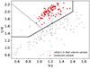 |
Fig. 1. Rest-frame UVJ diagram of the selected sample. The stars are all the galaxies observed in the COSMOS Wall volume by the LEGA-C survey, while the red points mark the spectroscopically selected quiescent galaxies. The solid black line is the separation between star-forming and quiescent galaxies as defined in Eq. (4) of Williams et al. (2009). The dotted line divides younger quiescent galaxies (on the left) and older quiescent galaxies (on the right) according to Whitaker et al. (2013). |
Iovino et al. (2016) classified galaxies in the COSMOS Wall volume as belonging to groups or as field galaxies. Furthermore, by cross-correlating their group catalogue with the list of XMM-COSMOS extended sources presented in George et al. (2011) (down to a limit X-ray detection from of rest-frame log(LX, 0.1 − 2.4 keV/erg s−1)∼41.3, corresponding to log(M200/M⊙) > 13.2), they further categorised the groups into X-ray emitters or non-X-ray emitters. This matching process identified nine groups in the Wall Volume with X-ray detection. Notably, the new X-ray group catalogue for the COSMOS field, derived by Gozaliasl et al. (2019), using combined Chandra and XMM-Newton observations from the COSMOS Legacy Survey, does not alter the list of matched groups originally presented by Iovino et al. (2016). Our sample galaxies can then be divided into three different environment bins: groups with X-ray detection, groups without X-ray detection, and field. Specifically, our sample consists of 22 galaxies located in groups with X-ray detection (hereafter X-ray groups), 28 in groups without X-ray detection (hereafter non-X-ray groups), and 49 in the field.
Figure 2 shows the stellar mass distribution of the galaxies across the three environment bins. We used stellar masses estimated from Muzzin et al. (2013). It is well known that galaxy evolution strongly depends on their stellar mass (e.g. Thomas et al. 2010), and to isolate the effect of environment, we need to compare samples with the same mass distribution across the three environments. According to van der Wel et al. (2021), the LEGA-C sample in the redshift bin between 0.7 and 0.8 is representative down to a stellar mass limit of log M/M⊙ = 10.47. Therefore, we refined our sample selection by restricting it to galaxies within the mass range 10.47 < log M/M⊙ < 11.4, since we used the same measurements from Muzzin et al. (2013). The upper limit was set to exclude the more massive galaxy tail, which is present only in the X-ray group environment. We performed a K-S test for the three distribution in the restricted mass bin, and we obtained a p-value of 0.2 between X-ray and non-X-ray groups, a p-value of 0.4 between X-ray groups and field, and a p-value of 0.5 between non-X-ray groups and field. From the K-S test we did not detect significant differences between the three population and therefore we assumed that the distributions are extracted from the same parent population. Our final sample consists then of 16 galaxies located in X-ray groups, 22 in non-X-ray groups, and 36 in the field, for a total of 74 quiescent galaxies.
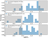 |
Fig. 2. Mass distribution in the three environment bins. The shaded grey region is the mass cut we applied to obtain a homogeneous and representative distribution across the three bins. |
3. Analysis
Our goal is to measure the individual mass-weighted age, the stellar metallicity and the star formation timescale of our sample of quiescent galaxies, and then investigate the effects of the environment on their properties. In this section we describe in detail the steps of the analysis on our sample. Specifically, in Sect. 3.1 we introduce the synthetic templates built to analyse the selected galaxies. In Sect. 3.2 we describe the performed joint fitting of spectra and photometry using Monte Carlo techniques, given the multi-wavelength available data (Sect. 3.2). Finally, we present how we assess the stellar population parameters of each environment bin using the hierarchical Bayesian modelling (Sect. 3.3).
3.1. Stellar population models
We built a set of synthetic templates based on the SSP models from the latest version of the Bruzual & Charlot (2003) library (hereafter the C&B library; see Plat et al. 2019; Sánchez et al. 2022). The SSP models adopt the PARSEC evolutionary tracks (Marigo et al. 2013; Chen et al. 2015). We assumed a Chabrier IMF (Chabrier 2003) with MUP = 100 M⊙ and the MILES stellar library (3540.5 < λ < 7350.2 Å; Sánchez-Blázquez et al. 2006; Falcón-Barroso et al. 2011, 2.5 Å full width at half maximum resolution). The C&B library provides 3300 SSPs unevenly spaced in linear age and [Z/H], covering 220 ages from 0.01 Myr to 14 Gyr and 15 metallicities from [Z/H] = −2.23 to [Z/H] = 0.55 dex; for reference, the solar abundance (Z⊙) is 0.017. From the C&B library we generated composite stellar population templates characterised by a fast rise of star formation, typical of massive quiescent galaxies (e.g. Citro et al. 2016), followed by an exponentially declining star formation history (SFH):
 (1)
(1)
where τ represents the SFR timescale of the SFH, varying between 0.1 ≤ τ ≤ 2 Gyr, in increments of 0.1 Gyr. At t = 2τ the SFR has declined to approximately 30% of its peak value and formed about 75% of the total stellar mass. Finally, we adopted the attenuation law from Calzetti (2001) with 0 ≤ AV ≤ 1 mag. Given the age of the Universe at the redshift of the COSMOS Wall (∼7 Gyr), we set the maximum age of the templates to 8 Gyr.
3.2. Joint spectroscopic and photometric analysis
In our analysis, we combined spectroscopic and photometric data to derive the stellar population parameters of the selected galaxies through comparisons with the spectral template library described in the previous subsection. For each galaxy in the sample, we determined the kinematic parameters (i.e. recession velocity and velocity dispersion) using the latest version of the pPXF code, adopting the template set from the MILES stellar spectral library (Sánchez-Blázquez et al. 2006), convolved to match the LEGA-C instrumental resolution, and considering the rest-frame wavelength range between 3540 Å and 4700 Å. Synthetic templates were then shifted to match the recession velocity of each galaxy and convolved with the estimated stellar velocity dispersion. Our fit of the velocity dispersion are consistent within 10 km/s with the available values from van der Wel et al. (2021).
We then adopted the full-index fitting (FIF) approach (Martín-Navarro et al. 2014) to compare the observed spectra with the synthetic spectral templates. Differently from the more classic index fitting approach, FIF compares the flux within a specific absorption feature (with respect to its continuum value) pixel by pixel rather than averaging it. This pixel-level comparison within the index window is more effective at breaking the degeneracy between age and metallicity compared to the classical index analysis, as it accounts not only for the strength of the absorption feature but also for its detailed shape, which provides additional information about the stellar population parameters (Martín-Navarro et al. 2019; Ditrani et al. 2024). We applied the FIF method to a comprehensive set of spectral indices, namely: Fe3581, Fe3619, Fe3741, Dn4000, FeBand4050, HδF, HγF, Gband4300, Fe4383, and Fe4531 (Gregg 1994; Balogh et al. 1999; Worthey et al. 1994). Given the available wavelength range, we used only Fe indicators to determine the stellar metallicity, meaning that the derived total metallicity is a proxy of the [Fe/H] abundance. Figure 3 shows an example of the FIF approach applied to one of the selected galaxies. The best-fit template closely matches each spectral feature, capturing detailed information from both their depth and pixel-by-pixel shape.
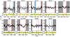 |
Fig. 3. FIF application to the indices available in the LEGA-C ID 209466 galaxy spectrum. The vertical dashed brown lines indicate the feature boundaries for each index, while the grey shaded regions represent the pseudo-continua used for normalisation. In the upper subplots, the black lines and blue shaded regions correspond to the observed spectrum and its associated uncertainty, respectively. The solid red line represents the best-fit derived from the posterior distribution. The green lines in the lower subplots show the residuals between the observed spectrum and the best fit, with the yellow shaded region indicating the relative uncertainties of the observed spectrum. |
The only exception to the FIF approach concerns the Dn4000 index. For this index, we adopted the classic index definition, and its value was compared with the corresponding values measured in the synthetic templates.
Regarding the photometric data, we compared the observed fluxes in the 9 bands described in Sect. 2 with those measured in the same photometric bands on the synthetic spectral templates. For this comparison, we first normalised the synthetic templates using the observed i-band flux corresponding to the wavelength range of the LEGA-C observed spectrum. Additionally, we fitted three ‘jitter’ parameters: lnfuv for the u* band, lnfopt for g-, r-, i-, z- and y-band and lnfir for J-, H- and Ks-band. These parameters act as multiplicative factors applied to the photometric uncertainties in order to balance the likelihoods between the spectroscopic and the photometric fits, given that the S/N of the photometric data significantly exceeds that of the spectroscopic data.
Therefore, we computed the total posterior probability distribution using the likelihood given by ℒ = e−χ2/2, with
 (2)
(2)
where the first term is the contribution of the comparison using the FIF approach, Fsyni is the flux of the synthetic spectrum along the feature of each index, and Fobsi is the flux of the observed spectrum with the error σobsi. The second term is the contribution of the Dn4000 comparison, where Dn4000syn is the index measurement on the synthetic template, and Dn4000obs is the index measurement on the observed spectrum with the error σDn4000obs. Finally, the last term is the contribution of the comparison with the photometric data, where Photsyni is the photometric flux in the i-th band of the synthetic spectrum, and Photobsi is the photometric flux in the i-th band of the observed galaxy with the error σPhotobsi. The photometric error is multiplied by lnfx, where x can be uv, opt, or ir as described above. We derived posterior probability distributions and the Bayesian evidence using the nested sampling Monte Carlo algorithm MLFriends (Buchner 2016, 2019) using the UltraNest1 package (Buchner 2021). We assumed uniform prior for all the parameters considered, summarised in Table 1. Figure 4 shows an example of the joint and marginal probability distributions for all the fitted parameters, while Fig. 5 shows the best-fit applied to both the entire LEGA-C spectrum and the photometric data for a representative quiescent galaxy (LEGA-C ID = 209466). It is evident that our fit provides reasonable fits for both the spectrum and the photometric data of the galaxy.
The seven free parameters fitted to our spectroscopic and photometric data, along with their associated prior distributions.
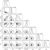 |
Fig. 4. Example of the joint and marginal posterior distributions for the LEGA-C ID 209466 galaxy. Contours represent the 68% and 95% probability levels. The 16%, 50%, and 84% intervals are indicated as dashed lines. |
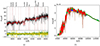 |
Fig. 5. Panel (a), top: Example of the best fit (in red) applied to the entire LEGA-C spectrum of the LEGA-C ID 209466 galaxy (in black). Panel (a), bottom: Difference between the observed spectrum and the best fit, shown in green, and the relative uncertainties of the observed spectrum, shown in yellow. Panel (b): Observed photometric measurements (blue points), best-fitting template (in red), and photometric measurements on the best-fitting template (lime stars). The green shaded region indicates the 68% confidence interval of our posterior. |
3.3. Hierarchical Bayesian modelling
To assess the stellar population parameters in each environment bin, we combined the obtained results for each individual galaxy using the hierarchical Bayesian modelling. In the hierarchical framework, our models consist of two levels: the first level involves the measurements of the parameters for each individual galaxy, while the second level describes how the measurements are distributed within each environment bin. Differently from the classic stacked spectra fit, this approach has several advantages as it avoids introducing correlated noise caused by smoothing the individual spectra to a common velocity dispersion and by the continuum interpolation with polynomials (see Appendix B of Beverage et al. 2023). Following the ‘a posteriori’ approach as in Beverage et al. (2023), as first level of the models we computed the posterior probability distribution of each physical parameter listed in Table 1 for each individual galaxy as detailed in Sect. 3.2. Then, as a second level of modelling, we fitted the posterior of each parameter with a Student-t distribution in each environment bin. The use of the Student-t distribution accounts for potential high kurtosis in the parameter distributions. This approach provides a mean value for each parameter in each environment bin, the intrinsic scatter of our sample, along with a reliable estimate of the uncertainties. We assumed the same prior stated in Table 1 for each parameter, then we applied a logarithmically uniform prior for the intrinsic scatter between 0.01 and 10, and a logarithmically uniform prior for the degrees of freedom of the Student-t distribution between 1 and 10, where 1 represents an heavy-tailed distribution and 10 a Gaussian one. Figure 6 shows an example of the posterior probability distribution of the [Z/H] parameter, its scatter, and the degrees of freedom of the Student-t distribution for the X-ray groups environment bin.
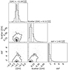 |
Fig. 6. Corner plot summary of the posterior distributions of the [Z/H], its scatter, and the degrees of freedom of the Student-t distribution obtained for the galaxies in the X-ray group environment bin. Contours are at the 68% and 95% probability levels. The 16%, 50%, and 84% intervals are indicated by dashed lines. |
4. Results and discussion
As described in the previous sections, we spectroscopically selected 74 massive quiescent galaxies in the COSMOS Wall volume, and we analysed their physical properties performing a joint fit of their spectra and photometric data.
We combined the results obtained on individual galaxies to characterise the galaxy properties for the entire sample and in the three different environments defined in Sect. 2. In the following we present the obtained results and compare them with other studies in literature (Sect. 4.1), and we finally discuss our results in the framework of the environmental effect on the evolution of the massive quiescent galaxies (Sect. 4.2).
4.1. Results and comparison with the literature
As described in Sect. 2, our selected sample of massive quiescent galaxies is representative of the entire population of galaxies in the stellar mass range of 10.47 < log M/M⊙ < 11.4. For each galaxy in the sample, we derived the following physical parameters: stellar mean metallicity, mean Agemodel, star formation timescale (τ), and dust extinction (AV). Using a Spearman rank correlation test, we found that none of these properties in each of the three environment bins are correlated with the stellar mass of the galaxies in each subsample with significance > 2σ. Therefore, the chosen small mass dynamic range and the uniformity of the mass distributions across the different environments enable the study of the environmental effects on galaxy properties. We then combined the physical properties of the individual galaxies using a hierarchical Bayesian approach to determine the parameters for the entire sample and the characterising the three environments of different galaxy densities.
Figure 7 shows the results obtained for Agemodel, [Z/H] and τ as a function of the environment. The shaded grey regions represent the intrinsic scatter of the individual measured parameters in each environment bin. It is interesting to note that all the fits have shown values of Agemodel/τ higher than 3, confirming the purity and the fast star formation of the selected quiescent sample. Regarding the AV parameter, we did not consider it as a quantity containing physical information, as it is has been derived from template fitting procedures and may partially account for potential mismatches between observations and models. At the same time, it is reassuring that we found a value of around 0.26 mag across all the environments (see Table 2) is consistent with results reported by other authors for massive galaxies at intermediate redshift (e.g. Citro et al. 2016).
From Table 2 and Fig. 7, a decreasing trend in the mass-weighted age of galaxies as a function of the environmental density is clearly evident. Galaxies in the X-ray groups have a typical mass-weighted mean age of 5.5 Gyr, and they become progressively younger moving towards less dense environments, with a typical age of 4 Gyr in the field, with a significance of almost 2σ. This means that galaxies in X-ray groups are about 1.5 Gyr older than those in the field, although the intrinsic scatter measured across all three environments exceeds 1.5 Gyr.
Median values of the marginalised posterior distribution of the agemodel, mass-weighted age, [Z/H], τ, and AV of the second level model.
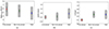 |
Fig. 7. Agemodel, [Z/H], and τ in different environments. Upper left panel: Median values of the agemodel with their relative error bars for different environments. Upper right panel: Median values of [Z/H] and their errors for different environments. Lower panel: Median values of τ and their errors for different environments. The grey shaded areas represent the intrinsic scatter of the individual posterior of the galaxies in each environment bin. |
The top-right panel of Fig. 7 shows that galaxies in the field exhibit a stellar metallicity value that is around 0.15 dex higher than those in denser environments, with a significance greater than 2σ. Galaxies in both X-ray and non-X-ray groups display similar metallicity values, around [Z/H] = −0.18 (i.e. 60% of the solar value).
Galaxies in X-ray groups appear quite homogeneous in their values of τ, representing the star formation timescale, and their measured τ value is significantly lower than those found in both the non-X-ray group environment and the field, even when accounting for the intrinsic scatter. It is worth noting that galaxies in non-X-ray groups and in the field present similar star formation timescales, but they differ by 0.6 Gyr in their mean mass-weighted age. The smaller intrinsic scatter observed in the stellar metallicity and τ for the sample in X-ray groups could indicate homogeneity in the physical processes that shaped these galaxies. In the next subsection we discuss possible explanations for this finding.
To check the robustness of our results, we compared them with those found by other authors in the literature. In particular, Darvish et al. (2017) proposed a different definition of the environment around the COSMOS Wall volume. In their work, they used the density field Hessian matrix to disentangle the cosmic web into clusters, filaments and field (see Darvish et al. 2016, 2017, for full details). The main difference between the Iovino et al. (2016) and the Darvish et al. (2017) definitions of environment is that the former applied a group detection algorithm and then checked for X-ray emitting or non-X-ray emitting ones, considering all other galaxies located in the field, while the latter locates the galaxies based solely on the density of the environment, considering a global smoothing width of 0.5 Mpc, thus somewhat larger than the typical virial radius of groups. Darvish et al. (2017) performed a less detailed analysis of the galaxy stellar population properties in different environments compared to the one presented here, and found that the intrinsic colours of massive quiescent galaxies do not depend on the environment. We considered the results obtained in our analysis while classifying galaxies following Darvish et al. (2017) criteria. Our results confirm the trend that galaxies in denser environments tend to be older, have lower stellar metallicities, and shorter formation timescales compared to those in the field.
We also compared our results with those of Sobral et al. (2022). Exploring the full LEGA-C sample at 0.6 < z < 1 and using the Darvish et al. (2017) definition of environment, they found that Dn4000 and Hδ indices for quiescent galaxies vary with both stellar mass and local density. In particular, at fixed stellar mass, their results suggest that quiescent galaxies residing in higher-density regions are older, meaning they formed the bulk of their stars earlier and quenched earlier. Their results are fully consistent with what we found in our analysis. Indeed, even in the narrow bin of mass and redshift we considered, we found that quiescent galaxies are older and with a shorter formation timescale in denser environment than in the field.
We compared our global results with those from other studies using LEGA-C data. Within the same redshift and mass range, the mass-weighted age of our sample (∼4.5 Gyr) is consistent within 0.5 Gyr with previous studies (e.g. Gallazzi et al. 2014; Chauke et al. 2018; Beverage et al. 2023; Kaushal et al. 2024), despite differences in stellar population models and analysis methodologies. It is also worth noting that the mean stellar metallicity of our sample (−0.1 dex) matches with the [Fe/H] abundance measured by Beverage et al. (2023). This further supports the robustness of our measurements, based solely on Fe indicators, suggesting that our total metallicity estimate effectively serves as a proxy for the [Fe/H] abundance.
In the local Universe, many previous studies have analysed the possible dependence of the physical properties of galaxies on the environment in which they are located. Sánchez-Blázquez et al. (2006) analysed quiescent galaxies in different environments, including Virgo and Coma clusters, finding that quiescent galaxies in lower-density environments appear younger by 1 − 2 Gyr that those in denser environments, at given galaxy stellar mass. Their results is consistent with what we found in this work at higher redshift, suggesting an almost passive evolution from z ∼ 0.7 to z = 0 for the most massive quiescent galaxies. A different conclusion is presented by Thomas et al. (2010). Using low-redshift data from the Sloan Digital Sky Survey (0.05 ≤ z ≤ 0.06), they found that the age and the stellar metallicity of the most massive quiescent galaxies do not depend on the environment and its density. Their results seem to suggest that the stellar population properties of the most massive quiescent galaxies are mainly driven by self-regulation processes related to intrinsic galaxy properties such as stellar mass. Our analysis of the properties of massive quiescent galaxies in the very narrow slice of redshift of the COSMOS Wall volume, at halfway of the Universe life, points out important differences related to the environment in which these galaxies are located. The differences we found are mainly in the mass-weighted age (i.e. galaxies in high-density environments are about 1.5 Gyr older than those in the field) and in the star formation timescale, which is roughly half in high-density environments compared to the field.
A possible explanation for the different results we found at z ∼ 0.7 compared to those reported in Thomas et al. (2010), could be related to the small age differences we detected between X-ray groups galaxies and field ones. Indeed, precise age estimation is much more challenging in the local Universe than at higher redshift, since the typical spectral indices sensitive to the age of the stellar content lose sensitivity for old ages. Age measurement errors of about 10% in the local Universe correspond to uncertainties of approximately 1 − 2 Gyr for ages around 10 Gyr. These uncertainties are of the same order as the age differences we estimated between galaxies in high- and low-density environments. Conversely, a limitation of our work is the relatively small sample size compared to those available at lower-z. Large surveys of quiescent galaxies at intermediate to high redshift will help reduce the statistical uncertainties affecting our work.
4.2. The environmental effect on stellar population parameters
The study of the age and the stellar metallicity provides valuable insights into the framework that describes the formation and the subsequent evolution of galaxies. In particular, thanks to the narrow redshift slice of the COSMOS Wall volume, the selection of a narrow stellar mass range, and detailed environment information from Iovino et al. (2016), we are able to investigate how the environment can affect the evolution of massive quiescent galaxies.
Figure 8 shows the cumulative mass fraction of the stellar mass as a function of the age of the Universe for galaxies in the three environments. As discussed in Sect. 4.1, X-ray group galaxies are older and exhibit a shorter star formation timescale with respect to the less dense environments (see also Fig. 7). This suggests that they began forming their stars earlier and quenched at an earlier stage. These findings support the idea that the SFH of massive quiescent galaxies in denser environments is regulated by additional mechanisms compared to those acting in the field. Such mechanisms are responsible for the removal of the cold gas in galaxies, causing a sudden and rapid quenching of star formation in contrast to the slower quenching observed in field galaxies. The observed dependence of the quenching timescale on environmental density, combined with the uniformity in stellar mass among the studied galaxies, suggests that mechanisms such as ram-pressure stripping, active predominantly in dense environments, play a key role in explaining the observed differences between galaxies in X-ray groups and those in the field. This result is in good agreement with the SFHs derived for massive elliptical galaxies by Guglielmo et al. (2015), where the analysed galaxies show a faster decline of their SFR in clusters compared to the field. Interestingly, Zhou et al. (2025) found a similar result, analysing the star-forming galaxies in the Wall volume. Their semi-analytical approach, applied to stacked spectra of star-forming galaxies in the Wall volume, grouped by bins of mass and environment, supports the view that galaxies in dense environments start their star formation earlier than field galaxies and have systematically shorter star formation timescales.
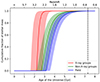 |
Fig. 8. Cumulative mass fraction of the stellar mass as a function of the age of the Universe obtained for the galaxies in the three environment bins. The solid lines mark the 50% percentile of the distributions, while contours are at the 16% and 84% confidence intervals. The vertical dashed line corresponds to the redshift of the COSMOS Wall structure (z ∼ 0.73). |
Regarding stellar metallicity, our analysis of massive quiescent galaxies shows that cluster galaxies have lower metallicity compared to those in the field. A lower stellar metallicity in high-density environments can be due to mechanisms such as ram-pressure stripping or tidal interactions, which remove gas reservoirs, curtail star formation, and limit the enrichment of the interstellar medium. Another possibility is that, in higher-density environments, the efficient dilution of metals in the cold gas reservoirs is driven by gas inflows from the lower metallicity intergalactic medium or by galaxy-galaxy interactions. In contrast, field galaxies benefit from prolonged gas availability, enabling extended star formation and chemical enrichment, which results in higher stellar metallicity. These results support the findings of Calabrò et al. (2022), who reported lower metallicities in galaxies in high-density environments compared to the field, even at higher redshifts. As mentioned above, it is important to note that, given the limited available wavelength range, we derived the total stellar metallicity in the sampled galaxies only on the basis of Fe indicators. In other words, the total metallicity we derived reflects the model assumption of the solar [Fe/Z] value. Massive quiescent galaxies, which formed very rapidly and early in the cosmic time, may be characterised by a [Fe/Z] < [Fe/Z]⊙ due to an enhanced abundance of α elements relative to Fe. Indeed, Borghi et al. (2022) and Bevacqua et al. (2023), analysing the LEGA-C spectra of quiescent galaxies found on average [α/Fe]> [α/Fe]⊙. Consequently, the trend in metallicity shown in Fig. 7 might reflect variations in [α/Fe] values across different environments, suggesting that the total metallicity could be higher than that measured. Notably, α-enhancement is expected in systems where stars formed on short timescales (Matteucci & Tornambe 1987; Thomas et al. 1999). Indeed, as reported in Table 2, we found that galaxies in X-ray groups are characterised by very short star formation timescales, shorter than those found in the other environments. This suggests that we may have underestimated the total metal content of galaxies in X-ray groups, which could be comparable to that of field galaxies, but with higher α-enhancement in X-ray groups galaxies than in the field ones. Again, this result well matches what Zhou et al. (2025) found for the most massive star-forming galaxies in the Wall volume and their gas-phase metallicity.
The obtained results offer the opportunity to distinguish different evolutionary paths and quenching processes of massive quiescent galaxies. X-ray groups are characterised by hotter and denser intra-cluster medium compared to that in the non-X-ray groups (e.g. Boselli & Gavazzi 2006; Tonnesen et al. 2007). As a result, galaxies in X-ray groups are likely to be more significantly impacted by ram-pressure stripping than those located in small and less dense groups. Conversely, galaxies in less massive groups have a higher probability of merging and/or interacting with one another due their lower relative velocities. Figure 7 shows that galaxies in non-X-ray groups exhibit younger ages than those in denser environment and older ages than those in the field. They have a stellar metallicity similar to that found in denser environment but a star formation timescale more akin to that of field galaxies. From Fig. 8 we can see that these galaxies started their star formation activity at a similar epoch as those in denser clusters, but quenched later due to less efficient quenching mechanisms. While our results suggest a non-negligible role of dynamical processes affecting the gas supply available to galaxies in X-ray groups, the earlier formation time could also imply that star formation occurred in different internal physical conditions, leading to a more efficient star formation activity (and thus an earlier exhaustion of gas supply) even in absence of an active role of the environment. In this respect, however, we can leverage the sample of the non-X-ray groups, in which galaxies formed earlier than in the field but with the same timescale, possibly due to a similar rate of galaxy interactions and mergers in these two environments.
Higher S/N data covering a larger wavelength range will provide a clearer picture of the evolution of massive quiescent galaxies. Indeed, measuring the [α/Fe] is essential for obtaining a reliable estimation of the total stellar metallicity of quiescent galaxies, enabling a deeper insight into their complex assembly history across different environments.
5. Summary and conclusions
We have presented an analysis of the stellar populations of a sample of 74 massive quiescent galaxies in the COSMOS Wall to investigate the role of the environment in galaxy evolution. The COSMOS Wall is a structure at z ∼ 0.73 that contains a large variety of environments, from rich and dense clusters down to empty field regions. The analysed sample was derived using the LEGA-C spectroscopic data; we selected galaxies with no detectable [OIII]λ5007 or Hβ emission lines and at most a weak [OII]λ3727 line. Additionally, we excluded post-starburst galaxies by requiring the Hδ absorption line with equivalent widths < 3 Å. From this sample, we selected galaxies in a narrow range of mass, 10.47 < log M/M⊙ < 11.4, in order to have a representative, homogeneous sample in the slice of redshift of the COSMOS Wall across the different environments. We used the environment characterisation from Iovino et al. (2016), from which we found 16 galaxies in groups with X-ray detection, 22 in groups without X-ray detection, and 36 in the field.
We combined the LEGA-C survey spectroscopic data, which have high S/N and resolution suitable for studying the stellar population properties of galaxies, with the multi-wavelength photometric COSMOS2020 catalogue. We performed a joint fitting of spectra and photometric data using nested sampling techniques in order to measure the mass-weighted age, stellar metallicity, and star formation timescale of individual galaxies. After that, we assessed the stellar population parameters of each environment bin using a hierarchical Bayesian approach. Our findings can be summarised as follows:
-
Quiescent galaxies in denser environments are about 1.5 Gyr older than those in the field.
-
There is no significant difference in stellar metallicity between galaxies in the X-ray and non-X-ray groups, both showing values of about 60% of the solar value. Field galaxies exhibit metallicities approximately 0.15 dex higher.
-
Galaxies in the X-ray groups have shorter star formation timescales. Those in the other two environment bins have similarly higher timescales despite a 1 Gyr difference in their mass-weighted ages.
Our results support the idea that the SFH of massive quiescent galaxies in denser environments is regulated by mechanisms different from those acting in the field. In particular, the presence of a hot and dense intra-cluster medium in the X-ray groups strongly suggests that ram-pressure stripping plays a key role in the quenching process. Processes like cosmological starvation could explain the physical parameters we observed in galaxies in the field, which have younger ages and longer star formation timescales compared to those in the X-ray groups. The longer star formation timescale of galaxies in non-X-ray groups indicates a more complex evolutionary history, likely driven by more frequent interactions and mergers, which is typical in less dense and smaller groups.
Upcoming surveys with new, high multiplexed, large field-of-view spectrographs, such as StePS at the WEAVE and 4MOST instruments (Iovino et al. 2023a,b), will provide the spectra of thousands of galaxies and cover wide spectral ranges with S/N suitable for measuring stellar population parameters. These data will allow us to measure the [α/Fe] of the stellar populations, which is crucial for obtaining a clearer picture of the star formation timescale of the massive quiescent galaxies and further understanding their complex assembly history across various environments.
Acknowledgments
We thank the anonymous referee for carefully reading the manuscript and for the stimulating suggestions that helped to improve the paper. S.Z., A.I., M.L., S.B., M.B., O.C., L.P., D.V., E.Z. and F.D. acknowledge financial support from INAF Large Grant 2022, FFO 1.05.01.86.16, and the Italian Ministry grant Premiale MITIC 2017. The authors wish to acknowledge the generous support of ESO staff during service observations of program ESO 085.A-0664 (The COSMOS Structure at z = 0.73: Exploring the Onset of Environment-Driven Trends), which provided the valuable environmental characterisation on which this work is based.
References
- Baldry, I. K., Balogh, M. L., Bower, R. G., et al. 2006, MNRAS, 373, 469 [Google Scholar]
- Balogh, M. L., Morris, S. L., Yee, H., Carlberg, R., & Ellingson, E. 1999, ApJ, 527, 54 [CrossRef] [Google Scholar]
- Balogh, M. L., Navarro, J. F., & Morris, S. L. 2000, ApJ, 540, 113 [Google Scholar]
- Bennett, C., Larson, D., Weiland, J., & Hinshaw, G. 2014, ApJ, 794, 135 [NASA ADS] [CrossRef] [Google Scholar]
- Bevacqua, D., Saracco, P., La Barbera, F., et al. 2023, MNRAS, 525, 4219 [NASA ADS] [CrossRef] [Google Scholar]
- Beverage, A. G., Kriek, M., Conroy, C., et al. 2023, ApJ, 948, 140 [NASA ADS] [CrossRef] [Google Scholar]
- Borghi, N., Moresco, M., Cimatti, A., et al. 2022, ApJ, 927, 164 [NASA ADS] [CrossRef] [Google Scholar]
- Boselli, A., & Gavazzi, G. 2006, PASP, 118, 517 [Google Scholar]
- Boselli, A., Fossati, M., & Sun, M. 2022, A&ARv, 30, 3 [NASA ADS] [CrossRef] [Google Scholar]
- Bruzual, G., & Charlot, S. 2003, MNRAS, 344, 1000 [NASA ADS] [CrossRef] [Google Scholar]
- Buchner, J. 2016, Stat. Comput., 26, 383 [Google Scholar]
- Buchner, J. 2019, PASP, 131, 108005 [Google Scholar]
- Buchner, J. 2021, J. Open Source Softw., 6, 3001 [CrossRef] [Google Scholar]
- Calabrò, A., Guaita, L., Pentericci, L., et al. 2022, A&A, 664, A75 [NASA ADS] [CrossRef] [EDP Sciences] [Google Scholar]
- Calzetti, D. 2001, PASP, 113, 1449 [Google Scholar]
- Cappellari, M. 2017, MNRAS, 466, 798 [Google Scholar]
- Cappellari, M. 2023, MNRAS, 526, 3273 [NASA ADS] [CrossRef] [Google Scholar]
- Cappellari, M., & Emsellem, E. 2004, PASP, 116, 138 [Google Scholar]
- Cassata, P., Guzzo, L., Franceschini, A., et al. 2007, ApJS, 172, 270 [Google Scholar]
- Chabrier, G. 2003, PASP, 115, 763 [Google Scholar]
- Chauke, P., van der Wel, A., Pacifici, C., et al. 2018, ApJ, 861, 13 [NASA ADS] [CrossRef] [Google Scholar]
- Chen, Y., Bressan, A., Girardi, L., et al. 2015, MNRAS, 452, 1068 [Google Scholar]
- Cicone, C., Maiolino, R., Sturm, E., et al. 2014, A&A, 562, A21 [NASA ADS] [CrossRef] [EDP Sciences] [Google Scholar]
- Citro, A., Pozzetti, L., Moresco, M., & Cimatti, A. 2016, A&A, 592, A19 [NASA ADS] [CrossRef] [EDP Sciences] [Google Scholar]
- Coil, A. L., Blanton, M. R., Burles, S. M., et al. 2011, ApJ, 741, 8 [Google Scholar]
- Comparat, J., Richard, J., Kneib, J.-P., et al. 2015, A&A, 575, A40 [NASA ADS] [CrossRef] [EDP Sciences] [Google Scholar]
- Cooper, M. C., Newman, J. A., Croton, D. J., et al. 2006, MNRAS, 370, 198 [CrossRef] [Google Scholar]
- Croton, D. J., Springel, V., White, S. D. M., et al. 2006, MNRAS, 365, 11 [Google Scholar]
- Cucciati, O., Iovino, A., Marinoni, C., et al. 2006, A&A, 458, 39 [NASA ADS] [CrossRef] [EDP Sciences] [Google Scholar]
- Darvish, B., Mobasher, B., Sobral, D., et al. 2016, ApJ, 825, 113 [NASA ADS] [CrossRef] [Google Scholar]
- Darvish, B., Mobasher, B., Martin, D. C., et al. 2017, ApJ, 837, 16 [Google Scholar]
- Davé, R., Finlator, K., & Oppenheimer, B. D. 2012, MNRAS, 421, 98 [Google Scholar]
- Davis, M., & Geller, M. J. 1976, ApJ, 208, 13 [NASA ADS] [CrossRef] [Google Scholar]
- Ditrani, F. R., Longhetti, M., Fossati, M., & Wolter, A. 2024, A&A, 688, A89 [NASA ADS] [CrossRef] [EDP Sciences] [Google Scholar]
- Dressler, A. 1980, ApJ, 236, 351 [Google Scholar]
- Fabian, A. C. 2012, ARA&A, 50, 455 [Google Scholar]
- Falcón-Barroso, J., Sánchez-Blázquez, P., Vazdekis, A., et al. 2011, A&A, 532, A95 [Google Scholar]
- Fossati, M., Wilman, D. J., Mendel, J. T., et al. 2017, ApJ, 835, 153 [Google Scholar]
- Gallazzi, A., Charlot, S., Brinchmann, J., White, S. D., & Tremonti, C. A. 2005, MNRAS, 362, 41 [NASA ADS] [CrossRef] [Google Scholar]
- Gallazzi, A., Bell, E. F., Zibetti, S., Brinchmann, J., & Kelson, D. D. 2014, ApJ, 788, 72 [Google Scholar]
- Gallazzi, A. R., Pasquali, A., Zibetti, S., & Barbera, F. L. 2021, MNRAS, 502, 4457 [NASA ADS] [CrossRef] [Google Scholar]
- George, M. R., Leauthaud, A., Bundy, K., et al. 2011, ApJ, 742, 125 [Google Scholar]
- Gozaliasl, G., Finoguenov, A., Tanaka, M., et al. 2019, MNRAS, 483, 3545 [Google Scholar]
- Gregg, M. D. 1994, ApJ, 108, 2164 [CrossRef] [Google Scholar]
- Guglielmo, V., Poggianti, B. M., Moretti, A., et al. 2015, MNRAS, 450, 2749 [NASA ADS] [CrossRef] [Google Scholar]
- Gunn, J. E., & Gott, J. R. 1972, ApJ, 176, 1 [NASA ADS] [CrossRef] [Google Scholar]
- Guzzo, L., Cassata, P., Finoguenov, A., et al. 2007, ApJS, 172, 254 [NASA ADS] [CrossRef] [Google Scholar]
- Iovino, A., Cucciati, O., Scodeggio, M., et al. 2010, A&A, 509, A40 [NASA ADS] [CrossRef] [EDP Sciences] [Google Scholar]
- Iovino, A., Petropoulou, V., Scodeggio, M., et al. 2016, A&A, 592, A78 [NASA ADS] [CrossRef] [EDP Sciences] [Google Scholar]
- Iovino, A., Poggianti, B. M., Mercurio, A., et al. 2023a, A&A, 672, A87 [NASA ADS] [CrossRef] [EDP Sciences] [Google Scholar]
- Iovino, A., Mercurio, A., Gallazzi, A. R., et al. 2023b, The Messenger, 190, 22 [NASA ADS] [Google Scholar]
- Kaushal, Y., Nersesian, A., Bezanson, R., et al. 2024, ApJ, 961, 118 [NASA ADS] [CrossRef] [Google Scholar]
- Larson, R. B., Tinsley, B. M., & Caldwell, C. N. 1980, ApJ, 237, 692 [Google Scholar]
- Lilly, S. J., Le Fèvre, O., Renzini, A., et al. 2007, ApJS, 172, 70 [Google Scholar]
- Man, A., & Belli, S. 2018, Nat. Astron., 2, 695 [NASA ADS] [CrossRef] [Google Scholar]
- Marigo, P., Bressan, A., Nanni, A., Girardi, L., & Pumo, M. L. 2013, MNRAS, 434, 488 [Google Scholar]
- Martín-Navarro, I., Pérez-González, P. G., Trujillo, I., et al. 2014, ApJ, 798, L4 [CrossRef] [Google Scholar]
- Martín-Navarro, I., Lyubenova, M., van de Ven, G., et al. 2019, A&A, 626, A124 [Google Scholar]
- Maseda, M. V., van der Wel, A., Franx, M., et al. 2021, ApJ, 923, 18 [NASA ADS] [CrossRef] [Google Scholar]
- Matteucci, F., & Tornambe, A. 1987, A&A, 185, 51 [Google Scholar]
- Mihos, J. C., & Hernquist, L. 1996, ApJ, 464, 641 [Google Scholar]
- Moore, B., Lake, G., & Katz, N. 1998, ApJ, 495, 139 [Google Scholar]
- Muzzin, A., Marchesini, D., Stefanon, M., et al. 2013, ApJ, 777, 18 [NASA ADS] [CrossRef] [Google Scholar]
- Oemler, A. 1974, ApJ, 194, 1 [Google Scholar]
- Oke, J. B. 1974, ApJS, 27, 21 [Google Scholar]
- Peng, Y.-J., Lilly, S. J., Kovač, K., et al. 2010, ApJ, 721, 193 [Google Scholar]
- Pietrinferni, A., Cassisi, S., Salaris, M., & Castelli, F. 2004, ApJ, 612, 168 [Google Scholar]
- Pietrinferni, A., Cassisi, S., Salaris, M., & Castelli, F. 2006, ApJ, 642, 797 [Google Scholar]
- Plat, A., Charlot, S., Bruzual, G., et al. 2019, MNRAS, 490, 978 [Google Scholar]
- Poggianti, B. M., von der Linden, A., De Lucia, G., et al. 2006, ApJ, 642, 188 [NASA ADS] [CrossRef] [Google Scholar]
- Poggianti, B. M., Aragón-Salamanca, A., Zaritsky, D., et al. 2009, ApJ, 693, 112 [NASA ADS] [CrossRef] [Google Scholar]
- Poggianti, B. M., Calvi, R., Bindoni, D., et al. 2013, ApJ, 762, 77 [NASA ADS] [CrossRef] [Google Scholar]
- Sánchez, S., Barrera-Ballesteros, J., Lacerda, E., et al. 2022, ApJS, 262, 36 [CrossRef] [Google Scholar]
- Sánchez-Blázquez, P., Peletier, R., Jiménez-Vicente, J., et al. 2006, MNRAS, 371, 703 [CrossRef] [Google Scholar]
- Scoville, N., Aussel, H., Brusa, M., et al. 2007a, ApJS, 172, 1 [Google Scholar]
- Scoville, N., Aussel, H., Benson, A., et al. 2007b, ApJS, 172, 150 [Google Scholar]
- Sobral, D., van der Wel, A., Bezanson, R., et al. 2022, ApJ, 926, 117 [NASA ADS] [CrossRef] [Google Scholar]
- Spitzer, L., & Baade, W. 1951, ApJ, 113, 413 [NASA ADS] [CrossRef] [Google Scholar]
- Straatman, C. M., van der Wel, A., Bezanson, R., et al. 2018, ApJS, 239, 27 [NASA ADS] [CrossRef] [Google Scholar]
- Thomas, D., Greggio, L., & Bender, R. 1999, MNRAS, 302, 537 [NASA ADS] [CrossRef] [Google Scholar]
- Thomas, D., Maraston, C., Bender, R., & De Oliveira, C. M. 2005, ApJ, 621, 673 [NASA ADS] [CrossRef] [Google Scholar]
- Thomas, D., Maraston, C., Schawinski, K., Sarzi, M., & Silk, J. 2010, MNRAS, 404, 1775 [NASA ADS] [Google Scholar]
- Tonnesen, S., Bryan, G. L., & van Gorkom, J. H. 2007, ApJ, 671, 1434 [Google Scholar]
- van der Wel, A., Noeske, K., Bezanson, R., et al. 2016, ApJS, 223, 29 [Google Scholar]
- van der Wel, A., Bezanson, R., D’Eugenio, F., et al. 2021, ApJS, 256, 44 [NASA ADS] [CrossRef] [Google Scholar]
- Vazdekis, A., Koleva, M., Ricciardelli, E., Röck, B., & Falcón-Barroso, J. 2016, MNRAS, 463, 3409 [Google Scholar]
- Weaver, J. R., Kauffmann, O. B., Ilbert, O., et al. 2022, ApJS, 258, 11 [NASA ADS] [CrossRef] [Google Scholar]
- Whitaker, K. E., van Dokkum, P. G., Brammer, G., et al. 2013, ApJ, 770, L39 [NASA ADS] [CrossRef] [Google Scholar]
- Williams, R. J., Quadri, R. F., Franx, M., van Dokkum, P., & Labbé, I. 2009, ApJ, 691, 1879 [NASA ADS] [CrossRef] [Google Scholar]
- Worthey, G., Faber, S., Gonzalez, J. J., & Burstein, D. 1994, ApJS, 94, 687 [NASA ADS] [CrossRef] [Google Scholar]
- Zhou, S., Iovino, A., Longhetti, M., et al. 2025, A&A, in press, https://doi.org/10.1051/0004-6361/202452889 [Google Scholar]
All Tables
The seven free parameters fitted to our spectroscopic and photometric data, along with their associated prior distributions.
Median values of the marginalised posterior distribution of the agemodel, mass-weighted age, [Z/H], τ, and AV of the second level model.
All Figures
|
Fig. 1. Rest-frame UVJ diagram of the selected sample. The stars are all the galaxies observed in the COSMOS Wall volume by the LEGA-C survey, while the red points mark the spectroscopically selected quiescent galaxies. The solid black line is the separation between star-forming and quiescent galaxies as defined in Eq. (4) of Williams et al. (2009). The dotted line divides younger quiescent galaxies (on the left) and older quiescent galaxies (on the right) according to Whitaker et al. (2013). |
| In the text | |
|
Fig. 2. Mass distribution in the three environment bins. The shaded grey region is the mass cut we applied to obtain a homogeneous and representative distribution across the three bins. |
| In the text | |
|
Fig. 3. FIF application to the indices available in the LEGA-C ID 209466 galaxy spectrum. The vertical dashed brown lines indicate the feature boundaries for each index, while the grey shaded regions represent the pseudo-continua used for normalisation. In the upper subplots, the black lines and blue shaded regions correspond to the observed spectrum and its associated uncertainty, respectively. The solid red line represents the best-fit derived from the posterior distribution. The green lines in the lower subplots show the residuals between the observed spectrum and the best fit, with the yellow shaded region indicating the relative uncertainties of the observed spectrum. |
| In the text | |
|
Fig. 4. Example of the joint and marginal posterior distributions for the LEGA-C ID 209466 galaxy. Contours represent the 68% and 95% probability levels. The 16%, 50%, and 84% intervals are indicated as dashed lines. |
| In the text | |
|
Fig. 5. Panel (a), top: Example of the best fit (in red) applied to the entire LEGA-C spectrum of the LEGA-C ID 209466 galaxy (in black). Panel (a), bottom: Difference between the observed spectrum and the best fit, shown in green, and the relative uncertainties of the observed spectrum, shown in yellow. Panel (b): Observed photometric measurements (blue points), best-fitting template (in red), and photometric measurements on the best-fitting template (lime stars). The green shaded region indicates the 68% confidence interval of our posterior. |
| In the text | |
|
Fig. 6. Corner plot summary of the posterior distributions of the [Z/H], its scatter, and the degrees of freedom of the Student-t distribution obtained for the galaxies in the X-ray group environment bin. Contours are at the 68% and 95% probability levels. The 16%, 50%, and 84% intervals are indicated by dashed lines. |
| In the text | |
|
Fig. 7. Agemodel, [Z/H], and τ in different environments. Upper left panel: Median values of the agemodel with their relative error bars for different environments. Upper right panel: Median values of [Z/H] and their errors for different environments. Lower panel: Median values of τ and their errors for different environments. The grey shaded areas represent the intrinsic scatter of the individual posterior of the galaxies in each environment bin. |
| In the text | |
|
Fig. 8. Cumulative mass fraction of the stellar mass as a function of the age of the Universe obtained for the galaxies in the three environment bins. The solid lines mark the 50% percentile of the distributions, while contours are at the 16% and 84% confidence intervals. The vertical dashed line corresponds to the redshift of the COSMOS Wall structure (z ∼ 0.73). |
| In the text | |
Current usage metrics show cumulative count of Article Views (full-text article views including HTML views, PDF and ePub downloads, according to the available data) and Abstracts Views on Vision4Press platform.
Data correspond to usage on the plateform after 2015. The current usage metrics is available 48-96 hours after online publication and is updated daily on week days.
Initial download of the metrics may take a while.