| Issue |
A&A
Volume 632, December 2019
|
|
|---|---|---|
| Article Number | A99 | |
| Number of page(s) | 14 | |
| Section | Galactic structure, stellar clusters and populations | |
| DOI | https://doi.org/10.1051/0004-6361/201936196 | |
| Published online | 10 December 2019 | |
Axisymmetric Schwarzschild models of an isothermal axisymmetric mock dwarf spheroidal galaxy
Kapteyn Astronomical Institute, University of Groningen, PO Box 800 9700 AV Groningen, The Netherlands
e-mail: This email address is being protected from spambots. You need JavaScript enabled to view it.
Received:
27
June
2019
Accepted:
7
October
2019
Abstract
Aims. The goal of this work is to test the ability of Schwarzschild’s orbit superposition method to measure the mass content, scale radius, and shape of a flattened dwarf spheroidal galaxy. Until now, most dynamical model efforts have assumed that dwarf spheroidal galaxies and their host halos are spherical.
Methods. We used an Evans model (1993, MNRAS, 260, 191) to construct an isothermal mock galaxy whose properties somewhat resemble those of the Sculptor dwarf spheroidal galaxy. This mock galaxy contains flattened luminous and dark matter components, resulting in a logarithmic profile for the global potential. We tested whether the Schwarzschild method could constrain the characteristic parameters of the system for different sample sizes and whether this was possible without knowledge of the functional form of the potential.
Results. When assuming the true functional form of the potential of the system, the Schwarzschild modelling technique is able to provide an accurate and precise measurement of the characteristic mass parameter of the system and accurately reproduces the light distribution and the stellar kinematics of our mock galaxy. When assuming a different functional form for the potential of the model, such as a flattened Navarro–Frenk–White (NFW) profile, we also constrain the mass and scale radius to their corresponding values. However in both cases, we find that the flattening parameter remains largely unconstrained. This is likely because the information content of the velocity dispersion on the geometric shape of the potential is too small.
Conclusions. Our results using Schwarzschild’s method indicate that the mass enclosed can be derived reliably, even if the flattening parameter is unknown, and already for samples containing 2000 line-of-sight radial velocities, such as those currently available. Further applications of the method to more general distribution functions of flattened systems are needed to establish how well the flattening of dSph dark halos can be determined.
Key words: dark matter / galaxies: dwarf / galaxies: kinematics and dynamics
© ESO 2019
1. Introduction
In the current cosmological ΛCDM model most of the mass is believed to be in the form of (cold) dark matter. While successful on large scales, on the scales of dwarf galaxies, the model suffers a number of challenges, including the missing satellites problem (Klypin et al. 1999; Moore et al. 1999), the cusp-core conundrum (Hui 2001), and the too-big-to-fail problem (Boylan-Kolchin et al. 2011), although all may be solved one way or another by considering the effects of baryonic physics (e.g. Zolotov et al. 2012; Brooks et al. 2013; Wetzel et al. 2016; Kim et al. 2018). The dwarf spheroidal satellite galaxies (dSphs or dSph galaxies) of our Milky Way can provide particularly strong constraints on the nature of dark matter, since their high mass-to-light ratios suggest that they are fully dark-matter dominated (Strigari et al. 2008; Walker et al. 2007; Wolf et al. 2010).
Various methods have been used to develop dynamical models of dSph galaxies using line-of-sight velocity measurements for large samples of individual stars in these systems (e.g. Battaglia et al. 2006, 2008a,b, 2011; Walker et al. 2009a, 2015). Modelling via the Jeans Equations, distribution functions, and orbit superposition methods like Schwarzschild modelling are amongst those most often used (Battaglia et al. 2013). All these methods have in common that they assume that the systems are in dynamical equilibrium.
The Jeans Equations are derived by taking moments of the Collisionless Boltzmann Equation, which itself describes the conservation of probability in phase-space (Binney & Tremaine 2008). Not every solution of the Jeans Equations has an associated distribution function that is physical (i.e. positive) everywhere. Furthermore, finding a solution requires additional assumptions, for example on the functional form of the density profile and on the velocity anisotropy (because this is generally not known, although see the work by Massari et al. 2018, who determined directly the anisotropy of a sample of stars in the Sculptor dSph using proper motions derived from Gaia and HST). Because Jeans modelling is very flexible and fast, it has become the most widely used tool to model dSph galaxies, particularly in the spherical limit. It has, for example, allowed a robust (independent of the velocity anisotropy) measurement of the mass enclosed within approximately the half light radius of the dSph galaxies (Walker et al. 2009b; Wolf et al. 2010), and the determination that the masses of the classical dSphs are in the range ∼(108 − 109) M⊙ (e.g. Walker et al. 2007). On the other hand, it has not been possible to rule out cusped or cored profiles on the basis of these types of models (e.g. Evans et al. 2009; Strigari et al. 2017).
The Schwarzschild (1979) modelling technique relies on the idea that a system can be seen as a superposition of stellar orbits. In Schwarzschild modelling, one only needs to assume a specific gravitational potential form. The method does require a significant amount of computing power and therefore a smaller set of gravitational potentials can be explored in comparison to Jeans modelling. Breddels & Helmi (2013) applied this method to four dwarf spheroidal galaxies, and by modelling both the second and fourth line-of-sight velocity moments and assuming spherical symmetry they find that, independently of the particular form assumed for the potential, it is possible to constrain not only the mass at around the half-light radius (more precisely at r−3 where the logarithmic slope of the luminous density is −3) but also the logarithmic slope of the dark matter density.
Most work thus far has assumed that dwarf spheroidal galaxies and their host halos are spherical, despite the fact that their light distribution is typically not spherical (Irwin & Hatzidimitriou 1995; McConnachie 2012). Furthermore, dark matter halos are predicted to be triaxial (Jing & Suto 2002) when no baryonic effects are taken into account, although subhalos in cold dark matter simulations that could host dSphs are only mildly triaxial, and almost axisymmetric (Vera-Ciro et al. 2014). This implies that it is important to establish how many and which of the previously mentioned results still stand when taking into account deviations from spherical symmetry.
Kowalczyk et al. (2017, 2018) studied the ability of recovering the mass profile and anisotropy of the remnants of the mergers of dwarf disky galaxies (one postulated channel for the formation of dSphs) when using spherical Schwarzschild models. These latter authors showed that for spherical remnants the method can break the mass–anisotropy degeneracy, whereas for non-spherical (prolate) remnants the anisotropy will always be underestimated, although the total mass profile will be recovered well for data along the minor axis (although not if the data are along the major axis).
On the other hand, Hayashi & Chiba (2012, 2015) used axisymmetric Jeans modelling to infer the axis ratio of the dark matter density distribution (Q) in several dSphs assuming a constant velocity anisotropy βz. These latter authors report rather low axis ratios (Q = [0.3 − 0.5]) compared to the observed projected axial ratio in the light ( ). These low values are somewhat counterintuitive, though the results may be affected by degeneracies between Q, the velocity anisotropy profile, the viewing angle of the dSph, and the inner slope of the dark matter density profile. In Hayashi et al. (2016), a very similar technique was applied to unbinned data, and for the Sculptor dSph for example, the authors found that the flattening parameter is largely unconstrained.
In this work we explore the performance of the Schwarzschild modelling technique in the axisymmetric regime to free ourselves from the assumptions inherent to Jeans models. We test the method on a mock Sculptor-like dSph and consider axisymmetric mass distributions for both the light and the dark matter component and establish how well the characteristic parameters of the potential can be recovered for different sample sizes.
The paper is organised as follows. In Sect. 2, we set up a mock galaxy and simulate a realistic dataset. In Sect. 3 we describe the Schwarzschild method and its implementation in this work. In Sect. 4.1, we then apply the Schwarzschild method and show that we can recover the characteristic mass parameter of the mock galaxy potential, irrespective of the potential flattening parameter assumed. In Sect. 4.2 we model our mock galaxy with an axisymmetric NFW potential form and show that, even in this case, the Schwarzschild method is able to constrain the mass and scale radius to the corresponding values for datasets containing a realistic number of stars. We present our conclusions in Sect. 5 where we also discuss our findings.
2. The mock galaxy
2.1. Potential, luminous density, and characteristic parameters
We have built a mock galaxy inspired by the Sculptor dSph. We assume a flattened stellar density profile (q* = 0.8), no net rotation, and a line-of-sight velocity dispersion of ∼10 km s−1 (Mateo 1998; Battaglia et al. 2008a; Walker et al. 2009b). For simplicity, we have set up the mock galaxy following Evans (1993), who uses an elementary distribution function to describe a composite axisymmetric system. This distribution function is ergodic, meaning that it leads to a velocity ellipsoid that is isotropic and has a constant amplitude and thus is not generic1. Even though the velocity anisotropies of most classical dSphs do not appear to be too far from isotropic (see e.g. Hayashi & Chiba 2015; Hayashi et al. 2016; Hayashi & Obata 2019; Massari et al. 2019, but also Massari et al. 2018), our specific choice of an isotropic model might be a simplification of reality.
The gravitational potential of the composite system as a whole follows the form
 (1)
(1)
where (R, ϕ, z) denote the cylindrical coordinates. Here,  relates to the mass of the system and Rc is the core radius. The parameter q is the axial ratio of the potential, and has to satisfy
  where the lower limit is set by the condition that the spatial density is positive everywhere (Binney & Tremaine 2008) and the upper limit yields a composite distribution function of the form used by Evans (1993) that is positive everywhere. The zero point of the potential is set by Φ0.
The density profile of the stellar component is described by
 (2)
(2)
where ρ0 is the central density, p denotes a slope parameter, and q* is the axial ratio of the stellar density. The associated stellar distribution function is given by
![Mathematical equation: $$ \begin{aligned} f_{\text{ lum}}(E) \propto \text{ exp}[-pE/v_0^2] = \text{ exp}[-p\Phi _\text{ E}/v_0^2] \,\, \text{ exp}[-pv^2/2v_0^2], \end{aligned} $$](/articles/aa/full_html/2019/12/aa36196-19/aa36196-19-eq6.gif) (3)
(3)
where E is the sum of the gravitational potential and kinetic energies of a star.
Throughout the paper we define the flattening of a system as the axial ratio of the equipotential contours. In the Evans model, q* = q and therefore the axial ratio of the stellar density component is the same as that of the potential (not the density) of the composite system. For q < 1, the system is said to be oblate, and prolate for q > 1. The surface brightness profile of the mock galaxy can be found by integrating the luminous density along the line-of-sight.
The line-of-sight velocity profile is exactly Gaussian with a velocity dispersion that is isotropic and constant everywhere:
 (4)
(4)
and independent of the inclination, scale radius, and flattening parameter.
We choose here v0 = 20 km s−1, Rc = 1 kpc, q = 0.8, and p = 3.5 for our mock galaxy. These values result in a velocity dispersion of roughly 10.7 km s−1. For these values of p and q, the central total density should be at least 1.13 times the central stellar density to yield positive phase-space densities for both the stellar and dark components everywhere.
2.2. Observing the mock galaxy
We place the mock galaxy at a distance of 80 kpc, and “observe” it with a square field of view (FOV), centred on the mock galaxy, with a size of 7832″ × 7832″ (which then corresponds to roughly 3 × 3 kpc)2. The sky coordinates therefore range from roughly −1.5 kpc to +1.5 kpc. Throughout this work we assume an edge-on view.
In Fig. 1 we show the resulting 2D surface brightness profile of the mock galaxy for an edge-on view and as a function of the sky coordinates x′ and y′. Since the galaxy is axisymmetric, we only show the positive quadrant. Contours of constant surface brightness follow ellipses with axial ratios  , which because of the edge-on view are identical to those of the intrinsic density (i.e.
  ). The 1D surface brightness profile along the major axis is plotted in the top panel of this figure. The surface brightness decreases by a factor of two with respect to its central value at a projected ellipsoidal radius of 0.86 kpc, however the projected half light radius is much larger (3.87 kpc).
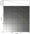 |
Fig. 1. Surface brightness profile of our mock galaxy in an edge-on view. The black horizontal and vertical lines show the boundaries of the kinematic bins. We only show the positive quadrant of our FOV (x′> 0 kpc, y′> 0 kpc). The yellow contours correspond to the isophotes of the system (q* = q = 0.8). In the top panel we have plotted the surface brightness normalised to its central value as function of x′, i.e. along the (projected) major axis of the galaxy. |
We generate kinematic data for the mock galaxy by drawing positions of stars following the luminous density distribution (see Eq. (2)) and velocities from the Gaussian distribution function (see Eq. (3)). We thus assume that the dataset of the stars with measured line-of-sight velocities follows the same distribution as the light.
The typical line-of-sight velocity measurements of individual stars have errors of order dv = 2 km s−1 (Battaglia et al. 2008b; Walker et al. 2009a). Therefore, to simulate a realistic kinematic dataset we convolve the line-of-sight velocities with a Gaussian distribution having a standard deviation of 2 km s−1. We compute velocity moments by combining the velocities of all available stars in a certain spatial bin on the sky (in what follows a kinematic bin) in our FOV. This binning is thus performed in the projected sky coordinates x′ and y′. The black horizontal and vertical lines visible in Fig. 1 show the borders of the kinematic bins from the positive quadrant. The velocity moments are estimated by correcting for the measurement errors (see Appendix A), similarly to Breddels et al. (2013). We assume that the surface brightness profile can be measured without error in much smaller spatial bins on the sky (which we refer to as light bins). To produce a reasonable galaxy, we also assume that the 3D light distribution is known to much larger radii, but for many fewer bins (more details can be found in Sect. 3.1).
3. The Schwarzschild orbit superposition method
In Schwarzschild modelling, orbits are used as building blocks of a dynamical system. Given a potential Φ, a complete set of orbits are integrated numerically and for each orbit the predicted observables are stored in a so-called orbit library. Varying the parameters of the potential (or varying the potential form as a whole), results in different libraries. The library that provides a combination of weighted orbits that best matches the observations (light profile + kinematics) is said to yield the best-fit parameters of the potential. The orbital weights themselves provide the corresponding distribution function. Since the orbital weights are positive by construction, the distribution function is non-negative everywhere.
3.1. Generating orbit libraries
In this paper we use a slightly modified version of the Schwarzschild code from van den Bosch et al. (2008), who modelled the elliptical galaxy NGC 4365. In what follows, we briefly describe how we generated the orbit libraries, how the orbital integration has been done, and how the libraries are stored. For more information we refer the reader to van den Bosch et al. (2008)3.
Given an energy Ei, initial positions x0 and z0 are sampled on an open polar grid, which is defined by NI2 polar angles and NI3 radii in between a thin orbit and the equipotential. The polar angles are sampled linearly, but to obtain a better sampling of orbits near the major axis of the system, 50% of the polar angles are sampled from the z-axis towards 10° above the midplane, and the remaining 50% from 10° down to the z = 0 plane. The initial y-coordinates and initial velocities in the x- and z-directions are set to zero. The initial velocities in the y-direction, vy, 0, are determined by  . This is done for all Nener energies, which are defined by Ei = Φ(x = xi, y = 0, z = 0). The locations xi that fix the energy grid are logarithmically sampled between 25 pc and 50 kpc from the centre. Such sampling also makes it possible to model a reasonable light distribution at distances well outside our FOV (more detailed information about the 3D grid used for this purpose is given below). This “orbit library” therefore consists of Norb = Nener × NI2 × NI3 orbits (z-tubes in our axisymmetric potential).
To account for slowly precessing orbits in the library we also compute 17 copies of each orbit, where each copied orbit is subsequently rotated by 10° in the xy-plane. These 18 copies are summed into a single orbit and replace the non-rotated orbit, such that each orbit now follows the axisymmetric requirements. Besides ensuring the axisymmetric behaviour of our models, adding rotations also increases the sampling of an orbit. We also note that each orbit has a counter-rotating sibling, obtained by appropriately changing the sign of the velocity vector.
We further improve the accuracy of the model by “dithering”: every orbit is split into  suborbits by replacing each of its three nonzero initial coordinates by Ndither slightly different coordinates. The initial conditions of all suborbits are found by increasing Nener, NI2, and NI3 by a factor of Ndither. The observables of each set of adjacent
  suborbits are combined and stored as being the observables of the (bundled) orbit. Choosing an odd number for Ndither ensures that the original orbit is the central suborbit of the bundle. In all our Schwarzschild models we use Ndither = 5. Every main orbit is thus made from a bundle of 53 = 125 neighbouring suborbits.
We use a Runge Kutta integrator to compute the stellar trajectories over roughly 200 orbital timescales. We require that the energy of each suborbit is always conserved better than 1% by increasing the accuracy of the integrator if necessary. For each orbit the kinematic information is stored in a velocity grid, which consists of a line-of-sight velocity axis (Nv velocity bins) and an axis associated to the location on the sky (Nkin kinematic bins). On equally spaced time intervals, a count is added to the element of the grid associated to the velocity and location at the given time. The sky projected path of the orbit is determined in a similar way and stored in the surface brightness grid containing N2D light light bins. In an additional 3D grid containing N3D light = 800 bins (40 radial, 5 azimuthal, and 4 polar bins in the positive octant) the 3D path of an orbit is stored. This 3D grid contains the same radii as used to sample the energies for the initial conditions and thus reaches well beyond the FOV (in contrast to the velocity and surface brightness grid). It is used to match the (3D) light distribution of the system at such radii.
In this work we set N2D light equal to 99 × 99 = 9801 and Nkin to 9 × 9 = 81, unless stated otherwise. The velocity axis of the velocity grid contains Nv = 41 bins and has a total velocity width of 80 km s−1, such that we cover velocities up to ±4σE. The central velocity bin is centred on 0 km s−1. To be able to track how long an orbit spends in a given kinematic bin, we need to account for the time spent with velocities outside the velocity grid (at that position). Therefore counts are also added to the first or last velocity bin if velocities are beyond the limits of the velocity grid.
When taking too few (i.e. too wide) velocity bins for the velocity grid, the velocity moments might not be recovered correctly. We checked that if we bin the theoretical Gaussian line-of-sight velocity profile of our mock galaxy as described above, thus discarding the contribution of velocities that are outside the range of the grid, the velocity moments are recovered well, that is the first and third moments are not affected, while the second and fourth velocity moments might result in relative errors of order 0.1% and 2% given the choices made for binning the velocity data.
3.2. Fitting orbital weights
Once the orbit libraries are in place, we find the orbital weights such that the total luminous mass, the surface brightness profile and the kinematics within the FOV, and the 3D light profile of the system are reproduced.
The 2D light profile is fitted using the surface brightness grid, where we define:
 (5)
(5)
where we sum over all orbits i. Here,  is the fraction of time orbit i spent in light bin j and
  is the fractional surface brightness in light bin j. The orbital weights are denoted by wi and add to unity by construction. The 3D light profile is fitted similarly using the 3D grid.
At the same time as we fit the light, we also fit the kinematics. In every kinematic bin k we compute the first four mass-weighted velocity moments  by defining:
 (6)
(6)
where again we sum over all orbits i. This time  is the fraction of time orbit i spent in kinematic bin k and
  is the fractional surface brightness in kinematic bin k. The nth moment of orbit i in kinematic bin k is given by
  :
:
 (7)
(7)
where △v is the size of the velocity bin and hikl is the fraction of time that orbit i spent in kinematic bin k and velocity bin l. Velocity bin l has velocity range [ ,
,  ], where vcen, l denotes its central velocity. We sum over the Nv velocity bins, although we discard the contributions of the first and last velocity bin. This is done since we did not set a stringent outer velocity boundary in these velocity bins: as described before, counts will be added here even if a star has a velocity outside the range of the grid and therefore the typical velocities of these bins are not known. We note that
  with this choice.
Now that we have defined the relation between the observables and the quantities in our model, we can describe how we fit the orbital weights. The fit is based on minimising  :
:
![Mathematical equation: $$ \begin{aligned} \chi ^2_{\text{ tot}} = \sum \limits ^{N_\text{ obs}}_{u=1} \left[ \frac{\text{ Model}\,[u] - \text{ Data}\,[u]}{\text{ Error}\,[u]} \right]^2, \end{aligned} $$](/articles/aa/full_html/2019/12/aa36196-19/aa36196-19-eq26.gif) (8)
(8)
where u runs over all Nobs observables. The number of observables is given by:
 (9)
(9)
which includes the contribution of the total light of the system, the fractional light for each 2D and 3D light bin, and the four velocity moments for each kinematic bin, respectively. We choose to use four velocity moments, since using higher-order moments might reduce the degeneracy between the velocity anisotropy and the mass profile (e.g. Merrifield & Kent 1990; Richardson & Fairbairn 2013). We do not use higher moments since these are observationally harder to constrain. The odd velocity moments are used to ensure that the Schwarzschild model also matches the observed mean rotation and the skewness of velocity distribution.
We use a non-negative least-squares solver to ensure that all orbital weights are positive. The light is weighted by assigning an error of 2% to each of the 2D and 3D light bins. We note that we can investigate the individual contribution to the total  by decomposing it; for example,
 (10)
(10)
We stress that  is being minimised. We do not minimise the terms on the right-hand side individually. The term associated to the total light of the system turns out to be negligible, since it is always recovered very well. The same holds for
  . These terms are only added to Eq. (8) to ensure that the model returns a realistic galaxy (in the sense that the luminous component might resemble a galaxy). Most of the constraining power therefore comes from the surface brightness profile and the kinematics.
4. Results
In this section we show that the Schwarzschild method can recover some of the characteristic parameters of the mock Sculptor-like dwarf spheroidal galaxy. We first show in Sect. 4.1 that if the true functional form of the potential of the system is known, we can constrain the characteristic mass parameter of the mock galaxy. In reality however, the true functional form of the potential of the system is not known. Therefore, in Sect. 4.2 we demonstrate how well we can constrain characteristic parameters when assuming an axisymmetric form of a Navarro–Frenk–White (NFW, Navarro et al. 1996) potential.
4.1. Two parameter Evans models: recovering the mock galaxy parameters
Here we assume the true functional form of the potential of the system is known, and we use it to build the orbit libraries for the Schwarzschild models. Our aim is to establish whether we can recover the correct values of the characteristic input parameters with this method. To this end we make a grid of models in which we vary the values of the characteristic parameters q and v0 (see Eq. (1)). We fix the core radius to Rc = 1 kpc, that is, to its true value. We sample q from 0.72 to 0.96, and v0 from 11 km s−1 to 29 km s−1, with higher sampling (decided iteratively) with steps in q of 0.02 and in v0 of 1 km s−1. We name the models by the values of their parameters: qXXvYY in which XX = 100q and YY = v0 in km s−1. For the orbit sampling, we set Nener = 32, NI2 = 32 and NI3 = 16 such that a total of 32 × 32 × 16 × 53 = 2 048 000 suborbits are integrated (see Sect. 3.1) and 2 × 32 × 32 × 16 = 32 768 orbital weights are determined (see Sect. 3.2).
4.1.1. Results for a large sample
We start with an idealised case in which the kinematic data consist of 105 stars. For 9 × 9 kinematic-bins on the sky, the typical error of the velocity dispersion in a kinematic bin is ∼0.25 km s−1.
The large panel of Fig. 2 shows the results obtained by fitting the Schwarzschild models to the data. The small black circles show the grid of tested values for q and v0, the green circle the true input values, and the white cross indicates the values of the parameters corresponding to the maximum likelihood estimator (MLE). For the best-fit model q94v21 we find  . The contribution of the kinematics (see Eq. (8)) to this value is 205.6. Using 81 kinematic bins to fit four velocity moments, this corresponds to 0.64 per kinematic constraint.
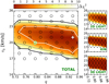 |
Fig. 2. Δχ2-distribution of the characteristic parameters q and v0 of the Evans models obtained after applying the Schwarzschild method. In this case our mock kinematic data consist of 105 stars inside the FOV (3 × 3 kpc). We use 9 × 9 kinematic bins and assume the functional form of the potential of the system and inclination are known. The black circles show the locations where the Schwarzschild models were evaluated. The green circle indicates the input parameters of the mock system. The best-fit model is indicated by the white cross and recovers the mock galaxy mass parameter. In white, grey, and black we show the Δχ2 = [2.3, 6.18, 11.8]-contours, respectively. The coloured landscape on the left shows interpolated Δχ2-values, and goes up to a maximum of Δχ2 = 10. On the right we show the Δχ2-landscapes when decomposing the landscape into |


We computed ![Mathematical equation: $ \Delta \chi^2(q, v_0) = \chi^{2}_{\text{ tot}}(q, v_0) - \text{ min}[\chi_{\text{ tot}}^{2}] $](/articles/aa/full_html/2019/12/aa36196-19/aa36196-19-eq37.gif) for each of these models and define 68%, 95%, and 99.7% confidence intervals (white, grey, and black contours, respectively) at Δχ2 = [2.3, 6.18, 11.8] (Press et al. 1992)4. The coloured background shows the Δχ2 landscape and is truncated at Δχ2 = 10. The smaller panels on the right show the Δχ2 landscapes when only considering
for each of these models and define 68%, 95%, and 99.7% confidence intervals (white, grey, and black contours, respectively) at Δχ2 = [2.3, 6.18, 11.8] (Press et al. 1992)4. The coloured background shows the Δχ2 landscape and is truncated at Δχ2 = 10. The smaller panels on the right show the Δχ2 landscapes when only considering  (top),
  (middle), or
  (bottom). The Δχ2 landscape based on
  is therefore slightly dominated by the differences in
  , although the kinematics provide similar constraints.
To estimate the error on the mass parameter we first marginalise over the flattening parameter by selecting for each v0 the minimum Δχ2 along q. We define the 68% error at those values where Δχ2 = 1.0 (Press et al. 1992). For this experiment we find  km s−1. We therefore conclude that we can recover the input mass parameter of our mock galaxy well, but as Fig. 2 shows we do not tightly constrain the flattening parameter q.
In Fig. 3 we show how well the velocity dispersion is fitted in the best-fit q94v21 model. For each kinematic bin, we show how much the model deviates from the data expressed in units of the error on the data. The top panel shows the fit along the major axis while the panel on the right shows the fit along the minor axis. The axisymmetric behaviour of our models can be clearly seen in the panels. The observed velocity moments are subject to sampling effects and measurement errors and thus do not exactly obey such symmetry conditions. The figure shows that the fit is very good (and is almost indistinguishable from the fit obtained for what would be the input parameters model, i.e. q80v20).
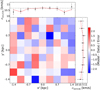 |
Fig. 3. Difference between the best-fit and the observed velocity dispersion in terms of the observed error, for all 9 × 9 kinematic bins. The figure is obtained after fitting the q94v21 library to our mock data consisting of 105 stars with measured line-of-sight velocities in our FOV, assuming an edge-on view. Top and right panels: fit (red full line) obtained along the major and minor axis, respectively. The data points with 68% error bars are shown in black. Black dashed lines indicate the true velocity dispersions from theory (Eq. (4)). |
4.1.2. Downsampling and folding data
We now consider the more realistic case of a sample of 104 stars with measured line-of-sight velocities. We do not change our assumption that the surface brightness profile can be measured without error in our light bins, and therefore here we only investigate the influence of the number of stars with line-of-sight velocities available. To reduce the observed uncertainties on the kinematics we decided to fold the kinematic data (but not the light). Since the system is axisymmetric, we fold our data into the kinematic bins located in the first quadrant. We can simply move each star towards its corresponding kinematic bin without changing its velocity, because our system has an identical Gaussian line-of-sight profile everywhere (see Sect. 2.1). In general, however, one should change the velocities following the assumed symmetry.
Since we fold the kinematic data from 9 × 9 bins of our FOV into the first quadrant, we effectively have 104 stars with measured line-of-sight velocities located in the resulting 5 × 5 kinematic bins. A typical kinematic bin now contains 400 stars with measured line-of-sight velocities on average, and the typical error on the velocity dispersion is ∼0.45 km s−1.
We fit the folded data with the Schwarzschild orbit superposition method and find the MLE for model q90v22 (see Fig. 4). As in the case of 105 stars, and thus as expected, the flattening parameter remains fairly unconstrained. We find a slightly larger mass parameter  km s−1, but v0 = 20 km s−1 is still within the 95% confidence region.
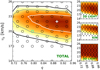 |
Fig. 4. Similar to Fig. 2, but now using 104 stars for the kinematics and using the approach of folding the data from 9 × 9 into 5 × 5 kinematic bins. The parameter inferences are similar, though slightly larger masses are preferred. |
For the best-fit model q90v22 we find  . The contribution of the kinematics (see Eq. (8)) to this value is 13.2. Both values are much lower than in the case of 105 stars, and this can be explained by the decrease in the number of kinematic constraints and the fact that the data have now been folded.
It is encouraging that a more realistic number of stars with measured line-of-sight velocities still gives such tight constraints. Comparing the folded case with 104 stars to the non-folded case with 105 stars, the 2D 68%-probability contours are shifted towards just slightly larger masses. We note that the uncertainty on the mass parameter did not increase.
To further test how the results depend on the number of stars with measured line-of-sight velocities, we even further decreased this number of stars to a sample of 2000 stars. This is the typical size of currently available kinematic datasets used to put constraints on the mass of dSph galaxies (e.g. Walker et al. 2009b; Breddels & Helmi 2013; Hayashi & Chiba 2015). We again fold the data from 9 × 9 into 5 × 5 kinematic bins. The resulting typical error on the velocity dispersion in a kinematic bin is then ∼0.9 km s−1. In this case we find a best-fit model q92v23 ( ,
,  ). The Δχ2 distribution is shown in Fig. 5. The best models are again the most spherical ones, although statistically the flattening parameter remains unconstrained. The region spanned by the contour drawn at Δχ2 = 11.8 is of similar size, but is shifted towards slightly higher masses (Δv0 ∼ 1 km s−1) in comparison to the case of 104 stars. The true q80v20 model is nevertheless still within the inferred 99.7% confidence interval.
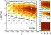 |
Fig. 5. Similar to Fig. 4, now using 2000 stars for the kinematic data. The parameter inferences are similar, though slightly larger masses are inferred (Δv0 ∼ 1 km s−1). |
At first sight it may seem unrealistic that the case of 2000 results in slightly tighter constraints on the parameters of interest. We however note that the differences are minor and that these might be related to the fact that only one data realisation is studied for each case. We also note that not only are the parameters of the potential being fitted in Schwarzschild models but also the orbital weights. This implies that the fitted distribution function can therefore be quite different from one model to the next (especially without the use of regularisation), and the marginalisation over the orbital weights is not being considered when computing the confidence contours on the potential parameters shown in Fig. 5 (also see Magorrian 2006). Nonetheless, when comparing the predicted line-of-sight velocity dispersions for the range of models within these contours (see Fig. 12 in Sect. 4.2.2) weaker constraints are in fact obtained for smaller datasets, as expected.
The weak trend found for smaller samples to result in slightly higher values of v0 may be due to the fact that, for small radii (compared to Rc), the potential (see Eq. (1)) is proportional to ![Mathematical equation: $ v_0^2 [\ln R^2_{\rm c} + (R/R_{\rm c})^2] + (v_0/q)^2 (z/R_{\rm c})^2 $](/articles/aa/full_html/2019/12/aa36196-19/aa36196-19-eq48.gif) . Therefore, there is a weak degeneracy in the term v0/q, that may manifest itself more when the sampling is sparse, and thus lead to a small shift in preferred values of v0 for larger q.
. Therefore, there is a weak degeneracy in the term v0/q, that may manifest itself more when the sampling is sparse, and thus lead to a small shift in preferred values of v0 for larger q.
From the tests performed in this section we conclude that, with a kinematic sampling that follows the light, we cannot aim to constrain the flattening parameter of an isothermal dSph galaxy5, not even if the true functional form of the potential of the system is known. This is likely because the information content in a velocity dispersion regarding the geometric shape of the potential is too small (since σ is constant across the whole system). We can however still reliably constrain the mass parameter of such a system, that is, even though the true flattening parameter remains unknown. This can already be done for a realistic number of stars.
4.2. Axisymmetric NFW models
We have shown that the Schwarzschild method can correctly constrain the mass parameter when the true functional form of the potential of the system is known. Now, we tackle the problem more realistically by allowing a different functional form for the potential of the model. We consider an axisymmetric NFW profile, and follow the parametrisation of Vogelsberger et al. (2008):
![Mathematical equation: $$ \begin{aligned} \Phi _\text{ V}(\tilde{r}) = -4\pi G \rho _0 R^3_{\rm s} \left[ \frac{\ln (1+\tilde{r}/R_{\rm s})}{\tilde{r}} \right], \end{aligned} $$](/articles/aa/full_html/2019/12/aa36196-19/aa36196-19-eq49.gif) (11)
(11)
where Rs is the scale radius and ρ0 a characteristic density parameter. In comparison to the spherical NFW profile, the radius  is replaced by a newly defined radius:
 (12)
(12)
where, for the axisymmetric case,  is the ellipsoidal radius with a and c specifying the relative lengths of the major and minor axes, and where ra is a transition radius. In addition, we require that 2a2 + c2 = 3, such that when a = c = 1, this results in the spherical NFW profile. For r ≫ ra,
  , whereas for r ≪ ra,
  . Therefore, the gravitational potential is axisymmetric in the central regions and becomes spherical in the outer regions. We set the transition radius to ra = 10 kpc. In all our Vogelsberger models we keep the transition radius ra fixed.
To additionally guarantee that the total mass density is positive up to at least the orbits possessing the highest energies in our library (∼50 kpc), the flattening parameter must satisfy c/a ≳ 0.7 for a case with Rs = 1 kpc. For smaller scale radii, increased lower-limit values of c/a are needed to satisfy the positive density criterion.
For convenience, we define a characteristic mass parameter, M1 kpc expressed in units of M⊙, which corresponds to the total enclosed mass within 1 kpc from the centre for a spherical NFW profile with scale radius Rs, that is,
![Mathematical equation: $$ \begin{aligned} M_\text{ NFW}(r = 1 \mathrm{\,kpc} \, \vert \, R_{\rm s}) = 4 \pi \rho _0 {R_{\rm s}}^3 \left[ \ln \left(\frac{R_{\rm s} + r}{R_{\rm s}} \right) - \left( \frac{r}{R_{\rm s} + r} \right) \right]_{1 \mathrm{\,kpc}}. \end{aligned} $$](/articles/aa/full_html/2019/12/aa36196-19/aa36196-19-eq55.gif) (13)
(13)
From this equation we determine the value of ρ0, and it is this value of ρ0 that we use for the axisymmetric Volgelsberger potential in Eq. (11).
4.2.1. The “matched” Vogelsberger model
Before we can test the Schwarzschild orbit superposition method while assuming Vogelsberger mass models, we need to know when a result can be considered satisfactory. Since we could not constrain the flattening parameter for the case when the true functional form of the potential of the system is known, we do not aim to constrain the flattening parameter for the Vogelsberger models. Nevertheless, the corresponding scale radius Rs and mass M1 kpc of our system depend on the c/a-value assumed. In this section we therefore establish what are good parameters for the mass M1 kpc, scale radius Rs, and flattening parameter c/a, such that the properties of the Evans mock galaxy are best reproduced.
Because most stars of our mock galaxy will have projected radii in between 0.5 and 2.0 kpc from the centre, we require that the flattening of the “matched” Vogelsberger model should be comparable to that of the mock galaxy over this region. At a given position we define the Vogelsberger potential flattening qV as the axis ratio of the equipotential contour that goes through that point. For a position (R, z), we therefore define qV(R, z) = zΦ/RΦ, where Φ(R = 0, zΦ) ≡ Φ(RΦ, z = 0) ≡ Φ(R, z). On such an equipotential, it must hold that 
 , and since
  only depends on c/a, then qV(R, z) is independent of our mass parameter and scale radius6. We take values for zΦ from 0.5 to 2.0 kpc in steps of 0.05 kpc along the minor axis and compute the corresponding RΦ values (i.e. the radii where the equipotential contours that belong to zΦ cross the major axis). For a given c/a, we then compute the mean of the absolute differences between the Evans mock galaxy potential flattening (q = 0.8) and the Vogelsberger potential flattening along the defined range for zΦ, that is, we compute: mean(|q − qV(R = 0, zΦ)|). We find that for c/a ≃ 0.776 this average difference is smallest (see left panel of Fig. 6). For our range of zΦ and c/a = 0.776, the Vogelsberger potential flattening increases almost linearly with zΦ, though the gradient is small (0.018 kpc−1).
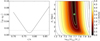 |
Fig. 6. Estimating the “true” parameters of the Vogelsberger system by comparing the differences in potential flattening on the left and the differences in the gradients of the potentials on the right. The comparisons are based on the distance interval from 0.5 up to 2.0 kpc (with steps of 0.05 kpc) from the centre of the galaxy. Left: mean absolute difference of the Vogelsberger potential flattening and the true potential flattening of the mock galaxy as a function of the flattening parameter c/a of the Vogelsberger potential (black line). The grey horizontal line marks the positions where this difference has doubled with respect to the minimum 0.007 at c/a ≃ 0.776. Right: minimisation of the mean of the absolute differences in the gradients of the potential along the major and minor axis (compared to the mock galaxy) by varying the Vogelsberger model parameters M1 kpc and Rs. The figure is obtained after setting the flattening parameter to c/a = 0.776. The colour bar is truncated at 5.0 km s−1. The green circle indicates the location at log10(M1 kpc[M⊙]) ≃ 7.69 and Rs = 4.9 kpc where the differences are minimum (⟨ △ v⟩min = 0.31 km s−1). Grey lines indicate the contours of constant mean absolute differences and are spaced by 1 km s−1. As a proxy for the error on the Vogelsberger parameters, a green contour is drawn where the differences are doubled with respect to the minimum difference. |
Given this value for the flattening parameter c/a, we proceed to obtain the corresponding values for the mass and scale radius of the mock galaxy, now described by the Vogelsberger profile. We do this by comparing  along the major axis and
  along the minor axis with respect to their values for the mock galaxy. We investigate their trends for R- and z-values identical to those used for zΦ previously.
We vary the scale radius and the mass parameter log10(M1 kpc[M⊙]) and compute the mean of the absolute differences with respect to the mock galaxy obtained along the major and minor axis for c/a = 0.776. We denote this by ⟨ △ v⟩≡mean[0.5{abs(Δ|RFR|) + abs(Δ|zFz|)}]. From the right panel of Fig. 6 we infer that ⟨ △ v⟩ is minimum for mass parameter log10(M1 kpc[M⊙]) ≃ 7.69 and scale radius Rs = 4.9 kpc (green circle), although any value with Rs ≥ 2 kpc works well, as ⟨ △ v⟩ does not vary strongly. To be able to compare these findings to the results from our Schwarzschild models (see Sect. 4.2.2), we estimate the error on these “true” parameters by considering those locations where ⟨ △ v⟩ changes by a factor of two with respect to its minimum value (green contour). The mass parameter is then within the range [7.63, 7.73], the scale radius larger than 2.4 kpc. For the smaller scale radii (Rs < 2 kpc) slightly higher values for the characteristic mass parameter would be preferred, but ⟨ △ v⟩ is also larger in such cases. We note that the NFW mass value that we estimated immediately above corresponds well with the mass enclosed within 1 kpc of a spherical Evans model with Rc = 1 kpc and v0 = 20 km s−1 (as assumed in Sect. 2), since then log10(M1 kpc,Evans[M⊙]) ≃ 7.67.
Although we do not constrain the flattening parameter, we can investigate how the parameters of our matched Vogelsberger model would change if different values for c/a were taken. Setting c/a = 0.70 results in ⟨ △ v⟩ = 0.32 km s−1 for its minimum at log10(M1 kpc[M⊙]) ≃ 7.69 and Rs = 4.4 kpc, and setting c/a = 0.85 results in ⟨ △ v⟩ = 0.37 km s−1 for log10(M1 kpc[M⊙]) ≃ 7.69 and Rs = 5.1 kpc. Even for a spherical potential, i.e. c/a = 1.0, we find the minimum ⟨ △ v⟩ = 0.62 km s−1 to be located at log10(M1 kpc[M⊙]) ≃ 7.68 and Rs = 6.1 kpc. The corresponding Vogelsberger mass parameter is thus not affected by the choice of c/a. The corresponding scale radius only increases slightly for larger values for the flattening parameter (i.e. rounder shapes), though the effect is rather small. In addition, the grey contours, which are drawn at fixed ⟨ △ v⟩, span very similar regions for different values of c/a.
In Fig. 7 we compare the potential of the matched Vogelsberger model to the true Evans potential of our mock galaxy. In the left panel we show the gradients of the potentials along the major and minor axis. We note that the Evans model seems to have lower |RFR| and |zFz| for R ≲ 1 kpc and z ≲ 0.75 kpc, respectively, than the matched NFW model. In the panel on the right we confirm that the potential flattening parameter is matched quite well by showing isopotential contours. Both panels reveal that only in the centre (< 0.7 kpc) and at distances larger than 3 kpc do the gradients of both potentials start to deviate from each other.
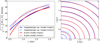 |
Fig. 7. Left: major (full lines) and minor (dashed lines) axis gradients of the potential as functions of R and z, respectively, for the true Evans model (red) and for the matched Vogelsberger model with c/a ≃ 0.776, Rs ≃ 4.9 kpc and log10(M1 kpc[M⊙]) ≃ 7.69 (blue). Right: comparison of the isopotential contours for the true Evans model (red) and the matched Vogelsberger model (blue). For the purpose of this figure the zero-point of the potential is chosen here such that ΦE = ΦV at (R, z) = (1, 0) kpc. For each potential, contours are drawn at the positions where Φ has changed in steps of 50 km2 s−2. In the region from 0.7 up to 2 kpc the matched Vogelsberger model follows well the true Evans potential. For more inner radii the (cusped) Vogelsberger models cannot reproduce the (less steep) cored behaviour of the Evans potential. |
In summary, the matched Vogelsberger system can be described by ![Mathematical equation: $ {\log _{10}}({M_{1 {\rm{kpc}}}}[{M_ \odot }]) \simeq 7.69_{ - 0.06}^{ + 0.04} $](/articles/aa/full_html/2019/12/aa36196-19/aa36196-19-eq61.gif) and by Rs ≳ 2.4 kpc (with its most likely value at Rs = 4.9 kpc) for c/a = 0.776.
and by Rs ≳ 2.4 kpc (with its most likely value at Rs = 4.9 kpc) for c/a = 0.776.
4.2.2. Fitting Vogelsberger models with the Schwarzschild method: exploring different sample sizes
Since we were not able to constrain the flattening parameter when the functional form of the potential of the system was known (see Sect. 4.1), we cannot expect to constrain the flattening parameter if we examine a different functional form for the model. We set c/a = 0.80, which is equal to the observed axial ratio in the light, and subsequently find the inferences on the mass log10(M1 kpc[M⊙]) and scale radius Rs. We initially make a grid in (log10(M1 kpc, Rs)-space, where Rs ranges from 1 to 8 kpc with steps of ΔRs = 1 kpc, while for the characteristic mass we take steps of 0.05 for values from log10(M1 kpc[M⊙]) = 7.55 to log10(M1 kpc[M⊙]) = 7.85, that is, spanning a factor of only two in mass. Later, we also decided to sample log10(M1 kpc[M⊙]) = [7.68,7.72] for Rs ∈ [1.5, 7.5] kpc with a similar ΔRs step.
To be more efficient we decrease the number of orbits compared to Sect. 4.1 and set Nener = 24, NI2 = 24, and NI3 = 8, such that a total of 24 × 24 × 8 × 53 = 576 000 suborbits are integrated and 2 × 24 × 24 × 8 = 9216 orbital weights are determined. We find this gives good results in terms of recovery of the light profile and kinematics. In addition we also add regularisation terms to the fit in this more realistic experiment: by applying regularisation we set additional constraints such that the orbital weights are more smoothly distributed, that is, in a more physical way (as the weights relate to the distribution function, which itself is expected to be smooth). More details on the concept of regularisation and its effects can be found in Appendix C.
We present the results following the same structure of Sect. 4.1 and name the Vogelsberger models by MxxxRsyyy, where xxx = 100 log10(M1 kpc[M⊙]) and yyy = 100 Rs (in kpc). We discuss how well we can recover the characteristic parameters of the Vogelsberger potential for mock datasets containing 105, 104, and 2000 stars.
We start with the case of a kinematic dataset containing 105 stars. We use 9 × 9 kinematic bins, but no folding. For this case, we find that model M772Rs250 provides the best fit ( ). Figure 8 shows that this model accurately reproduces the mock velocity dispersions in all kinematic bins (since
  , which results in 0.68 per kinematic constraint). The fit is of comparable quality to the best-fit Evans model (for the same case) although the light is recovered slightly less well, which may be driven by the smaller number of orbits being used now, the choice of a different (and incorrect) potential form, or by adding regularisation in the fit.
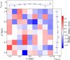 |
Fig. 8. Difference between the best-fit Vogelsberger model (M772Rs250, blue line in the subpanels) and the observed velocity dispersion when applying the Schwarzschild method in 9 × 9 kinematic bins to our mock dataset consisting of 105 stars in the FOV (see Fig. 3 for a comparison). |
Figure 9 shows the resulting Δχ2 distribution in (log10(M1 kpc), Rs)-parameter space. The scale radius of the Vogelsberger potential is constrained to  kpc and the mass parameter to
 ![Mathematical equation: $ {\log _{10}}({M_{1 {\rm{kpc}}}}[{M_ \odot }]) = 7.72_{ - 0.01}^{ + 0.01} $](/articles/aa/full_html/2019/12/aa36196-19/aa36196-19-eq65.gif) . The Schwarzschild model thus prefers values towards the lower end for the scale radius and a mass parameter that agrees well with of our expectations. The panels on the right show the Δχ2-landscapes when only considering
. The Schwarzschild model thus prefers values towards the lower end for the scale radius and a mass parameter that agrees well with of our expectations. The panels on the right show the Δχ2-landscapes when only considering  (top),
  (top-middle),
  (bottom-middle), or
  (bottom). The total Δχ2-landscape is dominated by the kinematics and 2D light.
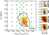 |
Fig. 9. Confidence intervals for the axisymmetric Vogelsberger model in (log10(M1 kpc, Rs) (after fixing c/a = 0.8) for a kinematic dataset with 105 stars and 9 × 9 kinematic bins. The Δχ2 = [2.3, 6.18, 11.8]-contours are in white, grey, and black, respectively. The best-fit model is indicated by the white cross, while the expectations are given by the green contour (identical to that shown in Fig. 6). The mass parameter is well constrained and models with Rs ≤ 2.0 kpc are strongly disfavoured, consistent with our expectations. The small panels on the right show the Δχ2 landscapes when only considering |


As shown in Fig. 10, similar best-fit parameters are obtained for a smaller mock kinematic dataset containing 104 stars and folding the data into 5 × 5 kinematic bins. The mass and scale parameters are constrained to  kpc and
 ![Mathematical equation: $ {\log _{10}}({M_{1 {\rm{kpc}}}}[{M_ \odot }]) = 7.75_{ - 0.03}^{ + 0.05} $](/articles/aa/full_html/2019/12/aa36196-19/aa36196-19-eq75.gif) . For the best-fit model M775Rs300,
. For the best-fit model M775Rs300,  and
and  , or 0.339 per kinematic constraint on average. This
  is lower than for the case of 105 stars, likely because we folded the data. In comparison to the best-fit Evans model, the quality of the fit of the kinematics is slightly worse but is still very good.
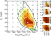 |
Fig. 10. Similar to Fig. 9, but now after fitting mock kinematic data consisting of 104 stars and folding into 5 × 5 kinematic bins. The decrease in sample size (by a factor of ten) has led to a slight increase by the area spanned by the probability contours, although the inference on the mass parameter is still very good and only changed to slightly higher masses. |
When decreasing the sample size of the kinematics even further to 2000 stars, we find that models with low values for Rs and larger log10(M1 kpc[M⊙]) are now preferred, as shown in Fig. 11, although the 95%-confidence region still overlaps with the values for the parameters of the matched Vogelsberger model. For the best-fit model M780Rs100, we find  and
and  , or 0.672 per kinematic constraint on average. We infer
  kpc and
 ![Mathematical equation: $ {\log _{10}}({M_{{\rm{1}} {\rm{kpc}}}}[{M_ \odot }]) = 7.80_{ - 0.01}^{ + 0.02} $](/articles/aa/full_html/2019/12/aa36196-19/aa36196-19-eq82.gif) for the Vogelsberger parameters.
for the Vogelsberger parameters.
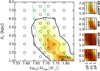 |
Fig. 11. As in Fig. 10, but now for a kinematic dataset with 2000 stars. We note how the confidence contours follow the shape of the green contour (derived in Fig. 6). |
It is interesting to note that the shape of the confidence contours obtained from the Schwarzschild method for all sample sizes follows very closely the shape of the contours of ⟨Δv⟩ depicted in Fig. 6. We reiterate that the quantity ⟨Δv⟩ is a proxy for the difference in enclosed mass between the Evans and Vogelsberger models. This implies that the Schwarzschild method is actually very sensitive to enclosed mass, and is identifying the set of Vogelsberger models that best follow the true underlying mass distribution. Also interesting is that the trend favouring larger values of the mass parameter when decreasing sample size is present both for the Evans and the Vogelsberger models.
We compare the Evans and Vogelsberger best-fit models to the observed velocity dispersions in Fig. 12. The left and right panels compare the behaviour on the major and minor axes, respectively, for different sample sizes for the kinematics: 105, 104, and 2000 stars (in the top, middle, and bottom rows, respectively). The shaded areas enclose the minimum and maximum velocity dispersions for the evaluated models within the Δχ2 = [2.3, 6.18, 11.8]-contours. These comparisons show that the Evans models fit the kinematics slightly better but that nearly equally good fits are provided by the Vogelsberger models (except in along the minor axis for the smallest dataset, bottom right panel).
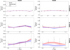 |
Fig. 12. Comparison of the results from the Schwarzschild modelling fits to the observed velocity dispersion along the major (left column) and minor (right column) axis. From top to bottom: best-fit Evans (red line) and Vogelsberger (blue line) models for kinematic datasets containing N = 105, N = 104, and 2000 stars, respectively. The shaded regions denote the error bands computed as described in the text. Black dotted lines indicate the input (theoretical, Eq. (4)) velocity dispersions. |
From the analyses presented in this section we may thus conclude that the Schwarzschild modelling technique is sensitive to the mass enclosed and that it is successful in well constraining the mass parameter of the models, even if the functional form of the potential of the system is not known.
5. Discussion and conclusions
We explored the ability of Schwarzschild’s orbit superposition method to characterise the intrinsic properties of an axisymmetric dSph galaxy, such as its mass, scale radius, and flattening. We did this by setting up an isothermal Sculptor-like mock galaxy that is flattened in both the luminous and dark components. We showed that Schwarzschild’s method, applied to mock datasets with a realistic number of stars with measured radial velocities distributed following the luminosity profile of the system, is successful in recovering the characteristic mass parameter of the underlying (true) logarithmic potential, even if the potential flattening is not known. On the other hand, we find that we cannot put constraints on the flattening parameter.
Most likely, our inability to constrain the flattening is the consequence of our choice of the specific Evans model for our mock galaxy. In this model with a distribution function that is ergodic, the line-of-sight velocity profile is exactly the same everywhere and depends on the mass parameter only. This means that the kinematics are independent of the inclination and flattening, and the light alone does not contain enough information to constrain the flattening parameter.
One might also argue that it might not be optimal for a spectroscopic survey to sample stars according to the light profile of the system. In fact, slightly better results were obtained when the dataset with radial velocities provided an equal number of stars to each kinematic bin. In addition, just ∼30% of the light of the system is within our FOV for the specific Evans model used in this work. It might be possible that better results could be obtained with a more realistic and general distribution function (i.e. non-ergodic) applied to a galaxy for which the kinematic tracers cover the full system well and better sample the outskirts.
Since in reality the functional form of the potential of the system is not known, we also explored the case in which we assume an axisymmetric NFW model. We first determined the values of the parameters of the matched NFW model that mimics the mock galaxy best by comparing some basic properties (potential flattening and gradients in the potential). We found that even in this case, in which the orbits that form the building blocks of Schwarzschild’s method are integrated in the incorrect potential, we can retrieve the correct characteristic mass and scale parameters.
We explored the dependencies of our results on the sizes of the data samples used, and find that a decrease in the number of stars with line-of-sight velocities only slightly affects the determination of the characteristic parameters of the model. For the smallest kinematic sample considered, with 2000 stars, the inference on the mass of the matched NFW model is somewhat poorer, but the true value differs by only 20% from the best-fit and also lies within the 95% confidence interval.
We checked that our results are not strongly dependent on the choices of the number of orbits in the orbit libraries, the number of kinematic or light bins, or the number of velocity bins, for example. Furthermore, we also briefly investigated the distribution functions for the the best-fit models, and found that, particularly when regularisation is included, they are quite similar to the distribution function of the mock dSph galaxy.
In conclusion, it is promising that the mass of our flattened system can be recovered to such a degree even if the flattening parameter is unknown. This is also aligned with the results of Kowalczyk et al. (2018), who applied their spherical Schwarzschild models on non-spherical objects. To some extent, this provides us with more confidence regarding previously reported estimates of the mass of dSph galaxies obtained assuming spherical symmetry.
Nor is this distribution function ideal as we see below, because it provides very little information on the symmetries of the system.
For an extended system like the one studied here, it would be better to use a larger FOV, or to have multiple pointings. The size of the FOV used here is however reasonable for dSph galaxies like Sculptor.
We note that the Schwarzschild code by van den Bosch et al. (2008) was developed to model triaxial systems, and therefore also generates initial conditions for box orbits, which have zero time-averaged angular momentum and which can cross the centre (Schwarzschild 1979, 1993). In an axisymmetric potential Lz is conserved and such box orbits will therefore never attain velocities in the azimuthal direction. As this could cause non-axisymmetries in our model we do not specifically generate box orbits.
We used the scipy.interpolate.LinearNDInterpolator to interpolate the Δχ2. Although using linear interpolation might not be optimal, it does not strongly affect the quantitative results of the paper.
Slightly better results can be obtained by sampling uniformly with distance, see Appendix B.
More precisely,  depends on ra and rE(c/a), but we have chosen to fix the value of ra (and make it independent of Rs).
With respect to Breddels et al. (2013), small corrections to the equations are made. The updates concern Eqs. (A.4), (A.8), and (A.10).
Acknowledgments
We thank the anonymous referee whose comments helped to improve the manuscript. We also thank R. van den Bosch for supplying us the Schwarzschild code and L. Posti and P.T. de Zeeuw for many useful discussions regarding the project. A.H. acknowledges financial support from a VICI grant from the Netherlands Organisation for Scientific Research, NWO. For the analysis, the following software packages have been used: NumPy (Oliphant 2015), matplotlib (Hunter 2007), Jupyter Notebook (Kluyver et al. 2016).
References
- Battaglia, G., Tolstoy, E., Helmi, A., et al. 2006, A&A, 459, 423 [NASA ADS] [CrossRef] [EDP Sciences] [Google Scholar]
- Battaglia, G., Helmi, A., Tolstoy, E., et al. 2008a, ApJ, 681, L13 [NASA ADS] [CrossRef] [Google Scholar]
- Battaglia, G., Irwin, M., Tolstoy, E., et al. 2008b, MNRAS, 383, 183 [NASA ADS] [CrossRef] [MathSciNet] [Google Scholar]
- Battaglia, G., Tolstoy, E., Helmi, A., et al. 2011, MNRAS, 411, 1013 [NASA ADS] [CrossRef] [MathSciNet] [Google Scholar]
- Battaglia, G., Helmi, A., & Breddels, M. 2013, New A Rev., 57, 52 [Google Scholar]
- Binney, J., & Tremaine, S. 2008, Galactic Dynamics, 2nd edn. (Princeton: Princeton University Press) [Google Scholar]
- Boylan-Kolchin, M., Bullock, J. S., & Kaplinghat, M. 2011, MNRAS, 415, L40 [CrossRef] [Google Scholar]
- Breddels, M. A., & Helmi, A. 2013, A&A, 558, A35 [NASA ADS] [CrossRef] [EDP Sciences] [Google Scholar]
- Breddels, M. A., Helmi, A., van den Bosch, R. C. E., van de Ven, G., & Battaglia, G. 2013, MNRAS, 433, 3173 [NASA ADS] [CrossRef] [Google Scholar]
- Brooks, A. M., Kuhlen, M., Zolotov, A., & Hooper, D. 2013, ApJ, 765, 22 [Google Scholar]
- Evans, N. W. 1993, MNRAS, 260, 191 [NASA ADS] [Google Scholar]
- Evans, N. W., An, J., & Walker, M. G. 2009, MNRAS, 393, L50 [NASA ADS] [Google Scholar]
- Hayashi, K., & Chiba, M. 2012, ApJ, 755, 145 [NASA ADS] [CrossRef] [Google Scholar]
- Hayashi, K., & Chiba, M. 2015, ApJ, 810, 22 [NASA ADS] [CrossRef] [Google Scholar]
- Hayashi, K., & Obata, I. 2019, MNRAS, in press, [arXiv:1902.03054] [Google Scholar]
- Hayashi, K., Ichikawa, K., Matsumoto, S., et al. 2016, MNRAS, 461, 2914 [NASA ADS] [CrossRef] [Google Scholar]
- Hui, L. 2001, Phys. Rev. Lett., 86, 3467 [NASA ADS] [CrossRef] [Google Scholar]
- Hunter, J. D. 2007, Comput. Sci. Eng., 9, 90 [NASA ADS] [CrossRef] [Google Scholar]
- Irwin, M., & Hatzidimitriou, D. 1995, MNRAS, 277, 1354 [NASA ADS] [CrossRef] [Google Scholar]
- Jing, Y. P., & Suto, Y. 2002, ApJ, 574, 538 [NASA ADS] [CrossRef] [Google Scholar]
- Kim, S. Y., Peter, A. H. G., & Hargis, J. R. 2018, Phys. Rev. Lett., 121, 211302 [NASA ADS] [CrossRef] [Google Scholar]
- Kluyver, T., Ragan-Kelley, B., Pérez, F., et al. 2016, in Positioning and Power in Academic Publishing: Players, Agents and Agendas, eds. F. Loizides, & B. Scmidt (IOS Press), 87 [Google Scholar]
- Klypin, A., Kravtsov, A. V., Valenzuela, O., & Prada, F. 1999, ApJ, 522, 82 [Google Scholar]
- Kowalczyk, K., Łokas, E. L., & Valluri, M. 2017, MNRAS, 470, 3959 [NASA ADS] [CrossRef] [Google Scholar]
- Kowalczyk, K., Łokas, E. L., & Valluri, M. 2018, MNRAS, 476, 2918 [NASA ADS] [CrossRef] [Google Scholar]
- Magorrian, J. 2006, MNRAS, 373, 425 [NASA ADS] [CrossRef] [Google Scholar]
- Massari, D., Breddels, M. A., Helmi, A., et al. 2018, Nat. Astron., 2, 156 [NASA ADS] [CrossRef] [Google Scholar]
- Massari, D., Helmi, A., Mucciarelli, A., et al. 2019, A&A, in press, https://doi.org/10.1051/0004-6361/201935613 [Google Scholar]
- Mateo, M. L. 1998, ARA&A, 36, 435 [NASA ADS] [CrossRef] [Google Scholar]
- McConnachie, A. W. 2012, AJ, 144, 4 [NASA ADS] [CrossRef] [Google Scholar]
- Merrifield, M. R., & Kent, S. M. 1990, AJ, 99, 1548 [NASA ADS] [CrossRef] [Google Scholar]
- Moore, B., Ghigna, S., Governato, F., et al. 1999, ApJ, 524, L19 [Google Scholar]
- Navarro, J. F., Frenk, C. S., & White, S. D. M. 1996, ApJ, 462, 563 [NASA ADS] [CrossRef] [Google Scholar]
- Oliphant, T. E. 2015, Guide to NumPy, 2nd edn. (USA: CreateSpace Independent Publishing Platform) [Google Scholar]
- Press, W. H., Teukolsky, S. A., Vetterling, W. T., & Flannery, B. P. 1992, Numerical Recipes: The Art of Scientific Computing, 2nd edn. (New York, NY, USA: Cambridge University Press) [Google Scholar]
- Richardson, T., & Fairbairn, M. 2013, MNRAS, 432, 3361 [NASA ADS] [CrossRef] [Google Scholar]
- Schwarzschild, M. 1979, ApJ, 232, 236 [NASA ADS] [CrossRef] [Google Scholar]
- Schwarzschild, M. 1993, ApJ, 409, 563 [NASA ADS] [CrossRef] [Google Scholar]
- Strigari, L. E., Koushiappas, S. M., Bullock, J. S., et al. 2008, ApJ, 678, 614 [NASA ADS] [CrossRef] [Google Scholar]
- Strigari, L. E., Frenk, C. S., & White, S. D. M. 2017, ApJ, 838, 123 [NASA ADS] [CrossRef] [Google Scholar]
- van den Bosch, R. C. E., van de Ven, G., Verolme, E. K., Cappellari, M., & de Zeeuw, P. T. 2008, MNRAS, 385, 647 [NASA ADS] [CrossRef] [Google Scholar]
- Vera-Ciro, C. A., Sales, L. V., Helmi, A., & Navarro, J. F. 2014, MNRAS, 439, 2863 [NASA ADS] [CrossRef] [Google Scholar]
- Vogelsberger, M., White, S. D. M., Helmi, A., & Springel, V. 2008, MNRAS, 385, 236 [NASA ADS] [CrossRef] [Google Scholar]
- Walker, M. G., Mateo, M., Olszewski, E. W., et al. 2007, ApJ, 667, L53 [NASA ADS] [CrossRef] [Google Scholar]
- Walker, M. G., Mateo, M., & Olszewski, E. W. 2009a, AJ, 137, 3100 [NASA ADS] [CrossRef] [Google Scholar]
- Walker, M. G., Mateo, M., Olszewski, E. W., et al. 2009b, ApJ, 704, 1274 [NASA ADS] [CrossRef] [Google Scholar]
- Walker, M. G., Olszewski, E. W., & Mateo, M. 2015, MNRAS, 448, 2717 [NASA ADS] [CrossRef] [Google Scholar]
- Wetzel, A. R., Hopkins, P. F., Kim, J.-H., et al. 2016, ApJ, 827, L23 [NASA ADS] [CrossRef] [Google Scholar]
- Wolf, J., Martinez, G. D., Bullock, J. S., et al. 2010, MNRAS, 406, 1220 [NASA ADS] [Google Scholar]
- Zolotov, A., Brooks, A. M., Willman, B., et al. 2012, ApJ, 761, 71 [Google Scholar]
Appendix A: Generating a mock kinematic dataset with realistic errors
Like in Breddels et al. (2013)7, we define vi as the true line-of-sight velocity of star i and ϵi as the (true and unknown) measurement error on that star. Therefore, vi + ϵi is the observed velocity of star i. We note that the expectation values for the moments of the measurement errors, which are drawn from a Gaussian distribution with σ = 2 km s−1, are given by: ![Mathematical equation: $ E\left[ \langle \epsilon^{n}_{i} \rangle \right]= E \left[ \epsilon^{n}_{i} \right] = 0 $](/articles/aa/full_html/2019/12/aa36196-19/aa36196-19-eq84.gif) for odd n and
for odd n and ![Mathematical equation: $ s_n \equiv E \left[ \langle \epsilon^{n}_{i} \rangle \right] = E \left[\epsilon^{n}_{i} \right] = (n-1)!!\sigma^n $](/articles/aa/full_html/2019/12/aa36196-19/aa36196-19-eq85.gif) for even n. In our terminology,
for even n. In our terminology, ![Mathematical equation: $ \hat{\mu_n} = E[\langle v^{n}_{i} \rangle] = E[v^{n}_{i}] $](/articles/aa/full_html/2019/12/aa36196-19/aa36196-19-eq86.gif) denotes the true nth moment, μn is its estimator, and the observed nth moment is
denotes the true nth moment, μn is its estimator, and the observed nth moment is  for a sample of N stars in a given positional bin on the sky (i.e. kinematic bin).
Since we want to know the true value of the moments, that is, without measurement errors, we compute the estimators of the true moments. We also use raw moments (i.e. not taken about the mean velocities), and in what follows, we use the term “moments” to refer to “raw moments”. Since we can only in practise compute the estimators of the true moments, we replaced  with μn in the right-hand side of the following equations. The first four moment estimators are then given by:
 (A.1)
(A.1)
 (A.2)
(A.2)
 (A.3)
(A.3)
and
 (A.4)
(A.4)
To compute the error on these moments, we compute the square root of the variance of the moments; ![Mathematical equation: $ \mathrm{Var}(\hat{\mu_n}) \approx \mathrm{Var}(\mu_n) \approx \mathrm{Var}(m_n) = E[{m_n}^2] - (E[m_n])^2 $](/articles/aa/full_html/2019/12/aa36196-19/aa36196-19-eq93.gif) :
:
![Mathematical equation: $$ \begin{aligned} \mathrm{Var}(\mu _1)&= \frac{\mu _2 + s_2 - \mu _1^2}{N} \nonumber \\&= \frac{1}{N} \left\{ \frac{1}{N} \sum \limits ^N_{i=1} (v_i + \epsilon _i)^2 - \left[ \frac{1}{N} \sum \limits ^N_{i=1} (v_i + \epsilon _i) \right]^2 \right\} , \end{aligned} $$](/articles/aa/full_html/2019/12/aa36196-19/aa36196-19-eq94.gif) (A.5)
(A.5)
![Mathematical equation: $$ \begin{aligned} \mathrm{Var}(\mu _2)&= \frac{1}{N} \left[ \mu _4 - \mu _2^2 + 4 \mu _2 s_2 + 2s^2_2\right] \nonumber \\&= \frac{1}{N} \left\{ \frac{1}{N} \sum \limits ^N_{i=1} (v_i + \epsilon _i)^4 - \left[ \frac{1}{N} \sum \limits ^N_{i=1} (v_i + \epsilon _i)^2 \right]^2 \right\} , \end{aligned} $$](/articles/aa/full_html/2019/12/aa36196-19/aa36196-19-eq95.gif) (A.6)
(A.6)
![Mathematical equation: $$ \begin{aligned} \mathrm{Var}(\mu _3)&= \frac{1}{N} \left[ \mu _6 +15\mu _4 s_2 + 45\mu _2 s^2_2 + 15s^3_2 - \mu ^2_3 \right.\nonumber \\&\quad -\left.6 \mu _3 \mu _1 s_2 - 9\mu ^2_1 s^2_2 \right] \nonumber \\&= \frac{1}{N} \left\{ \frac{1}{N} \sum \limits ^N_{i=1} (v_i + \epsilon _i)^6 - \left[ \frac{1}{N} \sum \limits ^N_{i=1} (v_i + \epsilon _i)^3 \right]^2 \right\} , \end{aligned} $$](/articles/aa/full_html/2019/12/aa36196-19/aa36196-19-eq96.gif) (A.7)
(A.7)
and
![Mathematical equation: $$ \begin{aligned} \begin{split} \mathrm{Var}(\mu _4)&= \frac{1}{N} \left[ \mu _8 + 28\mu _6 s_2 -\mu ^2_4 - 12 \mu _4 \mu _2 s_2 + 204\mu _4 s^2_2 \right. \\&\quad - \left. 36\mu ^2_2 s^2_2 + 384\mu _2 s^3_2 + 96s^4_2\right] \\&= \frac{1}{N} \left\{ \frac{1}{N} \sum \limits ^N_{i=1} (v_i + \epsilon _i)^8 - \left[ \frac{1}{N} \sum \limits ^N_{i=1} (v_i + \epsilon _i)^4 \right]^2 \right\} , \end{split} \end{aligned} $$](/articles/aa/full_html/2019/12/aa36196-19/aa36196-19-eq97.gif) (A.8)
(A.8)
where the errors on the third and fourth moment estimators also depend on:
 (A.9)
(A.9)
and
 (A.10)
Clearly, the errors on the moments decrease when the number of stars in a kinematic bin increases.
Appendix B: The effect of the sampling of line-of-sight velocities
In the main text we drew samples of line-of-sight velocities that follow the light distribution of the mock galaxy. Here we show the results of applying the Schwarzschild modelling technique to a kinematic dataset consisting of 105 stars, but this time distributed such that each kinematic bin has an equal number of stars, therefore effectively increasing the relative importance of the kinematic bins near the edges of our FOV with respect to the most central kinematic bins. This is because the errors on the moments decrease with increasing numbers of stars in a kinematic bin. In reality one might also consider probing larger radii.
Figure B.1 presents the inference on the mass and flattening parameter and should be compared to Figs. 2 and 3. As can be observed, we have very similar inferences with the best-fit flattening parameter slightly moved into the direction of its input/true value. Nonetheless, this remains fairly unconstrained.
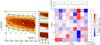 |
Fig. B.1. Left: confidence intervals after fitting the Evans models to a new realization of the dataset containing 105 stars. This time we ensure an equal number of stars per kinematic bin. The inference on the mass parameter remains the same. The flattening parameter remains unconstrained but has slightly shifted into the direction of the correct flattening parameter. Right: velocity dispersion profile for the best-fit model q86v21. |
Appendix C: Regularisation
The solution of our minimisation problem may result in a distribution of orbital weights that is rapidly varying or shows sharp discontinuities. Such a distribution would not be physical. Therefore we make the distribution of the orbital weights smoother by adding extra terms to the χ2-fitting algorithm such that a new quantity  is minimised:
 (C.1)
(C.1)
This procedure is called regularisation. The regularisation strength is chosen such that the orbital weights are forced to change smoothly from one neighbouring orbit to the next, while finding similar values for the best-fit characteristic parameters. In addition, the confidence contours should not be significantly shaped by the  -term. We refer the reader to van den Bosch et al. (2008) for more information about the exact implementation, in particular to Eqs. (28) and (29) of that paper. These equations require the 3D stellar density profile. For this work we assumed to know ρlum (see Eq. (2)). In reality one needs the inclination angle to transform the observed surface brightness profile into the stellar density profile.
In the bottom panels of Fig. C.1, we show the effect of adding regularisation for the Evans q80v20 model (i.e. this is the true model) on the distribution of angular momentum around the symmetry axis (Lz). The distributions can be compared to those of the q80v20 model without regularisation (top rows). Here we show the example with 105 stars with line-of-sight velocities. The modelled distribution functions (blue) are generally smoother when regularisation is used. As a reference we also include the distributions for a realization of the mock galaxy (red). The model reproduces the mock distribution reasonably well, though some differences exist. The fact that only ∼30% of the total number of stars of the mock galaxy end up in our FOV might play a role here, in addition to the fact that we have discretized the data (by using kinematic bins, and by modelling only the first four velocity moments).
 |
Fig. C.1. Orbital distributions of angular momentum around the symmetry axis, i.e. Lz, for fixed energy slices corresponding to circular orbits at x = 0.4 (left), x = 1.0 (middle), and x = 1.8 kpc (right). We note the different axes ranges for the panels of each column. In the top row we show the distributions for the true Evans model q80v20 (blue) obtained after fitting a kinematic dataset of 105 stars (see Sect. 4.1) and for a realization of the mock galaxy (red, here containing 4 × 10⁵ stars in total). The effect of adding regularisation to the fit is shown in the bottom panels. Adding regularisation makes the recovered distribution smoother and more similar to the true distribution. |
All Figures
|
Fig. 1. Surface brightness profile of our mock galaxy in an edge-on view. The black horizontal and vertical lines show the boundaries of the kinematic bins. We only show the positive quadrant of our FOV (x′> 0 kpc, y′> 0 kpc). The yellow contours correspond to the isophotes of the system (q* = q = 0.8). In the top panel we have plotted the surface brightness normalised to its central value as function of x′, i.e. along the (projected) major axis of the galaxy. |
| In the text | |
|
Fig. 2. Δχ2-distribution of the characteristic parameters q and v0 of the Evans models obtained after applying the Schwarzschild method. In this case our mock kinematic data consist of 105 stars inside the FOV (3 × 3 kpc). We use 9 × 9 kinematic bins and assume the functional form of the potential of the system and inclination are known. The black circles show the locations where the Schwarzschild models were evaluated. The green circle indicates the input parameters of the mock system. The best-fit model is indicated by the white cross and recovers the mock galaxy mass parameter. In white, grey, and black we show the Δχ2 = [2.3, 6.18, 11.8]-contours, respectively. The coloured landscape on the left shows interpolated Δχ2-values, and goes up to a maximum of Δχ2 = 10. On the right we show the Δχ2-landscapes when decomposing the landscape into |
| In the text | |
|
Fig. 3. Difference between the best-fit and the observed velocity dispersion in terms of the observed error, for all 9 × 9 kinematic bins. The figure is obtained after fitting the q94v21 library to our mock data consisting of 105 stars with measured line-of-sight velocities in our FOV, assuming an edge-on view. Top and right panels: fit (red full line) obtained along the major and minor axis, respectively. The data points with 68% error bars are shown in black. Black dashed lines indicate the true velocity dispersions from theory (Eq. (4)). |
| In the text | |
|
Fig. 4. Similar to Fig. 2, but now using 104 stars for the kinematics and using the approach of folding the data from 9 × 9 into 5 × 5 kinematic bins. The parameter inferences are similar, though slightly larger masses are preferred. |
| In the text | |
|
Fig. 5. Similar to Fig. 4, now using 2000 stars for the kinematic data. The parameter inferences are similar, though slightly larger masses are inferred (Δv0 ∼ 1 km s−1). |
| In the text | |
|
Fig. 6. Estimating the “true” parameters of the Vogelsberger system by comparing the differences in potential flattening on the left and the differences in the gradients of the potentials on the right. The comparisons are based on the distance interval from 0.5 up to 2.0 kpc (with steps of 0.05 kpc) from the centre of the galaxy. Left: mean absolute difference of the Vogelsberger potential flattening and the true potential flattening of the mock galaxy as a function of the flattening parameter c/a of the Vogelsberger potential (black line). The grey horizontal line marks the positions where this difference has doubled with respect to the minimum 0.007 at c/a ≃ 0.776. Right: minimisation of the mean of the absolute differences in the gradients of the potential along the major and minor axis (compared to the mock galaxy) by varying the Vogelsberger model parameters M1 kpc and Rs. The figure is obtained after setting the flattening parameter to c/a = 0.776. The colour bar is truncated at 5.0 km s−1. The green circle indicates the location at log10(M1 kpc[M⊙]) ≃ 7.69 and Rs = 4.9 kpc where the differences are minimum (⟨ △ v⟩min = 0.31 km s−1). Grey lines indicate the contours of constant mean absolute differences and are spaced by 1 km s−1. As a proxy for the error on the Vogelsberger parameters, a green contour is drawn where the differences are doubled with respect to the minimum difference. |
| In the text | |
|
Fig. 7. Left: major (full lines) and minor (dashed lines) axis gradients of the potential as functions of R and z, respectively, for the true Evans model (red) and for the matched Vogelsberger model with c/a ≃ 0.776, Rs ≃ 4.9 kpc and log10(M1 kpc[M⊙]) ≃ 7.69 (blue). Right: comparison of the isopotential contours for the true Evans model (red) and the matched Vogelsberger model (blue). For the purpose of this figure the zero-point of the potential is chosen here such that ΦE = ΦV at (R, z) = (1, 0) kpc. For each potential, contours are drawn at the positions where Φ has changed in steps of 50 km2 s−2. In the region from 0.7 up to 2 kpc the matched Vogelsberger model follows well the true Evans potential. For more inner radii the (cusped) Vogelsberger models cannot reproduce the (less steep) cored behaviour of the Evans potential. |
| In the text | |
|
Fig. 8. Difference between the best-fit Vogelsberger model (M772Rs250, blue line in the subpanels) and the observed velocity dispersion when applying the Schwarzschild method in 9 × 9 kinematic bins to our mock dataset consisting of 105 stars in the FOV (see Fig. 3 for a comparison). |
| In the text | |
|
Fig. 9. Confidence intervals for the axisymmetric Vogelsberger model in (log10(M1 kpc, Rs) (after fixing c/a = 0.8) for a kinematic dataset with 105 stars and 9 × 9 kinematic bins. The Δχ2 = [2.3, 6.18, 11.8]-contours are in white, grey, and black, respectively. The best-fit model is indicated by the white cross, while the expectations are given by the green contour (identical to that shown in Fig. 6). The mass parameter is well constrained and models with Rs ≤ 2.0 kpc are strongly disfavoured, consistent with our expectations. The small panels on the right show the Δχ2 landscapes when only considering |
| In the text | |
|
Fig. 10. Similar to Fig. 9, but now after fitting mock kinematic data consisting of 104 stars and folding into 5 × 5 kinematic bins. The decrease in sample size (by a factor of ten) has led to a slight increase by the area spanned by the probability contours, although the inference on the mass parameter is still very good and only changed to slightly higher masses. |
| In the text | |
|
Fig. 11. As in Fig. 10, but now for a kinematic dataset with 2000 stars. We note how the confidence contours follow the shape of the green contour (derived in Fig. 6). |
| In the text | |
|
Fig. 12. Comparison of the results from the Schwarzschild modelling fits to the observed velocity dispersion along the major (left column) and minor (right column) axis. From top to bottom: best-fit Evans (red line) and Vogelsberger (blue line) models for kinematic datasets containing N = 105, N = 104, and 2000 stars, respectively. The shaded regions denote the error bands computed as described in the text. Black dotted lines indicate the input (theoretical, Eq. (4)) velocity dispersions. |
| In the text | |
|
Fig. B.1. Left: confidence intervals after fitting the Evans models to a new realization of the dataset containing 105 stars. This time we ensure an equal number of stars per kinematic bin. The inference on the mass parameter remains the same. The flattening parameter remains unconstrained but has slightly shifted into the direction of the correct flattening parameter. Right: velocity dispersion profile for the best-fit model q86v21. |
| In the text | |
|
Fig. C.1. Orbital distributions of angular momentum around the symmetry axis, i.e. Lz, for fixed energy slices corresponding to circular orbits at x = 0.4 (left), x = 1.0 (middle), and x = 1.8 kpc (right). We note the different axes ranges for the panels of each column. In the top row we show the distributions for the true Evans model q80v20 (blue) obtained after fitting a kinematic dataset of 105 stars (see Sect. 4.1) and for a realization of the mock galaxy (red, here containing 4 × 10⁵ stars in total). The effect of adding regularisation to the fit is shown in the bottom panels. Adding regularisation makes the recovered distribution smoother and more similar to the true distribution. |
| In the text | |
Current usage metrics show cumulative count of Article Views (full-text article views including HTML views, PDF and ePub downloads, according to the available data) and Abstracts Views on Vision4Press platform.
Data correspond to usage on the plateform after 2015. The current usage metrics is available 48-96 hours after online publication and is updated daily on week days.
Initial download of the metrics may take a while.