| Issue |
A&A
Volume 632, December 2019
|
|
|---|---|---|
| Article Number | A88 | |
| Number of page(s) | 10 | |
| Section | Extragalactic astronomy | |
| DOI | https://doi.org/10.1051/0004-6361/201936191 | |
| Published online | 06 December 2019 | |
Chandra COSMOS Legacy Survey: Clustering dependence of Type 2 active galactic nuclei on host galaxy properties
1
Scuola Normale Superiore, Piazza dei Cavalieri 7, 56126 Pisa, Italy
e-mail: This email address is being protected from spambots. You need JavaScript enabled to view it.
2
Department of Physics and Helsinki Institute of Physics, University of Helsinki, Gustaf Hällströmin katu 2a, 00014
Helsinki, Finland
3
INAF – Osservatorio di Astrofisica e Scienza dello Spazio di Bologna, Via Piero Gobetti, 93/3, 40129 Bologna, Italy
4
Harvard-Smithsonian Center for Astrophysics, Cambridge, MA 02138, USA
5
Subaru Telescope, National Astronomical Observatory of Japan (NAOJ), 650 North A’ohoku Place, Hilo, HI 96720, USA
6
Department of Physics and Astronomy, University of Southampton, Highfield SO17 1BJ, UK
7
INAF-Osservatorio Astronomico di Roma, Via Frascati 33, 00040 Monteporzio Catone, Italy
8
Instituto de Astronomía sede Ensenada, Universidad Nacional Autónoma de México, KM 103, Carret. Tijuana-Ensenada, Ensenada 22860, Mexico
9
Department of Physics and Astronomy, Clemson University, Kinard Lab of Physics, Clemson, SC 29634, USA
10
Physics Department, University of Miami, Knight Physics Building, Coral Gables, FL 33124, USA
11
Max Planck-Institute for Extraterrestrial Physics, PO Box 1312, Giessenbachstr. 1., 85741 Garching, Germany
Received:
26
June
2019
Accepted:
14
October
2019
Abstract
Aims. We perform clustering measurements of 800 X-ray selected Chandra COSMOS Legacy (CCL) Type 2 active galactic nuclei (AGN) with known spectroscopic redshift to probe the halo mass dependence on AGN host galaxy properties, such as galaxy stellar mass Mstar, star formation rate (SFR), and specific black hole accretion rate (BHAR; λBHAR) in the redshift range z = [0−3].
Methods. We split the sample of AGN with known spectroscopic redshits according to Mstar, SFR and λBHAR, while matching the distributions in terms of the other parameters, including redshift. We measured the projected two-point correlation function wp(rp) and modeled the clustering signal, for the different subsamples, with the two-halo term to derive the large-scale bias b and corresponding typical mass of the hosting halo.
Results. We find no significant dependence of the large-scale bias and typical halo mass on galaxy stellar mass and specific BHAR for CCL Type 2 AGN at mean z ∼ 1, while a negative dependence on SFR is observed, i.e. lower SFR AGN reside in richer environment. Mock catalogs of AGN, matched to have the same X-ray luminosity, stellar mass, λBHAR, and SFR of CCL Type 2 AGN, almost reproduce the observed Mstar − Mh, λBHAR − Mh and SFR–Mh relations, when assuming a fraction of satellite AGN fAGNsat ∼ 0.15. This corresponds to a ratio of the probabilities of satellite to central AGN of being active Q ∼ 2. Mock matched normal galaxies follow a slightly steeper Mstar − Mh relation, in which low mass mock galaxies reside in less massive halos than mock AGN of similar mass. Moreover, matched mock normal galaxies are less biased than mock AGN with similar specific BHAR and SFR, at least for Q > 1.
Key words: galaxies: active / large-scale structure of Universe / quasars: general / dark matter
© ESO 2019
1. Introduction
Almost every galaxy in the Universe hosts a supermassive black hole (BH) at its center. During active phases, when the BH growth is powered by matter accretion, the galaxy is observed as an active galactic nucleus (AGN). Black hole masses tightly correlate with several properties of their host galaxy including stellar mass, velocity dispersion, and galaxy environment. These correlations suggest the existence of a fundamental link among BH growth, host galaxy structure and evolution, and cosmic large-scale structure, although the relative importance of the underlying physical processes is not yet fully understood.
Galaxies, and hence AGN, are not randomly distributed in space. On small scales, baryonic matter settles in the potential wells of virialized dark matter structures, the so-called halos. On large scales, the Universe displays coherent structures, with groups of galaxies sitting at the intersections of matter filaments, i.e., “the cosmic web”. Clustering is commonly described as the distribution of AGN pairs as a function of their spatial separation, and it is a quantitative measure of the cosmic web topology. It also provides an indirect measurement of hosting dark matter halo masses, statistically classifies the typical AGN environment, and quantifies how active BHs populate halos.
Clustering measurements of different types of AGN have been carried out by several groups exploiting data from multiple surveys in diverse wavebands. Different typical hosting halo masses have been found in studies at different bands, ranging from ∼1012 solar mass for optically selected quasars (e.g., Croom et al. 2005; Porciani & Norberg 2006; Shen et al. 2013; Ross et al. 2009) to dense environment typical of galaxy groups for X-ray selected AGN (Hickox 2009; Cappelluti et al. 2010; Allevato et al. 2011, 2012, 2014; Krumpe et al. 2010; Mountrichas et al. 2013; Koutoulidis et al. 2013; Plionis et al. 2018). However, this difference in the typical halo mass of X-ray compared to optically selected AGN may not be present at low redshift (e.g., Krumpe et al. 2012) and cannot be explained at present.
Observational biases might be responsible for these different results. Recent studies (e.g., Georgakakis et al. 2014; Mendez et al. 2016; Powell et al. 2018; Mountrichas et al. 2019) have suggested that AGN clustering can be entirely understood in terms of galaxy clustering and its dependence on galaxy parameters, such as stellar mass and star formation rate (SFR); and AGN selection effects. In detail, Mendez et al. (2016) compared the clustering of X-ray, radio, and infrared PRIMUS and DEEP2 AGN with matched galaxy samples designed to have the same stellar mass, SFR, and redshift and found no difference in the clustering properties. In this scheme, AGN selected using different techniques represent separate galaxy populations; the difference in the hosting dark matter halos is mainly driven by host galaxy properties. Clustering studies of large samples of AGN with known host galaxy properties have become then crucial to understand clustering of AGN.
The clustering dependence on galaxy stellar mass and then the relation between stellar/halo mass has been extensively studied in the last decade for normal galaxies at z ∼ 1 (Zheng et al. 2007; Wake et al. 2008; Meneux et al. 2009; Mostek et al. 2013; Coil et al. 2017) and at higher redshift (Bielby et al. 2013; Legrand et al. 2018). In the sub-halo abundance matching technique, the number density of galaxies (from observations) and dark matter halos (from simulations) are matched to derive the stellar-to-halo mass relation at a given redshift (see, e.g., Behroozi et al. 2013; Behroozi & Silk 2018; Moster et al. 2013, 2018; Shankar et al. 2016). Moreover, other studies have used a halo occupation distribution modeling (Zheng et al. 2007; Leauthaud et al. 2010; Coupon et al. 2015), in which a prescription for how galaxies populate dark matter halos can be used to simultaneously predict the number density of galaxies and their spatial distribution.
The relation between the stellar mass content of a galaxy and the mass of its dark matter halo is still to investigate for active galaxies at all redshift. Viitanen et al. (2019) found no clustering dependence on host galaxy stellar mass and specific BHAR for a sample of XMM-COSMOS AGN in the range z = [0.1−2.5]. These authors also argued that the observed constant halo-galaxy stellar mass relation is due to a larger percentage of AGN in satellites (and then in more massive parent halos) in the low Mstar bin compared to AGN in more massive host galaxies. Mountrichas et al. (2019) suggested that X-ray selected AGN and normal galaxies matched to have the same stellar mass, SFR, and redshift distributions, reside in similar halos and have similar dependence on clustering properties. They also found a negative clustering dependence on SFR, as also suggested in Coil et al. (2009), with clustering amplitude increasing with decreasing SFR (see also Mostek et al. 2013 for non-active galaxies).
The goal of this work is to extend the clustering measurements performed in Viitanen et al. (2019) on XMM-COSMOS AGN to the new Chandra-COSMOS Legacy catalog, building one of the largest samples of X-ray selected AGN detected in a contiguous field. This sample of ∼800 CCL Type 2 AGN with available spectroscopic redshift in the range z = [0−3], allows us to study the AGN clustering dependence on host galaxy stellar mass, specific BHAR, and SFR while matching the distributions in terms of the other parameters, including redshift.
Throughout this paper we use Ωm = 0.3, ΩΛ = 0.7 and σ8 = 0.8 and all distances are measured in comoving coordinates and are given in units of Mpc h−1, where h = H0/100 km s−1. The symbol log signifies a base 10 logarithm. In the calculation of the X-ray luminosities we fix H0 = 70 km s−1 Mpc−1 (i.e., h = 0.7). This is to facilitate comparison with previous studies that also follow similar conventions.
2. Chandra COSMOS Legacy Catalog
The Chandra COSMOS Legacy Survey CCL (Civano et al. 2016) is a large area, medium-depth X-ray survey covering ∼2 deg2 of the COSMOS field obtained by combining the 1.8 Ms Chandra COSMOS survey (C-COSMOS; Elvis et al. 2009) with 2.8 Ms of new Chandra ACIS-I observations. The CCLS is one of the largest samples of X-ray AGN selected from a single contiguous survey region, containing 4016 X-ray point sources, detected down to limiting fluxes of 2.2 × 10⁻¹⁶ erg cm−2 s−1, 1.5 × 10⁻¹⁵ erg cm−2 s−1, and 8.9 × 10⁻¹⁶ erg cm−2 s−1 in the soft (0.5−2 keV), hard (2−10 keV), and full (0.5−10 keV) bands. As described in Civano et al. (2016) and Marchesi et al. (2016), 97% of CCL sources were identified in the optical and infrared bands and therefore photometric redshifts were computed. Thanks to the intense spectroscopic campaigns in the COSMOS field, ∼54% of the X-ray sources have been spectroscopically identified and classified. The full catalog of CCLS was presented by Civano et al. (2016) and Marchesi et al. (2016), including X-ray and optical/infrared photometric and spectroscopic properties.
The host galaxy properties of 2324 Type 2 CCL AGN have been studied in the redshift range z = [0−3] in Suh et al. (2017; 2019). These sources are classified as non-broad-line and/or obscured AGN (hereafter, “Type 2” AGN), i.e., they show only narrow emission-line and/or absorption-line features in their spectra or their photometric spectral energy distributions (SEDs) are best fitted by an obscured AGN template or a galaxy template. Making use of the existing multiwavelength photometric data available in the COSMOS field, these authors performed multicomponent modeling from far-infrared to near-ultraviolet using a nuclear dust torus model, a stellar population model, and a starburst model of the SEDs. Through detailed analyses of SEDs, they derived stellar masses in the range 9 < log Mstar/M⊙ < 12.5 with uncertainties of ∼0.19 dex. Moreover, SFR are estimated by combining the contributions from UV and IR luminosity. The total sample spans a wide range of SFRs (−1 < log SFR [M⊙ yr−1] < 3.5 with uncertainties of ∼0.20 dex.
For this study we selected 1701/2324 CCL Type 2 AGN detected in the soft band and focused on 884/1701 sources with known spectroscopic redshift up to z = 3. In order to study the AGN clustering dependence on host galaxy properties, we divided the sample according to the galaxy stellar mass, SFR, and specific BHAR λBHAR = LX/Mstar. The latter defines the rate of accretion onto the central BH scaled relative to the stellar mass of the host galaxy. To the extent that a proportionality between the BH mass and the host galaxy mass can be assumed, this ratio gives a rough measure of the Eddington ratio. Following Bongiorno et al. (2012, 2016) and Aird et al. (2018),
 (1)
(1)
where LX is the intrinsic X-ray luminosity in erg s−1, kbol is a bolometric correction factor, and Mstar is the total stellar mass of the AGN host galaxy in units of M⊙. The factor A is a constant if the BH mass can be related to the host galaxy mass through scaling relations (with A ≈ 500−1000; Magorrian et al. 1998; Haring & Rix 2004). Thus, for a mean bolometric correction of kbol = 25 and a constant host stellar to BH mass ratio of A = 500, a ratio of LX/Mstar = 1034 [erg s−1Mstar] would approximately correspond to the Eddington limit. The specific BHAR distribution can then be regarded as a tracer of the distribution of Eddington ratios, i.e. λEdd ∝ λBHAR for a fixed kbol. Figure 1 shows the distribution of the specific BHAR, host galaxy stellar mass, and SFR for the sample of 884 CCL Type 2 AGN with known spectroscopic redshift in the range z = [0−3].
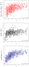 |
Fig. 1. Specific BHAR (upper panel), host galaxy stellar mass (middle panel), and SFR (lower panel) as a function of spectroscopic redshifts for 884 CCL Type 2 AGN with known spectrospic redshifts. |
We then made subsamples in bins of galaxy stellar mass, specific BHAR, and SFR. Specifically, to avoid selection effects between the different bins of stellar mass (see Powell et al. 2018) we defined two bins of Mstar and then for each bin, we randomly selected N AGN of the sample, with N the larger number of sources in the bin, to match the distributions in redshift, λBHAR and SFR. Similarly, we defined two bins in specific BHAR (SFR) and randomly selected subsamples with similar redshift, stellar mass, and SFR (λBHAR) distributions. The final subsamples consist of (a) 362 low and 374 high galaxy stellar mass AGN using a cut at log (Mstar/M⊙) = 10.7 (see Fig. 2); (b) 339 low and 326 high specific BHAR AGN with a cut at log (λBHAR/[erg s−1
 ]) = 32.6 (see Fig. 3); and (c) 262 low and 247 high SFR AGN cutting at log (SFR/Mstar yr−1) = 1.4 (see Fig. 4). The characteristics of these subsamples are summarized in Table 1.
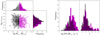 |
Fig. 2. Host galaxy stellar mass as a function of specific BHAR (left panel) for low (log Mstar/[M⊙] ≲ 10.75) and high (> 10.75) stellar mass subsamples. The corresponding distribution in terms of Mstar, λBHAR, SFR, and spectroscopic redshift (right panel) are shown for the two AGN subsets. |
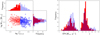 |
Fig. 3. Specific BHAR as a function of host galaxy stellar mass (left panel) for low (log λBHAR ≲ 32.6) and high (> 32.6) specific BHAR subsamples. The corresponding distribution in terms of Mstar, λBHAR, SFR, and spectroscopic redshift (right panel) are shown for the two AGN subsets. |
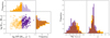 |
Fig. 4. Star formation rate as a function of host galaxy stellar mass (left panel) for low (log SFR ≲ 1.4) and high (> 1.4) SFR subsamples. The corresponding distribution in terms of Mstar, λsBHAR, SFR, and spectroscopic redshift (right panel) are shown for the two subsets. |
Properties of the AGN samples.
3. Projected 2pcf
The most commonly used quantitative measure of large-scale structure is the 2pcf, ξ(r), which traces the amplitude of AGN clustering as a function of scale. The quantity ξ(r) is defined as a measure of the excess probability dP, above what is expected for an unclustered random Poisson distribution, of finding an AGN in a volume element dV at a separation r from another AGN,
![Mathematical equation: $$ \begin{aligned} \mathrm{d}P = n[1 + \xi (r)]\mathrm{d}V, \end{aligned} $$](/articles/aa/full_html/2019/12/aa36191-19/aa36191-19-eq16.gif) (2)
(2)
where n is the mean number density of the AGN sample (Peebles 1980). Measurements of ξ(r) are generally performed in comoving space, where r is measured in units of h−1 Mpc.
We measured the projected 2pcf in bins of rp and π (distances perpendicular and parallel to the line of sight, respectively) using CosmoBolognaLib, a large set of Open Source C++ numerical libraries for cosmological calculations (Marulli et al. 2016), which counts the number of pairs of galaxies in a catalog separated by rp and π. We then integrated along the π-direction to eliminate any redshift-space distorsion. and we estimated the so-called projected correlation function wp(rp) (Davis & Peebles 1983) as
 (3)
(3)
where ξ(rp, π) is the two-point correlation function in terms of rp and π, measured using the Landy & Szalay (1993, LS) estimator
![Mathematical equation: $$ \begin{aligned} \xi = \frac{1}{\mathrm{RR}^{\prime }} [\mathrm{DD}^{\prime }-2\mathrm{DR}^{\prime }+ \mathrm{RR}^{\prime }], \end{aligned} $$](/articles/aa/full_html/2019/12/aa36191-19/aa36191-19-eq18.gif) (4)
(4)
where DD′, DR′, and RR′ are the normalized data-data, data-random, and random-random pairs.
The measurements of the 2pcf requires the construction of a random catalog with the same selection criteria and observational effects as the data. To this end, we constructed a random catalog in which each simulated source is placed at a random position in the sky, with its flux randomly extracted from the catalog of real source fluxes. The simulated source is kept in the random sample if its flux is above the sensitivity map value at that position (Miyaji et al. 2007; Cappelluti et al. 2009). The corresponding redshift for each random object is then assigned based on the smoothed redshift distribution of the AGN sample.
The value of πmax is chosen such that the amplitude of the projected 2pcf converges and gets noisier for any higher values. We calculated the covariance matrix via the jackknife resampling method as follows:
![Mathematical equation: $$ \begin{aligned} C_{i,j} =&\frac{M}{M-1} \sum _{k}^{M} \left[ w_k (r_{\mathrm{p},i}) - \langle w(r_{\mathrm{p},i}) \rangle \right] \nonumber \\&\times \left[w_k(r_{\mathrm{p},j}) - \langle w(r_{\mathrm{p},j}) \rangle \right], \end{aligned} $$](/articles/aa/full_html/2019/12/aa36191-19/aa36191-19-eq19.gif) (5)
(5)
where we split the sample into M = 9 sections of the sky, and computed the cross-correlation function when excluding each section (wk). We quote the errors on our measurement as the square root of the diagonals,  .
.
In the halo model approach, the large-scale amplitude signal is due to the correlation between objects in distinct halos and the bias parameter defines the relation between the large-scale clustering amplitude of the AGN correlation function and the DM two-halo term as follows:
 (6)
(6)
We first estimated the DM two-halo term at the median redshift of the sample, using
 (7)
(7)
where
![Mathematical equation: $$ \begin{aligned} \xi ^{2-h}_{\rm DM}(r)=\frac{1}{2\pi ^2}\int P^{2-h}(k)k^2 \left[\frac{\sin (kr)}{kr} \right] \mathrm{d}k. \end{aligned} $$](/articles/aa/full_html/2019/12/aa36191-19/aa36191-19-eq23.gif) (8)
(8)
The expression P2 − h(k) is the Fourier transform of the linear power spectrum. In particular, we based our estimation of the linear power spectrum on Eisenstein & Hu (1999), which is also implemented in CosmoBolognaLib.
4. Results
4.1. Large-scale bias versus Mstar
The goal of this paper is to study the AGN clustering dependence on host galaxy stellar mass, specific BHAR and SFR. In this section, we focus on the clustering properties of CCL Type 2 AGN as a function of host stellar mass Mstar.
As shown in Fig. 5 (upper panel), the projected 2pcf wp(rp) of 362 (374) AGN with log (Mstar/M⊙) < 10.7 (≳10.7) was measured in the rp range 1−30 h−1 Mpc, following Eq. (3). The typical value of πmax used in clustering measurements of both optically selected luminous quasars and X-ray selected AGN is ∼20−100 h−1 Mpc (e.g., Zehavi et al. 2005; Coil et al. 2009; Krumpe et al. 2010; Allevato et al. 2011). We found the optimal πmax value to be = 60 h−1 Mpc, by deriving the value at which the amplitude of the signal appears to level off.
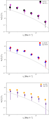 |
Fig. 5. Projected 2pcf of CCL COSMOS Type 2 AGN as a function of panel a: host galaxy stellar mass, log Mstar < 10.7 (black squares), and ≳10.7 (magenta triangles); panel b: specific BHAR, logλBHAR < 32.6 (red circles), and ≳32.6 (blue triangles); panel c: log SFR < 1.4 (orange pentagons) and ≳1.4 (purple stars). The gray line shows the DM projected 2pcf at mean z ∼ 1. |
The 1σ errors on wp(rp) are the square root of the diagonal components of the covariance matrix (Miyaji et al. 2007; Krumpe et al. 2010; Allevato et al. 2016) estimated using the jackknife method. The latter quantifies the level of correlation between different bins.
Following Eq. (6), we derived the best-fit bias using a χ2 minimization technique with one free parameter χ2 =  . In detail, Δ is a vector composed of wp(wp) – wmod(rp), ΔT is its transpose, and
  is the inverse of covariance matrix. The latter full covariance matrix is used in the fit to take into account the correlation between errors.
As shown in Table 1, we derived for the low and high Mstar subsamples b = 2.14 and b = 2.31
 at mean z ∼ 1, respectively. Following the bias–mass relation b(Mh, z) described in van den Bosch (2002) and Sheth et al. (2001), the large-scale bias values correspond to typical masses of the hosting halos of log(Mh/M⊙ h−1) = 12.93
 and 13.03
 , for the low and high stellar mass subsamples, respectively. It is worth noting that these two AGN subsets have similar distributions in terms of specific BHAR, SFR, and redshift. Throughout this work, we refer to typical halo mass as the DM halo mass that satisfies b = b(Mhalo) (e.g., Hickox 2009; Allevato et al. 2014, 2016; Mountrichas et al. 2019).
4.2. AGN bias versus λBHAR and SFR
In this section we investigate the clustering dependence of CCL Type 2 COSMOS AGN on specific BHAR and SFR. For this purpose, we estimated the projected 2pcf of 300 low and 306 high specific BHAR AGN using a cut at log (λBHAR erg−1 s ) = 32.6 (Fig. 5, middle panel) and (b) 251 low and 260 high SFR AGN cutting at log (SFR/Mstar yr−1) = 1.4 (Fig. 5, lower panel).
In detail, we found a large-scale bias b = 2.32 and b = 2.40
 for the low and high λBHAR, respectively. These results suggest no bias evolution with specific BHAR, with a corresponding typical mass of the hosting halos of log(Mh/M⊙ h−1) = 13.02
 and 13.11
 , respectively. On the contrary, AGN with low SFR are more clustered and reside in more massive dark matter halos (log Mh/M⊙ h−1 = 13.14
 compared to high SFR objects (log Mh/M⊙ h−1 = 12.94
 ).
).
5. Discussion
5.1. Clustering dependence on stellar mass
We have performed clustering measurements as a function of host galaxy stellar mass, specific BHAR, and SFR using CCL Type 2 AGN at mean z ∼ 1. In particular, our results suggest a constant bias evolution as a function of Mstar for Type 2 AGN in the particular stellar mass and redshift range investigated in this work (Fig. 6).
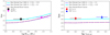 |
Fig. 6. Large-scale bias evolution as a function of host galaxy stellar mass (left panel) and specific BHAR (right panel) for CCL Type 2 AGN and mock AGN. These are matched to have the same host galaxy properties of CCL Type 2 AGN, for Q = 1 and = 2 (according to the legend), which correspond to a relative fraction of satellite AGN |

As shown in Fig. 7, our results are in agreement with the Mstar − Mh relation found in Viitanen et al. (2019) for XMM-COSMOS AGN at similar redshift. It is worth noting that although our study includes XMM-COSMOS AGN, we only focused on Type 2 AGN. Moreover, our larger CCL COSMOS catalog allows us to split the sample according to the galaxy stellar mass while having matched SFR, specific BH accretion rate, and z distributions.
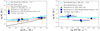 |
Fig. 7. Galaxy stellar mass as a function of dark matter halo mass as derived for CCL Type 2 AGN (dark blue circles) at mean z ∼ 1, XMM-COSMOS AGN (orange stars) at z ∼ 1 (low Mstar) and ∼1.4 (high Mstar) in Viitanen et al. (2019), XMM-XXL AGN (green triangles), and matched normal galaxies (blue squares) in Mountrichas et al. (2019) at mean z ∼ 0.8. The error bars on x-axis represent typical measurement error on the stellar mass estimates of each subsample. The Mstar − Mh and Mstar–SFR relations for matched mock AGN (continuous gray line) and mock matched normal galaxies (dotted red line) are shown. For comparison, the halo-stellar mass relation is shown for the full sample of mock galaxies as a dashed black line. |
Our results are also in agreement with Mountrichas et al. (2019), albeit they inferred a slightly steeper Mstar − Mh relation at mean z ∼ 0.8. In detail, they found that high stellar mass XMM-XXL AGN (both Type 1 and Type 2 sources) resides in slightly more massive halos than low stellar mass objects, when applying a cut at log (Mstar/M⊙) = 10.8 (10.7 in our work). They also showed that the same Mstar–Mh relation is observed for a matched sample of normal non-active galaxies.
The relation between galaxies and their hosting halos has been derived for normal galaxies in different clustering studies (Zheng et al. 2007; Wake et al. 2008; Mostek et al. 2013; Coil et al. 2007) at similar (z ∼ 1) and higher redshift (Bielby et al. 2013; Legrand et al. 2018). These results suggest a more steeper Mstar–Mh relation for non-active galaxies than found for CCL Type 2 AGN and from previous clustering measurements of AGN and for matched normal galaxies.
5.2. Clustering dependence on λBHAR and SFR
We found a constant typical dark matter halo mass as a function of specific BHAR, λBHAR. The same trend has been observed at similar redshift for XMM-COSMOS AGN by Viitanen et al. (2019) and at lower redshift (0.2 < z < 1.2) by Mendez et al. (2016), using PRIMUS and DEEP2 redshift surveys. Assuming a bolometric correction, the specific BHAR can be considered as a proxy of the Eddington ratio (Eq. (1)). Krumpe et al. (2015) found no statistically significant clustering dependence on λEdd for RASS Type 1 AGN at 0.16 < z < 0.36. Our results suggest the same constant bias evolution with Eddington ratio for both RASS Type 1 and COSMOS Type 2 AGN at different redshifts.
On the contrary, we found a negative bias dependence on SFR (see Fig. 7), with lower SFR AGN more clustered than higher SFR objects. This clustering result suggests that splitting the sample according to SFR leads to larger hosting halo mass being associated with lower SFR AGN; i.e., given the same galaxy stellar mass distribution, AGN in low SFR galaxies reside in more massive halos than AGN in high SFR hosts.
Clustering analysis of AGN as a function of host galaxy SFR has been performed by Mountrichas et al. (2019) for X-ray selected XMM-XXL AGN at z = [0.5−1.2]. In particular, they split the AGN sample using a cut at log (SFR/Mstar yr−1) = 1.1 (1.4 in our study) and derived typical halo masses of log (Mh/M⊙ h−1) = 13.08 and 12.54
 at z ∼ 0.8, for the low and high SFR subsets, respectively. These results agree very well with our findings for CCL Type 2 AGN at higher redshift, suggesting a negative clustering dependence as a function of SFR.
A similar trend has been observed for normal non-active galaxies in different studies. Mostek et al. (2013) studied stellar mass-limited samples of DEEP2 galaxies and found that the clustering amplitude increases with decreasing SFR. Similarly, Coil et al. (2007) suggested a strong evolution of the large-scale bias with SFR (and sSFR) in PRIMUS and DEEP2 surveys.
Our measured SFR–Mh relation agrees with the environment quenching picture, where most galaxies in clusters are passive, regardless of their mass (e.g., Peng et al. 2010a,b, 2012). In particular, the passive fraction in both central and satellite galaxies strongly correlates with the halo mass at fixed stellar mass. Above a characteristic halo mass (∼1012M⊙) cooling times are long, and the gas that accretes onto the galaxy is hot, so star formation is inefficient (e.g., Gabor & Dave 2015; Birnboim & Dekel 2003, see also Peng et al. 2015, for observational evidence for quenching via gas exhaustion, or “strangulation”). However, CCL Type 2 AGN also cover the redshift range in which a difference in galaxy SFR properties with environments is ceasing (e.g., George et al. 2013; Erfanianfar et al. 2016 at z ≲ 1.2); the main difference is the fraction of bulge-dominated galaxies as a function of halo mass. Then the SFR cut might also lead to higher weight of bulge-dominated galaxies, which reside in more massive halos.
5.3. Comparison with AGN mock catalogs
5.3.1. Methodology
Several semi-analytical models and hydrodynamical simulations (e.g., Springel et al. 2005; Hopkins et al. 2006; Menci et al. 2008) have been developed in recent years to describe the main mechanisms that fuel the central BHs. With suitable adjustment of parameters, these models can explain many aspects of AGN phenomenology (e.g., Hopkins et al. 2006, 2008). However, our scant knowledge of the key processes imposes a heavy parameterization of the physics regulating the cooling, star formation, feedback, and merging of baryons. Thus, current models present serious degeneracies, i.e., they reproduce similar observables by invoking very different scenarios (Lapi & Cavaliere 2011). Instead, in semiempirical models (SEMs) variables such as galaxy stellar mass, BH mass, and AGN luminosity are assigned through a combination of observational and theoretical scaling relations. These SEMs represent an original and competitive methodology, which is fast, flexible and relies on just a few input assumptions. Mock catalogs of galaxies and their BHs can be created via semiempirical relations starting from large samples of dark matter halos extracted from N-body simulations. Therefore, AGN mock catalogs effectively provide a complementary approach to more complex models of AGN and galaxy evolution (e.g., Conray & White 2013), which can be directly compared with current and future clustering measurements. The SEM for the large-scale distribution of AGN has been used to make realistic predictions for the clustering signal in future experiments and test observational selection effects and biases (e.g., Georgakakis et al. 2018; Comparat et al. 2019).
In this study, we compared our observational results in COSMOS with mock catalogs of active and non-active galaxies created via SEMs based on large N-body simulations. The full description of numerical routines to create mock catalogs of galaxies and their BHs using SEMs is given in Allevato et al. (in prep.). In this work we only describe the important steps in the generation of the AGN mock catalogs and we refer to Allevato et al. for more details. First, we extracted a large catalog of dark matter halos and subhalos from MultiDark1-Planck 2 (MDPL2; Riebe et al. 2013) at the redshift of interest, which currently provides the largest publicly available set of high-resolution and large volume N-body simulations (box size of 1000 h−1 Mpc, mass resolution of 1.51 × 10⁹ h−1M⊙). The ROCKSTAR halo finder (Behroozi et al. 2013) has been applied to the MDPL2 simulations to identify halos and flag those (sub-halos) that lie within the virial radius of a more massive host halo. The mass of the dark matter halo is defined as the virial mass in the case of host halos and the infall progenitor virial mass for sub-halos. In the analysis that follows, we use the simulation snapshot at z = 1, which corresponds to the mean redshift of our AGN clustering measurements.
We assign to each halo: (a) a galaxy stellar mass deduced from the Grylls et al. (2019) semiempirical relation, inclusive of intrinsic (0.15 dex) and measurement scatter (0.2 dex for stellar mass estimates in our COSMOS sample). Satellites are assigned a stellar mass at the redshift of infall; (b) a BH mass assuming empirical BH-galaxy mass relation derived in Shankar et al. (2016), inclusive of a stellar mass dependent scatter; (c) an X-ray luminosity following the observationally deduced specific BHAR distribution described by a Schechter function as suggested in Bongiorno et al. (2012, 2016), Aird et al. (2012), and Georgakakis et al. (2017); (d) a SFR following the SFR – stellar mass relation described in Tomczak et al. (2016) for main sequence galaxies, including intrinsic (0.2 dex) and measurement (0.2 dex for our COSMOS sample) scatter; (e) a hydrogen column density NH assigned following the Ueda et al. (2014) empirical distribution such that AGN can be classified into Type 2 obscured, Type 1 unobscured, and Compton thick AGN; and (f) a duty cycle, i.e., a probability for each BH of being active, following Schulze et al. (2015).
The main difference between our approach and recent studies based on SEMs (e.g., Georgakakis et al. 2019; Comparat et al. 2019) is that the latter assign an Eddington ratio to each mock BH, and consider active the objects with a specific BHAR above a given value. On the contrary, we assigned to each BH an Eddington ratio combined with a probability of being active, which depends on the BH mass. A comparison between the different SEMs is beyond the scope of this paper and is discussed in Allevato et al. (in prep.).
We then selected a sample of mock AGN, matched to have the same galaxy stellar mass, specific BHAR, SFR, and X-ray luminosity distributions of CCL Type 2 AGN, including only Type 2 objects selected according to NH values. This corresponds to mock AGN living in dark matter halos (parent halos for satellite galaxies) with log Mh[M⊙] > 12. To each parent halo mass Mhalo, a bias is assigned that satisfies b = b(Mhalo), following the same bias-mass relation used for CCL Type 2 AGN (van den Bosch 2002; Sheth et al. 2001). Similarly, we selected a sample of normal non-active galaxies with the same galaxy stellar mass, SFR, and X-ray luminosity distributions of CCL Type 2 AGN.
5.3.2. Bias for mock AGN
We follow the formalism of Shankar et al. (2019) to derive the bias of mock AGN and normal galaxies as a function of galaxy stellar mass, specific BHAR, and SFR using the relative probabilities of central and satellite galaxies of being active Q = Us/Uc.
The bias of mock objects with stellar mass in the range Mstar and Mstar + dMstar is estimated as
![Mathematical equation: $$ \begin{aligned} b(M_{\rm star}) = \frac{1}{N_{\rm bin}} \sum _{i=1}^{N_{\rm bin}} b[M_{\mathrm{h},i} (M_{\rm star})], \end{aligned} $$](/articles/aa/full_html/2019/12/aa36191-19/aa36191-19-eq40.gif) (9)
(9)
where for each bin of stellar mass the sum runs over all host parent halos. If the probabilities for galaxies to be active, i.e., the AGN duty cycle U(Mstar) = [Uc(Mstar)Nc(Mstar)+Us(Mstar)Ns(Mstar)]/N(Mstar) is included, the generalized formula is written as
![Mathematical equation: $$ \begin{aligned} b = \frac{\left[\sum _{i=1}^{N_{\rm c}} U_{\mathrm{c},i}(M_{\rm star}) b_{\mathrm{c},i}(M_{\rm star}) + \sum _{i=1}^{N_{\rm s}} U_{\mathrm{s},i}(M_{\rm star}) b_{\mathrm{sat},i}(M_{\rm star})\right]}{\left[\sum _{i=1}^{N_{\rm cen}} U_{\mathrm{c},i}(M_{\rm star})+ \sum _{i=1}^{N_{\rm s}} U_{\mathrm{s},i}(M_{\rm star}) \right]}, \end{aligned} $$](/articles/aa/full_html/2019/12/aa36191-19/aa36191-19-eq41.gif) (10)
(10)
where Uc(Mstar) = U(Mstar)N(Mstar)/[(Nc(Mstar)+QNs(Mstar)] is the duty cycle of central AGN, Us(Mstar)=QUc(Mstar) is the duty cycle of satellite AGN, and N(Mstar) = Nc(Mstar)+Ns(Mstar) is the number of central and satellite galaxies in the stellar mass bin Mstar and Mstar + dMstar.
When Us = Uc, i.e., if all central and satellite galaxies are active or share equal probabilities of being active, Eq. (10) reduces to Eq. (9). It is important to note that the bias is thus mainly affected by Q and then by the fraction of AGN in satellite halos  , so that
 ![Mathematical equation: $ Q = f_{\mathrm{sat}}^{\mathrm{AGN}} (1-f_{\mathrm{sat}}^{\mathrm{BH}}) / [({1-f_{\mathrm{sat}}^{\mathrm{AGN}}})f_{\mathrm{sat}}^{\mathrm{BH}}] $](/articles/aa/full_html/2019/12/aa36191-19/aa36191-19-eq43.gif) , where
, where  is the total fraction of (active and non-active) BHs in satellites with host galaxy stellar mass within Mstar and Mstar + dMstar. In our mock of AGN matched to CCL Type 2 AGN, we have a total fraction of satellite galaxies
  , which corresponds to Q = 1 for a fraction of satellite AGN
  ∼ 0.1 and Q = 2 for
  ∼ 0.15, respectively. Similarly, Eq. (10) can be written in bins of specific BHAR and SFR, for Q = 1 and 2, respectively.
5.3.3. Predictions from SEMs
Figure 6 shows the mean bias as a function of the host galaxy stellar mass and specific BHAR for mock AGN (Eq. (10)) and for normal galaxies (Eq. (9)), where Q = 1 and = 2, which corresponds to a fraction of satellite AGN  and ∼0.15, respectively. The host galaxy stellar masses in the mock catalog are assigned by following Grylls et al. (2019), i.e., are defined as Sersic + exponential model (Bernardi et al. 2013) with a mass-to-light ratio from Bell et al. (2013). To correct for the different definition in COSMOS (Bruzual & Charlot 2003; Chabrier 2003) we need to decrease the stellar masses of mock objects by a factor of ∼0.15 dex (Grylls et al. 2020).
The bias–Mstar relation for mock AGN and matched mock normal galaxies is slightly steeper compared to clustering measurements of COSMOS AGN, when we assume the same probability of satellite and central galaxies of being active (Q = 1). In particular, we found that CCL Type 2 AGN host galaxies with low Mstar reside in slightly more massive halos than mock AGN and normal galaxies of similar stellar mass. It is important to note that when Q = 1, Eq. (10) reduces to the simple case of Eq. (9), and AGN and normal galaxies have the same bias–Mstar relation.
Our results for CCL Type 2 AGN can be reproduced if we assume a larger satellite AGN fraction  and Q ∼ 2. For instance, Leauthaud et al. (2015) found
  for COSMOS AGN at z ≲ 1. The importance of the relative fraction of satellite AGN has also been underlined in Viitanen et al. (2019). They have suggested that when excluding AGN that are associated with galaxy groups, the bias of low Mstar objects decreases, while not affecting the high stellar mass systems. Similar results are found in Mountrichas et al. (2013) for moderate luminosity X-ray AGN at z ∼ 1. This is because at lower stellar mass, AGN are more likely in satellite galaxies hosted by more biased and massive parent dark matter halos. Similarly, the bias as a function of specific BHAR and SFR of CCL Type 2 AGN is better reproduced by mock AGN with Q = 2. It is worth noting that the bias–Mstar, bias–λEdd and bias–SFR relations of normal non-active mock galaxies are independent of the relative duty cycle of AGN in satellite and central halos, Q.
Our results thus suggest that for CCL Type 2 AGN at z ∼ 1, the relative probabilities of AGN in satellites is roughly two times larger than in central halos; the fraction of AGN in satellite halos is consistent with  . Starikova et al. (2015) studied the HOD of AGN detected by the Chandra X-Ray Observatory in the Bootes field over a redshift interval z = [0.17−3], showing a satellite fraction of ∼10%. Allevato et al. (2012) performed direct measurement of the HOD for COSMOS AGN based on the mass function of galaxy groups hosting AGN and found that the duty cycle of satellite AGN is comparable or even larger than that of central AGN, i.e., Q ≳ 1. The central locations of the quasar host galaxies are expected in major merger models because mergers of equally sized galaxies preferentially occur at the centers of DM halos (Hopkins et al. 2008). Our predictions from mock matched AGN suggests a high percentage of satellite AGN, in agreement with studies that have found a small fraction of AGN associated with morphologically disturbed galaxies (Cisterans et al. 2011; Schawinski et al. 2011; Rosario et al. 2011) and that have suggested secular processes and bar instabilities are efficient in producing luminous AGN (e.g., Georgakakis et al. 2009; Allevato et al. 2011).
Figure 7 shows the typical dark matter halo mass as a function of galaxy stellar mass, as found for CCL Type 2 AGN at mean z ∼ 1, for XMM-XXL AGN at z ∼ 0.8 (Mountrichas et al. 2019, green triangles) and as predicted for matched mock AGN and matched normal galaxies for Q = 2. The predictions from mock AGN well reproduce the observations in COSMOS, as well as the results for XMM-XXL AGN at similar redshift.
A slightly steeper trend is observed for matched normal mock galaxies; non-active BH reside in less massive parent halos than mock AGN with low host galaxy stellar mass. This is in contrast with the results of Mountrichas et al. (2019), at least for low Mstar galaxies. They suggest that AGN have the same stellar-to-halo mass ratio of matched normal galaxies at all stellar masses. Previous clustering studies of normal galaxies (e.g., Zheng et al. 2007; Coil et al. 2007) have suggested a steeper halo – stellar mass relation at similar redshift. A flatter Mstar–Mh relation found for mock matched galaxies is mainly due to the large scatter (measurement 0.2 dex and intrinsic 0.15 dex) in the input relation (see Sect. 4.3.1) used to create the mock catalog to reproduce the stellar mass measurement error in COSMOS, and to the selections in terms of LX, Mstar, specific BHAR, and SFR applied to match CCL Type AGN hosts. Figure 7 shows that when selecting a subsample of galaxies matched to have the same properties of CCL Type 2 AGN hosts, the galaxy bias is driven up at low stellar mass with respect to the full galaxy population.
Figure 7 also shows the halo mass–SFR relation for mock AGN and matched normal galaxies. The predictions are almost consistent with our results in COSMOS and with previous studies in XMM-XXL at similar redshifts (Mountrichas et al. 2019), but suggest a slightly flatter SFR–Mh relation than observed. A constant SFR as a function of the halo mass is a consequence of the almost flat Mstar–Mh relation obtained for mock objects, combined with the input assumption that each mock AGN and galaxy follow a simple main sequence SFR–Mstar relation.
We stress that given the limited sample of CCL Type 2 AGN in bins of Mstar, SFR and specific BHAR, we can only estimate typical halo masses as a function of AGN host galaxy properties, from the modeling of the two-halo term. The full halo mass distribution and halo occupation (possibly separating the contribution of AGN in central and satellite galaxies) require higher statistics to constrain the clustering signal at small scale. Currently, one possibility to overcome the low statistics is to combine available samples of AGN in X-ray surveys, such as CCL (Civano et al. 2016), AEGIS and 4 Ms CDFS (Georgakakis et al. 2014), and XMM-XXL (Mendez et al. 2016), with robust host galaxy property estimates. Following this approach the number of AGN with known spectroscopic redshift can be almost doubled with respect to the sample of Type 2 AGN used in this work. In subsequent years, the synergy of eRosita, 4MOST, WISE, as well as Euclid and JWST in the near future, will allow us to derive host galaxy stellar mass and SFR estimates of millions of moderate-high luminosity AGN up to z ∼ 2.
Moreover, our clustering measurements refer to Type 2 AGN only. New CCL data are now available for Type 1 AGN (Suh et al. 2019) and then AGN clustering dependence on host galaxy properties will be probed in the near future as a function of obscuration.
6. Conclusions
In this paper, we have performed clustering measurements of CCL Type 2 AGN at mean z ∼ 1, to probe the AGN large-scale bias dependence on host galaxy properties, such as galaxy stellar mass, specific BHAR, and SFR. We found no dependence of the AGN large-scale bias on galaxy stellar mass and specific BHAR, suggesting almost flat Mstar–Mh and λBHAR–Mh relations. A negative clustering dependence is instead observed as a function of SFR, with the typical hosting halo mass increasing with decreasing SFR. Mock catalogs of AGN matched to have the same host galaxy properties of CCL Type 2 AGN predict the observed Mstar − Mh, SFR–Mh and λBHAR − Mh relations, when assuming a fraction of satellite AGN  % and then Q = 2. Mock matched normal galaxies follow a slightly steeper Mstar − Mh relation, where low mass mock galaxies reside in slightly less massive halos than mock AGN of similar mass. Similarly, mock galaxies reside in less massive hosting halos than mock AGN with similar specific BHAR and SFR, at least for Q > 1.
Acknowledgments
VA acknowledges funding from the European Union’s Horizon 2020 research and innovation programme under grant agreement No 749348. TM is supported by CONACyT 252531 and UNAM-DGAPA PAPIIT IN111319.
References
- Aird, J., Coil, A. L., Moustakas, J., et al. 2012, ApJ, 746, 90 [NASA ADS] [CrossRef] [Google Scholar]
- Aird, J., Coil, A. L., Georgakakis, A., et al. 2018, MNRAS, 474, 1225 [NASA ADS] [CrossRef] [Google Scholar]
- Allevato, V., Finoguenov, A., Cappelluti, N., et al. 2011, ApJ, 736, 99 [NASA ADS] [CrossRef] [Google Scholar]
- Allevato, V., Finoguenov, A., Hasinger, G., et al. 2012, ApJ, 758, 47 [NASA ADS] [CrossRef] [Google Scholar]
- Allevato, V., Finoguenov, A., Civano, F., et al. 2014, ApJ, 796, 4 [NASA ADS] [CrossRef] [Google Scholar]
- Allevato, V., Civano, F., Finoguenov, A., et al. 2016, ApJ, 832, 70 [NASA ADS] [CrossRef] [Google Scholar]
- Behroozi, P., & Silk, J. 2018, MNRAS, 477, 5382 [NASA ADS] [CrossRef] [Google Scholar]
- Behroozi, P. S., Wechsler, R. H., & Conroy, C. 2013, ApJ, 770, 57 [NASA ADS] [CrossRef] [Google Scholar]
- Bell, E. F., McIntosh, D. H., Katz, N., et al. 2013, ApJS, 149, 289 [Google Scholar]
- Bernardi, M., Meert, A., Sheth, R. K., et al. 2013, MNRAS, 436, 697 [NASA ADS] [CrossRef] [Google Scholar]
- Bielby, R., Hill, M. D., Shanks, T., et al. 2013, MNRAS, 430, 425 [NASA ADS] [CrossRef] [Google Scholar]
- Birnboim, Y., & Dekel, A. 2003, MNRAS, 345, 349 [NASA ADS] [CrossRef] [Google Scholar]
- Bongiorno, A., Merloni, A., Brusa, M., et al. 2012, MNRAS, 427, 3103 [NASA ADS] [CrossRef] [Google Scholar]
- Bongiorno, A., Schultze, A., Merloni, A., et al. 2016, A&A, 588, A78 [NASA ADS] [CrossRef] [EDP Sciences] [Google Scholar]
- Bruzual, G., & Charlot, S. 2003, MNRAS, 344, 1000 [NASA ADS] [CrossRef] [Google Scholar]
- Cappelluti, N., Brusa, M., Hasinger, G., et al. 2009, A&A, 497, 635 [NASA ADS] [CrossRef] [EDP Sciences] [Google Scholar]
- Cappelluti, N., Aiello, M., Burlon, D., et al. 2010, ApJ, 716, 209 [NASA ADS] [CrossRef] [Google Scholar]
- Civano, F., Marchesi, S., Comastri, A., et al. 2016, ApJ, 819, 62 [NASA ADS] [CrossRef] [Google Scholar]
- Cisterans, M., Jahnke, K., Inskip, K. J., et al. 2011, ApJ, 726, 57 [NASA ADS] [CrossRef] [Google Scholar]
- Chabrier, G. 2003, ApJ, 586, L133 [NASA ADS] [CrossRef] [Google Scholar]
- Coil, A. L., Hennawi, J. F., Newman, J. A., et al. 2007, ApJ, 654, 115 [NASA ADS] [CrossRef] [Google Scholar]
- Coil, A. L., Georgakakis, A., Newman, J. A., et al. 2009, ApJ, 701, 1484 [NASA ADS] [CrossRef] [Google Scholar]
- Coil, A. L., Mendez, A. J., Eisenstein, D. J., & Moustakas, J. 2017, ApJ, 838, 87 [NASA ADS] [CrossRef] [Google Scholar]
- Comparat, J., Merloni, A., Salvato, M., et al. 2019, MNRAS, 487, 2005 [NASA ADS] [CrossRef] [Google Scholar]
- Conray, C., & White, M. 2013, ApJ, 762, 70 [NASA ADS] [CrossRef] [Google Scholar]
- Coupon, J., Arnouts, S., van Waerbeke, L., et al. 2015, MNRAS, 449, 1352 [NASA ADS] [CrossRef] [Google Scholar]
- Croom, S. M., Boyle, B. J., Shanks, T., et al. 2005, MNRAS, 356, 415 [NASA ADS] [CrossRef] [Google Scholar]
- Davis, M., & Peebles, P. J. E. 1983, ApJ, 267, 465 [NASA ADS] [CrossRef] [Google Scholar]
- Eisenstein, D. J., & Hu, W. 1999, ApJ, 511, 5 [NASA ADS] [CrossRef] [Google Scholar]
- Elvis, M., Civano, F., Vignani, C., et al. 2009, ApJS, 184, 158 [NASA ADS] [CrossRef] [Google Scholar]
- Erfanianfar, G., Popesso, P., Finoguenov, A., et al. 2016, MNRAS, 455, 2839 [NASA ADS] [CrossRef] [Google Scholar]
- Gabor, J. M., & Dave, R. 2015, MNRAS, 447, 374 [NASA ADS] [CrossRef] [Google Scholar]
- Georgakakis, A., Coil, A. L., Laird, E. S., et al. 2009, MNRAS, 397, 623 [NASA ADS] [CrossRef] [Google Scholar]
- Georgakakis, A., Mountrichas, G., Salvato, M., et al. 2014, MNRAS, 443, 3327 [NASA ADS] [CrossRef] [Google Scholar]
- Georgakakis, A., Aird, J., Schulze, A., et al. 2017, MNRAS, 471, 1976 [NASA ADS] [CrossRef] [Google Scholar]
- Georgakakis, A., Comparat, J., Merloni, A., et al. 2018, MNRAS, 487, 275 [NASA ADS] [CrossRef] [Google Scholar]
- Georgakakis, A., Comparat, J., Merloni, A. et al. 2019, MNRAS, 487, 275G [Google Scholar]
- George, M. R., Ma, C. P., Bundy, K., et al. 2013, ApJ, 770, 113 [NASA ADS] [CrossRef] [Google Scholar]
- Grylls, P. J., Shankar, F., Zanisi, L., & Bernardi, M. 2019, MNRAS, 483, 2506 [NASA ADS] [CrossRef] [Google Scholar]
- Grylls, P. J., Shankar, F., Leja, J., et al. 2020, MNRAS, 491, 634 [NASA ADS] [Google Scholar]
- Haring, N., & Rix, H. 2004, ApJ, 604, L89 [NASA ADS] [CrossRef] [Google Scholar]
- Hopkins, P. F., Hernquist, L. C., Thomas, J., et al. 2006, ApJS, 163, 1 [Google Scholar]
- Hopkins, P. F., Hernquist, L. C., Thomas, J., et al. 2008, ApJ, 679, 156 [NASA ADS] [CrossRef] [Google Scholar]
- Hickox, R. C., Jones, C., Forman, W. R., et al. 2009, ApJ, 696, 891 [Google Scholar]
- Koutoulidis, L., Plionis, M., Georgantopoulos, I., & Fanidakis, N. 2013, MNRAS, 428, 1382 [NASA ADS] [CrossRef] [Google Scholar]
- Krumpe, M., Miyaji, T., & Coil, A. L. 2010, ApJ, 713, 558 [NASA ADS] [CrossRef] [Google Scholar]
- Krumpe, M., Miyaji, T., Coil, A. L., & Aceves, H. 2012, ApJ, 746, 1 [NASA ADS] [CrossRef] [Google Scholar]
- Krumpe, M., Miyaji, T., Husemann, B., et al. 2015, ApJ, 815, 21 [NASA ADS] [CrossRef] [Google Scholar]
- Landy, S. D., & Szalay, A. S. 1993, ApJ, 412, 64 [NASA ADS] [CrossRef] [Google Scholar]
- Lapi, A., & Cavaliere, A. 2011, ApJ, 743, 127L [NASA ADS] [CrossRef] [Google Scholar]
- Leauthaud, A., Finoguenov, A., Kneib, J. P., et al. 2010, ApJ, 709, 97 [NASA ADS] [CrossRef] [Google Scholar]
- Leauthaud, A. J., Benson, A., & Civano, F. 2015, MNRAS, 446, 1874 [NASA ADS] [CrossRef] [Google Scholar]
- Legrand, L., McCracken, H. J., Davidzon, I., et al. 2018, MNRAS, 486, 5468 [Google Scholar]
- Magorrian, J., Tremaine, S., Richstone, D., et al. 1998, AJ, 115, 2285 [NASA ADS] [CrossRef] [Google Scholar]
- Marchesi, S., Civano, F., Elvis, M., et al. 2016, ApJ, 817, 34 [NASA ADS] [CrossRef] [Google Scholar]
- Marulli, F., Veropalumbo, A., & Moresco, M. 2016, Astron. Comput., 14, 35 [NASA ADS] [CrossRef] [Google Scholar]
- Menci, N., Fiore, F., Puccetti, S. et al. 2008, ApJ, 686, 219 [NASA ADS] [CrossRef] [Google Scholar]
- Mendez, A. J., Coil, A. L., Aird, J., et al. 2016, ApJ, 821, 55 [NASA ADS] [CrossRef] [Google Scholar]
- Meneux, B., Guzzo, L., de la Torre, S., et al. 2009, A&A, 505, 463 [NASA ADS] [CrossRef] [EDP Sciences] [Google Scholar]
- Miyaji, T., Zamorani, G., Cappelluti, N., et al. 2007, ApJS, 172, 396 [NASA ADS] [CrossRef] [Google Scholar]
- Mostek, N., Coil, A. L., Cooper, M., et al. 2013, ApJ, 767, 89 [NASA ADS] [CrossRef] [Google Scholar]
- Moster, B. P., Naab, T., & White, S. D. M. 2013, MNRAS, 428, 3121 [NASA ADS] [CrossRef] [Google Scholar]
- Moster, B. P., Naab, T., & White, S. D. M. 2018, MNRAS, 477, 1822 [NASA ADS] [CrossRef] [Google Scholar]
- Mountrichas, G., Georgakakis, A., Finoguenov, A., et al. 2013, MNRAS, 430, 661 [NASA ADS] [CrossRef] [Google Scholar]
- Mountrichas, G., Georgakakis, A., & Georgantopoulos, I. 2019, MNRAS, 483, 1374 [NASA ADS] [CrossRef] [Google Scholar]
- Peebles, P. J. E. 1980, The Large Scale Structure of the Universe (Princeton: Princeton Univ. Press) [Google Scholar]
- Peng, Y., Lilly, S. J., Kovač, K., et al. 2010a, ApJ, 721, 193 [NASA ADS] [CrossRef] [Google Scholar]
- Peng, Y., Lilly, S. J., Renzini, A., et al. 2010b, ApJ, 757, 4 [Google Scholar]
- Peng, Y., Lilly, S. J., Renzini, A., et al. 2012, ApJ, 757, 4 [NASA ADS] [CrossRef] [Google Scholar]
- Peng, Y., Maiolino, R., & Cochrane, R. 2015, Nature, 521, 192 [NASA ADS] [CrossRef] [Google Scholar]
- Plionis, M., et al. 2018, A&A, 371, 1824 [Google Scholar]
- Porciani, C., & Norberg, P. 2006, MNRAS, 371, 1824 [NASA ADS] [CrossRef] [Google Scholar]
- Powell, M. C., Cappelluti, N., Urry, C. M., et al. 2018, ApJ, 858, 110 [NASA ADS] [CrossRef] [Google Scholar]
- Riebe, K., Partl, A. M., Enke, H., et al. 2013, AN, 334, 691 [NASA ADS] [Google Scholar]
- Rosario, D. J., McGurk, R. C., Max, C. E., et al. 2011, ApJ, 739, 44 [NASA ADS] [CrossRef] [Google Scholar]
- Ross, N. P., Shen, Y., Strauss, M. A., et al. 2009, ApJ, 697, 1634 [NASA ADS] [CrossRef] [Google Scholar]
- Schawinski, K., Treister, E., Urry, C. M., et al. 2011, ApJ, 727, 31 [NASA ADS] [CrossRef] [Google Scholar]
- Schulze, A., Bongiorno, A., Gavignaud, I., et al. 2015, MNRAS, 447, 2085 [NASA ADS] [CrossRef] [Google Scholar]
- Shankar, F., Bernardi, M., Sheth, R. K., et al. 2016, MNRAS, 460, 3119 [NASA ADS] [CrossRef] [Google Scholar]
- Shankar, F., Allevato, V., Bernardi, M., et al. 2019, Arxiv e-prints [arXiv:1910.10175] [Google Scholar]
- Shen, Y., McBride, C. K., White, M., et al. 2013, ApJ, 778, 98 [NASA ADS] [CrossRef] [Google Scholar]
- Sheth, R. K., Mo, H. J., & Tormen, G. 2001, MNRAS, 323, 1 [NASA ADS] [CrossRef] [Google Scholar]
- Springel, V., Di Matteo, T., Hernquist, L., et al. 2005, ApJ, 620, L79 [NASA ADS] [CrossRef] [Google Scholar]
- Starikova, S., Cool, R., Eisenstein, D., et al. 2015, ApJ, 741, 15 [NASA ADS] [CrossRef] [Google Scholar]
- Suh, H., Civano, F., Hasinger, G., et al. 2017, ApJ, 841, 102 [NASA ADS] [CrossRef] [Google Scholar]
- Suh, H., Civano, F., Hasinger, G., et al. 2019, ApJ, 872, 168 [NASA ADS] [CrossRef] [Google Scholar]
- Tomczak, A. R., Quadri, R. F., Tran, K. V. H., et al. 2016, ApJ, 817, 118 [NASA ADS] [CrossRef] [Google Scholar]
- Wake, D. A., Croom, S. M., Sadler, E. M., & Johnston, H. M. 2008, MNRAS, 391, 1674 [NASA ADS] [CrossRef] [Google Scholar]
- Ueda, Y., Akiyama, M., Hasinger, G., et al. 2014, ApJ, 786, 104 [NASA ADS] [CrossRef] [Google Scholar]
- van den Bosch, F. C. 2002, MNRAS, 331, 98 [Google Scholar]
- Viitanen, A., Allevato, V., Finoguenov, A., et al. 2019, A&A, 629, A14 [NASA ADS] [CrossRef] [EDP Sciences] [Google Scholar]
- Zehavi, I., Eisenstein, D. J., Nichol, R. C., et al. 2005, ApJ, 621, 22 [NASA ADS] [CrossRef] [Google Scholar]
- Zheng, Z., Coil, A. L., & Zehavi, I. 2007, ApJ, 667, 760 [NASA ADS] [CrossRef] [Google Scholar]
All Tables
All Figures
|
Fig. 1. Specific BHAR (upper panel), host galaxy stellar mass (middle panel), and SFR (lower panel) as a function of spectroscopic redshifts for 884 CCL Type 2 AGN with known spectrospic redshifts. |
| In the text | |
|
Fig. 2. Host galaxy stellar mass as a function of specific BHAR (left panel) for low (log Mstar/[M⊙] ≲ 10.75) and high (> 10.75) stellar mass subsamples. The corresponding distribution in terms of Mstar, λBHAR, SFR, and spectroscopic redshift (right panel) are shown for the two AGN subsets. |
| In the text | |
|
Fig. 3. Specific BHAR as a function of host galaxy stellar mass (left panel) for low (log λBHAR ≲ 32.6) and high (> 32.6) specific BHAR subsamples. The corresponding distribution in terms of Mstar, λBHAR, SFR, and spectroscopic redshift (right panel) are shown for the two AGN subsets. |
| In the text | |
|
Fig. 4. Star formation rate as a function of host galaxy stellar mass (left panel) for low (log SFR ≲ 1.4) and high (> 1.4) SFR subsamples. The corresponding distribution in terms of Mstar, λsBHAR, SFR, and spectroscopic redshift (right panel) are shown for the two subsets. |
| In the text | |
|
Fig. 5. Projected 2pcf of CCL COSMOS Type 2 AGN as a function of panel a: host galaxy stellar mass, log Mstar < 10.7 (black squares), and ≳10.7 (magenta triangles); panel b: specific BHAR, logλBHAR < 32.6 (red circles), and ≳32.6 (blue triangles); panel c: log SFR < 1.4 (orange pentagons) and ≳1.4 (purple stars). The gray line shows the DM projected 2pcf at mean z ∼ 1. |
| In the text | |
|
Fig. 6. Large-scale bias evolution as a function of host galaxy stellar mass (left panel) and specific BHAR (right panel) for CCL Type 2 AGN and mock AGN. These are matched to have the same host galaxy properties of CCL Type 2 AGN, for Q = 1 and = 2 (according to the legend), which correspond to a relative fraction of satellite AGN |
| In the text | |
|
Fig. 7. Galaxy stellar mass as a function of dark matter halo mass as derived for CCL Type 2 AGN (dark blue circles) at mean z ∼ 1, XMM-COSMOS AGN (orange stars) at z ∼ 1 (low Mstar) and ∼1.4 (high Mstar) in Viitanen et al. (2019), XMM-XXL AGN (green triangles), and matched normal galaxies (blue squares) in Mountrichas et al. (2019) at mean z ∼ 0.8. The error bars on x-axis represent typical measurement error on the stellar mass estimates of each subsample. The Mstar − Mh and Mstar–SFR relations for matched mock AGN (continuous gray line) and mock matched normal galaxies (dotted red line) are shown. For comparison, the halo-stellar mass relation is shown for the full sample of mock galaxies as a dashed black line. |
| In the text | |
Current usage metrics show cumulative count of Article Views (full-text article views including HTML views, PDF and ePub downloads, according to the available data) and Abstracts Views on Vision4Press platform.
Data correspond to usage on the plateform after 2015. The current usage metrics is available 48-96 hours after online publication and is updated daily on week days.
Initial download of the metrics may take a while.