| Issue |
A&A
Volume 674, June 2023
|
|
|---|---|---|
| Article Number | A214 | |
| Number of page(s) | 12 | |
| Section | Extragalactic astronomy | |
| DOI | https://doi.org/10.1051/0004-6361/202245320 | |
| Published online | 23 June 2023 | |
Large-scale clustering of buried X-ray AGN: Trends in AGN obscuration and redshift evolution
1
Department of Physics, University of Helsinki, PO Box 64 00014 Helsinki, Finland
e-mail: akke.viitanen@helsinki.fi
2
INAF-Osservatorio astronomico di Capodimonte, Via Moiariello 16, 30131 Naples, Italy
3
Scuola Normale Superiore, Piazza dei Cavalieri 7, 56126 Pisa, Italy
4
School of Physics & Astronomy, University of Southampton, Highfield, Southampton, SO17 1BJ
UK
5
INAF-Osservatorio di Astrofisica e Scienza delle Spazio di Bologna, OAS, Via Gobetti 93/3, 40129 Bologna, Italy
Received:
28
October
2022
Accepted:
4
April
2023
Aims. In order to test active galactic nucleus (AGN) unification and evolutionary models, we measured the AGN clustering properties as a function of AGN obscuration defined in terms of hydrogen column density, NH. In addition to measuring the clustering of unobscured (NH < 1022 cm−2) and moderately obscured (1022 ≤ NH < 1023.5) AGNs, we also targeted highly obscured sources (NH ≥ 1023.5) up to redshifts of z = 3.
Methods. We have compiled one of the largest samples of X-ray-selected AGNs from a total of eight deep XMM/Chandra and multiwavelength surveys. We measured the clustering as a function of both AGN obscuration and redshift using the projected two-point correlation function, wp(rp). We modeled the large-scale clustering signal, measured the AGN bias, b(z, NH), and interpreted it in terms of the typical AGN host dark matter halo, Mhalo(z, NH).
Results. We find no significant dependence of AGN clustering on obscuration, suggesting similar typical masses of the hosting halos as a function of NH. This result matches expectations of AGN unification models, in which AGN obscuration depends mainly on the viewing angle of the obscuring torus. We measured, for the first time, the clustering of highly obscured AGNs and find that these objects reside in halos with typical mass log Mhalo = 12.98−0.22+0.17[h−1 M⊙] (12.28−0.19+0.13) at low z ∼ 0.7 (high z ∼ 1.8) redshifts. We find that irrespective of obscuration, an increase in AGN bias with redshift is slower than the expectation for a constant halo mass and instead follows the growth rate of halos, known as the passive evolution track. This implies that for those AGNs the clustering is mainly driven by the mass growth rate of the hosting halos and galaxies across cosmic time.
Key words: dark matter / galaxies: active / galaxies: evolution / large-scale structure of Universe / quasars: general / surveys
© The Authors 2023
 Open Access article, published by EDP Sciences, under the terms of the Creative Commons Attribution License (https://creativecommons.org/licenses/by/4.0), which permits unrestricted use, distribution, and reproduction in any medium, provided the original work is properly cited.
This article is published in open access under the Subscribe to Open model. Subscribe to A&A to support open access publication.
1. Introduction
Active galactic nucleus (AGN) unified models have been a central pillar of AGN phenomenology for nearly four decades. The model states that the central engines and environments of all AGNs are essentially the same. The black hole (BH) at the galaxy center is surrounded by an accretion disk, and its growth takes place behind a dusty, clumpy, obscuring torus (e.g., Antonucci 1993; Urry & Padovani 1995; Netzer 2015). There is substantial evidence that this orientation-based unification model is broadly applicable to local AGNs, whose nuclear regions can be studied in detail (e.g., Hönig et al. 2013; Tristram et al. 2014). However, it is now recognized that such a model is oversimplified and requires ad hoc adjustments to account for the wide range of AGN obscuration properties seen at different redshifts and luminosities (e.g., Merloni et al. 2014). For example, the increasing fraction of obscured AGNs toward high redshifts seems to indicate that obscuration occurs not just in the torus but also on the scale of the host galaxy (La Franca et al. 2005; Ballantyne et al. 2006; Gilli et al. 2022), and that it may be related to the overall galaxy evolution (Treister & Urry 2006; Hasinger 2008; Ueda et al. 2014; Buchner et al. 2015).
Type 1 and 2 AGNs are postulated to be intrinsically the same objects in orientation-based unification models, with Type 1, or broad-line, AGNs showing broad emission lines (full width at half maximum > 1000 km s−1) and Type 2, or narrow-line, AGNs lacking these broad emission features in their optical spectra. Historically, Type 2 AGNs have been described as an obscured version of Type 1 AGNs, with the broad-line-emitting region being hidden behind the partially opaque torus.
An additional way to classify AGNs based on obscuration properties is by using the neutral gas column density, NH, along the line of sight, as derived by X-ray spectral analysis or from the hardness ratio (HR), which is defined from X-ray counts in hard (H) and soft (S) bands as HR = (H − S)/(H + S). Following this approach, AGNs are classified as unobscured (NH < 1022 cm−2), obscured (1022 < NH < 1024), Compton thin (CTN), or highly obscured (NH > 1024) Compton thick (CTK) AGNs. The optical type classification does not perfectly match with the X-ray classification, as shown in Merloni et al. (2014) by using the XMM-COSMOS (Hasinger et al. 2007; Cappelluti et al. 2009) AGN catalog. Several studies have also used Wide-field Infrared Survey Explorer (WISE; Wright et al. 2010) colors to define infrared-selected AGNs (Yan et al. 2013) as obscured and unobscured samples at z < 1.5, by defining a mid-infrared-to-optical color cut of (r − W2)∼6 to separate these sources.
According to AGN unified models, unobscured Type 1 and obscured Type 2 AGNs should have similar distributions in terms of redshift, luminosity, host galaxy properties, and BH mass. In contrast, in the AGN evolutionary scenario, obscured Type 2 AGNs may represent an earlier evolutionary phase compared to unobscured systems and may have different properties (Hopkins et al. 2008). For instance, if the AGN activity is triggered by a sporadic gas supply, unobscured and obscured phases may occur several times during the galaxy lifetime. The corresponding duty cycle, and its relation to the environment, should produce distinctive statistical properties for the two populations (Hickox et al. 2011).
The clustering of AGNs provides a unique way to test BH triggering scenarios and understand the link between obscured and unobscured AGNs, through their connection with hosting dark matter (DM) halos. The clustering of obscured AGNs has been studied in the last few decades, and the results are still controversial (e.g., Allevato et al. 2014; Donoso et al. 2014); observational biases might be responsible for these inconsistent results. At z ≲ 1.2, studies based on auto- or cross-correlation function analyses report no significant differences in the clustering of Type 1 or 2, and/or unobscured or obscured AGNs (Ebrero et al. 2009; Coil et al. 2009; Gilli et al. 2009; Krumpe et al. 2012, 2018; Mountrichas & Georgakakis 2012; Geach et al. 2013; Mendez et al. 2016; Jiang et al. 2016; Powell et al. 2018). However, in these works AGNs are classified as unobscured or obscured sources based on different methods, for example the HR (Ebrero et al. 2009; Coil et al. 2009), NH (Cappelluti et al. 2010), and WISE colors (Mendez et al. 2016), or based on the presence or lack of broad emission lines in the AGN spectra (Gilli et al. 2009; Krumpe et al. 2012).
At intermediate redshifts, z ∼ 1, based on X-ray AGNs and mid-infrared-selected quasars, it has been reported with various significance that obscured AGNs cluster more strongly and reside in denser environments than their unobscured counterparts (Hickox et al. 2011; Elyiv et al. 2012; Donoso et al. 2014; DiPompeo et al. 2014, 2015, 2016, 2017; Koutoulidis et al. 2018). Also in this case, selection biases due to the different AGN type definitions and/or obscuration cuts might affect the clustering results. Recently, Koutoulidis et al. (2018) measured the clustering of 736 (720) unobscured (obscured) X-ray-selected AGNs in five deep Chandra fields over 0.6 < z < 1.4, and found obscured sources (NH > 1022 cm−2 as classified using the HR) to be slightly more clustered than unobscured AGNs.
Furthermore, building samples of CTK AGNs is also difficult as high sensitivities over large areas are needed to collect a sizable number of objects. For this reason, there have been few attempts to estimate the clustering properties of heavily obscured AGNs. Thanks to XMM-Newton and Chandra surveys (e.g., Tozzi et al. 2006; Brightman & Ueda 2012; Georgantopoulos et al. 2013, suitable samples of highly obscured AGNs in different surveys are now available and can be combined and used for the first time for clustering analysis.
In this work we aim to measure the clustering properties as a function of obscuration, defined in terms of the hydrogen column density, NH, of X-ray-selected AGNs. In doing so, we have compiled one of the largest samples of AGNs from eight deep XMM-Newton/Chandra surveys. For the first time, in addition to measuring the clustering of unobscured (NH < 1022cm−2) and moderately obscured AGNs (1022 ≤ NH/cm−2 < 1023.5), we also specifically target the highly obscured AGN (≥1023.5) population, near the CTK limit. Wherever applicable, we assume a flat Λ cold dark matter (CDM) cosmology with ΩΛ = 0.7, Ωm = 0.3, and H0 = 70 km s−1 Mpc−1.
2. Data
In this work we study the clustering properties as a function of obscuration of CTN (hydrogen column density NH < 1023.5 cm−2) and highly obscured (NH ≥ 1023.5 cm−2) X-ray-selected AGNs, compiling one of the largest AGN data sets from deep XMM-Newton/Chandra X-ray and multiwavelength surveys with available NH estimates. In detail, we combined a total of eight different surveys: AEGIS-XD (All-Wavelength Extended Groth Strip International Survey; Nandra et al. 2015), the Chandra Deep Wide-Field Survey (CDWFS) in the Boötes field (Masini et al. 2020), Chandra Deep Field South (CDF-S) with 4 Ms and 7 Ms of exposure (Xue et al. 2011; Luo et al. 2017), Chandra Deep Field-North (CDF-N; Xue et al. 2016), Chandra COSMOS Legacy (CCL; Marchesi et al. 2016; Civano et al. 2016), XMM-XXL North (Liu et al. 2016), and X-UDS (The Chandra Legacy Survey of the UKIDSS Ultra Deep Survey Field; Kocevski et al. 2018). These surveys cover a wide baseline in redshift, 0.04 < z < 5.3, and were selected based on the availability of an AGN multiwavelength catalog with spectroscopic redshifts and information on the AGN obscuration NH derived from X-ray spectral fitting (seven out of the eight surveys) or the X-ray HR (CDWFS). In the following sections, we summarize the details of each survey and the corresponding AGN sample, including in the analysis only AGNs with spectroscopic redshifts 0.3 ≤ z < 3 and intrinsic 2 − 10 keV X-ray luminosities > 1042 erg s−1.
2.1. AEGIS-XD
AEGIS-XD (Nandra et al. 2015) is a Chandra program that focused on the central 0.29 deg2 of the AEGIS field (see Laird et al. 2009, for the wider AEGIS-X), providing a nominal depth of 800 ks. The limiting X-ray fluxes are 1.5 × 10⁻¹⁶ erg s−1 cm−2 (0.5−10 keV), 3.3 × 10⁻¹⁷ erg s−1 cm−2 (0.5−2 keV), 2.5 × 10⁻¹⁶ erg s−1 cm−2 (2−10 keV), and 3.2 × 10⁻¹⁶ erg s−1 cm−2 (5−10 keV). A total of 937 X-ray point sources are identified, 929 of which have multiwavelength counterparts and 353 of which have spectroscopic redshifts. The X-ray spectral analysis of the AGN sample (excluding 14 of the sources identified as stars) is presented in Brightman et al. (2014). They used the torus models set forth by Brightman & Nandra (2011), which are detailed in Brightman et al. (2014, Sect. 4.1). Of the 353 sources with spectroscopic redshifts, 252 fall within our selection limits based on AGN redshifts and X-ray luminosities1.
2.2. CCL
The CCL survey (Civano et al. 2016; Marchesi et al. 2016) is a 4.6 Ms Chandra program focused on the 2.2 deg2 COSMOS field (Scoville et al. 2007). The CCL limiting fluxes are 2.2 × 10⁻¹⁶ erg s−1 cm−2 (0.5−2 keV), 1.5 × 10⁻¹⁵ erg s−1 cm−2 (2−10 keV), and 8.9 × 10⁻¹⁶ erg s−1 cm−2 (0.5−10). The overall spectroscopic completeness of the CCL is 53.6% (2151 out of 4016 sources; Marchesi et al. 2016). We used a sample of 1949 bright AGNs (with known spectroscopic and photometric redshifts) with the obscuration NH determined based on X-ray spectral analysis as derived in Marchesi et al. (2016). In addition, for a subset of 66 CTK AGN candidates, we used the obscuration derived by Lanzuisi et al. (2018). Since a significant fraction of CCL sources have not been spectroscopically followed up on in the outer regions of the CCL survey (Marchesi et al. 2016), we decided to focus only on the smaller central C-COSMOS region, which has a more uniform spectroscopic coverage. The final number of CCL AGNs with LX > 1042 erg s−1, robust obscuration estimates from X-ray spectral analysis, and spectroscopic redshifts within 0.3 ≤ z < 3 is 753 (with 405 AGNs discarded from the outer CCL survey).
2.3. CDWFS
The CDWFS (Masini et al. 2020) is a new Chandra Legacy Survey in the Boötes field. Masini et al. (2020) analyzed all 281 Chandra pointings in the 9.3 deg2 Boötes field between 2003 and 2018 and present the X-ray point source catalog. The total exposure time is 3.4 Ms, and 6891 X-ray point sources are detected. The limiting fluxes are 4.7 × 10⁻¹⁶ erg s−1 cm−2 (0.5−7.0 keV), 1.5 × 10⁻¹⁶ erg s−1 cm−2 (0.5−2.0 keV), and 9 × 10⁻¹⁶ erg s−1 cm−2 (2−7 keV). Spectroscopic and/or photometric redshifts are available for 94% of the sources, with a total of 2346 spectroscopic redshifts available. Obscuration- and absorption-corrected AGN X-ray luminosities were estimated through a combination of assumed power-law spectra with Γ = 1.8 and a Bayesian estimate of the HR, namely, HR = HR(z, NH) (see Sect. 6.2 of Ricci et al. 2017b). However, the spectroscopic coverage of the CDWFS field is not homogeneous over the full angular extent of the Chandra pointings. In order to take this effect into account and increase the spectroscopic redshift completeness of the survey, we masked out the outer edges of the Boötes field that are not covered by AGES (AGN and Galaxy Evolution Survey; e.g., Hickox et al. 2009). This leads to a reduction of 10% in the size of the original catalog (6268 sources out of 6891) presented in Masini et al. (2020). The final sample of CDWFS AGNs with spectroscopic redshifts contains 1992 X-ray AGNs.
2.4. CDF-S
The CDF-S survey contains the deepest X-ray surveys ever conducted. We combined two X-ray AGN samples from the field, one based on the 4 Ms CDF-S (Xue et al. 2011; Rangel et al. 2013; Brightman et al. 2014) and the other targeting the highly obscured AGNs (NH > 1023 cm−2) in the 7 Ms CDF-S (Luo et al. 2017; Li et al. 2020).
The limiting fluxes for the 4 Ms CDF-S are 3.2 × 10⁻¹⁷ erg s−1 cm−2 (0.5−8 keV), 9.1 × 10⁻¹⁸ erg s−1 cm−2 (0.5−2 keV), and 5.5 × 10⁻¹⁷ erg s−1 cm−2 (2−8 keV) (Xue et al. 2011). The corresponding limits for the 7 Ms CDF-S are 1.9 × 10⁻¹⁷ erg s−1 cm−2 (0.5−7.0 keV), 6.4 × 10⁻¹⁸ erg s−1 cm−2 (0.5−2.0 keV), and 2.7 × 10⁻¹⁷ erg s−1 cm−2 (2−7 keV). Brightman et al. (2014) conducted an X-ray spectral analysis of the 4 Ms CDF-S AGN catalog of Rangel et al. (2013) following the same approach as for AEGIS-XD. For the 7 Ms CDF-S, Li et al. (2019, 2020) derived the obscuration NH using the MYTorus code (Murphy & Yaqoob 2009), including several different torus models. The total number of unique AGNs from the CDF-S 4 Ms and 7 Ms is 476, and the final sample of AGNs with spectroscopic redshifts considered in this work is 154 (110) AGNs from 4 Ms (7 Ms) CDF-S2.
2.5. CDF-N
The CDF-N survey (Alexander et al. 2003; Xue et al. 2016) is the second deepest extragalactic 0.5 − 8.0 keV survey ever conducted. It comprises 2 Ms of Chandra exposure, covering 448 sq. arcmin. For 90% completeness, the flux limits are 1.9 × 10⁻¹⁵ erg s−1 cm−2 (0.5−7 keV), 6.0 × 10⁻¹⁶ erg s−1 cm−2 (0.5−2 keV), and 2.7 × 10⁻¹⁵ erg s−1 cm−2 (2−7 keV). The X-ray spectral analysis of obscured sources in 2 Ms CDF-N was conducted by Li et al. (2020) in a similar way as in the previous section. For this work, we included 61 obscured AGNs with spectroscopic redshifts in the analysis. For CDF-N 2 Ms, the Chandra exposure, background, and sensitivity maps are available in Xue et al. (2016, and references therein). We combined the footprint of GOODS-N (as reported by Fig. 1 of Li et al. 2020) and CDF-N (Xue et al. 2016).
2.6. XMM-XXL
XMM-XXL (Pierre et al. 2016) is the largest XMM-Newton program (as of 2016), with a total of 6.9 Ms of observations and two distinct 25 deg2 fields, the northern (XXL-N) and the southern (XXL-S). The 90% limiting fluxes are 4 × 10⁻¹⁵ erg s−1 cm−2 (0.5−2.0 keV) and 2 × 10⁻¹⁴ erg s−1 cm−2 (2−10 keV) for XXL-N. Liu et al. (2016) report on the X-ray spectral properties of XXL-N, with a total of 2512 analysed AGNs with reliable X-ray spectra. The X-ray spectral analysis uses a combination of a torus model (Brightman & Nandra 2011), a reflection component (Nandra et al. 2007), and a soft scattering component (see Sect. 4.1 of Liu et al.). Further, in order to account for the spectroscopic visibility mask of the optical follow-up, we limited our analysis to the area covered by the five spectral plates in the SDSS-III/BOSS ancillary programs (see Menzel et al. 2016; Liu et al. 2016). The final number of AGNs included in our analysis is 2129.
2.7. X-UDS
X-UDS (Kocevski et al. 2018) is a ∼1.3 Ms Chandra program of the Subaru-XMM Deep/UKIDSS Ultra Deep Survey (UDS) field that covers an area of 0.33 deg2. The X-UDS limiting fluxes are 4.4 × 10⁻¹⁶ erg s−1 cm−2 (0.5−10 keV), 1.4 × 10⁻¹⁶ erg s−1 cm−2 (0.5−2 keV), and 6.5 × 10⁻¹⁶ erg s−1 cm−2 (2−10 keV). The X-ray spectral analysis follows Brightman et al. (2014, see Sect. 2.1), using the torus model described in Brightman & Nandra (2011). In order to select X-ray AGN counterparts that have reliable spectroscopic redshifts, we limited the data we took from X-UDS to the central CANDELS (Grogin et al. 2011) region. The final sample of X-UDS AGNs with spectroscopic redshifts considered in this work contains 1143.
2.8. Combined X-ray AGN sample
The final combined AGN sample consists of a total of 5565 AGNs with spectroscopic redshifts 0.3 ≤ z < 3.0 (mean z ∼ 1.3) and hydrogen column densities, NH, derived through either X-ray spectral analysis or from the HR for CDWFS. The numbers of AGNs as a function of different obscuration cuts in NH are presented in Table 1, while the distributions in redshift and intrinsic X-ray luminosity (2 − 10 keV) are shown in Fig. 1.
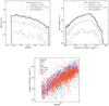 |
Fig. 1. Distribution of redshift, z, and intrinsic 2 − 10 keV X-ray luminosity, LX, of the combined X-ray AGN sample with spectroscopic redshifts 0.3 ≤ z < 3 and LX > 1042 erg s−1. The top-left panel shows the redshift distribution for the obscuration samples selected via hydrogen column density, NH, as indicated in the legend. The vertical red line indicates the low and high redshift bins. The top-right panel shows the distribution of LX using the same line styles. The bottom panel shows the redshift against the intrinsic 2 − 10 keV X-ray luminosity; different colors and markers indicate the various surveys used. |
Number of AGNs with secure spectroscopic redshifts (third column) per survey for the eight surveys used in this study.
For the analysis, we defined three AGN subsamples based on different cuts in NH, which we refer to as unobscured (NH < 1022 cm−2), moderately obscured (1022 ≤ NH/ cm−2 < 1023.5), and highly obscured (NH ≥ 1023.5) sources. It is worth noting that although unobscured, obscured, and highly obscured AGNs are not matched in terms of X-ray luminosity, at each redshift of interest the median LX is similar among the different subsamples.
In addition, in order to study the AGN clustering evolution, we defined two bins in redshift. We divided the full AGN sample based on 0.3 ≤ z < 1.1 and 1.1 ≤ z < 3.0. Both redshift ranges were designed to have a comparable number of objects: 2642 and 2923 for the low and high redshift ranges, respectively.
We also note that the hydrogen column density estimates and the corresponding classification for a given source may vary when using different methodologies (see, e.g., Brightman et al. 2014, their Figs. 18–19) applied to different surveys (e.g., Castelló-Mor et al. 2013). However, our work does not focus on single sources and individual NH measurements and instead provides a statistical study of large samples of unobscured, moderately obscured, and highly obscured AGNs. As shown in Sect. 4.2, we have verified that our results are robust in the sense that removing individual surveys from the analysis and slightly shifting the NH cut does not make a significant difference.
3. Methodology
Here we describe the methodology and models used to quantify the AGN clustering as a function of the obscuration in different redshift bins. In detail, we measured the AGN clustering by using the projected two-point correlation function, wp(rp) (Davis & Peebles 1983), which is independent of redshift space distortions. The estimator requires the construction of a random catalog that acts as an unclustered distribution of sources.
3.1. Random catalog
We constructed random catalogs separately for each field included in the analysis, assigning random redshifts extracted from the smoothed AGN redshift distribution in the considered survey. We used a Gaussian smoothing kernel with σz = 0.3 as a compromise between overfitting features and smoothing out the distribution. We then drew random coordinates in right ascension and declination, discarding or keeping sources based on the inhomogeneous coverage of the considered X-ray survey. The nonuniform coverage is taken into account either by a sensitivity map (detection limit flux) or by exposure time. Using the sensitivity map method set forth by Georgakakis et al. (2008; e.g., Allevato et al. 2011; Viitanen et al. 2019), a random flux was drawn from the flux distribution of the AGN sample for each position, and the random source was kept or discarded based on whether it exceeds the flux limit at that position. We note that due to the survey flux limits, sampling the AGN distribution underpredicts the number of sources with faint fluxes compared to, for example, drawing fluxes directly from the AGN log N − log S. We verified that the correlation function measurement is robust against undersampling the lower fluxes by performing a test where fluxes are instead sampled from the log N − log S as derived by Luo et al. (2017) for 7 Ms CDF-S AGNs. We find the correlation function measurement remains unchanged within the errors.
The sensitivity map method was applied to AEGIS-XD, 4 Ms CDF-S, CDF-N, CDWFS, COSMOS, and XMM-XXL. For 7 Ms CDF-S and X-UDS, we decided to discard random objects based on the effective exposure time at the sky position in a linear manner. In detail, we normalized the exposure at the proposed position to unity based on the maximum value of the exposure map and drew a uniform random number between 0 and 1, which gives the probability of discarding the random source at the position. We note that both these methods are preferable to assigning random positions simply drawn from the distributions of coordinates in the real data catalog directly, which discards the clustering signal in the perpendicular direction (e.g., Gilli et al. 2005; Koutoulidis et al. 2018). For each survey, we constructed a random sample 300 times the size of the data sample.
3.2. Two-point correlation function estimator
We measured the two-point correlation function, which measures the excess probability of finding an AGN pair above random at a given physical separation of rp (perpendicular) and π (parallel):
![$$ \begin{aligned} \mathrm{d} P_{12} = n^2 \left[ 1 + \xi (r_{\mathrm{p} }, \pi ) \right] \mathrm{d} V_1 \mathrm{d} V_2, \end{aligned} $$](/articles/aa/full_html/2023/06/aa45320-22/aa45320-22-eq3.gif)
where n is the mean AGN number density, and we estimate ξ(rp, π) using the standard Landy & Szalay (1993) estimator in bins of rp, π as
where dd, dr, and rr correspond to the normalized number of data–data, data–random, and random–random pairs. Then, we estimated the projected two-point correlation function, wp, by integrating along the line of sight up to πmax to get rid of redshift space distortions (Davis & Peebles 1983):
In detail, we estimated wp(rp) using eight logarithmic bins for rp = 0.1 − 100 h−1 Mpc, and with π = 0 − 100 Mpc h−1 (Δπ = 1 h−1 Mpc) for the pairs. In order to prevent integration over (potentially) empty bins, we first integrated the pairs up to πmax along the line of sight before estimating wp(rp). We find πmax ∼ 20 h−1 Mpc to be a good compromise between maximizing the clustering signal and introducing noise into the estimator.
3.3. Large-scale bias and typical dark matter halo mass
The AGN distribution is a biased tracer of the underlying DM distribution. That is, the AGN projected two-point correlation function, wp(rp), is related to the DM one, wp, DM(rp, z), at large scales, rp ≳ 1 Mpc h−1, via the large-scale bias, b:
where wp, DM is estimated using our adopted cosmology and the ΛCDM power spectrum fitting formulae of Eisenstein & Hu (1998). The standard approach used in previous clustering studies (e.g., Hickox et al. 2009) is to derive the large-scale bias factor from Eq. (4) and associate a typical DM halo mass, b(Mhalo, z), according to the ellipsoidal collapse model of Sheth et al. (2001) and the numerical results of van den Bosch (2002). However, in this approach the large-scale structure growth and the evolution of the bias factor with redshift are not properly considered. In order to include the effect of the redshift dependence of the bias associated with our use of large redshift intervals as the structures grow over time, we estimated the bias factor,  , the redshift,
  , and the halo mass, MA11, by using the methodology described by Eqs. (20)–(24) of Allevato et al. (2011). These estimates are weighted by the growth function and include only the AGN pairs that contribute to the AGN large-scale clustering. Table 2 shows the weighted bias,
  , weighted redshift,
  , and the corresponding DM halo mass, MA11, for all the different subsamples considered in this analysis. It is worth noting that
  is defined with respect to the DM correlation function at z = 0 (wp, DM(rp, z = 0)) and thus cannot be directly compared to the large-scale bias derived in Eq. (4). For this reason, following Allevato et al. (2011), we also estimated the bA11 bias associated with MA11 according to Sheth et al. (2001). This bias factor can be seen as properly corrected for the large-scale structure growth and the evolution of the bias factor within the wide redshift bins considered. As shown in Table 2, bA11 is ∼10–20% smaller than b2 − halo (see Table 2).
Number of X-ray AGNs divided into bins of redshift and obscuration, and the results of the large-scale bias model.
We note that the typical DM halo mass derived from the large-scale bias may not reflect the true distribution of AGN host halo masses. This is especially the case if the underlying AGN host halo mass distribution spans a range of halo masses in different large-scale environments. For example, Leauthaud & Benson (2015) find a skewed distribution of AGN host halo DM masses in COSMOS, where the typical DM halo masses reported earlier varied between their median (lower) and mean (higher) values. Also, using DM halos from large N-body simulations and empirically motivated AGN models, Aird & Coil (2021) find that the true bias calculated directly from the DM halos is systematically lower than the observationally measured one. However, in their semi-analytic AGN model, Oogi et al. (2020) find that there is little difference in the large-scale bias derived from the projected two-point correlation function and the halo occupation distribution, which in turn is sensitive to the halo mass distribution. While conclusions about the typical AGN environment based on large-scale bias alone may be limited, the main focus of this work is to point out relative differences in AGN populations in terms of redshift and obscuration, which is more robust against the aforementioned limitations.
3.4. Uncertainty estimation
In order to estimate the two-point correlation function errors, as well as the subsequent errors on the large-scale bias and the typical DM halo mass, we used a bootstrap resampling method. In detail, we divided the combined AGN sample into non-overlapping regions based on right ascension and the sine of declination. The number of regions defined for each survey was selected so that the sky area and number of objects per region are comparable, and the total number of regions ranges from 1 (pencil beams, e.g., 7 Ms CDF-S) to 36 (XMM-XXL). Then, we randomly resampled the regions with replacement in order to construct Nb = 300 mock samples (e.g., Norberg et al. 2009). For each bootstrap sample, k, constructed in this way, we estimated  using Eqs. (2) and (3) and constructed the bootstrap covariance matrix via
where i, j refer to bins of rp. The large-scale bias was then estimated for each bootstrap sample using χ2 minimization, namely minimizing ΔTC−1Δ, where Δ is the difference between the data and the model (Eq. (4)) and C−1 is the inverse of the covariance matrix. For the projected two-point correlation function, the large-scale bias, and the typical DM halo mass, we report the errors as the 16%,50%, and 84% percentiles of the bootstrap distribution based on Nb = 300 samples.
4. Results
4.1. Clustering as a function of obscuration and redshift
We divided the AGN sample into two redshift bins: 0.3 ≤ z < 1.1 and 1.1 ≤ z < 3.0, which we refer to as the low and high redshift samples in the following (see Table 2). The two bins are defined to contain a comparable number of AGNs with N = 2642 and 2923 for the low and high redshift intervals. We note that changing the exact cut in redshift by ±0.2 corresponds to a difference of ∼5 − 10% in the large-scale bias.
For each redshift bin we defined three AGN subsamples based on different cuts in NH, which we refer to as unobscured (NH < 1022 cm−2), moderately obscured (1022 ≤ NH/cm−2 < 1023.5), and highly obscured (NH ≥ 1023.5) sources. We also note that in the 2 Ms CDF-N and 7 Ms CDF-S, Li et al. (2020) only report the X-ray spectral analysis for moderately to highly obscured AGNs with NH > 1023 cm−2. A difference of ±0.2 dex in the NH cut corresponds to a difference of ∼5 − 10% in the large-scale bias estimates and does not change the overall trend of our results. It is worth noting that the NH cut at 1023.5 cm−2 (compared to the NH > 1024 cm−2 cut that defines the CTK AGN regime) is driven by the need to increase the statistics in each AGN subsample. In fact, the highly obscured AGN bin is the most sensitive to the exact choice of the limits in redshift and obscuration, as the number counts decrease rapidly toward higher redshifts and higher obscuration.
We show the estimated AGN projected two-point correlation function, wp(rp), as a function of NH for the entire redshift range and for the low and high redshift intervals in Fig. 2. We then derived the large-scale bias, b(z, NH) (Fig. 3), and the corresponding typical DM halo mass (Fig. 4) at different obscuration cuts and redshifts using the two different methodologies described in Sect. 3. We focus our discussion on the results based on the methodology put forth by Allevato et al. (2011), and provide the two-halo large-scale bias and the corresponding typical DM halo mass for reference. We summarize all the estimates in Table 2. It is worth noting that by modeling the large-scale clustering, only a typical mass of the hosting halos can be derived; it may not be representative of the entire hosting halo mass distribution of the considered AGN sample. Only the modeling of the small-scale signal can provide this information.
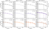 |
Fig. 2. Measured two-point correlation function in redshift (rows) and obscuration bins (columns). Each figure shows the wp(rp), with error bars corresponding to the 1σ derived from bootstrap resampling. The best-fit weighted bias, |

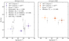 |
Fig. 3. Large-scale bias as a function of redshift (panels) and obscuration (markers in accordance with the legend). The vertical error bars correspond to the 16% and 84% quantiles of the best-fit bias using bootstrap resampling. The horizontal error bars show the 1σ of the NH distribution of the sample. Measurements from X-ray AGN clustering in terms of the HR at comparable redshifts are shown as gray markers in accordance with the legend (Gilli et al. 2009; Allevato et al. 2011; Mendez et al. 2016; Koutoulidis et al. 2018). Note that for plotting purposes we assume NH = 1021 cm−2 (NH = 1023 cm−2) for the soft (hard) samples and include a slight offset in NH for visual clarity. With open markers we show the bias based on the correlation length measurement, r0, assuming a power-law index γ = 1.8, as reported by Gilli et al. (2009), Allevato et al. (2011), Mendez et al. (2016), and Koutoulidis et al. (2018). |
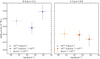 |
Fig. 4. Typical DM halo mass as a function of redshift. The colors and markers carry the same meaning as in Fig. 3. |
At high redshift we find no dependence of the AGN large-scale bias on the level of obscuration of NH. In terms of the corresponding DM hosting halos, our results show, for the first time, that unobscured and moderately to highly obscured AGNs reside in the same environment at z ∼ 1.8, at any NH. At low redshift, z ∼ 0.7, moderately obscured AGNs are slightly less biased ( ) than highly obscured sources (
 ), but the bias estimates are consistent within the error bars.
Figure 5 shows the large-scale bias and the corresponding typical mass of the hosting halos as a function of redshift for all the AGN samples with different NH cuts. We find that the typical mass of the hosting halos decreases with redshift irrespective of the obscuration cut. In detail, the halo mass of unobscured (highly obscured) AGNs decreases with increasing redshift, going from ![$ \log {M_{\mathrm{halo}}}\,[h^{-1}\,{M}_\odot] = {12.74}_{-0.11}^{+0.09} ({=}{12.98}_{-0.22}^{+0.17} $](/articles/aa/full_html/2023/06/aa45320-22/aa45320-22-eq106.gif) ) at z ∼ 0.7 to
) at z ∼ 0.7 to  ) at z ∼ 1.8. A similar trend is observed for moderately obscured AGNs.
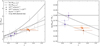 |
Fig. 5. Large-scale bias (left) and typical DM halo mass (right) as a function of redshift and AGN obscuration. The markers and colors correspond to the obscuration bins, in accordance with the legend. The horizontal error bars correspond to 1σ of the redshift distribution. The solid lines show the redshift evolution of the bias for a constant DM halo mass, b(z, Mhalo = const) and for DM halo masses log Mhalo = 12.5 and 13.0 (in units of h−1 M⊙) using the prescriptions of Sheth et al. (2001) and van den Bosch (2002) (labeled Mhalo, const). The dotted lines track the DM halo mass evolution through the accretion rates given by Fakhouri et al. (2010) given a present-day DM halo mass of log Mhalo = 12.8, 13.2 (in h−1 M⊙, labeled Mhalo, acc). The gray markers show the X-ray-selected AGN bias measurements as reported by Aird & Coil (2021, see the text for the details). |
4.2. Different combination of the input surveys
We further explored whether our results are affected by combining in the analysis different surveys and/or NH derivation methodologies. For this, we performed recalculations of the projected two-point correlation function and the corresponding large-scale bias, leaving out one or more surveys at a time. In detail, we considered the following cases, removing from the analysis: (i) 2 Ms CDF-N and 7 Ms CDF-S AGNs from the catalog of Li et al. (2020), which only includes sources with log NH > 23.0; (ii) XMM-XXL AGNs (i.e., we omit the only XMM-Newton survey included in this work); (iii) CDWFS AGNs for which the obscuration NH has been estimated by using the HR instead of X-ray spectral analysis; and (iv) CCL AGNs, given the overdensities caused by large structures present in the COSMOS field (e.g., Gilli et al. 2009; Mendez et al. 2016). As final test, we included in the analysis only the AGN catalog presented in Brightman et al. (2014), which includes the AEGIS-XD, 4 Ms CDF-S, C-COSMOS, and X-UDS (Kocevski et al. 2018) fields and where the X-ray spectral analyses are all performed using the same methodology. We summarize the results of these tests in Fig. 6.
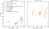 |
Fig. 6. Large-scale bias as a function of hydrogen column density, NH, when excluding different surveys from the combined AGN sample. In each set, the leftmost point shows the original reported result when including all eight surveys in the analysis. The adjacent open symbols (offset slightly for visual clarity) correspond to when one or more surveys are left out of the combined sample. The circles correspond to when CDF-S 7 Ms and CDF-N AGNs are excluded (Li et al. 2020). Squares, diamonds, and triangles correspond to when AGNs from XMM-XXL, CDWFS, and CCL are excluded, respectively. Finally, star symbols correspond to when we include only the surveys considered in Brightman et al. (2014), i.e., AEGIS-XD, 4 Ms CDF-S, C-COSMOS, and X-UDS (Kocevski et al. 2018). See Sect. 4.2 for details. |
In summary, we find that our results in terms of large-scale bias as a function of obscuration NH do not depend on whether or not we include AGNs with NH derived from the HR. Similar results are obtained when excluding from the analysis XMM-XXL and CCL AGNs. Since the statistics rapidly decrease when moving to higher redshifts and higher NH cuts, the sample of highly obscured AGNs at high redshifts, z ∼ 1.8, is the most affected by the particular combination of surveys used. In fact, as expected, the data points at z ∼ 1.8 for highly obscured AGNs show a larger scatter. Furthermore, a larger bias is found when only the AGN catalogs described in Brightman et al. (2014) and Kocevski et al. (2018) are included in the analysis.
5. Discussion
In this work we measure the clustering properties as a function of obscuration, defined in terms of hydrogen column density (NH) or HR, of one of the largest compilations of X-ray-selected AGNs from eight deep XMM/Chandra and multiwavelength surveys. For the first time, in addition to measuring the clustering of unobscured (NH < 1022 cm−2) and moderately obscured AGNs (1022 ≤ NH/cm−2 < 1023.5), we also targeted highly obscured AGNs (≥1023.5 cm−2). Here we discuss our results in a larger context.
5.1. Unobscured versus moderately obscured AGNs
We find that the AGN large-scale bias is independent of the obscuration level of NH at z ∼ 1.8. A small deviation from this trend is observed for highly obscured AGNs, which are slightly more biased than their less obscured counterparts at z ∼ 0.7 (see Fig. 3). However, the bias estimates are consistent within the error bars.
Previous studies at different redshifts show controversial results, namely unobscured sources being more biased than moderately obscured ones (Cappelluti et al. 2010; Allevato et al. 2011, 2014), or no significant difference in the large-scale clustering of the two populations (Gilli et al. 2009; Ebrero et al. 2009; Coil et al. 2009; Krumpe et al. 2012; Mendez et al. 2016; Mountrichas & Georgakakis 2012). However, the fact that in these works AGNs are classified as obscured or unobscured sources based on different methods (e.g., the HR, WISE colors, and optical spectroscopy) might bias the results since, for example, the optical type classification does not perfectly match the X-ray classification (Merloni et al. 2014).
Our AGN sample and chosen methodology are similar to those in the recent work by Koutoulidis et al. (2018). They measured the clustering of 736 (720) unobscured (obscured) X-ray-selected AGNs in five deep Chandra fields over 0.6 < z < 1.4 and with mean LX ∼ 1043 erg s−1. At this redshift, z ∼ 1, they find obscured sources (NH > 1022 cm−2) classified via the HR to be slightly more clustered than unobscured AGNs. However, their trend might be driven by highly obscured AGNs, which we find to be slightly more clustered compared to moderately obscured AGNs.
Similarly, the majority of infrared-selected AGN clustering studies find that obscured sources are located in more massive halos than their unobscured counterparts (Hickox et al. 2011; Donoso et al. 2014; DiPompeo et al. 2014, 2015, 2016, 2017). However, it is worth noting that these studies use different wavelengths to select and classify AGNs. In fact, Koutoulidis et al. (2018) show that the optical/infrared criterion fails to identify a pure AGN sample and that obscured quasars based on optical/infrared colors may equally contain X-ray-unobscured and X-ray-obscured AGNs. Mountrichas et al. (2021) infer that optical/mid-infrared color criteria are better suited for infrared-selected AGNs and that their efficiency drops for the low to moderate luminosity sources included in X-ray samples.
In this work, instead, the AGN classification is based on the column density, NH, which is more robust in identifying obscured sources in samples of moderate luminosity AGNs, compared to those based on HR and/or infrared/optical criteria. Moreover, this analysis includes, for the first time, highly obscured AGNs with NH ≥ 1023.5 cm−2. Our results are in disagreement with a picture in which obscured AGNs are located in denser environments than unobscured sources (Koutoulidis et al. 2018; Hickox et al. 2011; Donoso et al. 2014; DiPompeo et al. 2016, 2017), which has been interpreted in previous studies (King 2010; Hickox et al. 2011) as BH mass growth lagging behind that of the hosting halo.
On the contrary, our results suggest no significant dependence of the AGN clustering properties on the obscuration, in agreement with AGN unified models, in which whether the AGN is observed as obscured or unobscured depends only on viewing angle, and in which, statistically, the halo-scale environments should be the same for both populations. While we do find a slightly higher large-scale bias for the highly obscured AGNs compared to moderately obscured AGNs at low z, it is still consistent within the errors.
It is worth noting that orientation-based models are oversimplified. In fact, the orientation with respect to a nuclear obscuring torus might not be the main driver of the differences between obscured and unobscured AGNs at any redshift. We know that the circumnuclear geometry is not the only factor, as there is a dependence of the obscuration on the luminosity, Eddington ratio, and galaxy and BH masses (e.g., Ricci et al. 2017a; Lanzuisi et al. 2017). Moreover, the AGN obscuration might also occur on host galaxy scales and be related to the overall galaxy evolution. Intrinsic differences in terms of, for example, the host galaxy stellar mass and BH mass between unobscured and moderately to highly obscured AGNs may also exist. Despite all this, it is noteworthy that our results suggest a negligible dependence of the AGN large-scale bias on the obscuration NH.
On the other hand, according to the evolutionary models, different levels of obscuration correspond to different stages of the growth of BHs and galaxy evolution (Ciotti & Ostriker 1997; Di Matteo et al. 2005; Gilli et al. 2007; Hopkins et al. 2006; Lapi et al. 2006; Bournaud et al. 2007; Somerville et al. 2008; Treister et al. 2009; Fanidakis et al. 2011). In AGN evolutionary models, obscured AGNs are an evolutionary phase of merger-driven BH fueling, in which the AGN is first obscured, followed by an unobscured phase after a gas blowout. However, while these models can explain unobscured AGNs in more massive halos than moderately obscured sources (or vice versa; see, e.g., DiPompeo et al. 2017), this key prediction might be at odds with the lack of significant dependence on obscuration we find here.
Investigation of the clustering properties of larger samples of moderately and, in particular, highly obscured AGNs matched in terms of stellar and BH mass distributions across a wide range of redshift and luminosity would be fundamental to better understanding obscured AGNs. Current and future surveys, such as eROSITA (Merloni et al. 2012), will definitely increase the number of moderately to highly obscured AGNs available for clustering studies.
5.2. Small-scale clustering of obscured AGNs
Alternatively, there are studies of Swift-BAT (Baumgartner et al. 2013) X-ray AGNs in the local Universe, suggesting that unobscured and obscured AGNs (defined according to NH) mainly differ in terms of small-scale clustering (one-halo term) at rp ≲ 0.5 − 1.0 h−1 Mpc, which is due to the clustering of AGN pairs within the same DM halos (Krumpe et al. 2018; Powell et al. 2018). The modeling of this signal puts constraints on the halo occupation distribution, that is to say, on how AGNs populate central and satellite halos.
We find that at small scales, moderately obscured sources might have a slightly higher clustering signal than unobscured sources, at least at low redshifts of z ∼ 0.7 (see Fig. 2). This result, in terms of the one-halo term, might also reflect (or be due to) the observed difference in the bias of moderately obscured compared to unobscured AGNs. Unfortunately, for highly obscured sources, the one-halo term is measured with a large uncertainty.
Following Powell et al. (2018), one possible explanation is that the number of AGNs in satellite galaxies grows with a steeper slope for obscured AGNs than for unobscured AGNs. This means that at a fixed halo mass, the probability of obscured AGNs being in satellite galaxies is higher than that of unobscured sources. In particular, Powell et al. (2018) and Krumpe et al. (2018) argue that the dominant triggering mechanism of obscured AGNs in groups and clusters is not mergers (as the merging cross section decreases in the high relative velocity encounters) but more likely disturbances due to close encounters and/or secular processes.
Differences in halo concentration can also explain the different small-scale clustering signal of the two populations, with obscured AGNs more concentrated than their unobscured counterparts (Gatti et al. 2016; Powell et al. 2018). Highly concentrated halos of a given mass would have a high concentration of satellite galaxies and therefore have a higher probability of galaxy interactions, such as minor mergers and encounters. For instance, Jiang et al. (2016) report significantly more satellites around narrow-line Type 1 AGNs compared to broad-line Type 1 AGNs in the SDSS at low redshifts, z < 0.09.
Future and current surveys will significantly increase the number of moderately to heavily obscured AGNs, allowing us to measure the AGN clustering signal with higher accuracy at small scales, and to extend the modeling of the one-halo term to higher redshifts than previous studies of AGNs in the local Universe.
5.3. Redshift evolution
In Fig. 5 we show the redshift evolution of the AGN bias and the corresponding typical DM halo mass for the different AGN samples, as summarized in Table 2. In addition, we plot a compilation of previous X-ray AGN clustering results from LX-limited samples with varying numbers of AGNs at 0.3 ≲ z ≲ 2 as presented by Aird & Coil (2021). The references are given in Aird & Coil (2021, Fig. 11). For comparison, we also show the halo mass evolution tracks when using (i) the bias evolution assuming a constant halo mass (dashed line) as a function of redshift (Sheth et al. 2001; van den Bosch 2002) and (ii) the halo mass accretion history (dotted line) assuming the accretion rate of Fakhouri et al. (2010), based on the Millennium-II N-body simulation.
We measured, for the first time, the large-scale bias and the typical mass of the hosting halos for highly obscured AGNs and find that these objects reside in dense environments typical of galaxy groups at low (z ∼ 0.7) and high (z ∼ 1.8) redshifts. In particular, we find that the redshift evolution of the AGN bias of unobscured and moderately obscured AGNs follows a passive evolution track, implying that for these AGNs the clustering is mainly driven by the growth rate of the host halos and galaxies across cosmic time. Following the mass accretion rate of Fakhouri et al. (2010), this corresponds to DM halos with Mhalo(z = 1.8)∼1012.3 M⊙ h−1 that evolves into Mhalo(z = 0.7)∼1012.6 M⊙ h−1. A small deviation is observed for highly obscured AGNs, but given the large error bars, a passive evolution with redshift is still consistent with the data.
Determining whether the BH growth in highly obscured AGNs is driven by the host galaxy evolution while in moderately obscured AGNs it is regulated by a constant DM halo mass required to host the AGN activity requires further investigation. In fact, studies connecting galaxy stellar and halo masses indicate that a similar halo mass growth as a function of redshift corresponds to a fixed stellar mass of ∼1011 M⊙ (i.e., above the knee of the stellar-to-halo mass relation; Leauthaud et al. 2012; Shuntov et al. 2022). The similar behavior for X-ray AGNs found here could suggest that AGN activity is more closely linked to the host galaxy stellar mass rather than the DM halo. As already discussed in previous sections, a study of moderately to highly obscured AGNs with known host galaxy and BH properties is required.
6. Conclusions
In this work we have measured the clustering properties of unobscured, obscured, and (for the first time) highly obscured AGNs by compiling one of the largest available samples of X-ray-selected AGNs from deep XMM-Newton/Chandra surveys with known hydrogen column densities, NH, derived from X-ray spectral analysis and/or the X-ray HR. We divided the sample into two redshift bin, z ∼ 0.7 and z ∼ 1.8, and analyzed the clustering for unobscured (NH < 1022 cm−2), moderately obscured (1022 ≤ NH < 1023.5 cm−2), and highly obscured (NH ≥ 1023.5 cm−2) AGNs separately. We summarize our findings as follows.
-
(1)
We find that, irrespective of obscuration, the typical DM halo mass of X-ray AGN samples is Mhalo ∼ 1012.5 − 13 h−1 M⊙, similar to group-scale environments and in line with previous works of X-ray-selected AGNs.
-
(2)
At low (z ∼ 0.7) and high (z ∼ 1.8) redshifts, our results suggest an AGN large-scale bias independent of the obscuration NH. A slightly larger bias is measured for highly obscured AGNs at low z, but it is still consistent within the errors. Despite the fact that orientation-based models are oversimplified and that the obscuration depends on host galaxy and BH properties, it is noteworthy that our results suggest a negligible dependence of the AGN large-scale bias on the obscuration NH.
-
(3)
We estimated, for the first time, the large-scale bias and the typical mass of the hosting halos for highly obscured AGNs and find that these objects reside in DM halos with a typical mass log Mhalo[M⊙/h] ∼ 13.0 (12.3) at a low (high) redshifts, z ∼ 0.7 (1.8).
-
(4)
We find that the redshift evolution of the AGN bias follows a passive evolution track irrespective of obscuration, implying that for these AGNs the clustering is mainly driven by the growth rate of the hosting halos and galaxies with time.
Our work can be easily extended by including the future and ongoing X-ray surveys with spectroscopic follow-ups. The increase in number counts will be especially important for the CTK AGNs. Such surveys include eROSITA, which is already underway and is expected to yield a sample of a few million AGNs up to z ∼ 6, and the future survey by Athena (e.g. Nandra et al. 2013) and/or AXIS (Mushotzky et al. 2019), which are expected to detect ∼20 000 AGNs at z > 3 and at different levels of obscuration.
The Chandra images, background, effective exposure time, and sensitivity maps of AEGIS-XD are available at https://www.mpe.mpg.de/XraySurveys
The corresponding Chandra maps for the 4 Ms (7 Ms) CDF-S are available at https://www.mpe.mpg.de/XraySurveys (http://www2.astro.psu.edu/users/niel/cdfs/cdfs-chandra.html; Luo et al. 2017).
The X-UDS Chandra maps are available at https://www.mpe.mpg.de/XraySurveys.
Acknowledgments
AV acknowledges support from the Vilho, Yrjö and Kalle Väisälä Foundation of the Finnish Academy of Science and Letters. VA acknowledges support from INAF-PRIN 1.05.01.85.08. FS acknowledges partial support from the European Union’s Horizon 2020 research and innovation programme under the Marie Skłodowska-Curie grant agreement No. 860744.
References
- Aird, J., & Coil, A. L. 2021, MNRAS, 502, 5962 [NASA ADS] [CrossRef] [Google Scholar]
- Alexander, D. M., Bauer, F. E., Brandt, W. N., et al. 2003, AJ, 126, 539 [Google Scholar]
- Allevato, V., Finoguenov, A., Cappelluti, N., et al. 2011, ApJ, 736, 99 [NASA ADS] [CrossRef] [Google Scholar]
- Allevato, V., Finoguenov, A., Civano, F., et al. 2014, ApJ, 796, 4 [NASA ADS] [CrossRef] [Google Scholar]
- Antonucci, R. 1993, ARA&A, 31, 473 [Google Scholar]
- Ballantyne, D. R., Shi, Y., Rieke, G. H., et al. 2006, ApJ, 653, 1070 [NASA ADS] [CrossRef] [Google Scholar]
- Baumgartner, W. H., Tueller, J., Markwardt, C. B., et al. 2013, ApJS, 207, 19 [Google Scholar]
- Bournaud, F., Elmegreen, B. G., & Elmegreen, D. M. 2007, ApJ, 670, 237 [Google Scholar]
- Brightman, M., & Nandra, K. 2011, MNRAS, 413, 1206 [NASA ADS] [CrossRef] [Google Scholar]
- Brightman, M., & Ueda, Y. 2012, MNRAS, 423, 702 [NASA ADS] [CrossRef] [Google Scholar]
- Brightman, M., Nandra, K., Salvato, M., et al. 2014, MNRAS, 443, 1999 [NASA ADS] [CrossRef] [Google Scholar]
- Buchner, J., Georgakakis, A., Nandra, K., et al. 2015, ApJ, 802, 89 [Google Scholar]
- Cappelluti, N., Brusa, M., Hasinger, G., et al. 2009, A&A, 497, 635 [NASA ADS] [CrossRef] [EDP Sciences] [Google Scholar]
- Cappelluti, N., Ajello, M., Burlon, D., et al. 2010, ApJ, 716, L209 [NASA ADS] [CrossRef] [Google Scholar]
- Castelló-Mor, N., Carrera, F. J., Alonso-Herrero, A., et al. 2013, A&A, 556, A114 [NASA ADS] [CrossRef] [EDP Sciences] [Google Scholar]
- Ciotti, L., & Ostriker, J. P. 1997, ApJ, 487, L105 [NASA ADS] [CrossRef] [Google Scholar]
- Civano, F., Marchesi, S., Comastri, A., et al. 2016, ApJ, 819, 62 [Google Scholar]
- Coil, A. L., Georgakakis, A., Newman, J. A., et al. 2009, ApJ, 701, 1484 [NASA ADS] [CrossRef] [Google Scholar]
- Davis, M., & Peebles, P. J. E. 1983, ApJ, 267, 465 [Google Scholar]
- Di Matteo, T., Springel, V., & Hernquist, L. 2005, Nature, 433, 604 [NASA ADS] [CrossRef] [Google Scholar]
- DiPompeo, M. A., Myers, A. D., Hickox, R. C., Geach, J. E., & Hainline, K. N. 2014, MNRAS, 442, 3443 [NASA ADS] [CrossRef] [Google Scholar]
- DiPompeo, M. A., Myers, A. D., Hickox, R. C., et al. 2015, MNRAS, 446, 3492 [Google Scholar]
- DiPompeo, M. A., Hickox, R. C., & Myers, A. D. 2016, MNRAS, 456, 924 [NASA ADS] [CrossRef] [Google Scholar]
- DiPompeo, M. A., Hickox, R. C., Eftekharzadeh, S., & Myers, A. D. 2017, MNRAS, 469, 4630 [NASA ADS] [CrossRef] [Google Scholar]
- Donoso, E., Yan, L., Stern, D., & Assef, R. J. 2014, ApJ, 789, 44 [NASA ADS] [CrossRef] [Google Scholar]
- Ebrero, J., Mateos, S., Stewart, G. C., Carrera, F. J., & Watson, M. G. 2009, A&A, 500, 749 [NASA ADS] [CrossRef] [EDP Sciences] [Google Scholar]
- Eisenstein, D. J., & Hu, W. 1998, ApJ, 496, 605 [Google Scholar]
- Elyiv, A., Clerc, N., Plionis, M., et al. 2012, A&A, 537, A131 [NASA ADS] [CrossRef] [EDP Sciences] [Google Scholar]
- Fakhouri, O., Ma, C.-P., & Boylan-Kolchin, M. 2010, MNRAS, 406, 2267 [Google Scholar]
- Fanidakis, N., Baugh, C. M., Benson, A. J., et al. 2011, MNRAS, 410, 53 [NASA ADS] [CrossRef] [Google Scholar]
- Gatti, M., Shankar, F., Bouillot, V., et al. 2016, MNRAS, 456, 1073 [NASA ADS] [CrossRef] [Google Scholar]
- Geach, J. E., Hickox, R. C., Bleem, L. E., et al. 2013, ApJ, 776, L41 [Google Scholar]
- Georgakakis, A., Nandra, K., Laird, E. S., Aird, J., & Trichas, M. 2008, MNRAS, 388, 1205 [Google Scholar]
- Georgantopoulos, I., Comastri, A., Vignali, C., et al. 2013, A&A, 555, A43 [NASA ADS] [CrossRef] [EDP Sciences] [Google Scholar]
- Gilli, R., Daddi, E., Zamorani, G., et al. 2005, A&A, 430, 811 [NASA ADS] [CrossRef] [EDP Sciences] [Google Scholar]
- Gilli, R., Comastri, A., & Hasinger, G. 2007, A&A, 463, 79 [NASA ADS] [CrossRef] [EDP Sciences] [Google Scholar]
- Gilli, R., Zamorani, G., Miyaji, T., et al. 2009, A&A, 494, 33 [NASA ADS] [CrossRef] [EDP Sciences] [Google Scholar]
- Gilli, R., Norman, C., Calura, F., et al. 2022, A&A, 666, A17 [NASA ADS] [CrossRef] [EDP Sciences] [Google Scholar]
- Grogin, N. A., Kocevski, D. D., Faber, S. M., et al. 2011, ApJS, 197, 35 [NASA ADS] [CrossRef] [Google Scholar]
- Hasinger, G. 2008, A&A, 490, 905 [NASA ADS] [CrossRef] [EDP Sciences] [Google Scholar]
- Hasinger, G., Cappelluti, N., Brunner, H., et al. 2007, ApJS, 172, 29 [NASA ADS] [CrossRef] [Google Scholar]
- Hickox, R. C., Jones, C., Forman, W. R., et al. 2009, ApJ, 696, 891 [Google Scholar]
- Hickox, R. C., Myers, A. D., Brodwin, M., et al. 2011, ApJ, 731, 117 [NASA ADS] [CrossRef] [Google Scholar]
- Hönig, S. F., Kishimoto, M., Tristram, K. R. W., et al. 2013, ApJ, 771, 87 [Google Scholar]
- Hopkins, P. F., Hernquist, L., Cox, T. J., et al. 2006, ApJS, 163, 1 [Google Scholar]
- Hopkins, P. F., Hernquist, L., Cox, T. J., & Kereš, D. 2008, ApJS, 175, 356 [Google Scholar]
- Jiang, N., Wang, H., Mo, H., et al. 2016, ApJ, 832, 111 [Google Scholar]
- King, A. R. 2010, MNRAS, 408, L95 [Google Scholar]
- Kocevski, D. D., Hasinger, G., Brightman, M., et al. 2018, ApJS, 236, 48 [CrossRef] [Google Scholar]
- Koutoulidis, L., Georgantopoulos, I., Mountrichas, G., et al. 2018, MNRAS, 481, 3063 [NASA ADS] [CrossRef] [Google Scholar]
- Krumpe, M., Miyaji, T., Coil, A. L., & Aceves, H. 2012, ApJ, 746, 1 [NASA ADS] [CrossRef] [Google Scholar]
- Krumpe, M., Miyaji, T., Coil, A. L., & Aceves, H. 2018, MNRAS, 474, 1773 [CrossRef] [Google Scholar]
- La Franca, F., Fiore, F., Comastri, A., et al. 2005, ApJ, 635, 864 [NASA ADS] [CrossRef] [Google Scholar]
- Laird, E. S., Nandra, K., Georgakakis, A., et al. 2009, ApJS, 180, 102 [NASA ADS] [CrossRef] [Google Scholar]
- Landy, S. D., & Szalay, A. S. 1993, ApJ, 412, 64 [Google Scholar]
- Lanzuisi, G., Delvecchio, I., Berta, S., et al. 2017, A&A, 602, A123 [NASA ADS] [CrossRef] [EDP Sciences] [Google Scholar]
- Lanzuisi, G., Civano, F., Marchesi, S., et al. 2018, MNRAS, 480, 2578 [Google Scholar]
- Lapi, A., Shankar, F., Mao, J., et al. 2006, ApJ, 650, 42 [Google Scholar]
- Leauthaud, A., Tinker, J., Bundy, K., et al. 2012, ApJ, 744, 159 [Google Scholar]
- Leauthaud, A., Benson, J. A., Civano, F., et al. 2015, MNRAS, 446, 1874 [NASA ADS] [CrossRef] [Google Scholar]
- Li, J., Xue, Y., Sun, M., et al. 2019, ApJ, 877, 5 [NASA ADS] [CrossRef] [Google Scholar]
- Li, J., Xue, Y., Sun, M., et al. 2020, ApJ, 903, 49 [NASA ADS] [CrossRef] [Google Scholar]
- Liu, Z., Merloni, A., Georgakakis, A., et al. 2016, MNRAS, 459, 1602 [Google Scholar]
- Luo, B., Brandt, W. N., Xue, Y. Q., et al. 2017, ApJS, 228, 2 [Google Scholar]
- Marchesi, S., Civano, F., Elvis, M., et al. 2016, ApJ, 817, 34 [Google Scholar]
- Masini, A., Hickox, R. C., Carroll, C. M., et al. 2020, ApJS, 251, 2 [Google Scholar]
- Mendez, A. J., Coil, A. L., Aird, J., et al. 2016, ApJ, 821, 55 [NASA ADS] [CrossRef] [Google Scholar]
- Menzel, M. L., Merloni, A., Georgakakis, A., et al. 2016, MNRAS, 457, 110 [NASA ADS] [CrossRef] [Google Scholar]
- Merloni, A., Predehl, P., Becker, W., et al. 2012, ArXiv e-prints [arXiv:1209.3114] [Google Scholar]
- Merloni, A., Bongiorno, A., Brusa, M., et al. 2014, MNRAS, 437, 3550 [Google Scholar]
- Mountrichas, G., & Georgakakis, A. 2012, MNRAS, 420, 514 [NASA ADS] [CrossRef] [Google Scholar]
- Mountrichas, G., Buat, V., Georgantopoulos, I., et al. 2021, A&A, 653, A70 [NASA ADS] [CrossRef] [EDP Sciences] [Google Scholar]
- Murphy, K. D., & Yaqoob, T. 2009, MNRAS, 397, 1549 [Google Scholar]
- Mushotzky, R., Aird, J., Barger, A. J., et al. 2019, Bull. Am. Astron. Soc., 51, 107 [Google Scholar]
- Nandra, K., Georgakakis, A., Willmer, C. N. A., et al. 2007, ApJ, 660, L11 [NASA ADS] [CrossRef] [Google Scholar]
- Nandra, K., Barret, D., Barcons, X., et al. 2013, ArXiv e-prints [arXiv:1306.2307] [Google Scholar]
- Nandra, K., Laird, E. S., Aird, J. A., et al. 2015, ApJS, 220, 10 [NASA ADS] [CrossRef] [Google Scholar]
- Netzer, H. 2015, ARA&A, 53, 365 [Google Scholar]
- Norberg, P., Baugh, C. M., Gaztañaga, E., & Croton, D. J. 2009, MNRAS, 396, 19 [Google Scholar]
- Oogi, T., Shirakata, H., Nagashima, M., et al. 2020, MNRAS, 497, 1 [NASA ADS] [CrossRef] [Google Scholar]
- Pierre, M., Pacaud, F., Adami, C., et al. 2016, A&A, 592, A1 [NASA ADS] [CrossRef] [EDP Sciences] [Google Scholar]
- Powell, M. C., Cappelluti, N., Urry, C. M., et al. 2018, ApJ, 858, 110 [Google Scholar]
- Rangel, C., Nandra, K., Laird, E. S., & Orange, P. 2013, MNRAS, 428, 3089 [Google Scholar]
- Ricci, C., Trakhtenbrot, B., Koss, M. J., et al. 2017a, Nature, 549, 488 [NASA ADS] [CrossRef] [Google Scholar]
- Ricci, F., Marchesi, S., Shankar, F., La Franca, F., & Civano, F. 2017b, MNRAS, 465, 1915 [CrossRef] [Google Scholar]
- Scoville, N., Aussel, H., Brusa, M., et al. 2007, ApJS, 172, 1 [Google Scholar]
- Sheth, R. K., Mo, H. J., & Tormen, G. 2001, MNRAS, 323, 1 [NASA ADS] [CrossRef] [Google Scholar]
- Shuntov, M., McCracken, H. J., Gavazzi, R., et al. 2022, A&A, 664, A61 [NASA ADS] [CrossRef] [EDP Sciences] [Google Scholar]
- Somerville, R. S., Hopkins, P. F., Cox, T. J., Robertson, B. E., & Hernquist, L. 2008, MNRAS, 391, 481 [NASA ADS] [CrossRef] [Google Scholar]
- Tozzi, P., Gilli, R., Mainieri, V., et al. 2006, A&A, 451, 457 [NASA ADS] [CrossRef] [EDP Sciences] [Google Scholar]
- Treister, E., & Urry, C. M. 2006, ApJ, 652, L79 [NASA ADS] [CrossRef] [Google Scholar]
- Treister, E., Urry, C. M., & Virani, S. 2009, ApJ, 696, 110 [NASA ADS] [CrossRef] [Google Scholar]
- Tristram, K. R. W., Burtscher, L., Jaffe, W., et al. 2014, A&A, 563, A82 [CrossRef] [EDP Sciences] [Google Scholar]
- Ueda, Y., Akiyama, M., Hasinger, G., Miyaji, T., & Watson, M. G. 2014, ApJ, 786, 104 [Google Scholar]
- Urry, C. M., & Padovani, P. 1995, PASP, 107, 803 [NASA ADS] [CrossRef] [Google Scholar]
- van den Bosch, F. C. 2002, MNRAS, 331, 98 [CrossRef] [Google Scholar]
- Viitanen, A., Allevato, V., Finoguenov, A., et al. 2019, A&A, 629, A14 [NASA ADS] [CrossRef] [EDP Sciences] [Google Scholar]
- Wright, E. L., Eisenhardt, P. R. M., Mainzer, A. K., et al. 2010, AJ, 140, 1868 [Google Scholar]
- Xue, Y. Q., Luo, B., Brandt, W. N., et al. 2016, ApJS, 224, 15 [Google Scholar]
- Xue, Y. Q., Luo, B., Brandt, W. N., et al. 2011, ApJS, 195, 10 [Google Scholar]
- Yan, L., Donoso, E., Tsai, C.-W., et al. 2013, AJ, 145, 55 [NASA ADS] [CrossRef] [Google Scholar]
All Tables
Number of AGNs with secure spectroscopic redshifts (third column) per survey for the eight surveys used in this study.
Number of X-ray AGNs divided into bins of redshift and obscuration, and the results of the large-scale bias model.
All Figures
|
Fig. 1. Distribution of redshift, z, and intrinsic 2 − 10 keV X-ray luminosity, LX, of the combined X-ray AGN sample with spectroscopic redshifts 0.3 ≤ z < 3 and LX > 1042 erg s−1. The top-left panel shows the redshift distribution for the obscuration samples selected via hydrogen column density, NH, as indicated in the legend. The vertical red line indicates the low and high redshift bins. The top-right panel shows the distribution of LX using the same line styles. The bottom panel shows the redshift against the intrinsic 2 − 10 keV X-ray luminosity; different colors and markers indicate the various surveys used. |
| In the text | |
|
Fig. 2. Measured two-point correlation function in redshift (rows) and obscuration bins (columns). Each figure shows the wp(rp), with error bars corresponding to the 1σ derived from bootstrap resampling. The best-fit weighted bias, |
| In the text | |
|
Fig. 3. Large-scale bias as a function of redshift (panels) and obscuration (markers in accordance with the legend). The vertical error bars correspond to the 16% and 84% quantiles of the best-fit bias using bootstrap resampling. The horizontal error bars show the 1σ of the NH distribution of the sample. Measurements from X-ray AGN clustering in terms of the HR at comparable redshifts are shown as gray markers in accordance with the legend (Gilli et al. 2009; Allevato et al. 2011; Mendez et al. 2016; Koutoulidis et al. 2018). Note that for plotting purposes we assume NH = 1021 cm−2 (NH = 1023 cm−2) for the soft (hard) samples and include a slight offset in NH for visual clarity. With open markers we show the bias based on the correlation length measurement, r0, assuming a power-law index γ = 1.8, as reported by Gilli et al. (2009), Allevato et al. (2011), Mendez et al. (2016), and Koutoulidis et al. (2018). |
| In the text | |
|
Fig. 4. Typical DM halo mass as a function of redshift. The colors and markers carry the same meaning as in Fig. 3. |
| In the text | |
|
Fig. 5. Large-scale bias (left) and typical DM halo mass (right) as a function of redshift and AGN obscuration. The markers and colors correspond to the obscuration bins, in accordance with the legend. The horizontal error bars correspond to 1σ of the redshift distribution. The solid lines show the redshift evolution of the bias for a constant DM halo mass, b(z, Mhalo = const) and for DM halo masses log Mhalo = 12.5 and 13.0 (in units of h−1 M⊙) using the prescriptions of Sheth et al. (2001) and van den Bosch (2002) (labeled Mhalo, const). The dotted lines track the DM halo mass evolution through the accretion rates given by Fakhouri et al. (2010) given a present-day DM halo mass of log Mhalo = 12.8, 13.2 (in h−1 M⊙, labeled Mhalo, acc). The gray markers show the X-ray-selected AGN bias measurements as reported by Aird & Coil (2021, see the text for the details). |
| In the text | |
|
Fig. 6. Large-scale bias as a function of hydrogen column density, NH, when excluding different surveys from the combined AGN sample. In each set, the leftmost point shows the original reported result when including all eight surveys in the analysis. The adjacent open symbols (offset slightly for visual clarity) correspond to when one or more surveys are left out of the combined sample. The circles correspond to when CDF-S 7 Ms and CDF-N AGNs are excluded (Li et al. 2020). Squares, diamonds, and triangles correspond to when AGNs from XMM-XXL, CDWFS, and CCL are excluded, respectively. Finally, star symbols correspond to when we include only the surveys considered in Brightman et al. (2014), i.e., AEGIS-XD, 4 Ms CDF-S, C-COSMOS, and X-UDS (Kocevski et al. 2018). See Sect. 4.2 for details. |
| In the text | |
Current usage metrics show cumulative count of Article Views (full-text article views including HTML views, PDF and ePub downloads, according to the available data) and Abstracts Views on Vision4Press platform.
Data correspond to usage on the plateform after 2015. The current usage metrics is available 48-96 hours after online publication and is updated daily on week days.
Initial download of the metrics may take a while.