| Issue |
A&A
Volume 632, December 2019
|
|
|---|---|---|
| Article Number | A34 | |
| Number of page(s) | 17 | |
| Section | Cosmology (including clusters of galaxies) | |
| DOI | https://doi.org/10.1051/0004-6361/201834879 | |
| Published online | 22 November 2019 | |
KiDS+VIKING-450: A new combined optical and near-infrared dataset for cosmology and astrophysics⋆
1
Astronomisches Institut, Ruhr-Universität Bochum, Universitätsstr. 150, 44801 Bochum, Germany
e-mail: This email address is being protected from spambots. You need JavaScript enabled to view it.
2
Argelander-Institut für Astronomie, Auf dem Hügel 71, 53121 Bonn, Germany
3
Leiden Observatory, Leiden University, Niels Bohrweg 2, 2333 CA Leiden, The Netherlands
4
Institute for Astronomy, University of Edinburgh, Royal Observatory, Blackford Hill, Edinburgh EH9 3HJ, UK
5
Center for Cosmology and AstroParticle Physics, The Ohio State University, 191 West Woodruff Avenue, Columbus, OH 43210, USA
6
Kapteyn Astronomical Institute, University of Groningen, PO Box 800, 9700 AV Groningen, The Netherlands
7
Centre for Extragalactic Astronomy, Department of Physics, Durham University, South Road, Durham DH1 3LE, UK
8
Institute of Astronomy, University of Cambridge, Madingley Road, Cambridge CB3 0HA, UK
9
INAF – Osservatorio Astronomico di Capodimonte, Via Moiariello 16, 80131 Napoli, Italy
10
School of Physics and Astronomy, Sun Yat-sen University, Zhuhai Campus, Guangzhou 519082, PR China
11
INAF – Osservatorio Astronomico di Padova, Via dell’Osservatorio 5, 35122 Padova, Italy
12
Department of Astrophysical Sciences, Peyton Hall, Princeton University, Princeton, NJ 08544, USA
13
School of Physics and Astronomy, Queen Mary University of London, Mile End Road, London E1 4NS, UK
Received:
14
December
2018
Accepted:
28
August
2019
Abstract
We present the curation and verification of a new combined optical and near infrared dataset for cosmology and astrophysics, derived by combining ugri-band imaging from the Kilo-Degree Survey (KiDS) and ZYJHKs-band imaging from the VISTA Kilo degree Infrared Galaxy (VIKING) survey. This dataset is unrivaled in cosmological imaging surveys due to the combination of its area (458 deg2 before masking), depth (r ≤ 25), and wavelength coverage (ugriZYJHKs). This combination of survey depth, area, and (most importantly) wavelength coverage allows significant reductions in systematic uncertainties (i.e. reductions of between 10% and 60% in bias, outlier rate, and scatter) in photometric-to-spectroscopic redshift comparisons, compared to the optical-only case at photo-z above 0.7. The complementarity between our optical and near infrared surveys means that over 80% of our sources, across all photo-z, have significant detections (i.e. not upper limits) in our eight reddest bands. We have derived photometry, photo-z, and stellar masses for all sources in the survey, and verified these data products against existing spectroscopic galaxy samples. We demonstrate the fidelity of our higher-level data products by constructing the survey stellar mass functions in eight volume-complete redshift bins. We find that these photometrically derived mass functions provide excellent agreement with previous mass evolution studies derived using spectroscopic surveys. The primary data products presented in this paper are made publicly available through the KiDS survey website.
Key words: cosmology: observations / gravitational lensing: weak / galaxies: photometry / surveys
The catalogs are also available at the CDS via anonymous ftp to cdsarc.u-strasbg.fr (130.79.128.5) or via http://cdsarc.u-strasbg.fr/viz-bin/cat/J/A+A/632/A34
© ESO 2019
1. Introduction
Over the last decade, observational cosmological estimates have become increasingly restricted by systematic, rather than random, uncertainties (Hildebrandt et al. 2016, 2019; Troxel et al. 2018; Hikage et al. 2019; Planck Collaboration VI 2019). In particular, estimates made using large photometric samples of galaxies, such as those utilising weak gravitational lensing (see, e.g. Bacon et al. 2000; Van Waerbeke et al. 2000; Wittman et al. 2000; Rhodes et al. 2001), have moved closer to a regime where increasing sample sizes alone are unlikely to cause a significant improvement in estimate constraints (Becker et al. 2016; Jee et al. 2016; Hildebrandt et al. 2017, 2019; Troxel et al. 2018). Instead, quantification and reduction of systematic biases are becoming increasingly important, and more frequently the dominating source of uncertainty in cosmological inference (Mandelbaum 2018).
One such systematic limitation for many methods of observational cosmological inference (and indeed one that frequently dominates the systematic uncertainty budget; Hildebrandt et al. 2016; Hikage et al. 2019) is also one of the most fundamental: that of estimation of source positions in 3-dimensional space. Specifically, localisation of galaxies along the line-of-sight (i.e. distance) axis is of particular importance. This localisation is typically achieved through relatively low-precision photometric based methods, referred to as photometric redshift or photo-z (see Hildebrandt et al. 2010, for a summary of photo-z methods).
One method for deriving photo-z estimates involves finding the model galaxy spectrum, from a sample of representative spectrum templates, which best fits the observed galaxy flux in a series of wavelength bands (Ilbert et al. 2006; Benítez 2000; Brammer et al. 2008; Bolzonella et al. 2000). These estimates are typically restricted by the quality of the input photometry, the intrinsic redshift distribution of the source galaxy sample, and the degeneracy between various galaxy spectrum models as a function of galaxy redshift (Ilbert et al. 2009; Laigle et al. 2019). In each of these cases, however, additional information can lead to significant benefits in the photo-z estimation process.
For cosmological inference, a weak lensing survey needs to provide reliable galaxy shapes (see, e.g. Massey et al. 2007) and redshift estimates for a statistically representative sample of galaxies over cosmologically significant redshifts (see, e.g. Hildebrandt et al. 2019; Troxel et al. 2018; Hikage et al. 2019). For this purpose, there are, therefore, three main properties that determine any weak lensing survey’s cosmological sensitivity: survey area, survey depth, and wavelength coverage. These properties all contribute to both the statistical and systematic uncertainty on cosmological inference. The first two statistics, area and depth, typically govern the raw number of sources in a given redshift interval that can be used for inference. The number of sources is a primary contributor to the statistical uncertainty on cosmic shear cosmological inference, and as such is a key consideration in weak lensing survey design (de Jong et al. 2015; Abbott et al. 2016; Aihara et al. 2018). Similarly, and discussed in more depth below, the wavelength information dictates the limiting photo-z accessible for tomographic binning (Hildebrandt et al. 2019), which is a driving factor in the final signal-to-noise of a cosmic shear estimate. As such, wavelength coverage also contributes non-negligibly to the statistical uncertainty of cosmic shear cosmological estimates. On the systematic effects side, area and depth aid in the constraint of many systematics parameters directly, including the intrinsic alignment signal (Joachimi et al. 2015). Deeper data allow more galaxy satellites to be observed and a better constraint on the galaxy-galaxy intrinsic alignment signal to be made. The wavelength baseline is also a primary driving factor in determining the systematic uncertainty on any cosmological inference, mainly because it dictates the signal-to-noise of the shear signal of individual cosmic shear sources.
There are many reasons why wavelength information is of significant importance in cosmological inference. However we focus on two main reasons for demonstration: namely, reduction of photo-z bias and influence over the redshift baseline. We discuss both of these below.
The importance of wavelength information in the reduction of photo-z bias is driven mostly by the degeneracy between galaxy spectrum models. Even with perfect input photometry, there exist degeneracies between galaxy spectrum models at different redshifts over finite wavelength intervals (see Fig. 1 of Buchs et al. 2019, for a nice demonstration). These degeneracies can lead to considerable biases in the source photo-z distribution, when sources are systematically assigned to incorrect parts of redshift-space. Moreover, these effects are increasingly problematic as source photometry becomes noisier and the wavelength baseline becomes shorter. Naturally, the only way to break such degeneracies is by utilising photometry for these sources that extends beyond the wavelength range wherein the degeneracy exists. As such, longer wavelength baselines are fundamental to the breaking of model degeneracies, and therefore to reducing the systematic incorrect assignment of photo-z. Such incorrect assignment can lead to considerable bias in estimated redshift distributions (Hildebrandt et al. 2019) which limits cosmological inference, over any given source redshift baseline.
Furthermore, wavelength information is the primary factor which determines the useful redshift baseline over which cosmological inference can be performed. In particular, photometry that extends redwards of the optical bands is essential for the accurate estimation of photo-z beyond a redshift of z ∼ 1 (for typical ground-based photometric surveys). This intermediate- to high-redshift information is of particular importance to weak lensing cosmological inference, as higher-redshift sources carry considerably more signal-to-noise than their lower-redshift counterparts. This increased signal is critical in the quantification of systematic bias as it allows them to be explored with reduced stacking of sources (e.g. with finer bins containing more homogeneous samples of galaxies), which can alleviate additional biases.
To date, the largest joint optical and near-infrared (NIR) dataset for cosmology was a combined Dark Energy Survey (DES) + VISTA Hemisphere Survey (VHS) analysis of the DES Science Verification region, covering ∼150 deg2 and spanning the griZYJHKs bands (Banerji et al. 2015). In this paper we present the integration of two European Southern Observatory (ESO) public surveys; the VISTA Kilo degree INfrared Galaxy (VIKING; Edge et al. 2013; Venemans et al. 2015) survey, probing the NIR wavelengths (8000−24 000 Å), and the Kilo Degree Survey (KiDS; Kuij-ken et al. 2015; de Jong et al. 2015), probing optical wavelengths (3000 − 9000 Å). These combined data represent a significant step forwards from the previous state-of-the-art, mainly due to the increase in combined survey area and optimal matching between the two surveys depth (see Sect. 2).
This extension of the wavelength baseline brings with it considerable benefits, particularly for cosmic shear analyses. Hildebrandt et al. (2017) presented cosmological inference from cosmic shear using 450 square degrees of KiDS imaging (referred to as KiDS-450), measuring the matter clustering parameter (σ8) and matter density parameter (Ωm), which are typically parameterised jointly as  , to a relative uncertainty of ∼5%; an error whose budget was limited essentially equally by systematic and random uncertainties. As a result, we expect that the final KiDS dataset, spanning 1350 deg2, will in fact be systematics limited in its cosmological estimates (as random uncertainties should downscale by a factor of roughly
  ). Moreover, constraint and reduction of systematic effects will become of increasing importance in the next few years, and indeed into the next decade with the initiation of large survey programmes such as Euclid (see, e.g. Amendola et al. 2018). Using the combined dataset presented here enables us to make considerable progress regarding the challenge of reducing systematics, and that in doing so enables us to perform an updated cosmic shear analysis which better constrains systematic uncertainties and enables the use of higher-redshift sources (Hildebrandt et al. 2019).
Importantly, this dataset is not only useful for cosmological studies. The additional information provided by the NIR allows better constraint of fundamental galaxy parameters such as stellar mass and star formation rates, which enable the construction of useful samples for galaxy evolution and astrophysics studies. For example, recent use of NIR data in preselection of ultra-compact massive galaxy (UCMG) candidates (Tortora et al. 2018) has allowed the spectroscopic confirmation of the largest sample of UCMGs to date.
As such, this work focusses on the description and verification of the joint KiDS+VIKING photometric dataset, and on the derivation of higher-level data products which are of interest both for weak-lensing cosmological analyses and non-cosmological science use-cases. The KiDS optical and VIKING NIR data and their reduction are described in Sect. 2. The multi-band photometry and estimation of photo-z are covered in Sect. 3. Model fitting to the broadband galaxy spectral energy distributions is given in Sect. 4, as is the exploration of stellar mass estimates from these fits. We compare the resulting stellar mass function for our dataset to previous works in Sect. 5. The paper is summarised in Sect. 6. The primary data products described in this paper are made publicly available1.
2. Dataset and reduction
In this section we describe the KiDS optical (Sect. 2.1) and VIKING NIR (Sect. 2.2) imaging that is used in this study. KiDS and VIKING are partner surveys that will both observe two contiguous patches of sky in the Galactic North and South, covering a combined area of over 1350 square degrees (Arnaboldi et al. 2007; de Jong et al. 2015, 2017). Observations for KiDS are ongoing, and so joint analysis of KiDS+VIKING is currently limited to the footprint of the third KiDS Data Release (de Jong et al. 2017).
The footprint of the post-masking KiDS-450 dataset presented in Hildebrandt et al. (2017) is shown in Fig. 1 both on-sky and split into each of the KiDS “patches” (where each patch contains one of the five ∼ contiguous portions of the KiDS-450 footprint). These individual patches divide the KiDS-450 survey area into five sections of (roughly) contiguous data on-sky, centering mainly on fields observed by the Galaxy And Mass Assembly (GAMA, Driver et al. 2011) redshift survey. The geometry of each patch can be seen in the individual panels of Fig. 1, and are named by the GAMA field on which they are focused. The exception is the GS patch, which has no corresponding GAMA field; we nonetheless maintain the naming convention for convenience. We note, though, that future KiDS observations will close the gaps both within and between the patches, and lead to the creation of a contiguous ∼10 deg × 75 deg stripe in both the Galactic North and South. Observations of these contiguous stripes in VIKING have already been completed.
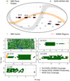 |
Fig. 1. Footprint of the post-masking KiDS-450 dataset. Top: distribution of the KiDS-450 fields on-sky, relative to the Ecliptic and Galactic planes. The Galactic plane is plotted with a width of 20°, which roughly traces the observed width of the Galaxy thick disk. Lower panels: each of the individually named KiDS-450 patches (on their own scale). The points in each patch show the distribution of KiDS-450 photometric sources that remain after applying the bright-star mask. Points are coloured according to their overall observational coverage: green points have full KiDS+VIKING optical and NIR coverage, blue points have full KiDS optical coverage but only partial VIKING NIR coverage, and orange points have KiDS optical coverage only. As such the green and blue data show the footprint of the full KiDS+VIKING-450 (KV450) sample. |
The full (unmasked) KiDS-450 dataset consists of ∼49 million non-unique Galactic and extragalactic sources distributed over 454 overlapping ∼1 deg2 pointings on sky (see Sect. 2.1). This reduces to ∼33.9 million unique mostly-extragalactic sources after applying masking of stars and removing duplicated data, distributed over ∼360 deg2. These unique post-masking sources are shown in Fig. 1, and so the masking around bright stars, for example, can be seen as small circular gaps within the patches. Each source is coloured by its observational coverage statistics: those with full photometric KiDS+VIKING observational coverage are shown in green, those with full KiDS observational coverage but only partial VIKING observational coverage are shown in blue, and those with only KiDS observational coverage are shown in orange. We define the combined KiDS+VIKING-450 sample (hereafter KV450) as those KiDS-450 sources which have overlapping VIKING imaging (i.e. the green sources in Fig. 1). Masking the regions with missing NIR coverage (i.e. the orange and blue data in Fig. 1), the full KV450 footprint consists of 447 overlapping pointings2, covering ∼341 deg2, and consists of ∼31.9 million unique mostly-extragalactic sources.
2.1. KiDS-450 optical data
The data reduction for the KiDS-450 ugri-band survey data is described in detail in Hildebrandt et al. (2017) and de Jong et al. (2017), which we briefly summarise here. As stated previously, the full optical dataset consists of 454 distinct ∼1 deg2 pointings of the OmegaCAM, which is mounted at the Cassegrain focus of ESO’s VLT Survey Telescope (VST) on Cerro Paranal, Chile. Images in the ugri-bands are available for all of these pointings, with exposure times of 15−30 min and 5σ limiting magnitudes of 23.8−25.1; precise values are given in de Jong et al. (2017) and are reproduced here in Table 1. The filter transmission curves for these four optical bands are shown in Fig. 2, along with the atmospheric transmission typical to observations at Paranal.
Magnitude limits and typical seeing values for each of the KiDS+VIKING photometric bands.
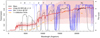 |
Fig. 2. Individual photometric filters (black) that make up the KV450 dataset. Each filter curve is shown as an overall transmission spectrum incorporating mirror, detector, and filter effects. We also show the typical transmission spectrum of the atmosphere at Paranal (blue) for modest values of precipitable water vapour (2.2 mm) and zenith angle (30°). In addition, we also show the median LE PHARE spectrum of all KV450 galaxies with photometric redshift ZB = 1.2 and magnitude r ∼ 24 (red). The 68th and 99th percentiles of these models are also shown as shaded red regions. The 1σ detection limits of each band (orange chevrons and dotted line, derived from the values in Table 1) are also shown, for reference. These model spectra demonstrate the complementarity of the KiDS & VIKING surveys; a typical galaxy at the furthest and faintest end of our analysis is still detected in all bands. It also demonstrates the main benefit of having NIR imaging within this dataset, in that it allows much more accurate constraint of photometric redshifts for (4000 Å) Balmer-break galaxies at redshifts z ≳ 1. |
The optical data for KV450 are reduced using the same reduction pipelines as in KiDS-450. Specifically, the ASTROWISE (Valentijn et al. 2007) pipeline is used for reducing the ugri-band images and measuring multi-band photometry for all sources. Independently, the THELI (Erben et al. 2005; Schirmer 2013) pipeline performs an additional reduction of the r-band data, which is used for cross-validating the ASTROWISE reduction and for performing shape measurements for weak lensing analyses.
The only difference between the KiDS-450 and KV450 optical datasets is that the KV450 optical reduction incorporates an updated photometric calibration. KiDS-450 invoked only relative calibration across the ugri-bands with stellar-locus-regression (SLR, High et al. 2009). The absolute calibration of these data was reliant on nightly standard star observations and the overlap between u- and r-band tiles to homogenise the photometry. Since the publication of Hildebrandt et al. (2017), the first data release from the European Space Agency’s Gaia mission has been made available (Gaia Collaboration 2016). Gaia offers a sufficiently homogeneous, well-calibrated anchor that can be used to greatly improve this absolute calibration. The calibration procedure is described in de Jong et al. (2017) and all optical data used here are absolutely calibrated in this way.
2.2. VIKING infrared data
VIKING is an imaging survey conducted with the Visible and InfraRed CAMera (VIRCAM) on ESO’s 4m VISTA telescope. The KiDS and VIKING surveys were designed together, with the specific purpose of providing well-matched optical and NIR data for ∼1350 square degrees of sky in the Galactic North and South. As such, the surveys share an almost identical footprint on-sky, with minor differences being introduced due to differences in the camera field of view and observation strategy. VIKING surveys these fields in five NIR bands (ZYJHKs), whose filter transmission curves are shown in Fig. 2, and total exposure times in each band are chosen such that the depths of KiDS and VIKING are complementary.
A detailed description of the VIKING survey design and observation strategy can be found in Edge et al. (2013) and Venemans et al. (2015). Briefly, VIRCAM consists of 16 individual HgCdTe detectors, each with a 0.2 × 0.2 square degree angular size, but which jointly span a ∼1.2 square degree field of view, thus leaving considerable gaps between each detector. Observations made by VIRCAM for VIKING therefore implement a complex dither pattern which is able to fill in the detector gaps while also performing jittered observations to enable reliable estimation of complex NIR backgrounds and sampling of data across detector defects. The observation strategy thus involves taking multiple exposures with small (i.e. much less than detector width) jitter steps, taken in quick succession, which are then stacked together to create a “paw-print”. The stacked paw-print still has large gaps between the 16 detectors, and so a dither pattern of six stacked paw-prints is required in order to create a contiguous ∼1.5 square degree image, called a tile. The reduction of the data, and the production of these individual data products (reduced exposures, stacked paw-prints, and completed tiles), is carried out by the Cambridge Astronomy Survey Unit (CASU, González-Fernández et al. 2018; Lewis et al. 2010). These reduced data are then transferred to the Edinburgh Royal Observatory Wide Field Astronomy Unit VISTA Science Archive (WFAU VSA, Irwin et al. 2004; Hambly et al. 2008; Cross et al. 2012) where they are benchmarked and stored.
Through the WFAU database, we are able to retrieve any of the three levels of data-product described above: exposures, paw-prints, and/or tiles. We opt to work with individual paw-print level data. This is mainly because the tile level data are frequently made up of paw-prints with a range of different point-spread functions (PSFs), and this can lead to complications later in our analysis (specifically regarding flux estimation; see Sect. 3). Therefore, we begin our combination of KiDS and VIKING by first downloading all the available stacked paw-prints from the WFAU. We then perform a recalibration of the individual paw-prints following the methodology of Driver et al. (2016) to correct the images for atmospheric extinction (τ) given the observation airmass (secχ), remove the exposure-time (t, in seconds) from the image units, and convert the images from various Vega zero-points (Zv) to a standard AB zero-point of 30 (using the documented Vega to AB correction factors, XAB; González-Fernández et al. 2018) which roughly translates to an image gain of ADU/e− = 1. The recalibration factor used is multiplicative, applied to all pixels in each detector image I:
 (1)
(1)
and is calculated as:
![Mathematical equation: $$ \begin{aligned} \log _{10}({\mathcal{F} }_{r}) =&-0.4\left[Z_{\rm v}-2.5\log _{10}(1/t)\right.\nonumber \\&\left.-\tau \left(\sec \chi -1\right)+X_{\rm AB}-30\right]. \end{aligned} $$](/articles/aa/full_html/2019/12/aa34879-18/aa34879-18-eq4.gif) (2)
(2)
This preprocessing of each VISTA detector also involves performing an additional background subtraction, which is done using the SWARP software (Bertin 2010) with a 256 × 256 pixel mesh size and 3 × 3 mesh filter for the bicubic spline. This allows the removal of small-scale variations in the NIR background with minimal impact on the source fluxes (Driver et al. 2016). Unlike GAMA, however, we do not recombine the individual paw-prints into tiles or large mosaics; we choose instead to work exclusively with the individual recalibrated detectors throughout our analysis.
After this processing, we perform a number of quality control tests to ensure that the imaging is sufficiently high quality for our flux analysis. In particular, we check distributions of background, seeing, recalibration factor (Eq. (2)), and number counts for anomalies. After these checks, we determined that a straight cut on the recalibration factor was sufficient to exclude outlier detectors, and thus implement the same rejection of detectors as in Driver et al. (2016); namely accepting only detectors with ℱr ≤ 5.0.
After this processing and quality control, we transfer the accepted imaging over to our flux measurement pipeline. Our final sample consists of 301 824 individual detectors across the five VIKING filters, drawn from the WFAU proprietary database v21.3, which are spread throughout the KiDS-450 footprint. This database, however, does not yet contain the full VIKING dataset, as reduction and ingestion of the final VIKING data (taken as recently as February 2018) is ongoing. As such, the final overlap between the KiDS footprint and VIKING is likely to continue to grow with future KiDS+VIKING data releases.
3. Photometry and photometric redshifts
3.1. 9-band photometry
Multi-band photometry is extracted from the combined KiDS+VIKING data using the Gaussian Aperture and PSF (GAaP; Kuij-ken 2008; Kuij-ken et al. 2015) algorithm. The algorithm generates PSF-corrected Gaussian-aperture photometry that is particularly well suited for colour-measurements which are used for estimating photometric redshift. The GAaP code differs to other standard photometric codes in that it does not require images to be pixel nor PSF matched in order to extract matched aperture fluxes (such as Source Extractor; Bertin & Arnouts 1996), and it limits flux estimation to the typically brighter and redder interior parts of galaxies, unlike codes designed for total flux photometry (such as LAMBDAR; Wright et al. 2016). GAaP also utilises purely Gaussian photometric apertures and PSFs (hence the name), and therefore performs the required image Gaussianisation prior to flux measurement.
The algorithm requires input source positions and aperture parameters, which we define by running Source Extractor (Bertin & Arnouts 1996) over our THELIr-band imaging in a so-called hot-mode. This refers specifically to the use of a low deblend threshold, which allows better deblending of small sources. This choice can have the adverse effect, however, of shredding large (often flocculant) galaxies. We choose this mode of extraction as we are mainly interested in sources in the redshift range 0.1 ≲ z ≲ 1.2, which are typically small and have smooth surface-brightness profiles. Once we have our extracted aperture parameters, the algorithm then performs a Gaussianisation of each measurement image. This removes systematic variation of the PSF over the image and allows for a more consistent estimate of source flux across the detector-plane. This Gaussianisation is performed by characterising the PSF over the input image using shapelets (Refregier 2003), and then fitting a smoothly varying spline to the shapelet distribution. For this reason, it is optimal to provide input images that do not have discrete changes in the shape of the PSF which cannot be captured by this smoothly varying distribution. The smooth function is then used to generate a kernel that, when convolved with the input image, normalises the PSF over the entire input image to a single Gaussian shape with arbitrary standard deviation.
Due to the requirement that the input imaging not have discrete changes in the PSF parameters, we require that the GAaP algorithm be run independently on subsets of the data that were taken roughly co-temporally. In the optical this is trivial; the 1.2 square degree stacks of jittered observations, called “pointings”, are always comprised of individual exposures with small offsets that were taken essentially cotemporally, due to the design of the detector array and survey observation strategy. This, combined with the stability of the PSF pattern across the field of view that is inherent to observations made at the Cassegrain focus of a Ritchey-Chrétien telescope, means that the stacked pointings are optimised for use in GAaP. Using the KiDS pointings for optical flux measurements with GAaP results in at most four flux estimates for any one KiDS source in the limited corner-overlap regions between adjacent pointings, or two flux estimates at the pointing edges. However, as in KiDS-450, we mask these overlap regions such that the final dataset contains only one measurement of all sources within the footprint, rather than performing a combination of these individual flux estimates. As such, our final flux and uncertainty estimates in the optical are simply those output directly by GAaP.
Conversely, the VISTA tiles are particularly sub-optimal for use in GAaP, due to the large dithers between successive paw-prints which are necessary to fill a contiguous area on-sky. Stacking such exposures with large dithering offsets can lead to significant discrete changes in the PSF of the stacked image, and this problem is exacerbated by the strong PSF variations over the focal plane inherent to observations made with such a fast telescope. Therefore, in order to streamline the data handling and avoid non-contiguous PSF patterns we decided to extract the VISTA NIR photometry from single VISTA detector images of individual paw-prints, as recommended in González-Fernández et al. (2018). In practice, the paw-print level data are provided as individual detector stacks, rather than as a mosaic of the telescope footprint.
Accordingly, we Gaussianise the PSF of each paw-print detector in the VIKING survey separately, and run GAaP on these units. As there is no one-to-one mapping between KiDS pointings and VIKING paw-prints, we are required to associate individual VIKING detectors with overlapping KiDS pointings on-the-fly. Furthermore, the VISTA dither pattern results in anywhere between one and six independent observations of a given source within the tile. This typically results in multiple flux measurements per source and band as most sky positions within the tile are covered by at least two paw-prints in the ZYHKs-bands and at least four paw-prints in the J-band. Therefore, for each source we calculate a final flux estimate, ff, that is the weighted average of the n individual flux measurements, fi:
 (3)
(3)
where the weight for each source is the individual GAaP measurement inverse variance  . The final flux uncertainty is the uncertainty on this weighted mean flux:
![Mathematical equation: $$ \begin{aligned} \sigma _{f_{\rm f}} = \left[\sum _{i=1}^n \sigma _{f_{i}}^{-2}\right]^{-\frac{1}{2}}\cdot \end{aligned} $$](/articles/aa/full_html/2019/12/aa34879-18/aa34879-18-eq7.gif) (4)
(4)
To test whether the GAaP flux uncertainties are suitable for use in estimating the final flux this way, we examine the distribution of sigma deviations between the final (weighted mean) flux and the individual estimates:
 (5)
(5)
where n is the number of flux measurements that went into the computation of ff and σff. In the limit where the individual flux uncertainties σfi are perfectly representative of the scatter between the individual measurements, the distribution of σΔi values should be a Gaussian with 0-mean and a standard deviation of 1. When the flux uncertainties are not representative of the scatter in the individual measurements, the distribution may deviate in mean, standard deviation, or both. In particular, systematic bias in the flux uncertainties as a function of flux will shift the mean of the distribution away from 0 (and/or give the distribution an obvious skewness), while over- or under-estimation of the uncertainties as a whole will cause the distribution standard deviation to decrease or increase, respectively. Figure 3 shows the distributions of σΔi for each of the five VIKING bands. The figure shows that our flux uncertainties in the ZYHKs-bands are appropriate and (for the vast majority of estimates) Gaussian; roughly 20% of our individual flux estimates have a scatter that is not well described by the simple final Gaussian uncertainty on our flux estimate, however this is not surprising given that the individual GAaP flux estimates are purely shot noise; they do not capture the full uncertainty in cases where there is considerable zero-point uncertainty, sky background, correlated noise, or other systematic effects which contribute to the flux uncertainty. Figure 3 also demonstrates that our flux uncertainties tend to be under-estimated in the J-band by roughly 30%. Encouragingly, however, the distributions show no sign of systematic bias in the flux uncertainties, which would be indicated by a significant skewness of these distributions.
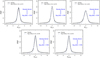 |
Fig. 3. Distributions of individual flux measurements with respect to the final flux estimate and uncertainty in KV450. Here we show per-band PDFs of σΔi, which demonstrates the accuracy of the final flux uncertainties for sources in KV450 (see text for details). We overlay on each distribution a Gaussian model that describes well the core of each distribution, providing the mean (μ), standard deviation (σ), and mixture fraction of the Gaussian given the total PDF (λ). We find that the final fluxes and uncertainties are generally a good description of the individual data, with typically > 70% of all individual (per-detector) flux estimates being well described by the simple Gaussian statistics. The wings of these distributions are caused by the existence of non-Gaussian noise components not encoded by the GAaP uncertainties (e.g. zero point uncertainties). We note that the J-band, however, has uncertainties that are underestimated by roughly 30%. Each panel is annotated with the kernel used in the PDF estimation, showing the width of the kernel and its log-bandwidth (bw). |
To verify the calibration of our imaging and flux estimates, we compare our estimates for a sample of KV450 stars to those measured by SDSS and/or 2MASS. Stars are particularly useful for this purpose as GAaP yields not only reliable colours but also total magnitudes for these sources (Kuij-ken et al. 2015), and therefore we need not be concerned with aperture effects in the flux comparisons. As the CASU pre-reduction assigns a photometric zeropoint to each VISTA paw-print based on a calibration with 2MASS, residuals in our multi-band photometry with 2MASS (particularly in the JHKs-bands) would indicate problems with our pipeline. Similar offsets with respect to SDSS in the Z-band would also be cause for concern. Hence these comparisons are used as quality control tests, typically on the level of a KiDS pointing. The distributions of the pointing-by-pointing offsets between our GAaP photometry and SDSS/2MASS are shown in Fig. 4, per band. The figure shows the PDFs of these residuals, as well as Gaussian fits to the distributions. In the Z-band, we have two lines: the solid line is a direct comparison to SDSS, while the dashed line is an extrapolation of 2MASS J − H colours to the Z-band. A similar extrapolation is shown in the Y-band. Both of these extrapolations have significant colour-corrections, and so should be taken somewhat cautiously. Encouragingly, however, in all the cases where we have fluxes that can be directly compared to one-another (i.e. in all but the Y-band), the direct comparison residuals are centred precisely on 0. Furthermore, in all cases the fluctuations between pointings are all within |Δm| < 0.02.
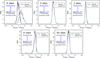 |
Fig. 4. Photometric comparison of KV450 stellar photometry in each of the ZYJHKs-bands to photometry from SDSS (for our Z-band only, shown as a solid line), and 2MASS in the ZYJHKs-bands. We note that as 2MASS does not cover the ZY-bands, comparisons there are made using an extrapolation based on the 2MASS J–H colour, as described in González-Fernández et al. (2018); these are shown here as dashed lines in the ZY comparison panels. We simultaneously fit these distributions with a single component Gaussian (blue), with the optimised fit parameters annotated. With the exception of the Y-band extrapolation (which has a 0.02 mag residual), all directly comparable fluxes are in perfect agreement. |
As a final test of the fidelity of our fluxes, we compare colours of KV450 stars with the same measured in 2MASS, to demonstrate that our observed colours are consistent with, but less noisy than, those from 2MASS. The distributions of KV450 and 2MASS J − H and H − Ks colours can be seen in Fig. 5. As expected, the KV450 colours show considerably less scatter, suggesting that they are a better representation of the underlying, intrinsic stellar colour distribution (Wright et al. 2016), and are therefore superior to the colours of 2MASS.
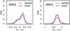 |
Fig. 5. Comparison between the colours of KV450 stars and the same sources measured by 2MASS. The reduction in scatter of the distribution indicates that the KV450 NIR data have significantly reduced uncertainties. |
Now confident that our fluxes are appropriate, we can further verify the appropriateness of our sample definition and effective-area calculations by comparing our measured galaxy number counts (in our extraction band, r) with previous works from the literature. Figure 6 shows the r-band number counts for the KV450 dataset compared to the compendium of survey number counts presented in Driver et al. (2016). We show the KV450 dataset both with and without the removal of stellar sources described in Sect. 4.2. Furthermore, we show the number counts for the sample of lensing sources used for cosmological inference (Hildebrandt et al. 2019). The lensing subset is constructed of sources which are suitable for shape measurement as described in detail in Hildebrandt et al. (2017). This lensing sample consists of 13.1 million sources, all of which fall within the r-band magnitude range 20 ≲ mr ≲ 25, are unblended, and are resolved.
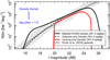 |
Fig. 6. r-band number counts for sources in KV450 before (solid black) and after (dotted black) removal of stars, and for the lensing sample (red). Each of these datasets is presented as raw number density; the number counts divided by the area of the sample (indicated in the legend), without any additional weighting. We compare these to the galaxy number counts from the literature compendium presented in Driver et al. (2016). The grey region shows the scatter in the data from their literature compendium, while the solid grey line traces the median of their compendium. Our number counts are in good agreement with the literature, although at the bright end our hot-mode source extraction leads to a dearth of the brightest galaxies (causing the dashed black line to begin to fall downwards at magnitudes brighter than r ∼ 19.5). |
We see that the all-galaxy sample is lacking in number counts at the brightest magnitudes; we attribute this to our hot-mode source extraction biasing against the extraction of the largest, brightest galaxies, as has been noted previously in earlier KiDS datasets (see, e.g., Tortora et al. 2018). Otherwise, the observed counts of both the all-galaxy- and lensing-only-samples are in excellent agreement with the literature compendium of r-band counts from Driver et al. (2016), suggesting that our sample definitions and area calculations are appropriate.
Unlike KiDS-450, we also require the final lensing sample to have full 9-band photometric coverage; successful photometric measurements are required for every source in all 9 bands. Table 2 provides the photometric measurement statistics for the lensing sample in KV450, as a function of individual band and for combinations of bands. The statistics shown are the fraction of sources with successful GAaP measurements (fgood) in all nine bands, for all sources that fall both within the area of mutual KiDS+VIKING coverage.
Measurement statistics for 13.09 million lensing sources that remain after all non-photometry KV450 masks have been applied, per band and as successive bands are added.
The table demonstrates that GAaP returns a successful flux measurement for greater than 98% of all lensing sources in all bands. However, as the failures are different in each band, the full sample ends up with successful estimates in all 9-bands for greater than 96% of would-be lensing sources. Therefore, the requirement of a successful GAaP measurement acts to trim our final lensing sample down by less than 4%. Furthermore, the lensing sample has significant detections in all 9-bands for over 66% of the full sample, and for over 69% of sources that have no GAaP failures (i.e. where there is data in all 9-bands). We note, however, that the u-band has the lowest number of significant detections within the dataset, by a considerable margin, but that this is mainly a reflection of physics rather than of the imaging depth. The rapidly declining nature of galaxy SEDs in this wavelength range at all redshifts, conspiring with the lower sensitivity of the band compared to, say, the g-band, means that the u-band experiences significantly more non-detected sources than any other band over our redshift window. Explained differently: the i-band, for example, sees no such dearth in detections despite being shallower than the u-band, courtesy of its probing a typically more luminous part of the galaxy SED (at z ≲ 1 this is primarily because of the flux increase associated with the 4000 Å break). Removing the u-band from our considerations of detection statistics, we find that we have significant detections in the griZYJHKs-bands for 82% of lensing sources in the dataset. This is a vindication of the combined KiDS+VIKING survey design, whereby limiting magnitudes were designed specifically with the goal of sampling the 9-band SEDs of the r-band selected KiDS sample.
For completeness, we investigate the cause of the GAaP failures in our dataset. These typically occur when either there are data missing, or when the algorithm is unable to compute the measurement aperture given the image PSF. The latter can occur when the PSF full-widths at half-maximum (FWHM) of the measurement image is considerably larger than the input (detection) aperture (Kuij-ken et al. 2015). As such, the input aperture size can be a source of systematic bias in the GAaP flux measurement procedure, as smaller input apertures are more likely to hit the aperture-PSF limit in one of our non-detection bands. We conclude, however, that this is unlikely to introduce significant biases into our subsequent analyses as less than 1.2% of sources per-band are affected by the GAaP measurement failure. Nonetheless, in future releases of KiDS+VIKING data, a recursive flux measurement method will be invoked, whereby sources that fail in any band due to this effect are subsequently re-measured with an artificially expanded GAaP input aperture.
After applying the requirement of successful (i.e. fgood) 9-band photometric estimation, we finish with a final lensing sample of ∼12.6 million sources, which are drawn from an effective area of 341.3 deg2 (see Sect. 2). This is a slight reduction in the effective area from KiDS-450 (360.3 deg2), however this area will recover somewhat in future KiDS+VIKING releases, as the final (full) VIKING area is processed and released by CASU (see Sect. 2.2).
3.2. Photometric redshifts
Photometric redshifts are estimated from the 9-band photometry using the public Bayesian Photometric Redshift (BPZ; Benítez 2000) code. We use the re-calibrated template set of Capak (2004) in combination with the Bayesian redshift prior from Raichoor et al. (2014); hereafter R14. We utilise the maximum amount of photometric information per source, providing BPZ with both flux estimates and limits (where available). Finally, input fluxes are extinction corrected before use within the BPZ code, using Schlegel et al. (1998) dust maps and per-band absorption coefficients.
We test the accuracy of our KiDS+VIKING photo-z estimates using a large sample of spectroscopic redshifts collected from a number of different surveys: zCOSMOS (Lilly et al. 2009), DEEP2 Redshift Survey (Newman et al. 2013), VIMOS VLT Deep Survey (Le Fèvre et al. 2013), GAMA-G15Deep (Kafle et al. 2018), and ESO-GOODS (Popesso et al. 2009; Balestra et al. 2010; Vanzella et al. 2008). This combined spectroscopic calibration sample, matched to KV450, includes > 33 000 sources extending over a 95% r-band magnitude quantile range of r ∈ [19.76, 24.75]. Within the sample, 96% of sources have full 9-band photometric information returned by GAaP, and 77% have significant detections in all 9-bands. This sample is therefore a reasonable match to the full KV450 dataset, which extends slightly deeper (r ∈ [20.82, 25.18]) and has 96% and 67% coverage and detection fractions, respectively (see Table 2). Detailed information on the collation of this spectroscopic calibration sample can be found in Hildebrandt et al. (2019).
We note here that, importantly, our testing and quality verification of the photo-z extend only to the maximum likelihood point-estimate values returned from the redshift fitting code: the ZB values. This is because for the analyses performed with the photo-z within KiDS, only the point-estimates are ever used; the full photo-z PDFs are never considered. Therefore, we note here for clarity that the statistics presented here all extend to the ZB values only, and no quality testing of the full photo-z PDFs is presented.
Figure 7 shows a comparison of our photo-z with the spectroscopic calibration sample. The figure shows the standard photo-z vs. spec-z distributions for three separate photo-z realisations, as well as annotated statistics for each distribution as a function of photo-z. These statistics are calculated using the distribution of (zB − zspec)/(1 + zspec)≡Δz/(1 + z) values, and are: the normalised median-absolute-deviation of Δz/(1 + z) (σm); the fraction of sources with |Δz/(1 + z)| > 3σm (η3); and the fraction of sources with |Δz/(1 + z)| > 0.15 (ζ0.15). The three photo-z realisations include the initial KiDS-450 4-band photo-z as presented in Hildebrandt et al. (2017), an updated version of the 4-band photo-z using the R14 prior, and KiDS+VIKING 9-band photo-z (also with the R14 prior). Comparing the two 4-band photo-z setups, we see that the R14 prior is effective in suppressing outliers in the low photo-z portion of the distribution by over 30%, but shows worse performance at the highest redshifts, where the outlier rate and scatter increase by factors of 1.14 and 1.13 respectively. The 9-band photo-z, however, shows significant improvement over both 4-band setups. In particular, the inclusion of the NIR data allows us to constrain photo-z in the zB > 0.9 range (σm = 0.096) to almost the same level of precision as for the zB < 0.9 sample (σm = 0.061), an extremely powerful addition to the dataset, particularly for studies of cosmic-shear where these data carry a very strong signal. We note that the value of η3 increases slightly for the high-z portion of the 9-band dataset, however this is mainly because the value of σm here is reduced by nearly a factor of two; the higher σm in the 4-band cases conceals the non-Gaussianity of the distributions, artificially reducing the value of η3 there.
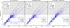 |
Fig. 7. Photometric redshifts (zB) vs. spectroscopic redshifts (zspec) in the deep calibration fields. Left: original KiDS-450 photo-z based on ugri-band photometry. Middle: improved ugri-band photo-z based on the Bayesian prior by Raichoor et al. (2014). Right: KV450 photo-z based on ugriZYJHKs photometry as well as the improved prior. The grey region of the figures indicate sources beyond the zB limit imposed in the KiDS-450 analysis. Annotated in each panel is: the normalised median-absolute-deviation (σm) of the quantity (zB − zspec)/(1 + zspec)≡Δz/(1 + z), the fraction of sources with |Δz/(1 + z)| > 3σm (η3), and the fraction of sources with |Δz/(1 + z)| > 0.15 (ζ0.15). Each of these quantities is calculated individually for the sources above and below zB = 0.9. The value of σm is also displayed graphically in each panel using the black dotted lines. We note the significant improvement in all quantities that is seen when moving from the 4- to 9-band photometry, and in particular that we are now able to constrain zB > 0.9 sources to almost the same accuracy as those zB < 0.9 in the original KiDS-450 dataset. |
We can further motivate the importance of having NIR data for computation of photo-z by exploring how the statistics which describe the photo-z vs. spec-z distribution vary under the addition of NIR data, as a function of spec-z. We note though, that these statistics as a function of spec-z cannot be used for the quantification of photo-z performance for sources selected in discrete bins of photometric redshift (such as tomographic cosmic shear bins). Rather, these can be used exclusively to demonstrate the influence the additional wavelength information has on the data as a function of true redshift.
Figure 8 shows the change in our three parameters of interest as a function of zspec, for changes in the prior (for the 4-band KiDS-450 data in grey) and under addition of NIR data (using only the R14 prior in colours). The three parameters in the figure are as follows: σm, the median bias in Δz/(1 + z) (μΔz), and ζ0.15. Each parameter is shown using a running median in 20 equal-N bins of zspec. The equivalent figure with bins constructed as a function of zB and r-magnitude are given in Figs. 9 and 10.
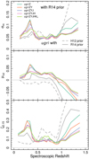 |
Fig. 8. Variation in the photo-z vs. spec-z distribution parameters as a function of spec-z, for the 4-band KiDS-450 dataset with two different priors (grey lines), and as a function of NIR photometric information for the KV450 dataset (coloured lines). The three panels show the spread in the distribution, determined by a running normalised-median-absolute-deviation from the median (σm; top), the median bias in the photo-z distribution (μΔz; middle), and the fraction of sources with |Δz|/(1 + zspec) > 0.15 (ζ0.15; bottom). The addition of the Raichoor et al. (2014) prior to the 4-band data causes significantly better behaviour at low zB, while the addition of NIR data improves the population consistency and scatter in particular at high zB. The same properties as a function of photo-z and magnitude are given in Figs. 9 and 10. |
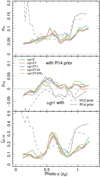 |
Fig. 9. Variation in the photo-z vs. spec-z distribution parameters as a function of photo-z. The figure is constructed the same as Fig. 8. |
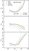 |
Fig. 10. Variation in the photo-z vs. spec-z distribution parameters as a function of r-magnitude. The figure is constructed the same as Fig. 8. |
The statistics as a function of zspec demonstrate that it is the combination of all 9-bands which performs the best across both the full gambit of statistics and the redshift baseline. The addition of the Z-band causes a clear improvement, in all statistics, over the 4-band case when we move beyond zspec = 0.9. This is because at zspec = 0.9 4000 Å-break flux enters the i-band, and in the 4-band case is therefore poorly sampled and becomes sensitive to noise fluctuations. With the addition of the Z-band, however, sampling of this flux is more robust and the statistics unilaterally improve. There are further improvements with the addition of subsequent bands: the Y-band causes a large reduction in scatter at z > 1, because the same post-4000 Å-break flux is now sampled by two or more bands (further decreasing the influence of noise). This benefit then saturates (subsequent bands do not improve the high zspec scatter), however the story nonetheless continues. The J- and H-bands are primarily responsible for a reduction of outliers at 0.2 < zspec < 0.4, where a model degeneracy (which is considerably worse after the inclusion of the Z-band) populates a cloud which can be seen in the photo-z–spec-z distribution (Fig. 7). Finally the Ks-band helps bring the low-zspec scatter down further, and also produces the lowest overall high-zspec outlier rate. Indeed, the outlier rate at z > 0.9 reduces continuously with the number of bands added. For these reasons, we conclude that the full complement of the 9-band data is what is required for the best performance, especially at zspec > 0.9.
3.2.1. Binned by zB
Again, we note that these trends shown above and in Fig. 8 are not directly transferable to a sample defined as a function of photo-z. We show the influence of the individual bands on photometrically defined samples in Fig. 9.
Looking at the effect of the updated prior on the 4-band photo-z statistics, we see that the new prior has the effect of greatly reducing scatter at low zB, while also reducing bias across essentially all zB. There is also a slight increase in the outlier rate with the new prior at intermediate and high zB, but this is minor compared to the significant decrease at zB < 0.4.
When combining the NIR data (starting with the Z-band) with the 4-band photometry, we see an immediate improvement in the distribution scatter and outlier rate at high zB > 0.7. In this range, when incorporating all NIR bands, we see decreases in scatter of between 30 and 60%, over the 4-band R14-prior case. Of particular note is the effect of adding the NIR-bands to the outlier rate at zB > 0.7. Here the added data reduce the observed outlier rate by a factor of ∼2. Overall, the distributions demonstrate that NIR data as a whole are extremely useful in constraining photo-z for sources in the redshift range 0.7 < zB < 0.9, and are invaluable for the estimation of photo-z at zB > 0.9.
3.2.2. Binned by r-magnitude
The introduction of the NIR data actually creates an increase in the observed scatter and outlier rate for sources at the brightest magnitudes. However beyond r = 22, both the scatter and outlier rate reduce to levels superior to the 4-band data. With the addition of subsequent NIR bands (i.e. YJHKs), we see a essentially continual improvement in all statistics over the whole magnitude range. Otherwise, the distributions show the expected behaviour of photo-z accuracy as a function of noise; the fainter (and so noisier) data exhibit higher scatter in their photo-z and similarly higher outlier rates. We note, though, that this definition of outlier rate becomes somewhat nonsensical beyond r ∼ 25, where the scatter of the distribution reaches ∼0.15 (i.e. the outlier criterion).
Of particular interest is the reduction in bias that is seen with the introduction of the J-band at r ≳ 23. The sources here show the largest bias in the 4-band case, and this bias is only partially reduced in the Z and Y band cases. However the introduction of the J-band data causes the bias to reduce somewhat. The addition of the H- and Ks-bands do not further reduce the scatter at the faint end, however do produce slightly lower biases at the brightest magnitudes. Again, we therefore conclude that the combined 9-band dataset is therefore that which provides the best overall statistics.
3.2.3. Photo-z distributions per field
Another quality check for the homogeneity of the data is to compare the distributions of photometric redshift in each of our five fields (shown in Fig. 1). We compare the distribution of all photo-z estimates for sources within our lensing sample (Fig. 6) with r ≤ 23.5. These two cuts allow us to compare the photo-z distributions per field for samples of known non-stellar sources in a regime agnostic to the effects of variable depth from the comparison; a like-for-like comparison. These distributions per field are shown in Fig. 11. We can see from the distribution that the fields are in very good agreement, with only GS appearing slightly deeper than the other four fields. As such, we conclude that the photo-z among the different KV450 fields demonstrate satisfactory homogeneity.
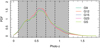 |
Fig. 11. Distributions of photo-z within each of our five survey fields (shown in Fig. 1). The figure shows the PDF estimated using a width = 0.1 top-hat kernel for each of the five fields (coloured lines). The tomographic bins used in KiDS are shown by the grey shading and black dashed lines. Sources plotted here are those within the KV450 lensing selection (Fig. 6) and with an additional r ≤ 23.5 magnitude selection, to remove the effect of variable depth on the comparison. The figure demonstrates that, in a like-for-like comparison between the fields, the KV450 photo-z are homogeneous. |
4. Higher-order data products
We can subsequently utilise our photo-z estimates to derive higher-order data-products. For this work, we choose to explore the rest-frame photometric properties of a selection of KV450 sources, as well as examine the fidelity of integrated properties, namely stellar masses. In order to explore these properties we perform template-fitting to the broad-band spectral energy distributions (SEDs) of each KV450 source, while maintaining a fixed redshift at the value of zB.
4.1. SED fitting
To estimate the rest-frame properties of our KV450 sources, we perform SED fitting with the LE PHARE (Arnouts et al. 1999; Ilbert et al. 2006) template-fitting code, using a standard concordance cosmology of Ωm = 0.3, ΩΛ = 0.7, H0 = 70 km s−1 Mpc−1, Chabrier (2003) IMF, Calzetti et al. (1994) dust-extinction law, Bruzual & Charlot (2003) stellar population synthesis (SPS) models, and exponentially declining star formation histories. Input photometry to LE PHARE is as described in Sect. 3, including the per-band extinction corrections as used in BPZ. We fix the source redshift to be the value of zB returned from BPZ. We opt to fit SEDs to all > 45 million KV450 sources, regardless of masking, so that any and all subsequent subsamples of KV450 data may incorporate our stellar mass estimates. This requires that we also allow SEDs to be fit with QSO and stellar templates, for which we use the internal LE PHARE defaults.
4.2. Star-galaxy separation
One advantage of fitting all photometric sources in this way is that we are able to use the higher-order data products to assist with star-galaxy separation. In particular, by fitting all sources with templates for QSOs, stars, and galaxies, we are able to identify stellar contaminants that otherwise would make it into our overall sample. To do this, we identify all sources that are best fit by a stellar template in LE PHARE and which have an angular extent that is point-like; specifically a flux-radius of 0.8 arcseconds or smaller. Using this simple cut, we are able to produce an exceptionally clean galaxy-only sample (as shown in Fig. 6). We note, however, that this rejection has no effect on the lensing sample as the high-fidelity point-source rejection that is already performed during shape-fitting is very effective at removing stellar contaminants. Indeed, all sources that are identified as stars using our SED based selection are also flagged as stars during shape-fitting. Furthermore, for the sources with g ≤ 21, we can cross-reference our stellar classification with that from the Gaia DR2 (Gaia Collaboration 2018) point-source catalogue. Comparing to Gaia we find that 99.1% of our sources classified as stars (and which are brighter than the g ≤ 21 Gaia magnitude limit) are also classified as stars by Gaia3. Again, this further increases our confidence in the stellar classification possible using our SED products.
4.3. Stellar mass estimates
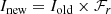
For this work, we are primarily interested in assessing the fidelity of stellar masses that are estimated using the KV450 dataset. Our stellar masses, estimated by LE PHARE, are calculated as the mass of stars required to produce the observed galaxy SED given the best-fit stellar population, assuming the combination of models given in Sect. 4.1. Therefore, in order to recover a fair estimate of the galaxy stellar mass, the observed SED must be representative of the total light emitted from the galaxy. Our aperture fluxes, however, have been intentionally optimised for high-fidelity colours, rather than for the recovery of total fluxes. This means that our mass estimates here will be systematically below what would be recovered with a total flux aperture, mainly as a function of source size. In order to remedy this systematic effect, we opt to use our quasi-total Source Extractor AUTO flux estimates (measured during our initial source extraction) to correct our masses. To do this, we implement a correction akin to the fluxscale correction discussed in Taylor et al. (2011), Wright et al. (2017), although the implementation there was designed to correct for systematic bias in Kron (1980) apertures for changing galaxy profile shapes.
Here our fluxscale factor, ℱ, is a multiplicative correction defined as the linear ratio of the quasi-total Source Extractor r-band AUTO flux to the non-total GAaP r-band flux: ℱ = fAUTO/fGAaP. This correction is applied post-facto to the LE PHARE stellar mass estimates. The correction devised is such that our final SEDs will be fixed to the AUTO flux estimate, and our SEDs themselves will be reflective of the flux contained within the GAaP apertures. This can lead to systematic biases. For example, if there are significant colour gradients within the galaxies in our sample, such that the colours within and beyond our apertures differ considerably, then our SEDs will tend to be non-representative of the true integrated galaxy spectrum. Admittedly, however, this is only likely to be a significant effect for galaxies whose size is significantly larger than the PSF; specfically low-redshift galaxies for which our analysis pipeline is already sub-optimal.
For validation purposes, we compare our fluxscale-corrected stellar mass estimates to those also estimated by GAMA (Wright et al. 2017) and G10-COSMOS (Andrews et al. 2017; Driver et al. 2018) in Fig. 12. Both of these studies utilise spectroscopic redshifts, and implement the same cosmology, SPS models, dust-law, and IMF as used in this work when estimating stellar masses. They also use total matched aperture fluxes. These similarities allow direct comparison of our mass estimates, despite the use of different algorithms and wavelength bandpasses for the mass estimation. We perform this comparison both for the KV450 masses described above and for masses estimated in the same way but utilising only 4-band photometric information (i.e. the KiDS-450 equivalent masses). The GAMA dataset here is sky-matched to our KiDS-450 and KV450 datasets within a 1 arcsec radius, for GAMA galaxies with redshift z ≥ 0.004, GAMA redshift quality flag nQ > 2, and for KiDS sources with zB < 0.7 (so as to avoid spurious matches to the much deeper KiDS-450 and KV450 catalogues). The G10-COSMOS sample is subset such that it contains only sources with spectroscopic redshifts (i.e. those with G10-COSMOS flag zuse ≤ 3) and is also sky-matched to KiDS with a 1 arcsecond radius. We note that there is no requirement for consistency between matched sources photo-z and spec-z values. As such, the scatter here is a reflection of the scatter in the mass estimates due to, jointly, systematics in our photometric data and photo-z estimation.
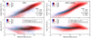 |
Fig. 12. Comparison between stellar mass estimates from both KiDS-450 (left) and KV450 (right) with those from both the GAMA and G10-COSMOS samples, for those sources which overlap. KiDS-450 masses here are derived using the KiDS-450 photo-z (i.e. with H12 prior) and only ugri photometry. Both KiDS datasets are shown with masses which have been corrected using our fluxscale parameter. Sources in the comparison samples are selected for comparison only if their masses have been estimated using spectroscopic redshifts. The figure demonstrates the significant improvement in mass estimates that is made when using 9-band photometric information and, in particular, significant reduction on the scatter of the deep G10-COSMOS dataset. Scatter in the highest-mass GAMA sources is due to the updated photo-z prior, which is optimised for sources fainter than many high-mass GAMA galaxies. |
We see that the KiDS-450 masses show significant scatter in the comparison distributions (Fig. 12, left panels), particularly for the COSMOS dataset which extends to significantly higher redshift than the GAMA sample (σ = 0.464). Conversely, we see very good agreement with the same sample when using masses derived with KV450; σ = 0.202. We note that the scatter in the mass comparison with the GAMA sample increases slightly when moving from KiDS-450 to KV450. This increase in scatter between masses estimated in KV450 and by GAMA is slightly larger than the typical scatter induced by slightly different mass estimation methods (∼0.2 dex; see Wright et al. 2017, for a detailed discussion of such comparisons and systematic effects), and is induced by the updated photo-z prior implemented here (Sect. 3.2). This is not surprising, given that this prior is optimised for analysis of the full KiDS sample, which is COSMOS-like. The variation between KV450 and GAMA is highly correlated with systematic differences between the GAMA spec-z and KV450 photo-z, which shows roughly a factor of two stronger bias than we see in the main survey spectroscopic calibration sample (i.e. Fig. 7), again due largely to our updated prior. Importantly, we see no such systematic variations in our comparisons with G10-COSMOS (in mass or photo-z) for KV450. This is in stark contrast to the significant bias and scatter that is evident in the KiDS-450 to G10-COSMOS comparisons. In particular, we note that the bias in the G10-COSMOS comparison decreases by nearly an order of magnitude when moving from KiDS-450 (μΔ = −0.213) to KV450 (μΔ = 0.041). Furthermore, we note that the scatter in the comparison between KV450 and G10-COSMOS is reduced to σΔ = 0.208; consistent with the 0.2 dex typical uncertainty induced by different mass estimation methods agnostic of variations in input photometry and redshifts. As such, we conclude that, for our KV450 sample, the 9-band stellar mass estimates are equivalent in quality to those that can be estimated using significantly more accurate spectroscopic redshift surveys.
5. Stellar mass function
Given the accuracy of our observed stellar mass estimates when compared to the G10-COSMOS survey, we are prompted to explore whether we can reproduce complex redshift-dependent mass functions using these estimates. Such mass functions typically require spectroscopic redshift estimates and/or high-accuracy photo-z estimates derived from 20+ broad and narrow photometric bands (see, e.g., Andrews et al. 2017; Davidzon et al. 2017; Wright et al. 2018). However, given the apparent fidelity of our mass and photo-z estimates, we wish to explore whether we can derive sensible mass-evolution distributions from our relatively low-resolution photo-z estimates alone.
Fluxscale-corrected stellar masses from LE PHARE are shown in Fig. 13 for all galaxies in the KV450 footprint, as a function of zB. The distribution shows an underdensity of high-mass sources at low-redshift, and also a considerable amount of structure as sources approach the detection limit. This structure is a form of redshift focussing, and is caused by sources systematically dropping below the detection limit in particular bands as a function of galaxy SED shape. Otherwise, the distribution is well bounded and fairly uniform, showing little evidence of photo-z dependent biases.
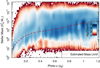 |
Fig. 13. Distribution of all KV450 galaxy stellar mass estimates as a function of photo-z. The data is shown as a 2D-histogram with logarithmic scaling. The distribution is fairly consistent with what is expected of a magnitude limited galaxy sample, although the incompleteness at low-z is worth noting. The distribution is fairly uniform above the mass limits (red dashed line). Below the limits we see signs of systematic incompleteness and redshift focussing (caused by the typically noisier data there). |
We wish to use this distribution of stellar masses to estimate a series of volume-complete galaxy stellar mass functions (GSMFs) for the KV450 dataset. To do this, we first define the mass limit of the dataset as a function of photo-z. We take the same method of estimating the mass limits as described in Wright et al. (2017), using the turn-over points in both number counts and photo-z to estimate the mass-completeness limit. Briefly, the mass limits as a function of photo-z are constructed assuming that any observed down-turn in number-density is due exclusively to incompleteness; that the mass function, over the redshifts and masses probed here, has no true down-turn. Using this assumption we estimate the completeness limit as a function of photo-z as being the point at which either comoving number density and/or stellar mass number density starts to fall. The procedure is shown graphically in Fig. C1 of Wright et al. (2017). The calculation of the completeness limit is done in a series of overlapping bins of photo-z and stellar mass, and the resulting limit estimates are fit with a fifth-order polynomial. This derived mass limit is shown in Fig. 13 as a dashed red line. The mass limit can be seen to effectively select against sources in the redshift-focused (low signal-to-noise ratio) portions of the distribution, and suggests that the mass estimates of KV450 can be considered to be volume complete down to M⋆ ≥ 1010 M⊙ for sources with zB ≤ 1.
Using these mass limits, we define a series of volume-complete bins in stellar mass and redshift, and calculate the resulting mass functions in these bins. These are shown in Fig. 14. For our binning, we choose to use the same tomographic redshift limits as are implemented in our cosmological analysis (Hildebrandt et al. 2019), out to zB = 1.2. The mass functions are calculated using a simple volume calculated using the survey area and the redshift limits annotated in each bin, and we show the mass functions derived with and without the implementation of the fluxscale correction, for reference. For comparison, we also show the model evolutionary mass functions presented in Wright et al. (2018), derived using a compilation of consistently analysed GAMA, G10-COSMOS, and 3D-HST data over the redshift range 0.1 ≤ z ≤ 5. For demonstration, the Wright et al. (2018) model is shown both as the model expectation at the mean redshift of the bin (grey line), and as the range of model values (grey shading) that would be expected when allowing for: photo-z bias |ΔzB|≤0.2, additional systematic bias in our stellar mass estimation (|ΔM⋆, sys|≤0.2 dex), and Eddington bias (|ΔM⋆, edd|=0.2 dex).
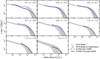 |
Fig. 14. Galaxy stellar mass functions for the KV450 dataset, shown with (blue, solid) and without (blue, dashed) the fluxscale factor incorporated, compared to the mass function model given in Wright et al. (2018) (dark grey). KV450 lines are shown only over the range where we believe the mass function to be volume complete. To ensure a fair comparison, we also show the model mass function when allowing for uncertainty in photometric redshift (|Δz|≤0.02) and Eddington bias (|ΔM⋆|≤0.2) in grey. The KV450 mass function shows a significant deviation from the expectation in the lowest redshift bin, which we attribute to a bias against selecting the largest-angular-size galaxies in our analysis (see Sect. 5). In all other bins the agreement with the model is exceptional given the simplicity of the analysis performed, and inspires considerable confidence in the fidelity of our mass estimates. |
The first photo-z bin shows a mass function that has a clear deficit in number density for the highest mass sources. This deficit, we argue, is again caused by our pipelines optimisation for small-angular scale sources: the largest sources on sky will also be the most massive at low redshift, and our analysis methods are biased against accurate extraction of these sources. In the subsequent bins, however, the mass functions from our sample are in good agreement with the evolutionary model of Wright et al. (2018). This is particularly noteworthy, given the coarseness of our photo-z estimation and that no correction for the redshift distribution bias (such as is done in cosmic shear analyses; see Hildebrandt et al. 2017) has been attempted. The mass functions, however, clearly suffer from considerable Eddington bias in their masses (i.e. our mass functions are biased towards higher masses).
6. Summary
In this work we present a new photometric dataset for astrophysics and cosmology, KiDS+VIKING-450. The dataset builds on the optical dataset of KiDS-450 with the inclusion of 5-band NIR data from the VIKING survey, reduced and analysed in a way entirely consistent with the optical dataset.
We discuss the reduction of the VIKING dataset, and the derivation of relevant data products such as photometry. We demonstrate that the products derived are robust, consistent with, and superior to previous photometric estimates of sources from overlapping surveys such as 2MASS.
Using our photometry, we derive new 9-band photometric redshifts for the full KV450 sample, and compare these new photo-z to those presented previously in Hildebrandt et al. (2017). We find that the new photo-z exhibit a reduced scatter in Δz/(1 + z) (especially at high photo-z; down by ∼40% compared to the ugri-only case), a lower overall bias (down 50%), and allow us to dramatically improve our ability to accurately estimate photo-z beyond zB = 0.9, with the outlier rate reducing by over 40%. The improvement is sufficiently dramatic as to motivate the inclusion of a higher-redshift bin in KiDS cosmic shear studies using this dataset (Hildebrandt et al. 2019), and to motivate us to explore whether our photo-z alone are able to be used to constrain galaxy evolution parameters of interest (such as the stellar mass function) out to high redshift.
Using the SED fitting code LE PHARE, we estimate stellar masses for all sources in the KV450 footprint. We compare these mass estimates to previous samples from GAMA (Wright et al. 2017) and G10-COSMOS (Andrews et al. 2017), finding good agreement between the datasets. Our comparison to G10-COSMOS (a sample that matches the overall KV450 dataset well) demonstrates negligible bias in our mass estimates (μΔ = 0.041) and a scatter that is equivalent to that seen inherent to stellar mass estimates agnostic of changes to photometry and redshift (σΔ = 0.202; Wright et al. 2017; Taylor et al. 2011). Furthermore, we demonstrate that the SED fits allow us to perform a high-fidelity star-galaxy separation, and thereby clean the full sample of contaminating sources.
Using our mass estimates, we calculate the mass-completeness limit of the dataset, deriving an empirical mass limit that suggests the sample is volume complete above M⋆ ≥ 1010 M⊙ at zB ≤ 1. We bin the data into eight volume complete samples spanning 0.1 ≤ zB ≤ 2 and plot the resulting galaxy stellar mass functions for these bins. Comparing these bins to the evolutionary model of the GSMF from Wright et al. (2018), we find agreement in the range of 0.3 ≤ zB ≤ 2. The lowest photo-z bin shows considerable incompleteness at high-masses, which we attribute to our extraction pipeline being optimised for small-angular-size sources. In the regime where our pipeline is optimised, we demonstrate that we are able to reproduce the results of previous studies which utilised spectroscopic redshifts and/or significantly more photometric data than we use here. Future KiDS+VIKING releases, containing three times the on-sky area utilised here, will further push the boundaries of studies that are possible with photometric-only data.
There are a number of pointings, particularly at the survey edges, which have only slight overlap between KiDS and VIKING. This causes the overall loss in area (∼19 deg2) to be somewhat larger than the loss of only seven full pointings would suggest.
Should the Gaia catalogue have contamination by truly-extended galaxies, this would indicate a galaxy contamination within our star sample in the same proportion.
Acknowledgments
This work is been supported by European Research Council Consolidator Grants: 770935 (AHW, HH) and 647112 (CH). HH is also supported by Emmy Noether (Hi 1495/2-1) and Heisenberg grants (Hi 1495/5-1) of the Deutsche Forschungsgemeinschaft. KK acknowledges support by the Alexander von Humboldt Foundation. CH acknowledges support from the Max Planck Society and the Alexander von Humboldt Foundation in the framework of the Max Planck-Humboldt Research Award endowed by the Federal Ministry of Education and Research. AC acknowledges support from NASA grant 15-WFIRST15-0008. JTAdJ is supported by the Netherlands Organisation for Scientific Research (NWO) through grant 621.016.402. ACE acknowledges support from STFC grant ST/P00541/1. This work is supported by the Deutsche Forschungsgemeinschaft in the framework of the TR33 “The Dark Universe”. Based on observations made with ESO Telescopes at the La Silla Paranal Observatory under programme IDs 179.A-2004, 177.A-3016, 177.A-3017, 177.A-3018, 298.A-5015. This work was performed in part at Aspen Center for Physics, which is supported by National Science Foundation grant PHY-1607611. All authors contributed to the development and writing of this paper. The authorship list is given in three groups: the lead authors (AHW, HH, KK), followed by two alphabetical groups. The first alphabetical group includes those who are key contributors to both the scientific analysis and the data products. The second group covers those who have either made a significant contribution to the data products or to the scientific analysis.
References
- Abbott, T., Abdalla, F. B., Allam, S., et al. 2016, Phys. Rev. D, 94, 022001 [NASA ADS] [CrossRef] [Google Scholar]
- Aihara, H., Arimoto, N., Armstrong, R., et al. 2018, PASJ, 70, S4 [NASA ADS] [Google Scholar]
- Amendola, L., Appleby, S., Avgoustidis, A., et al. 2018, Liv. Rev. Relativ., 21, 2 [Google Scholar]
- Andrews, S. K., Driver, S. P., Davies, L. J. M., et al. 2017, MNRAS, 464, 1569 [NASA ADS] [CrossRef] [Google Scholar]
- Arnaboldi, M., Neeser, M. J., Parker, L. C., et al. 2007, The Messenger, 127, 28 [NASA ADS] [Google Scholar]
- Arnouts, S., Cristiani, S., Moscardini, L., et al. 1999, MNRAS, 310, 540 [NASA ADS] [CrossRef] [Google Scholar]
- Bacon, D. J., Refregier, A. R., & Ellis, R. S. 2000, MNRAS, 318, 625 [NASA ADS] [CrossRef] [Google Scholar]
- Balestra, I., Mainieri, V., Popesso, P., et al. 2010, A&A, 512, A12 [NASA ADS] [CrossRef] [EDP Sciences] [Google Scholar]
- Banerji, M., Jouvel, S., Lin, H., et al. 2015, MNRAS, 446, 2523 [NASA ADS] [CrossRef] [Google Scholar]
- Becker, M. R., Troxel, M. A., MacCrann, N., et al. 2016, Phys. Rev. D, 94, 022002 [NASA ADS] [CrossRef] [Google Scholar]
- Benítez, N. 2000, ApJ, 536, 571 [NASA ADS] [CrossRef] [Google Scholar]
- Bertin, E. 2010, Astrophysics Source Code Library [record ascl:1010.068] [Google Scholar]
- Bertin, E., & Arnouts, S. 1996, A&AS, 117, 393 [NASA ADS] [CrossRef] [EDP Sciences] [Google Scholar]
- Bolzonella, M., Miralles, J. M., & Pelló, R. 2000, A&A, 363, 476 [NASA ADS] [Google Scholar]
- Brammer, G. B., van Dokkum, P. G., & Coppi, P. 2008, ApJ, 686, 1503 [NASA ADS] [CrossRef] [Google Scholar]
- Bruzual, G., & Charlot, S. 2003, MNRAS, 344, 1000 [NASA ADS] [CrossRef] [Google Scholar]
- Buchs, R., Davis, C., Gruen, D., et al. 2019, MNRAS, 489, 820 [NASA ADS] [CrossRef] [Google Scholar]
- Calzetti, D., Kinney, A. L., & Storchi-Bergmann, T. 1994, ApJ, 429, 582 [NASA ADS] [CrossRef] [Google Scholar]
- Capak, P. L. 2004, PhD Thesis, University of Hawai’i [Google Scholar]
- Chabrier, G. 2003, PASP, 115, 763 [NASA ADS] [CrossRef] [Google Scholar]
- Cross, N. J. G., Collins, R. S., Mann, R. G., et al. 2012, A&A, 548, A119 [NASA ADS] [CrossRef] [EDP Sciences] [Google Scholar]
- Davidzon, I., Ilbert, O., Laigle, C., et al. 2017, A&A, 605, A70 [NASA ADS] [CrossRef] [EDP Sciences] [Google Scholar]
- de Jong, J. T. A., Verdoes Kleijn, G. A., Boxhoorn, D. R., et al. 2015, A&A, 582, A62 [NASA ADS] [CrossRef] [EDP Sciences] [Google Scholar]
- de Jong, J. T. A., Verdois Kleijn, G. A., Erben, T., et al. 2017, A&A, 604, A134 [NASA ADS] [CrossRef] [EDP Sciences] [Google Scholar]
- Driver, S. P., Hill, D. T., Kelvin, L. S., et al. 2011, MNRAS, 413, 971 [NASA ADS] [CrossRef] [Google Scholar]
- Driver, S. P., Wright, A. H., Andrews, S. K., et al. 2016, MNRAS, 455, 3911 [NASA ADS] [CrossRef] [Google Scholar]
- Driver, S. P., Andrews, S. K., da Cunha, E., et al. 2018, MNRAS, 475, 2891 [NASA ADS] [CrossRef] [Google Scholar]
- Edge, A., Sutherland, W., Kuijken, K., et al. 2013, The Messenger, 154, 32 [NASA ADS] [Google Scholar]
- Erben, T., Schirmer, M., Dietrich, J. P., et al. 2005, Astron. Nachr., 326, 432 [NASA ADS] [CrossRef] [Google Scholar]
- Gaia Collaboration (Brown, A. G. A., et al.) 2016, A&A, 595, A2 [NASA ADS] [CrossRef] [EDP Sciences] [Google Scholar]
- Gaia Collaboration (Brown, A. G. A., et al.) 2018, A&A, 616, A1 [NASA ADS] [CrossRef] [EDP Sciences] [Google Scholar]
- González-Fernández, C., Hodgkin, S. T., Irwin, M. J., et al. 2018, MNRAS, 474, 5459 [NASA ADS] [CrossRef] [Google Scholar]
- Hambly, N. C., Collins, R. S., Cross, N. J. G., et al. 2008, MNRAS, 384, 637 [NASA ADS] [CrossRef] [Google Scholar]
- High, F. W., Stubbs, C. W., Rest, A., Stalder, B., & Challis, P. 2009, AJ, 138, 110 [NASA ADS] [CrossRef] [Google Scholar]
- Hikage, C., Oguri, M., Hamana, T., et al. 2019, PASJ, 71, 43 [NASA ADS] [CrossRef] [Google Scholar]
- Hildebrandt, H., Arnouts, S., Capak, P., et al. 2010, A&A, 523, A31 [NASA ADS] [CrossRef] [EDP Sciences] [Google Scholar]
- Hildebrandt, H., Choi, A., Heymans, C., et al. 2016, MNRAS, 463, 635 [NASA ADS] [CrossRef] [Google Scholar]
- Hildebrandt, H., Viola, M., Heymans, C., et al. 2017, MNRAS, 465, 1454 [Google Scholar]
- Hildebrandt, H., Köhlinger, F., van den Busch, J. L., et al. 2019, A&A, in press, https://doi.org/10.1051/0004-6361/201834878 [Google Scholar]
- Ilbert, O., Arnouts, S., McCracken, H. J., et al. 2006, A&A, 457, 841 [NASA ADS] [CrossRef] [EDP Sciences] [Google Scholar]
- Ilbert, O., Capak, P., Salvato, M., et al. 2009, ApJ, 690, 1236 [NASA ADS] [CrossRef] [Google Scholar]
- Irwin, M. J., Lewis, J., Hodgkin, S., et al. 2004, in Optimizing Scientific Return for Astronomy through Information Technologies, eds. P. J. Quinn, & A. Bridger, Proc. SPIE, 5493, 411 [Google Scholar]
- Jee, M. J., Tyson, J. A., Hilbert, S., et al. 2016, ApJ, 824, 77 [NASA ADS] [CrossRef] [Google Scholar]
- Joachimi, B., Cacciato, M., Kitching, T. D., et al. 2015, Space Sci. Rev., 193, 1 [NASA ADS] [CrossRef] [Google Scholar]
- Kafle, P. R., Robotham, A. S. G., Driver, S. P., et al. 2018, MNRAS, 479, 3746 [NASA ADS] [CrossRef] [Google Scholar]
- Kron, R. G. 1980, ApJS, 43, 305 [NASA ADS] [CrossRef] [Google Scholar]
- Kuij-ken, K. 2008, A&A, 482, 1053 [NASA ADS] [CrossRef] [EDP Sciences] [Google Scholar]
- Kuij-ken, K., Heymans, C., Hildebrandt, H., et al. 2015, MNRAS, 454, 3500 [NASA ADS] [CrossRef] [Google Scholar]
- Laigle, C., Davidzon, I., Ilbert, O., et al. 2019, MNRAS, 486, 5104 [NASA ADS] [CrossRef] [Google Scholar]
- Le Fèvre, O., Cassata, P., Cucciati, O., et al. 2013, A&A, 559, A14 [NASA ADS] [CrossRef] [EDP Sciences] [Google Scholar]
- Lewis, J. R., Irwin, M., & Bunclark, P. 2010, in Astronomical Data Analysis Software and Systems XIX, eds. Y. Mizumoto, K. I. Morita, & M. Ohishi, ASP Conf. Ser., 434, 91 [NASA ADS] [Google Scholar]
- Lilly, S. J., Le Brun, V., Maier, C., et al. 2009, ApJS, 184, 218 [Google Scholar]
- Mandelbaum, R. 2018, ARA&A, 56, 393 [NASA ADS] [CrossRef] [Google Scholar]
- Massey, R., Heymans, C., Bergé, J., et al. 2007, MNRAS, 376, 13 [NASA ADS] [CrossRef] [Google Scholar]
- Newman, J. A., Cooper, M. C., Davis, M., et al. 2013, ApJS, 208, 5 [Google Scholar]
- Planck Collaboration VI. 2019, A&A, submitted [arXiv:1807.06209] [Google Scholar]
- Popesso, P., Dickinson, M., Nonino, M., et al. 2009, A&A, 494, 443 [NASA ADS] [CrossRef] [EDP Sciences] [Google Scholar]
- Raichoor, A., Mei, S., Erben, T., et al. 2014, ApJ, 797, 102 [NASA ADS] [CrossRef] [Google Scholar]
- Refregier, A. 2003, MNRAS, 338, 35 [NASA ADS] [CrossRef] [Google Scholar]
- Rhodes, J., Refregier, A., & Groth, E. J. 2001, ApJ, 552, L85 [NASA ADS] [CrossRef] [Google Scholar]
- Schirmer, M. 2013, ApJS, 209, 21 [NASA ADS] [CrossRef] [Google Scholar]
- Schlegel, D. J., Finkbeiner, D. P., & Davis, M. 1998, ApJ, 500, 525 [NASA ADS] [CrossRef] [Google Scholar]
- Taylor, E. N., Hopkins, A. M., Baldry, I. K., et al. 2011, MNRAS, 418, 1587 [NASA ADS] [CrossRef] [Google Scholar]
- Tortora, C., Napolitano, N. R., Spavone, M., et al. 2018, MNRAS, 481, 4728 [NASA ADS] [CrossRef] [Google Scholar]
- Troxel, M. A., Krause, E., Chang, C., et al. 2018, MNRAS, 479, 4998 [NASA ADS] [CrossRef] [Google Scholar]
- Valentijn, E. A., McFarland, J. P., Snigula, J., et al. 2007, in Astronomical Data Analysis Software and Systems XVI, eds. R. A. Shaw, F. Hill, & D. J. Bell, ASP Conf. Ser., 376, 491 [NASA ADS] [Google Scholar]
- Van Waerbeke, L., Mellier, Y., Erben, T., et al. 2000, A&A, 358, 30 [NASA ADS] [Google Scholar]
- Vanzella, E., Cristiani, S., Dickinson, M., et al. 2008, A&A, 478, 83 [NASA ADS] [CrossRef] [EDP Sciences] [Google Scholar]
- Venemans, B. P., Verdoes Kleijn, G. A., Mwebaze, J., et al. 2015, MNRAS, 453, 2259 [NASA ADS] [CrossRef] [Google Scholar]
- Wittman, D. M., Tyson, J. A., Kirkman, D., Dell’Antonio, I., & Bernstein, G. 2000, Nature, 405, 143 [NASA ADS] [CrossRef] [PubMed] [Google Scholar]
- Wright, A. H., Robotham, A. S. G., Bourne, N., et al. 2016, MNRAS, 460, 765 [NASA ADS] [CrossRef] [Google Scholar]
- Wright, A. H., Robotham, A. S. G., Driver, S. P., et al. 2017, MNRAS, 470, 283 [NASA ADS] [CrossRef] [Google Scholar]
- Wright, A. H., Driver, S. P., & Robotham, A. S. G. 2018, MNRAS, 480, 3491 [NASA ADS] [CrossRef] [Google Scholar]
All Tables
Magnitude limits and typical seeing values for each of the KiDS+VIKING photometric bands.
Measurement statistics for 13.09 million lensing sources that remain after all non-photometry KV450 masks have been applied, per band and as successive bands are added.
All Figures
|
Fig. 1. Footprint of the post-masking KiDS-450 dataset. Top: distribution of the KiDS-450 fields on-sky, relative to the Ecliptic and Galactic planes. The Galactic plane is plotted with a width of 20°, which roughly traces the observed width of the Galaxy thick disk. Lower panels: each of the individually named KiDS-450 patches (on their own scale). The points in each patch show the distribution of KiDS-450 photometric sources that remain after applying the bright-star mask. Points are coloured according to their overall observational coverage: green points have full KiDS+VIKING optical and NIR coverage, blue points have full KiDS optical coverage but only partial VIKING NIR coverage, and orange points have KiDS optical coverage only. As such the green and blue data show the footprint of the full KiDS+VIKING-450 (KV450) sample. |
| In the text | |
|
Fig. 2. Individual photometric filters (black) that make up the KV450 dataset. Each filter curve is shown as an overall transmission spectrum incorporating mirror, detector, and filter effects. We also show the typical transmission spectrum of the atmosphere at Paranal (blue) for modest values of precipitable water vapour (2.2 mm) and zenith angle (30°). In addition, we also show the median LE PHARE spectrum of all KV450 galaxies with photometric redshift ZB = 1.2 and magnitude r ∼ 24 (red). The 68th and 99th percentiles of these models are also shown as shaded red regions. The 1σ detection limits of each band (orange chevrons and dotted line, derived from the values in Table 1) are also shown, for reference. These model spectra demonstrate the complementarity of the KiDS & VIKING surveys; a typical galaxy at the furthest and faintest end of our analysis is still detected in all bands. It also demonstrates the main benefit of having NIR imaging within this dataset, in that it allows much more accurate constraint of photometric redshifts for (4000 Å) Balmer-break galaxies at redshifts z ≳ 1. |
| In the text | |
|
Fig. 3. Distributions of individual flux measurements with respect to the final flux estimate and uncertainty in KV450. Here we show per-band PDFs of σΔi, which demonstrates the accuracy of the final flux uncertainties for sources in KV450 (see text for details). We overlay on each distribution a Gaussian model that describes well the core of each distribution, providing the mean (μ), standard deviation (σ), and mixture fraction of the Gaussian given the total PDF (λ). We find that the final fluxes and uncertainties are generally a good description of the individual data, with typically > 70% of all individual (per-detector) flux estimates being well described by the simple Gaussian statistics. The wings of these distributions are caused by the existence of non-Gaussian noise components not encoded by the GAaP uncertainties (e.g. zero point uncertainties). We note that the J-band, however, has uncertainties that are underestimated by roughly 30%. Each panel is annotated with the kernel used in the PDF estimation, showing the width of the kernel and its log-bandwidth (bw). |
| In the text | |
|
Fig. 4. Photometric comparison of KV450 stellar photometry in each of the ZYJHKs-bands to photometry from SDSS (for our Z-band only, shown as a solid line), and 2MASS in the ZYJHKs-bands. We note that as 2MASS does not cover the ZY-bands, comparisons there are made using an extrapolation based on the 2MASS J–H colour, as described in González-Fernández et al. (2018); these are shown here as dashed lines in the ZY comparison panels. We simultaneously fit these distributions with a single component Gaussian (blue), with the optimised fit parameters annotated. With the exception of the Y-band extrapolation (which has a 0.02 mag residual), all directly comparable fluxes are in perfect agreement. |
| In the text | |
|
Fig. 5. Comparison between the colours of KV450 stars and the same sources measured by 2MASS. The reduction in scatter of the distribution indicates that the KV450 NIR data have significantly reduced uncertainties. |
| In the text | |
|
Fig. 6. r-band number counts for sources in KV450 before (solid black) and after (dotted black) removal of stars, and for the lensing sample (red). Each of these datasets is presented as raw number density; the number counts divided by the area of the sample (indicated in the legend), without any additional weighting. We compare these to the galaxy number counts from the literature compendium presented in Driver et al. (2016). The grey region shows the scatter in the data from their literature compendium, while the solid grey line traces the median of their compendium. Our number counts are in good agreement with the literature, although at the bright end our hot-mode source extraction leads to a dearth of the brightest galaxies (causing the dashed black line to begin to fall downwards at magnitudes brighter than r ∼ 19.5). |
| In the text | |
|
Fig. 7. Photometric redshifts (zB) vs. spectroscopic redshifts (zspec) in the deep calibration fields. Left: original KiDS-450 photo-z based on ugri-band photometry. Middle: improved ugri-band photo-z based on the Bayesian prior by Raichoor et al. (2014). Right: KV450 photo-z based on ugriZYJHKs photometry as well as the improved prior. The grey region of the figures indicate sources beyond the zB limit imposed in the KiDS-450 analysis. Annotated in each panel is: the normalised median-absolute-deviation (σm) of the quantity (zB − zspec)/(1 + zspec)≡Δz/(1 + z), the fraction of sources with |Δz/(1 + z)| > 3σm (η3), and the fraction of sources with |Δz/(1 + z)| > 0.15 (ζ0.15). Each of these quantities is calculated individually for the sources above and below zB = 0.9. The value of σm is also displayed graphically in each panel using the black dotted lines. We note the significant improvement in all quantities that is seen when moving from the 4- to 9-band photometry, and in particular that we are now able to constrain zB > 0.9 sources to almost the same accuracy as those zB < 0.9 in the original KiDS-450 dataset. |
| In the text | |
|
Fig. 8. Variation in the photo-z vs. spec-z distribution parameters as a function of spec-z, for the 4-band KiDS-450 dataset with two different priors (grey lines), and as a function of NIR photometric information for the KV450 dataset (coloured lines). The three panels show the spread in the distribution, determined by a running normalised-median-absolute-deviation from the median (σm; top), the median bias in the photo-z distribution (μΔz; middle), and the fraction of sources with |Δz|/(1 + zspec) > 0.15 (ζ0.15; bottom). The addition of the Raichoor et al. (2014) prior to the 4-band data causes significantly better behaviour at low zB, while the addition of NIR data improves the population consistency and scatter in particular at high zB. The same properties as a function of photo-z and magnitude are given in Figs. 9 and 10. |
| In the text | |
|
Fig. 9. Variation in the photo-z vs. spec-z distribution parameters as a function of photo-z. The figure is constructed the same as Fig. 8. |
| In the text | |
|
Fig. 10. Variation in the photo-z vs. spec-z distribution parameters as a function of r-magnitude. The figure is constructed the same as Fig. 8. |
| In the text | |
|
Fig. 11. Distributions of photo-z within each of our five survey fields (shown in Fig. 1). The figure shows the PDF estimated using a width = 0.1 top-hat kernel for each of the five fields (coloured lines). The tomographic bins used in KiDS are shown by the grey shading and black dashed lines. Sources plotted here are those within the KV450 lensing selection (Fig. 6) and with an additional r ≤ 23.5 magnitude selection, to remove the effect of variable depth on the comparison. The figure demonstrates that, in a like-for-like comparison between the fields, the KV450 photo-z are homogeneous. |
| In the text | |
|
Fig. 12. Comparison between stellar mass estimates from both KiDS-450 (left) and KV450 (right) with those from both the GAMA and G10-COSMOS samples, for those sources which overlap. KiDS-450 masses here are derived using the KiDS-450 photo-z (i.e. with H12 prior) and only ugri photometry. Both KiDS datasets are shown with masses which have been corrected using our fluxscale parameter. Sources in the comparison samples are selected for comparison only if their masses have been estimated using spectroscopic redshifts. The figure demonstrates the significant improvement in mass estimates that is made when using 9-band photometric information and, in particular, significant reduction on the scatter of the deep G10-COSMOS dataset. Scatter in the highest-mass GAMA sources is due to the updated photo-z prior, which is optimised for sources fainter than many high-mass GAMA galaxies. |
| In the text | |
|
Fig. 13. Distribution of all KV450 galaxy stellar mass estimates as a function of photo-z. The data is shown as a 2D-histogram with logarithmic scaling. The distribution is fairly consistent with what is expected of a magnitude limited galaxy sample, although the incompleteness at low-z is worth noting. The distribution is fairly uniform above the mass limits (red dashed line). Below the limits we see signs of systematic incompleteness and redshift focussing (caused by the typically noisier data there). |
| In the text | |
|
Fig. 14. Galaxy stellar mass functions for the KV450 dataset, shown with (blue, solid) and without (blue, dashed) the fluxscale factor incorporated, compared to the mass function model given in Wright et al. (2018) (dark grey). KV450 lines are shown only over the range where we believe the mass function to be volume complete. To ensure a fair comparison, we also show the model mass function when allowing for uncertainty in photometric redshift (|Δz|≤0.02) and Eddington bias (|ΔM⋆|≤0.2) in grey. The KV450 mass function shows a significant deviation from the expectation in the lowest redshift bin, which we attribute to a bias against selecting the largest-angular-size galaxies in our analysis (see Sect. 5). In all other bins the agreement with the model is exceptional given the simplicity of the analysis performed, and inspires considerable confidence in the fidelity of our mass estimates. |
| In the text | |
Current usage metrics show cumulative count of Article Views (full-text article views including HTML views, PDF and ePub downloads, according to the available data) and Abstracts Views on Vision4Press platform.
Data correspond to usage on the plateform after 2015. The current usage metrics is available 48-96 hours after online publication and is updated daily on week days.
Initial download of the metrics may take a while.