© ESO 2019

1. Introduction

In the last decade, all large astronomical facilities operating at centimetre, millimetre, and sub-millimetre wavelengths have continuously increased their sensitivity and instantaneous observing bandwidth, dramatically enhancing their potential scientific output. As examples of current bandwidth capabilities, the SMA now records instantaneously 32 GHz, NOEMA 15.4 GHz, IRAM 30 m 15.6 GHz, and VLA 8 GHz. While ALMA currently records 8 GHz, it is planned to increase the bandwidth up to 16 GHz in the coming years¹. Future planned facilities also target wide instantaneous frequency coverage, such as the Next Generation VLA (ngVLA), expected to cover 20 GHz² and the SKA 5 GHz³.

The large bandwidths together with the superb sensitivities provided by both the new interferometric facilities and single-dish telescopes equipped with multi-beam receivers result in extremely large three-dimensional spectroscopic data cubes. Such data sets contain huge amounts of physical, kinematic, and chemical information on molecular and atomic recombination lines. This wealth of information allows us to study the physical conditions and the chemical processes taking place in a wide variety of astronomical objects, ranging from solar system objects and protoplanetary disks to galaxies observed in the early Universe.

While the instrumental capabilities have been improving, the tools to analyse the extremely rich and complex datasets are still in their infancy. Using different strategies, during the last decade a number of tools have been developed in parallel for spectral line identification and molecular emission analysis at different levels. Here we briefly describe the tools available to date together with their key functionalities to serve as a comparison among them and with SLIM/MADCUBA as described below:

WEEDS⁴ (Maret et al. 2011), developed in FORTRAN within the GILDAS⁵ package, provides tools for the visualisation of simulated molecular line profiles using the local thermodynamical equilibrium (LTE) approximation superimposed on the observed single-pointing spectra.

CASSIS⁶, developed in Java, is a stand-alone package containing a molecular line catalogue which is included in Herschel Interactive Processing Environment⁷ (HIPE) as a plug-in⁸. It preforms both the LTE and the non-LTE analysis for single-pointing spectra. For the LTE analysis, CASSIS simulates the expected LTE molecular line profiles and visualises them on the observed spectra while relevant parameters can be manually adjusted. CASSIS provides the LTE parameters and their associated errors derived by a non-linear least-squares fit to the data. For the non-LTE analysis, CASSIS connects to the large velocity gradient (LVG) code RADEX⁹ (van der Tak et al. 2007) when collisional cross sections for the molecular species are available, providing the H₂ densities and the molecular column densities for an assumed kinetic temperature.

XCLASS¹⁰ (Möller et al. 2017), mainly developed in FORTRAN, can be executed within CASA¹¹ (McMullin et al. 2007) and performs the LTE line profile simulation and the non-linear least-squares fit to the data from both single pointing spectra and 3D spectroscopic data cubes. It allows to a very complex distribution of molecular and continuum slabs (clouds) along the line of sight, considering the effects of the molecular line attenuation by foreground dust and the molecular line absorption of the background continuum. This tool runs with python scripts using input files and delivers the results of fitted LTE parameters and their associated errors.

With the advent of ALMA and its objective of providing science-ready data products, molecular astrophysics and astrochemistry are now becoming unique and very powerful tools within the grasp of non-experts in radio/(sub)millimetre astronomy and molecular astrophysics. In the past, the analysis of the molecular data was based on a number of approximations helping to simplify the derivation of physical conditions and molecular abundances from very limited set of data. Usually these approximations have a limited range of applicability and in many cases provide degenerated results. Thanks to current facilities such as ALMA, it is now possible to choose the appropriate set of molecular transitions that when combined with suited tools will not require the user to rely on such strong approximations. This combination allows the user to better constrain the physical parameters by removing some of the degeneracies.

Newly developed analysis tools must also meet the challenging requirement of being intuitive and easy to use while easily and efficiently handling large volumes of data. The MAdrid Data CUBe Analysis package (MADCUBA), developed at the Centro de Astrobiología (CSIC, INTA), was designed with two basic premises in mind: efficiency (required to handle large and complex data sets) and ease of use, thanks to user-friendly intuitive interfaces for non-experts on molecular astrophysics.

In this paper we present and briefly describe the main data handling functionalities of MADCUBA. In summary, and for the sake of comparison with the existing tools described above, MADCUBA allows interactive manipulation of single-pointing spectra and spectroscopic data cubes with a number of functions working in both spatial and spectroscopic axes. The SLIM package at the core of MADCUBA provides spectral analysis tools for modelling molecular emission. Here, we provide details on the formalism used by SLIM, where the equations, approximations, and limitations are comprehensively described. The SLIM package provides molecular and recombination line identification tools as well as LTE molecular analysis for emission and absorption lines for both single-pointing spectra and spectroscopic data cubes. A background continuum source can be added to produce absorption profiles, but attenuation by dust is not yet implemented. Such analysis tools are not yet available for recombination lines within SLIM. However, both the dust attenuation and the recombination line modelling will be implemented in the future. The generation of synthetic LTE molecular spectra is fully interactive through sliders allowing users to change the input physical parameters, with on-the-fly visualisation of the resulting model spectra overlaid on the observed data or data cubes. In addition, SLIM provides tools to automatically fit physical parameters with their associated errors derived from non-linear least-squares fit to the data.

MADCUBA has already been used in recent years in many papers addressing different scientific topics in a variety of astronomical sources: prestellar cores (Jiménez-Serra et al. 2016), infrared-dark clouds (Cosentino et al. 2018), low-mass star-forming regions (Martín-Doménech et al. 2017; Rivilla et al. 2019a), high-mass star-forming regions (Rivilla et al. 2016, 2017a,b; Rizzo et al. 2017; Zahorecz et al. 2017; Colzi et al. 2018; Moscadelli et al. 2018; Beltrán et al. 2018), Galactic centre giant molecular clouds (Zeng et al. 2018; Rivilla et al. 2018, 2019b; Riquelme et al. 2018) and HII regions (Armijos-Abendaño et al. 2018), and external galaxies (Martín et al. 2014, 2015, 2019; Aladro et al. 2015; Harada et al. 2018; Sewiło et al. 2018).

The paper is organised as follows: In Sect. 2 we enumerate the main cube handling functionalities of MADCUBA. In Sect. 3 we describe in detail the SLIM tool and present the spectroscopic database, the basic radiative transfer formulation, and the assumptions made to generate synthectic molecular spectra in LTE. We also explain the automatic non-linear least-squares fitting algorithm, and discuss the derived errors associated to the fitted LTE parameters and the quality of the fit. We present a number of examples to illustrate the potential of SLIM. To go beyond a mere presentation of the radiative transfer LTE formulation, in Sect. 4, we discuss common approximations used in the literature to analyse molecular spectra and point out the limitations and degeneracies of such approximations. Building on this discussion, we describe how MADCUBA can facilitate the estimation of uncertainties derived from these degeneracies.

2. MAdrid Data CUBe Analysis package

MADCUBA¹² is a package developed to import, visualise, manipulate, process, and analyse molecular and recombination line astronomical data from both 3D spectroscopic cubes and single-pointing spectra. It was designed to combine a user-friendly interface and a powerful visualisation and data-analysis system able to deal with large volumes of data. MADCUBA provides simple tools to analyse and interpret molecular and recombination line spectroscopic observations. It is a stand-alone package developed in Java¹³ as a plug-in for ImageJ¹⁴ (Schneider et al. 2012; Schindelin et al. 2015). ImageJ is a Java-based highly extensible open-source image-processing program developed by the U.S. National Institutes for Health for the analysis of scientific multidimensional images mainly in Biology. ImageJ provides the core infrastruture for the visualisation and processing of data cubes, and the framework for interactive scripting. Additionally, MADCUBA makes use of the STIL¹⁵, non-tam-fits¹⁶, and skyview Libraries¹⁷. The STIL library is used for managing large tables, non-tam-fits is a Java library for reading and writing FITS (Flexible Image Transport System) files, and Skyview provides the spatial World Coordinate System infrastructure.

MADCUBA is an out-of-the box¹⁸ toolkit with no other requirements than Java 1.8 or above. It can be downloaded from the MADCUBA website¹² and does not require installation. After decompressing the downloaded file, it can be run directly from the executable files within the MADCUBA directory. It is compatible with Linux, Mac OS X, and Windows environments. The package can be easily updated to the latest version by replacing two .jar files that can be independently downloaded from the website.

2.1. Importing data into MADCUBA

MADCUBA can read and import data from the main radio to far-infrared (FIR) observatories in the world (i.e. ALMA, Herschel, NOEMA, SMA, VLA, GBT, IRAM 30 m, Effelsberg 100 m). The native data format for both data cubes and spectra is FITS. MADCUBA can import single spectra and data cubes in FITS format generated by CASA, GBT-IDL, or MIRIAD. Herschel products (versions 2, 2.5 and 3) from the Herschel Science Archive¹⁹ for the three instruments (PACS, SPIRE, and HIFI) and GILDAS single spectra (a working local GILDAS installation is required), and GILDAS data cubes (previously exported to FITS) can also be imported. In addition, MADCUBA offers a generic data cube import option, able to deal with a large variety of data cubes parameters, as well as the possibility of importing spectra from a plain formatted ASCII file (see Appendix B.1 for a sample input file).

2.2. Visualisation and handling of data cubes and spectra

MADCUBA uses the powerful infrastructure offered by ImageJ to interactively visualise and handle astronomical data cubes and spectra through a graphical user interface (GUI). MADCUBA allows interactive visualisation of single and multiple data cubes and spectra. Figure 1 shows a screenshot with a sample MADCUBA session where its main windows are displayed and identified.

Fig. 1. Screenshot showing the use of MADCUBA to spatially synchronise multiple datacubes. In this case, eight ALMA datacubes taken from the data published by Martín et al. (2019) are loaded and synchronised. From top to bottom and left to right, the windows shown are: the main ImageJ window; the main MADCUBA menu; the cube container window displaying the currently opened data cubes; the synchronise cube window listing the data cubes currently synchronised (in this case all opened ones); the cube display where the selected channel of the first opened data cube is displayed and the RoI is interactively defined (black contour on image); and finally the eight spectra corresponding to the integrated spectra from the RoI for each synchronised datacube. We note that the image channel displayed is selected with a red line in the top left spectrum, which corresponds to the spectrum from the cube displayed.

The spectral visualisation offers the possibility to interactively convert both the spectral and intensity axes to the most commonly used units in radio, millimetre (mm), sub-mm, and FIR astronomy (see Appendix A). The visualisation allows the user to merge and/or overlay multiple spectra in a single plot when the spectral axis is set to frequency, wavelengths, or energy.

The cube visualisation is achieved by on-the-fly displaying the image plane at the selected spectral channel in the cube, and plotting the spectrum from the selected spatial pixel(s) in the image plane. The latter includes the possibility to show the integrated spectrum over a spatial region of interest (RoI) defined on the image as a rectangle, ellipse, polygon, or line. Similarly to other common visualisation packages such as ds9²⁰ (Joye & Mandel 2003), RoIs can be defined on the image with different geometries (rectangle, ellipse, polygon, or line). The definition of RoI can be performed either interactively or through command line scripting (Sect. 2.3). The defined RoI is recorded in the cube history file and, like ds9, it can be loaded onto the image from the ImageJ scripting window. The cube visualisation also allows to change spectral and intensity units and to choose between equatorial and Galactic coordinates. The spectrum in the plot can be extracted and saved for further analysis. The intensity or flux units and the solid angle corresponding to the selected RoI of the extracted spectra are calculated and saved to the spectra accordingly. These parameters will be used for modelling within SLIM (Sect. 3).

In addition to single cube visualisation, MADCUBA allows spatially synchronised visualisation of multiple cubes. The pixel or RoI selected in a cube is propagated to all the synchronised cubes in celestial coordinates. The propagated RoIs are displayed on the images of all synchronised cubes and the corresponding spatially integrated spectra are plotted (see Fig. 1). The synchronised multiple spectra from all the cubes can also be extracted and saved for further analysis with SLIM (Sect. 3). This is particularly handy for spectral line surveys carried out via multiple frequency tunings or even a simple ALMA project whose products will contain multiple cubes of individual spectral windows.

MADCUBA also offers a number of tools for data-cube and spectra manipulation such as spectral baseline for cubes and single spectrum, spatial, and spectroscopic smoothing and cropping, spectral interpolation and re-sampling, Gaussian fits to line profiles, and velocity- or frequency-integrated images from cubes. Cropping and smoothing can also be applied simultaneously to synchronised data cubes.

2.3. Scripting and history file

ImageJ contains a plethora of contributed scripts and plug-ins, and allows for user-scripting in Jython²¹. MADCUBA makes use of the infrastructure of the Macro/scripting language (IJM²²) built into ImageJ that allows many aspects of MADCUBA and ImageJ to be controlled. Most of the functions and tools in MADCUBA can be used in scripts as a sequence of actions to manipulate large data sets of cubes and spectra in an automatic way (see Appendix B.2 for a sample script). Scripts can be easily written in MADCUBA since the operations performed by the user can be recorded automatically. The recorded scripts can then be edited and tested interactively to apply the same operations to other data sets. Frequently used scripts can be installed in MADCUBA to be used as tools, and they can also be distributed to other users.

The MADCUBA product is composed of two files, the data file and the history file. The history file contains all the operations performed to the data and is written in the scripting language. This file allows all the operations performed on the data to easily be tracked and repeated and also allows the user to edit the parameters used in the data processing.

3. Spectral line identification and modelling

The SLIM package is a key module of MADCUBA for the analysis of spectra (Fig. 2). The SLIM tools allow line identification of spectroscopic features through queries to its spectroscopic database (Sect. 3.1) which can be overlaid on top of the displayed spectra. It also provides the infrastructure to model the molecular emission (Sect. 3.2) and to generate synthetic spectra from input physical parameters (Sect. 3.3). These synthetic spectra can be overlaid on top of the observed spectra and/or fitted to the observations in order to derive the best fit to the physical parameters with their corresponding uncertainties (Sect. 3.4). An extension of this tool to automatically analyse data cubes is under development.

Fig. 2. Screenshot showing the use of SLIM within MADCUBA to identify and fit a synthetic LTE model to an observed broadband spectrum. In this case, a 30 000 channel ALMA spectrum is displayed where more than 100 molecular species have been fitted. From top to bottom and left to right, the windows shown are: the main ImageJ window; the main MADCUBA menu; the modelling tab within the SLIM tool with the list of fitted species and the sliders in the bottom to interactively adjust the physical parameters; the spectra container window displaying the currently opened spectra; the plot showing the full spectrum with the transitions of the selected species labeled; the SLIM PLOT showing the synthetic model overlaid on top of the observed spectra zoomed to the brightest transitions of the selected species; the list of transitions of the selected species.

3.1. Spectroscopic database

Spectroscopic information is available off-line within SLIM through a stand-alone HSQLDB (HyperSQL DataBase²³). The database contains the following default spectral line catalogues:

• Jet Propulsion Laboratory (JPL²⁴; Pickett et al. 1998).

• Cologne Database for Molecular Spectroscopy (CDMS²⁵; Müller et al. 2001, 2005; Endres et al. 2016).

• Spectral Line Atlas of Interstellar Molecules (SLAIM; Lovas 1984).

• Recommended Rest Frequencies for Observed Interstellar Molecular Microwave Transitions, 1991 revision (Lovas 1992).

• Recommended Rest Frequencies for Observed Interstellar Molecular Microwave Transitions, 2002 revision (Lovas 2004).

• Radio recombination line spectroscopy database calculated from Towle et al. (1996) by Baez (2014).

The first two entries (JPL and CDMS) contain the needed spectroscopic parameters to be used as input for simulating and fitting molecular spectra using LTE analysis (Sect. 3.3). More precisely, for each transition, the spectroscopic databases provide the rest frequency in MHz, the integrated intensity in units of nm² MHz at 300 K, and the lower state energy in cm⁻¹. Together with the partition function of the molecule for a defined set of temperatures, also provided in the databases, we derive the Einstein coefficient A_ul; these are used for estimating the line optical depth (Sect. 3.2.4).

The last four entries only include the species, transitions, and rest frequencies used exclusively for line identification. While the SLAIM theoretical catalogue is included for the sake of completeness, the catalogue of observed interstellar molecules can be useful for quick identification of transitions already identified in the ISM. Modelling tools for recombination lines are not available yet, but will be implemented in future releases.

The SLIM database is regularly updated based on the new entries of the CDMS and JPL catalogues. The SLIM package also allows the user to upload new molecules not included in these catalogues if the spectroscopy and the partition function are provided in CDMS/JPL format.

3.2. Molecular emission in LTE

Derivation from first principles of the expression for the molecular column density as a function of spectral line observables can be found in for example Mangum & Shirley (2015). In this section, we describe the basic radiative transfer formalism as well as the assumptions made by MADCUBA to calculate the synthetic spectra of molecular species used to derive the physical and kinematic properties of the emitting regions. The main assumptions and the equations where these assumptions are implicit are the following: uniform temperature and density slab of emitting gas (Eq. (4)); emitting regions are circular Gaussian shaped (Eq. (9)); optical depth Gaussian profiles (Eq. (16)); and local thermodynamic equilibrium (Eq. (18)).

3.2.1. Radiative transfer formalism

The intensity of a source (I_ν) can be expressed through the Planck function, B_ν(T_B), as a function of the brightness temperature, T_B:

$$\begin{array}{c}\hfill I_{\nu }=B_{\nu }(T_{\mathrm{B}})=\frac{2k{\nu }^2}{c^2}{J}_{\nu }(T_{\mathrm{B}}),\end{array}$$(1)

where J_ν is the intensity in temperature units:

$$\begin{array}{c}\hfill J_{\nu }(T)=\frac{h\nu /k}{{\mathrm{e}}^{h\nu /kT}-1}·\end{array}$$(2)

We define the Radiation temperature as T_R = J_ν(T_B), which through Eq. (1) is proportional to the intensity as

$$\begin{array}{c}\hfill I_{\nu }=\frac{2k{\nu }^2}{c^2}{T}_{\mathrm{R}}.\end{array}$$(3)

The radiation temperature will be equal to the brightness temperature in the Rayleigh–Jeans (R–J) approximation when hν/kT_ex ≪ 1. Since this condition does not hold for low temperatures and high frequencies, SLIM does not use the R–J approximation.

The SLIM software considers the solution of the radiative transfer equation assuming a uniform (temperature and density) slab of gas. Along the line of sight, we consider that in addition to the cosmic microwave background with a brightness temperature T_bg there may be a background continuum source with a temperature T_c. For this case, the solution of the standard radiative transfer equation for a slab of a given molecular species with an excitation temperature (T_ex) can be written as a function of the frequency as

$$\begin{array}{c}\hfill T_{\mathrm{R}}=J_{\nu }(T_{\mathrm{bg}}){\mathrm{e}}^{-{\tau }_{\nu }}+c_{\mathrm{s}}{J}_{\nu }(T_{\mathrm{c}}){\mathrm{e}}^{-{\tau }_{\nu }}+J_{\nu }(T_{\mathrm{ex}})(1-{\mathrm{e}}^{-{\tau }_{\nu }}),\end{array}$$(4)

where the total frequency dependent optical depth τ_ν (Sect. 3.2.4) is the sum over the opacity of all the transitions as

$$\begin{array}{c}\hfill {\tau }_{\nu }={\displaystyle \sum _t}{\tau }_{\nu }^t,\end{array}$$(5)

and the covering factor c_s considers the fraction of continuum absorbed by the foreground gas. This is the fraction of the solid angle of the continuum source (Ω_c) which is covered by the molecular cloud, and therefore cannot be larger than unity. As explained in Sect. 3.3.1, outside the frequency range of the emitting lines, the emission will be that of the whole continuum source and background.

Since we are interested only in the intensity of the line, the continuum subtracted line intensity, T_L is obtained by subtracting the continuum contribution J_ν(T_bg)+c_sJ_ν(T_c) to Eq. (4) as

$$\begin{array}{c}\hfill T_{\mathrm{L}}=(J_{\nu }(T_{\mathrm{ex}})-J_{\nu }(T_{\mathrm{c}})-J_{\nu }(T_{\mathrm{bg}}))(1-{\mathrm{e}}^{-{\tau }_{\nu }}).\end{array}$$(6)

We note that for the sake of simplicity, in this equation it is implicit the line covering factor c_s = 1 since, as described in Sect. 3.3.2, for modelling purposes the line emission can be divided into components such that the absorbing component satisfies this assumption. The validity of this assumption is discussed in Sect. 3.2.3 when considering continuum observable units.

3.2.2. Observed quantities – source sizes

The intensity of the line, T_L, in Sect. 3.2.1 refers to the radiation emitted at the surface of the slab. However, we are interested in the detected line intensity when observed with a radio telescope. The actual observed intensity is therefore the result of the convolution of the telescope spatial response with the radiation temperature distribution of the emitting source. Thus, the line (or radiation) temperature can be related to the observable quantities of flux density S or main beam brightness temperature T_MB as

$$\begin{array}{c}\hfill S=\frac{2k{\nu }^2}{c^2}{\displaystyle \int T_{\mathrm{L}}}\delta {\mathrm{\Omega }}_{\mathrm{s}}=\frac{2k{\nu }^2}{c^2}{\displaystyle \int T_{\mathrm{MB}}}\delta {\mathrm{\Omega }}_{\mathrm{s}\star \mathrm{b}},\end{array}$$(7)

where Ω_s is the solid angle of the source and Ω_s ⋆ b is the solid angle of the convolution of source and the main beam or point spread function of the telescope, which will be the solid angle of the main beam Ω_b in the case of point sources (see Downes 1989, for details).

Based on Eq. (7), SLIM calculates the spectrum in either temperature (K) or flux density units (Jy) from the line temperature in Eq. (6) as

$$\begin{array}{cc}& T_{\mathrm{MB}}=\frac{{\mathrm{\Omega }}_{\mathrm{s}}}{{\mathrm{\Omega }}_{\mathrm{s}\star \mathrm{b}}}{T}_{\mathrm{L}}\hfill \\ \hfill & S={10}^{23}\frac{2k{\nu }^2}{c^2}{\mathrm{\Omega }}_{\mathrm{s}}{T}_{\mathrm{L}},\hfill \end{array}$$(8)

where 10²³ is the conversion factor to Janskies (Jy) in cgs units, and Ω is in steradians. Data in other supported intensity units in MADCUBA are internally converted to any of these two basic units (see Appendix A).

Assuming that both the source and the telescope beam are represented by 2D elliptical Gaussian functions, the solid angle is calculated as $\mathrm{\Omega }=\frac{\pi }{4ln(2)}{\theta }_{\mathrm{major}}{\theta }_{\mathrm{minor}}=1.133{\theta }_{\mathrm{major}}{\theta }_{\mathrm{minor}}$ where θ_major and θ_minor are the full width at half maximum (FWHM) of the ellipse major and minor axis, respectively. Since the source morphology within the beam of the telescope is unknown, for simplicity, SLIM considers both the source and the beam to be circular. The beam size in SLIM is defined as the FWHM of a circular Gaussian with the same solid angle as an elliptical beam, ${\theta }_{\mathrm{b}}=\sqrt{{\theta }_{\mathrm{major}}{\theta }_{\mathrm{minor}}}$. The convolution of the beam and the source is therefore another Gaussian with a FWHM=$\sqrt{({\theta }_{\mathrm{s}}^2+{\theta }_{\mathrm{b}}^2)}$ and the convolved solid angle ${\Omega }_{\text{s}\star \text{b}}=1.133({\theta }_{\text{s}}^2+{\theta }_{\text{b}}^2)$).

Under these assumptions, Eq. (8) can be rewritten in terms of source, and beam FWHM as

$$\begin{array}{cc}& T_{\mathrm{MB}}=\frac{{\theta }_{\mathrm{s}}^2}{{\theta }_{\mathrm{s}}^2+{\theta }_{\mathrm{b}}^2}(J_{\nu }(T_{\mathrm{ex}})-J_{\nu }(T_{\mathrm{c}})-J_{\nu }(T_{\mathrm{bg}}))(1-{\mathrm{e}}^{-{\tau }_{\nu }}),\hfill \\ \hfill & S={10}^{23}\frac{2k{\nu }^2}{c^2}1.133{\theta }_{\mathrm{s}}^2(J_{\nu }(T_{\mathrm{ex}})-J_{\nu }(T_{\mathrm{c}})-J_{\nu }(T_{\mathrm{bg}}))(1-{\mathrm{e}}^{-{\tau }_{\nu }}).\hfill \end{array}$$(9)

In the case of extended sources, the total flux density of the source will be that within a beam (i.e. θ_s = θ_b for θ_s >  θ_b).

3.2.3. Background continuum. Absorption lines

In the presence of a background continuum source, the slab of gas will not only emit, but it could also absorb continuum photons producing both absorption and emission line profiles. Equation (6) shows that absorption will occur when J_ν(T_ex) < J_ν(T_c)+J_ν(T_bg). The SLIM package provides several ways to introduce the continuum effects in the radiative equation. The background continuum can be provided by the user through an input ASCII file, with comma-separated pairs of rest frequencies (in Hz) and continuum intensities in the corresponding units, covering the whole frequencies range of the transitions to be simulated (see Appendix B.3 for a sample input file). The continuum can also be extracted from the data when observations contain both line and continuum emission. This is the case for interferometric observations or single dish special observing modes. The baseline functionality (mentioned in Sect. 2.2) can be used to fit and remove the continuum from the spectra. The subtracted baseline will be considered by SLIM as the continuum background when required. In addition to these options to define the continuum level based on input from observations, SLIM also provides the following models for the continuum emission that will fit most of the observed continuum spectra arising from synchrotron, free-free, and dust emission. The continuum model options are described below.

Cosmic microwave background at temperature T_bg that defaults to 2.73 K.

$$\begin{array}{c}\hfill J_{\nu }(T_{\mathrm{bg}})=\frac{h\nu }{k}\frac{1}{{\mathrm{e}}^{h\nu /k{T}_{\mathrm{bg}}}-1};\end{array}$$(10)

Black body at a temperature T_bb and size θ_c.

$$\begin{array}{c}\hfill J_{\nu }(T_{\mathrm{bb}})=\frac{h\nu }{k}\frac{1}{{\mathrm{e}}^{h\nu /k{T}_{\mathrm{bb}}}-1};\end{array}$$(11)

Modified black body at a temperature T_gb and size θ_c to model dust emission.

$$\begin{array}{c}\hfill J_{\nu }(T_{\mathrm{gb}})=J_{\nu }(T_{\mathrm{bb}})(1-{\mathrm{e}}^{-\tau (\nu )}),\end{array}$$(12)

where the black body at T_bb, is modified for the lower frequencies with an optical depth τ(ν) = τ₀(ν/ν₀)^β. The dependence of the optical depth with frequency is related to the dust absorption coefficient, where β is the dust emissivity index;

Power law with size θ_pw and size θ_c to model synchrotron, ionized winds, and free-free emission.

$$\begin{array}{c}\hfill J_{\nu }(T_{\mathrm{pw}})=J_{\mathrm{pw}}{(\nu /{\nu }_{\mathrm{pw}})}^{{\alpha }_{\mathrm{pw}}},\end{array}$$(13)

which requires an input intensity (J_pw) at a frequency ν_pw, and a spectral index α_pw.

Similar to the relations in Eq. (9), continuum emission will be then calculated in the corresponding units as

$$\begin{array}{cc}& T_{\mathrm{MB}}^{\mathrm{cont}}=\frac{{\theta }_{\mathrm{c}}^2}{{\theta }_{\mathrm{c}}^2+{\theta }_{\mathrm{b}}^2}{J}_{\nu }(T_{\mathrm{c}}),\hfill \\ \hfill & S^{\mathrm{cont}}={10}^{23}\frac{2k{\nu }^2}{c^2}1.133{\theta }_{\mathrm{c}}^2{J}_{\nu }(T_{\mathrm{c}}),\hfill \end{array}$$(14)

for the units of main beam temperature and flux density, respectively.

We note that, under the assumption of continuum with a circular Gaussian distribution with a size θ_c, then the covering factor in Eq. (4) can be written as $c_{\text{s}}={\theta }_{\text{s}}^2/{\theta }_{\text{c}}^2$. We can then write the continuum contributing to the line emission as

$$\begin{array}{cc}& T_{\mathrm{MB}}^{\mathrm{cont}}=\frac{{\theta }_{\mathrm{c}}^2}{{\theta }_{\mathrm{c}}^2+{\theta }_{\mathrm{b}}^2}\frac{{\theta }_{\mathrm{s}}^2}{{\theta }_{\mathrm{c}}^2}{J}_{\nu }(T_{\mathrm{c}})\sim \frac{{\theta }_{\mathrm{s}}^2}{{\theta }_{\mathrm{s}}^2+{\theta }_{\mathrm{b}}^2}{J}_{\nu }(T_{\mathrm{c}}),\mathrm{for}{\theta }_{\mathrm{s}}\sim {\theta }_{\mathrm{c}},\hfill \\ \hfill & S^{\mathrm{cont}}={10}^{23}\frac{2k{\nu }^2}{c^2}1.133{\theta }_{\mathrm{c}}^2\frac{{\theta }_{\mathrm{s}}^2}{{\theta }_{\mathrm{c}}^2}{J}_{\nu }(T_{\mathrm{c}})={10}^{23}\frac{2k{\nu }^2}{c^2}1.133{\theta }_{\mathrm{s}}^2{J}_{\nu }(T_{\mathrm{c}}).\hfill \end{array}$$(15)

Thus, the continuum contributing to the radiative transfer in the line is equal, or approximately equal in the case of temperature units, to the continuum emission coming from a region equal to the size of the source emitting region θ_s, which is used in Eq. (6).

For the cases in which the user selects a continuum from fitted baseline or continuum spectrum from input file, it will be necessary to explicitly calculate the continuum fraction that is contributing to the line emission. For this purpose, the covering factor will be defined as $c_{\text{s}}={\theta }_{\text{s}}^2/{\theta }_{\text{c}}^2$, where θ_c is the size of the emitting continuum source that can be input in SLIM, and θ_s is that of the molecular cloud. In all cases, as explained in Sect. 3.3.1, the continuum covering factor is limited to 1 (Sect. 3.2.1), and thus θ_s ≤ θ_c.

All the continuum models can be combined to fit the observed continuum spectra. The SLIM software can display the continuum emission underneath the line spectrum allowing the fit to the continuum spectrum to be visualised on-the-fly by changing with slicers the continuum parameters of temperature, β, and size. The continuum model is defined for all molecules observed in a given position of the sky.

The effect produced by the continuum emission as background can be selected individually per molecule and/or velocity component to be considered in the radiative transfer equation (see Sect. 3.3.1).

3.2.4. Line profile and optical depth

The SLIM software assumes that the small-scale structure motions of gas particles in the slab are characterised by a Maxwellian velocity distribution independent of whether its physical origin is thermal or turbulent or both. In this case, the velocity or frequency dependence of the line opacity profile will be described by the Gaussian function

$$\begin{array}{c}\hfill {\tau }_{\mathrm{v}}={\tau }_{\mathrm{o}}{\mathrm{e}}^{-4ln2{(v-v_{\mathrm{o}})}^2/\mathrm{\Delta }{v}^2},\end{array}$$(16)

where τ_o is the opacity at the central velocity (v_o) of the line profile, and Δv is the FWHM that can be related to the variance σ² of the Gaussian as $\mathrm{\Delta }\mathit{v}=2\sqrt{2ln2}\sigma =2.354\sigma$. Non-Gaussian observed profiles will have to be modelled as a linear combination of Gaussian velocity components (Sect. 3.3.2).

When the optical depth frequency dependence from Eq. (16) is included in Eq. (9), this results in Gaussian profiles for low opacities (optically thin regime), but saturated flat top profiles for high opacities (optically thick regime) as shown in the sample spectral profiles in Fig. 4. We note that from Eq. (6), line profiles will saturate at T_L ∼ T_ex − T_c − T_bg in the Rayleigh–Jeans approximation when assuming an extended source size covering the continuum source.

The integral of the opacity function over the velocity distribution of the gas particles for a given transition can be related to physical parameters of column density of gas particles in the upper level of the transition N_u, the excitation temperature T_ex, and the velocity dispersion Δv as

$$\begin{array}{c}\hfill {\displaystyle \int {\tau }_{\mathrm{v}}\delta v}=1.064467{\tau }_{\mathrm{o}}\mathrm{\Delta }v=\frac{c^3}{8\pi {\nu }_{\mathrm{ul}}^3}{A}_{\mathrm{ul}}{N}_{\mathrm{u}}({\mathrm{e}}^{h{\nu }_{\mathrm{ul}}/k{T}_{\mathrm{ex}}}-1),\end{array}$$(17)

where 1.064467 is just a geometrical factor based on the assumed Gaussian profile as described below, A_ul is the Einstein coefficient, and ν_ul the frequency of the transition involving the levels with energies E_u and E_l (upper and lower, respectively, where hν_ul = E_u − E_l). From this expression we can derive the maximum optical depth of a transition (τ_o) as well as the peak of the temperature profile ($T_{\mathrm{L}}^{\mathrm{o}}$) of the spectral line.

Under the approximation that the excitation of the molecule is in LTE, the population of all molecular energy levels are determined by a unique temperature (T_ex). One can then relate the column density in the upper level N_u of the transition to the total column density of the molecule N as

$$\begin{array}{c}\hfill N_{\mathrm{u}}=\frac{N}{Q(T_{\mathrm{ex}})}{g}_{\mathrm{u}}{\mathrm{e}}^{-E_{\mathrm{u}}/k{T}_{\mathrm{ex}}},\end{array}$$(18)

where Q(T_ex) is the temperature-dependent partition function of the molecule and g_u and E_u the degeneracy and energy of the upper level of a given transition, respectively. Therefore, merging Eqs. (17) and (18) one can obtain

$$\begin{array}{c}\hfill {\tau }_{\mathrm{o}}=\frac{c^3}{8.515736\pi {\nu }_{\mathrm{ul}}^3\mathrm{\Delta }v}{A}_{\mathrm{ul}}\frac{N}{Q(T_{\mathrm{ex}})}{g}_{\mathrm{u}}({\mathrm{e}}^{-E_{\mathrm{l}}/k{T}_{\mathrm{ex}}}-{\mathrm{e}}^{-E_{\mathrm{u}}/k{T}_{\mathrm{ex}}}).\end{array}$$(19)

It is interesting to mention some relations between the parameters describing the predicted observed profile. In the optically thin case (τ_o ≪ 1), the expected T_L line profile will have a Gaussian shape, and therefore the area A or integrated intensity of the line can be calculated as

$$\begin{array}{c}\hfill A={\displaystyle {\int }_{-\infty }^{\infty }}{T}_{\mathrm{L}}\delta v=T_{\mathrm{L}}^{\mathrm{o}}\sigma \sqrt{2\pi }=1.064467T_{\mathrm{L}}^{\mathrm{o}}\mathrm{\Delta }v,\end{array}$$(20)

where $T_{\mathrm{L}}^{\mathrm{o}}$ is the line temperature at τ = τ_o, that is, the centre of the line profile. However, in the optically thick case (τ_o ≫ 1), the observed profile is broadened and the FWHM Δv^τ can be related to that in the optically thin case as

$$\begin{array}{c}\hfill \mathrm{\Delta }{v}^{\tau }=\mathrm{\Delta }v\sqrt{\frac{1}{ln2}ln\frac{{\tau }_{\mathrm{o}}}{ln\left(\frac{2}{1+{\mathrm{e}}^{-{\tau }_{\mathrm{o}}}}\right)}},\end{array}$$(21)

and thus the integrated intensity of the opaque line profile is also affected as

$$\begin{array}{c}\hfill A^{\tau }=\mathrm{\Delta }{v}^{\tau }{T}_{\mathrm{L}}^{\tau }k({\tau }_{\mathrm{o}}),\end{array}$$(22)

where $T_{\text{L}}^{\tau }=T_{\text{L}}^{\text{o}}(1-{\text{e}}^{-{\tau }_{\text{o}}})$ is the intensity at the central velocity corrected by opacity $T_{\mathrm{L}}^{\tau }=T_{\mathrm{L}}^{\mathrm{o}}(1-{\mathrm{e}}^{-{\tau }_{\mathrm{o}}})$, and k(τ_o) is an opacity-dependent proportionality factor which we approximate to be that of the optically thin case.

The input parameter used by SLIM for modelling (Sect. 3.3) and fitting (Sect. 3.4) is the actual line width, Δv, which is the meaningful physical parameter. Broadened line profiles are calculated according to the calculated opacity to simulate and fit the observed profiles. Thus, SLIM considers the effect of optical depth to simulate the observed profiles and therefore provides the actual molecular column density related to the velocity integrated intensity corrected for optical depth effects.

3.3. Local thermodynamic equilibrium synthetic spectra

Using the spectroscopic molecular parameters (Sect. 3.1) and the radiative transfer formalism presented in Sect. 3.2, SLIM generates LTE synthetic molecular spectra. The synthetic spectra are generated and controlled through the input physical parameters: column density (N), excitation temperature (T_ex), radial velocity of the source (v_°), full width half maximum of the line (Δv), source size (θ_s), as well as the corresponding parameters of the continuum defined in Sect. 3.2.3. A user-friendly GUI interface (Fig. 2) allows the user to change the individual input parameters using sliders with on-the-fly visualisation of the synthetic line profiles superimposed on the observed spectra. The highly interactive interface in SLIM allows for an easy evaluation of the effect of changes in the different physical parameters (e.g., T_ex) on the LTE spectra.

To optimise the computing time, the synthetic spectra is only calculated for the range of radial velocities considered to be relevant to fully sample the line profile. The range for the radial where the synthetic spectra is computed is defined by the velocities with line intensities larger than the threshold of 10⁻⁴ relative to its peak intensity. For each Gaussian line profile, as assumed by SLIM (Sect. 3.2.4), this translates into a velocity range of |v − v_°|> 1.75Δv. Both the plotting and fitting (discussed in Sect. 3.4) of the line profiles are also restricted to the data in that range. In the case of simulation of LTE line profiles that are unresolved by the spectral resolution of the observations, SLIM calculates the simulated intensity integrated over the observed channel width to make a straightforward comparison with the data. In the following we provide further details on how the synthetic spectra are calculated.

3.3.1. Synthetic spectra for multiple molecules with different components

The SLIM software produces the LTE synthetic spectra from multiple molecules by considering that the total emission can be described as a linear superposition of the spectra of the individual molecules. In the model, every molecule can have its own physical parameters. In addition to multiple-molecule simulation, SLIM also allows different components of each molecule. Different components can be differentiated by changes in any of the physical parameters used in the simulation. In this case, SLIM also assumes a linear superposition of the spectra from the different components of each molecule. The results of the LTE synthetic spectrum for multiple molecules, each one with multiple components, can be generalised from Eq. (6) as

$$\begin{array}{c}\hfill T_{\mathrm{L}}={\displaystyle \sum _m}{\displaystyle \sum _{\mathrm{c}}}(J_{\nu }(T_{\mathrm{ex}}^{m,c})-J_{\nu }(T_{\mathrm{c}})-J_{\nu }(T_{\mathrm{bg}}))(1-{\mathrm{e}}^{-{({\displaystyle {\sum }_t{\tau }_{\nu }^t})}^{m,c}}),\end{array}$$(23)

where m and c are the index running for the different molecular species and their components, and t following Eq. (5) is the sum over the transitions of each molecular component.

3.3.2. Linear superposition of components and/or molecules

Figure 3 illustrates the basic modelling options available in SLIM which can be linearly combined to model spectra of increasing complexity. Figure 3 presents three molecular clouds observed within the telescope primary beam with different sizes, physical properties, kinematics, and continuum coverage. These complex observed emission or absorption line profiles can be easily simulated with SLIM using different molecular components. We briefly discuss how to simulate the molecular clouds along the line of sight with SLIM components using the sketch in Fig. 3 as a guide:

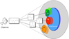Fig. 3. Sketch showing an observation of a source consisting of a linear superposition of multiple components. In this scenario, the overall profile shown on the left will be the combination of a line in emission (3e), another in absorption against the background source (2a), and a third (1) partially overlapping the background source and therefore observed in both emission (1e) and absorption (1a). See text in Sect. 3.3.2 for details.

Absorption or emission profiles. By default, SLIM considers that molecular components do not have a background continuum source other than the CMB. This is the case of component 3e in Fig. 3, where line temperature $T_{\mathrm{L}}^{3\mathrm{e}}$ will appear in emission as long as J_ν(T_ex) > J_ν(T_bg), and will rarely be observed in absorption otherwise (see Sect. 4.2).

For each component, SLIM provides the option of considering the radiative transfer effect of a background source, and therefore on the observed line temperatures. That is the case of cloud 2a in Fig. 3. The properties of the background continuum source are defined as discussed in Sect. 3.2.3. In this case the line will be observed in absorption if J_ν(T_ex) < (J_ν(T_c)+J_ν(T_bg)). In the case of cloud 2a the cloud only covers a small fraction of the continuum with a covering factor ${\theta }_{\mathrm{s}}^{2\mathrm{a}}/{\theta }_{\mathrm{c}}<1$ in Eq. (6). Although each molecule or component can have different different physical parameters and source sizes, the same continuum background spectrum is shared for all components. However, continuum effect is only applied to those molecules or components selected by the user.

Absorption and emission profiles from a single cloud. The SLIM software can also simulate the line profiles and derive the physical properties of clouds which are only partially covering the background continuum source, such as the case of component 1 in Fig. 3. In this case, two SLIM components will be added linearly with their own physical parameters. The solid angles of the two components will be such that ${\theta }_1^2={\theta }_{\text{1e}}^2-{\theta }_{\text{1a}}^2$. While 1a will consider the radiative transfer effects of a partially covered continuum emission, 1e will not include such an effect.

Kinematics – Velocity structure within the cloud. The SLIM software allows the velocity structure of the region of interest to be simulated by adding multiple velocity components for a given species such as the case of cloud 1 in Fig. 3.

Non isothermal clouds – Multiple excitation temperatures. So far, we have considered only clouds with uniform excitation temperature, a single T_ex. As a general case, molecular clouds may show internal thermal structure that can be simulated by the addition of multiple components with different excitation temperatures. The SLIM software can also handle multiple T_ex clouds by creating multiple molecular components with different T_ex. The SLIM parameters for every component can be selected independently.

However, detecting different temperature components from the observed data is sometime difficult since they usually have similar radial velocities and line widths. Moreover, if the number of transitions available is limited, it may not be straightforward to differentiate between multiple temperature components and the effects of opacity or non-LTE conditions (see Sect. 4.1 and Goldsmith & Langer 1999). To aid the user in the identification of multiple excitation temperature components, SLIM provides the functionality to generate and plot rotational diagrams (Sect. 4.1) using the observed line intensities. The resulting plots, similar to that shown in Fig. 4, can guide the initial estimates of components and temperatures. The user can derive the initial T_ex and molecular column densities by fitting straight line(s) to the rotational diagram and use them as the initial parameters for the simulation and/or the fitting of the observed line profiles.

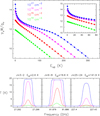Fig. 4. Upper panel: rotational diagram of the first 36 rotational transitions of HC3N generated from the SLIM output synthetic spectra. Physical parameters of Tex = 22 K, Δ = 10 km s−1 and extended source size have been used. The inset figure in the top left corner matches the range of energies displayed in Fig. 2 of Goldsmith & Langer (1999). Lower panel: synthetic spectra of three transitions at representative upper-level energies for the four column densities used to generate the rotational diagram. The effect of opacity is clearly seen in both line saturation and broadening.

The resulting observed line profile (left box in Fig. 3) will be, according to Eq. (23), the linear superposition of components and molecules. Apart from simulating and fitting observed spectra, the user can also generate and save synthetic spectra for any molecule(s) in the catalogues (Sect. 3.1) for a selected frequency range and spectral resolution, where Gaussian noise can also be added to the simulated spectra. It is important to note a few details regarding the simulation of spectra.

The sum of optical depths is only considered per component, so the optical depth of the transitions of a given molecular component are added. This is not the case for the linear superposition of components or molecules, where the sum is done in temperature or flux density units, and thus it is assumed that the different components or species are not radiatively coupled. While this assumption may be valid for velocity components, which might be actually separated within the resolution element of our observations, it may not be appropriate for multiple temperature components in the line of sight depending on the radial velocity differences and the line widths of the different components.

When modelling transitions from different observations and observatories, the beam sizes will be different. When generating the synthetic spectrum, the beam size of each of the spectra is taken into account to return the appropriate line intensities (Sect. 3.2.2).

3.4. Fitting algorithm: AUTOFIT

The AUTOFIT function of SLIM performs a non-linear least-squares fitting of simulated spectra to the data to find the optimal free parameters (N, T_ex, v_lsr, Δv and θ_s) used to generate the synthetic LTE spectra. It uses the Levenberg–Marquardt (L–M) algorithm (Levenberg 1944; Marquardt 1963) as implemented in the Herschel Common Software System²⁶ (see Press et al. 2007). The L–M algorithm combines the gradient descent method and the Gauss–Newton method to minimise the χ² function:

$$\begin{array}{c}\hfill {\chi }^2={\displaystyle \sum _i}{\left(\frac{T_i^{\mathrm{LTE}}-T_i^{\mathrm{data}}}{{\sigma }_i^2}\right)}^2,\end{array}$$(24)

where $T_i^{\text{LTE}}$ and $T_i^{\text{data}}$ are the intensities of the LTE simulation and the observed data at the spectral channel i, respectively, and σ_i is the rms noise of the data when available. When the noise is not available the weight 1/σ² is set to unity. The sum is over the relevant data channels as defined in the previous section for every transition. The SLIM implementation of the L–M algorithm does not include a priori limits set on the parameters, but they are checked during the iterative fitting procedure. Thus, the fitting procedure performs an initial check for degeneracies in the input parameters (e.g. guesses of the excitation temperature that are too large compared to the energy levels of the observed transitions, free source sizes when the result is degenerated because all transitions have been observed with the same telescope/beam, and so on). Additionally, every ten iterations of the L–M algorithm, the validity of the fitted parameters is also checked (e.g. negative excitation and molecular column densities, overly large excitation temperature compared with those of the observed transition energy levels or overly small fitted source sizes compared with the beam). In case of failing the validation, the fitting procedure stops and requests action from the user to help the convergence of the fit by changing the input parameters.

In addition to the fitted value, AUTOFIT also provides their associated error and a measure of the goodness of the fit. The errors in the fitted parameters are the 1σ standard deviations derived as follows:

$$\begin{array}{c}\hfill {\sigma }_{p_i}=\sqrt{{\mathbf{H}}^{-\mathbf{1}}(\mathbf{i},\mathbf{i})\frac{{\chi }^2}{(N-K)}},\end{array}$$(25)

with i = 1…K, which is the number of fitted parameters, N is the number of spectral data channels used in the fit, and H is the Hessian matrix derived from the inner product of the transpose of the Design matrix D(i, j) by itself.

$$\begin{array}{c}\hfill \mathbf{H}={\mathbf{D}}^T\times \mathbf{D}.\end{array}$$(26)

The Design matrix is built from the partial derivatives of the LTE line profile model for each of its parameters at the velocity of every spectral channel:

$$\begin{array}{c}\hfill \mathbf{D}(i,j)={\left(\frac{\partial T^{\mathrm{LTE}}}{\partial q_j}\right)}_i,\end{array}$$(27)

where i refers to the channel i and j to the parameter to be fitted. For completeness, in Appendix C we present the analytic derivative equations used to generate the Design matrix. The estimated errors in the fitted parameters take into the account all the data channels used in the fit, and therefore they decrease when the number of the relevant data channels, N, increases by a factor of approximately $\sqrt{N}$.

In addition to the error of the parameters, SLIM also provides information on the goodness-of-fit through the reduced or normalized $\overline{\chi }$ defined as:

$$\begin{array}{c}\hfill \overline{\chi }=\sqrt{\frac{{\chi }^2}{(N-K)}};\end{array}$$(28)

here $\overline{\chi }$ does not depend on the number of data channels used in the fit as do the errors of the parameters. The value of $\overline{\chi }$ will be different depending on the weighting of the data used in the fit. In the case that the 1/σ² weight is used, $\overline{\chi }$ should be close to 1, which is the same order of the rms noise of the data, indicating a good-quality fit. Large values of $\overline{\chi }\gg 1$, indicate a poor fit and small values of $\overline{\chi }<1$ suggest overfitting, that is the model is likely fitting some of the data noise. If the rms noise of the data is not provided to AUTOFIT, that is weight = 1 for all data points, the $\overline{\chi }$ has to be derived as the ratio between the $\overline{\chi }$ provided by AUTOFIT and the estimated rms noise of the data. Caution should be taken with the estimated $\overline{\chi }$ when the number of data channels is only slightly larger than the number of fitted parameters, since it depends of N − K. In this case the $\overline{\chi }$ might be meaningless.

Since AUTOFIT uses spectroscopically resolved line profiles, this function cannot be applied for data that do not resolve the line profiles. Upper limits to the molecular column densities can also be calculated automatically when the lines are not detected. The SLIM software estimates the local rms noise of a spectroscopic channel, σ, from the data by fitting a baseline to a selected region of the spectrum displayed in the plot that is free from line emission. The upper limit to the column density is then calculated from the upper limit to the integrated intensity

$$\begin{array}{c}\hfill {\displaystyle \int T_{\mathrm{R}}}\mathrm{\Delta }v>3\sigma \sqrt{\frac{\mathrm{\Delta }v}{\delta v}},\end{array}$$(29)

where Δv and δv are the SLIM line-width parameter and the spectral resolution of the data, respectively. The upper limit of the integrated intensity is converted to the upper limit to the column densities using the SLIM parameters, T_ex and θ_s.

4. Discussion: Limitations and degeneracies of usual molecular line radiative transfer approximations in the literature

For the sake of simplicity, a number of assumptions and/or approximations are commonly used in the literature to derive physical parameters from observed spectra (see Mangum & Shirley 2015). These latter authors explore the optically thin, thick, and R–J regimes. However, with tools like MADCUBA-SLIM, it becomes unnecessary to rely on such approximations. Rather than exploring the radiative transfer expression for different limiting cases as done by Mangum & Shirley (2015), in this section we explore the most usual approximations used in the literature for the determination of column density. Here we include the use of rotational diagrams, the analysis of absorption lines assuming a strong background continuum source, and the opacity or column density calculation from hyperfine splitting of line intensity ratios. With SLIM, not only is the use of such approximations not required, but there is also the possibility to explore the uncertainties and the range of validity of those approximations. The figures in this section, generated from the output models of SLIM, aim to explore the errors resulting from the use of approximations in the ranges where they break.

4.1. Rotational diagrams

Rotational diagrams are one of the most commonly used approximations for deriving column densities and excitation temperatures. The basics of these approximation are described in numerous references (i.e. Goldsmith & Langer 1999; Martín et al. 2006). For this approximation the basic assumptions are: no CMB: T_bg = 0; no background continuum source: T_c = 0; optically thin emission: τ_ν ≪ 1.

Therefore Eq. (6) can be combined with Eqs. (17) and (18), and in logarithmic terms we obtain the linear expression

$$\begin{array}{c}\hfill log\left(\frac{8\pi k{\nu }^2}{h{c}^3{g}_{\mathrm{u}}}{\displaystyle \int T_{\mathrm{L}}}\delta v\right)=log\left(\frac{N}{Q(T_{\mathrm{ex}})}\right)-\frac{E_{\mathrm{u}}}{k{T}_{\mathrm{ex}}}log(e).\end{array}$$(30)

The first two assumptions will hold as long as J(T_ex)≫J(T_c)+J(T_bg) which will be generally true for sources with no background continuum source. However, for low excitation, T_ex ∼ T_bg, the effect of the CMB background will not be negligible. This may be even more relevant for high-redshift studies where the the CMB temperature scales with redshift as T_bg = 2.73 (1 + z). At z = 7 the cosmic microwave background temperature is ∼22 K, and will therefore play an important role in the excitation of the molecular clouds.

Leaving aside the considerations on background temperature, the rotational diagram approximation will break for moderate to high column densities where significant deviations from linearity will occur due to the effects of increasing optical depth, which will be transition dependent. This is illustrated in Fig. 4 where the HC₃N rotational diagram has been generated out of the integrated intensities simulated by SLIM for molecular column densities ranging from 10¹⁴ to 10¹⁷ cm⁻². We simulated the emission of HC₃N assuming T_ex = 22 K and Δv = 10 km s⁻¹. The species and the physical parameters were selected to match the diagram shown in Fig. 2 of Goldsmith & Langer (1999). The inset diagram in the top left corner of Fig. 4 indeed matches the Fig. 2 of Goldsmith & Langer (1999), with the main differences being that the y-axis of their Fig. 2 is in natural logarithm scale and that the two figures show slightly different column densities. The line profiles for three out of the 36 rotational transitions used in the diagram are shown for a wide range of upper energy levels, where the effect of line saturation and line broadening (Eq. (21)) are evidenced even for high-energy transitions.

The curvature of the rotational diagram (blue and magenta points in Fig. 4), together with an insufficient sampling in the number of observed transitions, can lead to the misidentification of multiple temperature components. This section shows that SLIM correctly takes into account the effects of increasing optical depth in the molecular transitions. In any case, as mentioned in Sect. 3.3.2 when referring to non-isothermal modelling, the use of rotational diagrams may help as a first guide for initial fitting parameters in models with multiple temperatures.

It is important to mention here the limitation regarding the LTE assumption. Figure 6 in Goldsmith & Langer (1999) shows how non-LTE effects do also break the linearity when the emission is not thermalised. Thus, if molecular hydrogen volume density is below the critical density (n(H₂) < n_crit) of any given transition, the LTE assumption in SLIM will also break. As a result, curved rotational diagrams would reveal a degeneracy between low-density subthermal excitation or multiple high-density components such as those observed in the CO ladder towards Sgr A^* (Goicoechea et al. 2013).

4.2. Absorption profiles

Most studies of absorption molecular profiles display the normalized spectra in order to directly measure the fraction of the continuum absorbed by foreground gas. Thus, instead of defining the line temperature after subtracting the continuum in Eq. (6), the fraction of absorption of the continuum can be written as

$$\begin{array}{c}\hfill \frac{T_{\mathrm{L}}}{J(T_{\mathrm{c}})}=\frac{(J_{\nu }(T_{\mathrm{ex}})-c_{\mathrm{s}}{J}_{\nu }(T_{\mathrm{c}})-J_{\nu }(T_{\mathrm{bg}}))(1-{\mathrm{e}}^{-{\tau }_{\nu }})}{J(T_{\mathrm{c}})}·\end{array}$$(31)

If we assume that the absorption is occurring against a very bright continuum source, which implies that T_c ≫ T_bg and T_c ≫ T_ex. Then Eq. (31) reduces to

$$\begin{array}{c}\hfill {\tau }_{\nu }=-ln(1-\frac{T_{\mathrm{L}}}{c_{\mathrm{s}}J(T_{\mathrm{c}})}),\end{array}$$(32)

which is commonly used to quickly estimate the opacity of the absorption profiles towards bright continuum emitters (i.e. Muller et al. 2011). This expression, where c_s is usually considered to be unity, is independent of the excitation temperature of the gas. Figure 5 shows the optical depth of the CO J = 1−0 profile calculated by MADCUBA for fixed values of Δv = 10 km s⁻¹, log N = 17 cm⁻², and T_bg = 2.73 K as a function of varying T_ex. Figure 5 also displays the optical depth calculated based on the generated synthetic spectra and with the approximation in Eq. (32). These optical depths are calculated as a function of the assumed T_ex and for two background continuum black bodies with temperatures T_c of 10 and 100 K (top and bottom panels in Fig. 5, respectively).

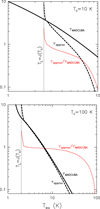Fig. 5. Optical depth of the absorption profile of CO 1-0 calculated by MADCUBA (black continuous line) for Δv = 10 km s−1, log N = 17 cm−2, and Tbg = 2.73 K. From the values measured in the synthetic spectra and using Eq. (32), the approximate optical depth is calculated (black dashed line). The ratio between the two optical depth estimates is shown in red. Top and bottom panels are equal but for the continuum temperatures of 10 and 100 K, respectively. Vertical dotted line represent the temperature for which the line completely absorbs the continuum emission (i.e. TL = J(Tc)), and beyond which the CMB continuum is absorbed.

Figure 5 shows that the optical depth is actually temperature dependant. However, it also illustrates, as explained below, the range in which this approximation to estimate the optical depth is valid, which is relative to the brightness of the illuminating continuum source. The ratio between both optical depths is also displayed as a red line to better show the region where the approximation holds.

Figure 5 shows that when T_ex approaches the CMB temperature (in this case T_bg = 2.73 K), the approximation in Eq. (32) goes to infinity since the continuum is completely absorbed (T_L = J(T_c), dotted vertical line in Fig. 5). Albeit unusual, the approximation in Eq. (32) will not apply for temperatures below the CMB temperature (T_ex <  T_bg), where the normalized absorption is negative since it absorbs the CMB continuum (see Martin-Pintado et al. 1985, and references therein). Similarly, high optical depths can be the result of very high column densities. In this situation, the fit to the line profile by MADCUBA, and in particular line-profile broadening (Eq. (21)), will allow for a more accurate estimate of the optical depth than simply basing estimations on the intensity of the absorption.

For excitation temperatures approaching that of the background continuum (T_ex  ∼  T_c), the absorption will vanish and therefore the opacity calculated based on the approximation in Eq. (32) will be severely underestimated. This is particularly critical for faint background illuminating continuum sources (i.e. search for absorption against faint GRB events; de Ugarte Postigo et al. 2018) where a non-detection of absorption may be either low absorbing column density or significant amounts of gas not seen in absorption due to T_ex ∼ T_c.

For temperatures in between the CMB temperature and the temperature of the background continuum source, the optical depth estimated with Eq. (32) has a relatively narrow range of validity outside of which the approximation, and therefore the derived column density, will be over or underestimated for low or high excitation temperatures, respectively.

With SLIM, the user does not need to make the assumptions mentioned above, and through educated guesses of the excitation temperature it will be possible for the user to estimate the errors in the optical depths and column densities derived from the observations. Moreover, the SLIM simulation will also help the user to prepare the observations that will provide the best estimate of the excitation temperature by measuring several transitions.

4.3. Molecular line opacities from hyperfine splitting

As commonly used in the literature (i.e. Henkel et al. 1998), the ratio of the line intensities of two molecular transitions (or blended groups of transitions) can be written as

$$\begin{array}{c}\hfill \frac{T_{\mathrm{L},1}}{T_{\mathrm{L},2}}=\frac{1-{\mathrm{e}}^{-{\tau }_1}}{1-{\mathrm{e}}^{-{\tau }_2}},\end{array}$$(33)

where this expression implicitly assumes no background continuum source: T_c = 0 and LTE conditions (T_ex, 1 = T_ex, 2).

Hyperfine transition splitting in molecules provides a way of directly inferring the optical depth of the emission through the observed hyperfine line intensity ratios. In the optically thin regime, the ratio between any given pair of hyperfine lines is directly related to the ratio between their optical depths τ₁/τ₂, under the above-mentioned assumptions. Since most spectroscopic parameters (frequencies, energy levels, and Einstein coefficients) are almost identical, from Eq. (19) this optical depth ratio will be equal to the ratio between involved hyperfine transition upper level degeneracies τ₁/τ₂ = g_u, 1/g_u, 2.

As a case study we consider here the J = 1−0 transition of N₂H⁺ which is split into three hyperfine components F = 2−1, 1−1, and 0−1 at 93173.7, 93171.88, and 93176.13 MHz, respectively (based on the spectroscopy from the JPL catalogue). In Fig. 6 we show the opacity of the brightest component τ₂₁ as a function of the ratio of the F = 2−1 to the F = 0−1 transition. In the optically thin regime, as explained above, the ratio between the line intensities will approach that of the ratio of the upper-level degeneracies (g₂₁ = 15 and g₀₁ = 3), and therefore τ₂₁/τ₀₁ = 5. On the other hand, as the optical depth grows towards the optically thick regime, both spectral lines will saturate and their ratio will asymptotically approach unity (see Eq. (33)).

Fig. 6. Optical depth to the F = 2−1 hyperfine transition of N2H+ as a function of the ratio of the line intensities of the F = 2−1 to the F = 0−1 shown in black. The line width used in the SLIM simulations is Δv = 2 km s−1 to avoid blending between hyperfine transitions. In red and blue we represent the propagated uncertainties considering that the F = 2−1 hyperfine transitions of N2H+ are detected with S/Ns of 50 and 20, respectively. See Sect. 4.3 for details.

Despite the relation between line intensities and optical depths, albeit the approximations above, the intrinsic uncertainties to the line temperature measurements may translate into large uncertainties in the estimated optical depth as we get close to the limiting cases. In Fig. 6, we show the actual relation with a thick black line, while the red and blue lines show the uncertainty in the derived optical depth by assuming a signal-to-noise ratio (S/N) in the F = 2−1 transition (S/N = T₂₁/rms, where rms is the noise of the spectra) of 50 and 20, respectively. The uncertainty in the optical depth is calculated via the error propagation (using its numerical derivative) as $\mathrm{\Delta }{\tau }_{21}=\left(\frac{\partial {\tau }_{21}}{\partial r}\right)\mathrm{\Delta }r$, where the uncertainty on the line ratio (r) is calculated as $\mathrm{\Delta }r=r\sqrt{1+r^2}/S/N$. In the optically thin regime, as we approach the theoretical value of 5, the uncertainties in the optical depth, and therefore in the column density determination, may vary by several orders of magnitude. Furthermore, towards the optically thick regime, though not as severe, the optical depth can be easily uncertain by a factor of a few. It is only within the range of τ₂₁ between ∼1−10, that the optical depth would be well constrained.

We note that the large uncertainties in the optically thin regime is a result of the decreased S/N of the F = 0−1 line, which being a factor of five fainter than the F = 2−1, would be detected at S/Ns of 10 and 4, for the two examples shown in Fig. 6. The same study could be carried out with the ratio of the F = 2−1 to 1−1, since the latter is brighter than the 0−1 by τ₂₁/τ₁₁ = g₂₁/g₁₁ ∼ 1.66. However, in this case, the dynamic range of the ratio will be limited to the range from 1.66 in the optically thin regime to 1 in the thick end.

Once the opacity is estimated from the line intensity ratio, column density can be derived via an assumption on the excitation temperature as represented with the black dashed lines in Fig. 7. In this latter figure, we added the predicted line intensity in main beam brightness temperature scale as it would be observed with the 26.4″ beam of the IRAM 30 m telescope at the frequency of this transition. Each colour represents an iso-line-temperature contour for an extended source (continuous line), and a source size of two thirds and one third of the telescope beam (dashed and dotted line, respectively). This figure includes the effect of the CMB, but no other background continuum source.

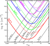Fig. 7. Column density of N2H+ as a function of the estimated optical depth (Fig. 6) of its J = 1−0, F = 2−1 transition for different assumed excitation temperatures (black dashed lines). In colour we represent isotemperature curves of simulated line intensities in main beam temperature scale for the 26.4″ primary beam of the IRAM 30 m at the frequency of this transition. The curves are calculated for different source sizes: extended (continous line); two thirds of the primary beam (dashed); and one third of the primary beam (dotted). The simulation considers a line width Δv = 2 km s−1, and Tbg = 2.73 K.

The main idea behind Fig. 7 is to illustrate the fact that apart from the line intensity ratio used to derive the optical depth of the emission, the absolute measured line intensity provides valuable information that may allow to break the degeneracy between optical depth, excitation temperature, and source size (see Eq. (9)). In other words, once the opacity has been measured with the hyperfine structure, it is not possible to determine the column density with prior assumptions on the excitation temperature and source size, since this may not fit the actual line intensity measured. Since SLIM fits directly the observed spectrum by varying the physical parameters, both the absolute line intensity and intensity ratio are fitted simultaneously.

Therefore, if we have good a priori information on the excitation temperature, the line intensity may provide constraints on the source size. On the other hand the line intensity can also set constraints on the possible excitation temperatures with a priori information on the source size. This allows for determination of excitation temperatures based on a single hyperfine split transition if not in the optically thin or thick regime. Figure 7 is valid for this particular transition of N₂H⁺, but similar plots could be generated for other transitions or molecules. Additionally, when a particular transition becomes optically thick, the line broadening by opacity (Eq. (21)) can be used to further break the degeneracy between physical parameters.

The above discussion also applies to non-hyperfine split transitions. In this latter case, opacity will not be constrained by the line intensity ratio and the degeneracy will be directly on column density, excitation temperature, and source size. Any combination of these parameters will have to reproduce the observed line intensity.

Figure 7 shows how by fitting the line profile as a whole with SLIM we can constrain the physical parameters of column density and excitation temperature. More importantly, SLIM allows the user to easily explore the parameter space and observe the effect of the changes in the line profile on-the-fly by varying input parameters.

5. Conclusion

In this paper we present the main functionalities of the highly interactive spectroscopic data handling package MADCUBA and its spectroscopy analysis module SLIM. The basic radiative transfer formalism and fitting algorithm used by SLIM have been described in detail. We discuss the usual approximations used in the literature for different limit cases that simplify the radiative transfer equation in order to derive physical parameters. We show that these approximations may result in both significant deviations in the derived parameters, when the assumptions for such approximations break, as well as in underestimation of the errors associated to those approximations. More importantly, we show that with modern tools like MADCUBA and SLIM, there is no need to resort to those approximations since we can easily model the observed spectra using the full radiative transfer equation. We also note that, by design, SLIM works under the LTE assumption, and therefore does not apply to non-LTE conditions or under non-LTE excitation.

MADCUBA and SLIM, as with other tools open to the community, allow for efficient handling of large spectroscopic datasets that are due to come from state-of-the-art radio, millimetre, and sub-millimetre facilities.

Acknowledgments

The MADCUBA and SLIM development has been partially funded through the Spanish grants ESP2013-21697-C05-01, ESP2015-65597-C4-01-R and ESP2017-86582-C4-01-R. V. M. R. has received funding from the European Union’s Horizon 2020 research and innovation programme under the Marie Skłodowska-Curie grant agreement No. 664931. S. M. and V. M. R. acknowledge support from the Joint ALMA Observatory Visitor Program.

References

Appendix A: Units included in MADCUBA

In this section we present a comprehensive list of the units managed by MADCUBA.

A.1. Spectral units

We refer the reader to Greisen et al. (2006) for a complete description of the spectral coordinates representation and conversion between the units below.

• Frequency (rest and observed): Hz, KHz, MHz, GHz, THz

• Wavenumbers: cm⁻¹, m⁻¹

• Energy: eV, J, ergs

• Wavelength (rest and observed): Å, nm,μm, mm, m

• Velocity (radio, optical, and relativistic): ms⁻¹, kms⁻¹

• Redshift: z

• Beta factor: β = v/c

A.2. Intensity units

• –

  [μ | m] K

• –

  [μ | m] Jy beam⁻¹

• –

  [μ | m] Jy arcsec⁻²

• –

  [μ | m|M] Jy sr⁻¹

• –

  [μ | m] K spaxel⁻¹

• –

  W [cm | m]⁻²Hz⁻¹sr⁻¹

• –

  W [cm | m]⁻² [Å | nm |μm]⁻¹sr⁻¹

• –

  ergss⁻¹cm⁻²Hz⁻¹sr⁻¹

• –

  ergss⁻¹cm⁻² [Å | nm |μm]⁻¹sr⁻¹

A.3. Flux density units

• [μ | m | M] Jy

• W [cm | m]⁻²Hz⁻¹

• W [cm | m]⁻² [Å | nm |μm]⁻¹

• ergss⁻¹ [cm | m]⁻²Hz⁻¹

• ergss⁻¹ [cm | m]⁻² [Å | nm |μm]⁻¹

A.4. Integrated flux density units

• [μ | m | M] Jy Hz

• W [cm | m]⁻²

• ergss⁻¹cm⁻²

A.5. Integrated Intensity units

• K Hz

• [μ | m] K [km | m] s⁻¹

• [μ | m] Jy beam⁻¹ [km | m] s⁻¹

• [μ | m] Jy arcsec⁻² [km | m] s⁻¹

• [μ | m | M] Jy sr⁻¹ [km | m] s⁻¹

• [μ | m] Jy spaxel⁻¹ [km | m] s⁻¹

• W [cm | m]⁻²sr⁻¹

• ergs⁻¹cm⁻²sr⁻¹

Appendix B: MADCUBA sample files

Although we refer to the documentation which is developing in the MADCUBA webpage²⁷, in this appendix we include a sample of input files to illustrate the format required by MADCUBA and SLIM.

B.1. Input spectra in ASCII format

In order to import spectra from any data source, it is possible to use a simple ASCII file where the key spectral parameters can be provided as the following sample file.

Unit Angle : deg
Unit Spectral : Hz
Unit Velo : km/ s
Unit Inten : K
TempScale : TA∗
Beammaj : 0.002777778
Beammin : 0.001388889
BeamPA: 20
CoordType= EQU
CoordProj :GLS
Epoch= 2000
sRadesys=FK5"
XCoord= 66.666
yCoord= −10.1010
VeloType : VRAD−LSR
Velocity= 40
xLabel :FREQ−LSR
Rest Freq : 8 . 8E+10
ylabel : Intensity
// Data x_values1 , y_values1 , error 1
 8.7992763427734E+10 −0.014919484034181
 8.7994763427734E+10 −0.016418563202024
 8.7996763427734E+10 −0.011609123088419
 8.7998763427734E+10 −4.1951001621783E−03
 8.8000763427734E+10 −1.797300792532E−04
 8.8002763427734E+10 −6.2841214239597E−03

We note the importance of the unit definition at the top of the file, which will determine the input unit of the different parameters. However, it is not necessary to provide values for all parameters. The sample below defines the basic header that includes the spectral units and intensity units, and within a single file inputs fours spectra that MADCUBA will load as individual spectra:

# mycube_band4_spw1.image−raster
UnitSpectral: GHz
UnitInten: Jy/beam

9.983684539795e+01 2.884732144998e−03
9.980559539795e+01 2.525573612008e−03
9.977434539795e+01 2.476226447418e−03

# mycube_band4_spw2.image−raster
UnitSpectral: GHz
UnitInten: Jy/beam
1.074863204956e+02 3.165612609541e−03
1.075175704956e+02 3.662855322292e−03
1.075488204956e+02 3.426149531019e−03

# mycube_band6_spw1.image−raster
UnitSpectral: GHz
UnitInten: Jy/beam
1.056113967896e+02 3.483511136527e−03
1.056426467896e+02 2.839534894392e−03
1.056738967896e+02 3.722954211636e−03

# mycube_band6_spw2.image−raster
UnitSpectral: GHz
UnitInten: Jy/beam
9.733055114746e+01 2.297109951407e−03
9.729930114746e+01 3.345324198354e−03
9.726805114746e+01 1.939967128391e−03

We note that the lines defining the unit will be used to demarcate individual concatenated spectra within a single input file. For each spectrum in the file, any non-defined parameter will be set to the default units.

B.2. Sample MADCUBA script

The best way to create scripts (macros) in ImageJ and therefore in MADCUBA is through the macro recorder that can be accessed through the Macros menu in MADCUBA or directly through Plugins>Macros>Record within the ImageJ interface. The file below, created through the macro recorder, shws a sample script that imports three ALMA data cubes, closes them, opens the imported MADCUBA created fits cubes, extracts the spectrum from the two regions of interest (in this case, a pixel and a rectangle defined in the reference cube) and writes it to an output spectra file.

// Import the casa cubes into MADCUBA fits files , changing the velocity
run ("Import ALMA CUBE FITS FILE" , "select=‘/path/spw1.cube.fits’
change head=’Vrad$180$km/s#’");
select Window ("PLOT MAD_CUB_spw1.cube.fits");
close ( );
select Window ("CUBE MAD_CUB_spw1.cube.fits");
close ( );
run ("Import ALMA CUBE FITS FILE",
"select =’/path/spw2.cube.fits’change head=’Vrad$180$km/s#’");
select Window ("PLOT MAD_CUB_spw1.cube.fits");
close ( );
select Window ("CUBE MAD_CUB_spw1.cube.fits");
close ( );
run ("Import ALMA CUBE FITS FILE", "select =’/path/spw3.cube.fits’
change head=’Vrad$180$km/s#’");
select Window ("PLOT MAD_CUB_spw1.cube.fits");
close ( );
select Window ("CUBE MAD_CUB_spw1.cube.fits");
close ( );
// Open the Master cube, which will be the reference for all the others.
run ("Open Virtual Cube",
"writemacro=true select =’/mypath/MAD_CUB_spw1.cube.fits’");
// Open all other cubes
run ("Open Virtual Cube Background", "select =’/mypath/MAD_CUB_spw2.cube.fits’");
run ("Open Virtual Cube Background", "select =’/mypath/MAD_CUB_spw3.cube.fits’");
run ("Synchronize Cube", "");
// INFO: Synchronize List selected Cube
run ("Synchronize select Cube", "name_cube=ALL");
select Window ("CUBE MAD_CUB_spw1.cube.fits");
// select the Region of Interest (ROI)
// Extracting spectra in a single pixel
make Rectangle (69, 96, 1, 1);
run ("Synchronize Roi Cube", "cursorroi=true coords=true");
run ("Synchronize Cube", "");
run ("Extract Spectra Sync Integrated", "select =’/mypath/singlepixelROI.fits’");
// EXTRACTING POSITION 2
make Rectangle (69, 96, 10, 10);
run ("Synchronize Roi Cube", "cursorroi=true coords=true");
run ("Synchronize Cube", "");
run ( " Extract Spectra Sync Integrated", "select=’/mypath/rectangleROI.fits’");
close( );

B.3. Continuum by user input file

The continuum of a spectrum can be added as a user input in a simple two-column file consisting of the frequency in Hertz and the intensity, in the units of the current open spectra, at that frequency. Here is a simple sample continuum input file.

604. 0E+09 ,0.0018
671. 0E+09 ,0.0027
758. 0E+09 ,0.0040
903. 0E+09 ,0.0066
995. 0E+09 ,0.0085
1025.0E+09 ,0.0096
1043.0E+09 ,0.0104

We note that continuum values will be interpolated in between the values in the file.

Appendix C: Detailed derivative equations for fitting algorithms

Here we present the analytic derivative equations of the Eq. (9) used to generate the Design matrix (Sect. 3.4).

For the sake of simplicity, we rewrite Eq. (23) to represent the intensity measured in the corresponding units for a single molecule and component as

$$\begin{array}{c}\hfill I=U_{\mathrm{f}}{J}_{\mathrm{TOT}}(1-{\mathrm{e}}^{-{\displaystyle {\sum }_t}{\tau }_{\mathrm{o}}^t\mathrm{\Phi }}),\end{array}$$(C.1)

where we have defined the Gaussian shape (Φ) and the total intensity in temperature units (J_TOT) as

$$\begin{array}{cc}& \mathrm{\Phi }={\mathrm{e}}^{-4ln2{(v-v_{°})}^2/\mathrm{\Delta }{v}^2},\hfill \end{array}$$(C.2)

$$\begin{array}{cc}& J_{\mathrm{TOT}}=(J_{\nu }(T_{\mathrm{ex}})-J_{\nu }(T_{\mathrm{bg}})-J_{\nu }(T_{\mathrm{c}})),\hfill \end{array}$$(C.3)

and the unit factor U_f will be either $\frac{{\theta }_{\mathrm{s}}^2}{{\theta }_{\mathrm{s}}^2+{\theta }_{\mathrm{b}}^2}$ (for units of main beam temperature T_MB) or ${10}^{23}\frac{2k{\nu }^2}{c^2}1.133{\theta }_{\mathrm{s}}^2$ (for units of flux density S), as introduced in Eq. (9).

$$\begin{array}{cc}& \frac{\delta I}{\delta N}=U_{\mathrm{f}}{J}_{\mathrm{TOT}}\left({\mathrm{e}}^{-{\displaystyle {\sum }_i}{\tau }_{\mathrm{o}}^i\mathrm{\Phi }}\frac{1}{N}{\displaystyle \sum _i}{\tau }_{\mathrm{o}}^i\mathrm{\Phi }\right)\hfill \end{array}$$(C.4)

$$\begin{array}{cc}& \frac{\delta I}{\delta T_{\mathrm{ex}}}=U_{\mathrm{f}}(J{(T_{\mathrm{ex}})}^2\frac{{\mathrm{e}}^{h\nu /k{T}_{\mathrm{ex}}}}{T_{\mathrm{ex}}^2}(1-{\mathrm{e}}^{-{\displaystyle {\sum }_i}{\tau }_{\mathrm{o}}\mathrm{\Phi }})\hfill \\ \hfill & +J_{\mathrm{TOT}}({\mathrm{e}}^{-{\displaystyle {\sum }_i}x{\tau }_{\mathrm{o}}^i\mathrm{\Phi }}{\displaystyle \sum _i}{\tau }_{\mathrm{o}}^i\hfill \\ \hfill & \times \mathrm{\Phi }(\frac{(E_{\mathrm{l}}{\mathrm{e}}^{-E_{\mathrm{l}}/k{T}_{\mathrm{ex}}}-E_{\mathrm{u}}{\mathrm{e}}^{-E_{\mathrm{u}}/k{T}_{\mathrm{ex}}})}{k{T}_{\mathrm{ex}}^2({\mathrm{e}}^{-E_{\mathrm{l}}/k{T}_{\mathrm{ex}}}-{\mathrm{e}}^{-E_{\mathrm{u}}/k{T}_{\mathrm{ex}}})}-\frac{1}{Q(T_{\mathrm{ex}})}\frac{\delta Q(T_{\mathrm{ex}})}{\delta T_{\mathrm{ex}}})))\hfill \end{array}$$(C.5)

$$\begin{array}{cc}& \frac{\delta I}{\delta v_{°}}=U_{\mathrm{f}}{J}_{\mathrm{TOT}}({\mathrm{e}}^{-{\displaystyle {\sum }_i}{\tau }_{\mathrm{o}}^i\mathrm{\Phi }}{\displaystyle \sum _i}(\frac{8ln2(v-v_{°})}{\mathrm{\Delta }{v}^2}{\tau }_{\mathrm{o}}^i\mathrm{\Phi }))\hfill \end{array}$$(C.6)

$$\begin{array}{cc}& \frac{\delta I}{\delta \mathrm{\Delta }v}=U_{\mathrm{f}}{J}_{\mathrm{TOT}}({\mathrm{e}}^{-{\displaystyle {\sum }_i}{\tau }_{\mathrm{o}}^i\mathrm{\Phi }}{\displaystyle \sum _i}\frac{{\tau }_{\mathrm{o}}^i\mathrm{\Phi }}{\mathrm{\Delta }v}(\frac{8ln2{(v-v_{°})}^2}{\mathrm{\Delta }{v}^2}-1))\hfill \end{array}$$(C.7)

$$\begin{array}{cc}& \frac{\delta I}{\delta \mathrm{\Delta }{\theta }_{\mathrm{s}}}=U{\prime }_{\mathrm{f}}{J}_{\mathrm{TOT}}(1-{\mathrm{e}}^{-{\displaystyle {\sum }_t}{\tau }_{\mathrm{o}}^t\mathrm{\Phi }})\hfill \end{array}$$(C.8)

where $U{\prime }_{\mathrm{f}}=\frac{\delta U_{\mathrm{f}}}{{\theta }_{\mathrm{s}}}$ will be $\frac{2}{{\theta }_{\mathrm{s}}}(\frac{{\theta }_{\mathrm{s}}^2}{({\theta }_{\mathrm{s}}^2+{\theta }_b^2)}-(\frac{{\theta }_{\mathrm{s}}^2}{({\theta }_{\mathrm{s}}^2+{\theta }_b^2)}{)}^2)$ in T_MB units, and ${10}^{23}2.266{\theta }_{\mathrm{s}}\frac{2k{\nu }^2}{c^2}$ in S units.

In order to derive the partial derivatives of the measured intensity above, the partial derivatives of the central optical depth, Gaussian shape, and total intensity are required. For completeness, we write the expression of these derivatives below. We note that the partial derivative of the partition function with respect to the excitation temperature ($\frac{\delta Q(T_{\mathrm{ex}})}{\delta T_{\mathrm{ex}}}$) appearing in $\frac{\delta I}{\delta T_{\mathrm{ex}}}$ is approximated in SLIM by the linear slope of the the partition function between the two values from the catalogue entries surrounding a given excitation temperature.

$$\begin{array}{cc}& \frac{\delta U_{\mathrm{f}}{J}_{\mathrm{TOT}}}{\delta N}=0\hfill \end{array}$$(C.9)

$$\begin{array}{cc}& \frac{\delta U_{\mathrm{f}}{J}_{\mathrm{TOT}}}{\delta T_{\mathrm{ex}}}=U_{\mathrm{f}}J{(T_{\mathrm{ex}})}^2\frac{{\mathrm{e}}^{h\nu /k{T}_{\mathrm{ex}}}}{T_{\mathrm{ex}}^2}\hfill \end{array}$$(C.10)

$$\begin{array}{cc}& \frac{\delta U_{\mathrm{f}}{J}_{\mathrm{TOT}}}{\delta v_{°}}=0\hfill \end{array}$$(C.11)

$$\begin{array}{cc}& \frac{\delta U_{\mathrm{f}}{J}_{\mathrm{TOT}}}{\delta \mathrm{\Delta }v}=0\hfill \end{array}$$(C.12)

$$\begin{array}{cc}& \frac{\delta U_{\mathrm{f}}{J}_{\mathrm{TOT}}}{\delta {\theta }_{\mathrm{s}}}=U{\prime }_{\mathrm{f}}{J}_{\mathrm{TOT}}\hfill \end{array}$$(C.13)

$$\begin{array}{cc}& \frac{\delta {\tau }_{\mathrm{o}}}{\delta N}=\frac{{\tau }_{\mathrm{o}}}{N}\hfill \end{array}$$(C.14)

$$\begin{array}{cc}& \frac{\delta {\tau }_{\mathrm{o}}}{\delta T_{\mathrm{ex}}}={\tau }_{\mathrm{o}}(\frac{(E_{\mathrm{l}}{\mathrm{e}}^{-E_{\mathrm{l}}/k{T}_{\mathrm{ex}}}-E_{\mathrm{u}}{\mathrm{e}}^{-E_{\mathrm{u}}/k{T}_{\mathrm{ex}}})}{k{T}_{\mathrm{ex}}^2({\mathrm{e}}^{-E_{\mathrm{l}}/k{T}_{\mathrm{ex}}}-{\mathrm{e}}^{-E_{\mathrm{u}}/k{T}_{\mathrm{ex}}})}-\frac{1}{Q(T_{\mathrm{ex}})}\frac{\delta Q(T_{\mathrm{ex}})}{\delta T_{\mathrm{ex}}})\hfill \end{array}$$(C.15)

$$\begin{array}{cc}& \frac{\delta {\tau }_{\mathrm{o}}}{\delta v_{°}}=0\hfill \end{array}$$(C.16)

$$\begin{array}{cc}& \frac{\delta {\tau }_{\mathrm{o}}}{\delta \mathrm{\Delta }v}=-\frac{{\tau }_{\mathrm{o}}}{\mathrm{\Delta }v}\hfill \end{array}$$(C.17)

$$\begin{array}{cc}& \frac{\delta {\tau }_{\mathrm{o}}}{\delta {\theta }_{\mathrm{s}}}=0\hfill \end{array}$$(C.18)

$$\begin{array}{cc}& \frac{\delta \mathrm{\Phi }}{\delta N}=0\hfill \end{array}$$(C.19)

$$\begin{array}{cc}& \frac{\delta \mathrm{\Phi }}{\delta T_{\mathrm{ex}}}=0\hfill \end{array}$$(C.20)

$$\begin{array}{cc}& \frac{\delta \mathrm{\Phi }}{\delta v_{°}}=\frac{8ln2(v-v_{°})}{\mathrm{\Delta }{v}^2}\mathrm{\Phi }\hfill \end{array}$$(C.21)

$$\begin{array}{cc}& \frac{\delta \mathrm{\Phi }}{\delta \mathrm{\Delta }v}=\frac{8ln2{(v-v_{°})}^2}{\mathrm{\Delta }{v}^3}\mathrm{\Phi }\hfill \end{array}$$(C.22)

$$\begin{array}{cc}& \frac{\delta \mathrm{\Phi }}{\delta {\theta }_{\mathrm{s}}}=0\hfill \end{array}$$(C.23)

All Figures

Fig. 1. Screenshot showing the use of MADCUBA to spatially synchronise multiple datacubes. In this case, eight ALMA datacubes taken from the data published by Martín et al. (2019) are loaded and synchronised. From top to bottom and left to right, the windows shown are: the main ImageJ window; the main MADCUBA menu; the cube container window displaying the currently opened data cubes; the synchronise cube window listing the data cubes currently synchronised (in this case all opened ones); the cube display where the selected channel of the first opened data cube is displayed and the RoI is interactively defined (black contour on image); and finally the eight spectra corresponding to the integrated spectra from the RoI for each synchronised datacube. We note that the image channel displayed is selected with a red line in the top left spectrum, which corresponds to the spectrum from the cube displayed.

In the text

Fig. 2. Screenshot showing the use of SLIM within MADCUBA to identify and fit a synthetic LTE model to an observed broadband spectrum. In this case, a 30 000 channel ALMA spectrum is displayed where more than 100 molecular species have been fitted. From top to bottom and left to right, the windows shown are: the main ImageJ window; the main MADCUBA menu; the modelling tab within the SLIM tool with the list of fitted species and the sliders in the bottom to interactively adjust the physical parameters; the spectra container window displaying the currently opened spectra; the plot showing the full spectrum with the transitions of the selected species labeled; the SLIM PLOT showing the synthetic model overlaid on top of the observed spectra zoomed to the brightest transitions of the selected species; the list of transitions of the selected species.

In the text

Fig. 3. Sketch showing an observation of a source consisting of a linear superposition of multiple components. In this scenario, the overall profile shown on the left will be the combination of a line in emission (3e), another in absorption against the background source (2a), and a third (1) partially overlapping the background source and therefore observed in both emission (1e) and absorption (1a). See text in Sect. 3.3.2 for details.

In the text

Fig. 4. Upper panel: rotational diagram of the first 36 rotational transitions of HC3N generated from the SLIM output synthetic spectra. Physical parameters of Tex = 22 K, Δ = 10 km s−1 and extended source size have been used. The inset figure in the top left corner matches the range of energies displayed in Fig. 2 of Goldsmith & Langer (1999). Lower panel: synthetic spectra of three transitions at representative upper-level energies for the four column densities used to generate the rotational diagram. The effect of opacity is clearly seen in both line saturation and broadening.

In the text

Fig. 5. Optical depth of the absorption profile of CO 1-0 calculated by MADCUBA (black continuous line) for Δv = 10 km s−1, log N = 17 cm−2, and Tbg = 2.73 K. From the values measured in the synthetic spectra and using Eq. (32), the approximate optical depth is calculated (black dashed line). The ratio between the two optical depth estimates is shown in red. Top and bottom panels are equal but for the continuum temperatures of 10 and 100 K, respectively. Vertical dotted line represent the temperature for which the line completely absorbs the continuum emission (i.e. TL = J(Tc)), and beyond which the CMB continuum is absorbed.

In the text

Fig. 6. Optical depth to the F = 2−1 hyperfine transition of N2H+ as a function of the ratio of the line intensities of the F = 2−1 to the F = 0−1 shown in black. The line width used in the SLIM simulations is Δv = 2 km s−1 to avoid blending between hyperfine transitions. In red and blue we represent the propagated uncertainties considering that the F = 2−1 hyperfine transitions of N2H+ are detected with S/Ns of 50 and 20, respectively. See Sect. 4.3 for details.

In the text

Fig. 7. Column density of N2H+ as a function of the estimated optical depth (Fig. 6) of its J = 1−0, F = 2−1 transition for different assumed excitation temperatures (black dashed lines). In colour we represent isotemperature curves of simulated line intensities in main beam temperature scale for the 26.4″ primary beam of the IRAM 30 m at the frequency of this transition. The curves are calculated for different source sizes: extended (continous line); two thirds of the primary beam (dashed); and one third of the primary beam (dotted). The simulation considers a line width Δv = 2 km s−1, and Tbg = 2.73 K.

In the text

References

- Aladro, R., Martín, S., Riquelme, D., et al. 2015, A&A, 579, A101 [NASA ADS] [CrossRef] [EDP Sciences] [Google Scholar]
- Armijos-Abendaño, J., López, E., Martín-Pintado, J., et al. 2018, MNRAS, 476, 2446 [NASA ADS] [CrossRef] [Google Scholar]
- Baez, A. 2014, PhD Thesis, Universidad Complutense de Madrid [Google Scholar]
- Beltrán, M. T., Cesaroni, R., Rivilla, V. M., et al. 2018, A&A, 615, A141 [NASA ADS] [CrossRef] [EDP Sciences] [Google Scholar]
- Colzi, L., Fontani, F., Rivilla, V. M., et al. 2018, MNRAS, 478, 3693 [NASA ADS] [CrossRef] [Google Scholar]
- Cosentino, G., Jiménez-Serra, I., Henshaw, J. D., et al. 2018, MNRAS, 474, 3760 [NASA ADS] [Google Scholar]
- de Ugarte Postigo, A., Thöne, C. C., Bolmer, J., et al. 2018, A&A, 620, A119 [NASA ADS] [CrossRef] [EDP Sciences] [Google Scholar]
- Downes, D. 1989, in Evolution of Galaxies: Astronomical Observations, eds. I. Appenzeller, H. J. Habing, & P. Lena (Berlin: Springer Verlag), Lecture Notes in Physics, 333, 351 [NASA ADS] [CrossRef] [Google Scholar]
- Endres, C. P., Schlemmer, S., Schilke, P., Stutzki, J., & Müller, H. S. P. 2016, J. Mol. Spectrosc., 327, 95 [Google Scholar]
- Goicoechea, J. R., Etxaluze, M., Cernicharo, J., et al. 2013, ApJ, 769, L13 [NASA ADS] [CrossRef] [Google Scholar]
- Goldsmith, P. F., & Langer, W. D. 1999, ApJ, 517, 209 [NASA ADS] [CrossRef] [Google Scholar]
- Greisen, E. W., Calabretta, M. R., Valdes, F. G., & Allen, S. L. 2006, A&A, 446, 747 [NASA ADS] [CrossRef] [EDP Sciences] [Google Scholar]
- Harada, N., Sakamoto, K., Martín, S., et al. 2018, ApJ, 855, 49 [NASA ADS] [CrossRef] [Google Scholar]
- Henkel, C., Chin, Y., Mauersberger, R., & Whiteoak, J. B. 1998, A&A, 329, 443 [NASA ADS] [Google Scholar]
- Jiménez-Serra, I., Vasyunin, A. I., Caselli, P., et al. 2016, ApJ, 830, L6 [Google Scholar]
- Joye, W. A., & Mandel, E. 2003, in Astronomical Data Analysis Software and Systems XII, eds. H. E. Payne, R. I. Jedrzejewski, & R. N. Hook, ASP Conf. Ser., 295, 489 [NASA ADS] [Google Scholar]
- Levenberg, K. 1944, Q. Appl. Math., 2, 164 [Google Scholar]
- Lovas, F. J. 1984, Spectral Line Atlas of Interstellar Molecules, (Gaithersburg: National Inst. Standards and Technology) Magnetic Tape version T84 [Google Scholar]
- Lovas, F. J. 1992, J. Phys. Chem. Ref. Data, 21, 181 [NASA ADS] [CrossRef] [Google Scholar]
- Lovas, F. J. 2004, J. Phys. Chem. Ref. Data, 33, 177 [NASA ADS] [CrossRef] [Google Scholar]
- Mangum, J. G., & Shirley, Y. L. 2015, PASP, 127, 266 [NASA ADS] [CrossRef] [Google Scholar]
- Maret, S., Hily-Blant, P., Pety, J., Bardeau, S., & Reynier, E. 2011, A&A, 526, A47 [NASA ADS] [CrossRef] [EDP Sciences] [Google Scholar]
- Marquardt, D. W. 1963, SIAM J. Appl. Math., 11, 431 [Google Scholar]
- Martín, S., Mauersberger, R., Martín-Pintado, J., Henkel, C., & García-Burillo, S. 2006, ApJS, 164, 450 [NASA ADS] [CrossRef] [Google Scholar]
- Martín, S., Verdes-Montenegro, L., Aladro, R., et al. 2014, A&A, 563, L6 [NASA ADS] [CrossRef] [EDP Sciences] [Google Scholar]
- Martín, S., Kohno, K., Izumi, T., et al. 2015, A&A, 573, A116 [NASA ADS] [CrossRef] [EDP Sciences] [Google Scholar]
- Martín, S., Muller, S., Henkel, C., et al. 2019, A&A, 624, A125 [NASA ADS] [CrossRef] [EDP Sciences] [Google Scholar]
- Martín-Doménech, R., Rivilla, V. M., Jiménez-Serra, I., et al. 2017, MNRAS, 469, 2230 [NASA ADS] [CrossRef] [Google Scholar]
- Martin-Pintado, J., Wilson, T. L., Gardner, F. F., & Henkel, C. 1985, A&A, 142, 131 [NASA ADS] [Google Scholar]
- McMullin, J. P., Waters, B., Schiebel, D., Young, W., & Golap, K. 2007, in Astronomical Data Analysis Software and Systems XVI, eds. R. A. Shaw, F. Hill, & D. J. Bell, ASP Conf. Ser., 376, 127 [Google Scholar]
- Möller, T., Endres, C., & Schilke, P. 2017, A&A, 598, A7 [NASA ADS] [CrossRef] [EDP Sciences] [Google Scholar]
- Moscadelli, L., Rivilla, V. M., Cesaroni, R., et al. 2018, A&A, 616, A66 [NASA ADS] [CrossRef] [EDP Sciences] [Google Scholar]
- Müller, H. S. P., Thorwirth, S., Roth, D. A., & Winnewisser, G. 2001, A&A, 370, L49 [NASA ADS] [CrossRef] [EDP Sciences] [Google Scholar]
- Müller, H. S. P., Schlöder, F., Stutzki, J., & Winnewisser, G. 2005, J. Mol. Struc., 742, 215 [Google Scholar]
- Muller, S., Beelen, A., Guélin, M., et al. 2011, A&A, 535, A103 [NASA ADS] [CrossRef] [EDP Sciences] [Google Scholar]
- Pickett, H. M., Poynter, I. R. L., Cohen, E. A., et al. 1998, J. Quant. Spectrosc. Radiat. Transf., 60, 883 [Google Scholar]
- Press, W. H., Teukolsky, S. A., Vetterling, W. T., & Flannery, B. P. 2007, Numerical Recipes: The Art of Scientific Computing, 3rd edn. (New York: Cambridge University Press) [Google Scholar]
- Riquelme, D., Amo-Baladrón, M. A., Martín-Pintado, J., et al. 2018, A&A, 613, A42 [NASA ADS] [CrossRef] [EDP Sciences] [Google Scholar]
- Rivilla, V. M., Fontani, F., Beltrán, M. T., et al. 2016, ApJ, 826, 161 [NASA ADS] [CrossRef] [Google Scholar]
- Rivilla, V. M., Beltrán, M. T., Cesaroni, R., et al. 2017a, A&A, 598, A59 [NASA ADS] [CrossRef] [EDP Sciences] [Google Scholar]
- Rivilla, V. M., Beltrán, M. T., Martín-Pintado, J., et al. 2017b, A&A, 599, A26 [NASA ADS] [CrossRef] [EDP Sciences] [Google Scholar]
- Rivilla, V. M., Jiménez-Serra, I., Zeng, S., et al. 2018, MNRAS, 475, L30 [NASA ADS] [CrossRef] [Google Scholar]
- Rivilla, V. M., Beltrán, M. T., Vasyunin, A., et al. 2019a, MNRAS, 483, 806 [NASA ADS] [CrossRef] [Google Scholar]
- Rivilla, V. M., Martín-Pintado, J., Jiménez-Serra, I., et al. 2019b, MNRAS, 483, L114 [NASA ADS] [CrossRef] [Google Scholar]
- Rizzo, J. R., Tercero, B., & Cernicharo, J. 2017, A&A, 605, A76 [NASA ADS] [CrossRef] [EDP Sciences] [Google Scholar]
- Schindelin, J., Rueden, C. T., Hiner, M. C., & Eliceiri, K. W. 2015, Mol. Reprod. Develop., 82, 518 [CrossRef] [Google Scholar]
- Schneider, C. A., Rasband, W. S., & Eliceiri, K. W. 2012, Nat. Methods, 9, 671 [CrossRef] [PubMed] [Google Scholar]
- Sewiło, M., Indebetouw, R., Charnley, S. B., et al. 2018, ApJ, 853, L19 [Google Scholar]
- Towle, J. P., Feldman, P. A., & Watson, J. K. G. 1996, ApJS, 107, 747 [NASA ADS] [CrossRef] [Google Scholar]
- van der Tak, F. F. S., Black, J. H., Schöier, F. L., Jansen, D. J., & van Dishoeck, E. F. 2007, A&A, 468, 627 [NASA ADS] [CrossRef] [EDP Sciences] [Google Scholar]
- Zahorecz, S., Jimenez-Serra, I., Testi, L., et al. 2017, A&A, 602, L3 [NASA ADS] [CrossRef] [EDP Sciences] [Google Scholar]
- Zeng, S., Jiménez-Serra, I., Rivilla, V. M., et al. 2018, MNRAS, 478, 2962 [NASA ADS] [CrossRef] [Google Scholar]