| Issue |
A&A
Volume 631, November 2019
|
|
|---|---|---|
| Article Number | A134 | |
| Number of page(s) | 12 | |
| Section | Stellar structure and evolution | |
| DOI | https://doi.org/10.1051/0004-6361/201935198 | |
| Published online | 06 November 2019 | |
Similar shot profile morphology of fast variability in a cataclysmic variable, X-ray binary, and blazar: The MV Lyrae case
1
Advanced Technologies Research Institute, Faculty of Materials Science and Technology in Trnava, Slovak University of Technology in Bratislava, Bottova 25, 917 24 Trnava, Slovakia
e-mail: This email address is being protected from spambots. You need JavaScript enabled to view it.
2
Department of Physics, Nihon University, 1-8 Kanda-Surugadai, Chiyoda-ku, Tokyo 101-8308, Japan
3
Department of Astronomy, Graduate School of Science, Kyoto University, Sakyo-ku, Kyoto 606-8502, Japan
Received:
4
February
2019
Accepted:
23
August
2019
Abstract
Context. The cataclysmic variable MV Lyr has been found to be present in the Kepler field, yielding a light curve with the duration of almost 1500 days with 60 s cadence. Such high quality data of this nova-like system with obvious fast optical variability reveal multi-component power density spectra, as shown by previous works.
Aims. Our goal is to study the light curve from a different point of view and perform a shot profile analysis. We search for characteristics that have not been discovered with standard methods based on power density spectrum.
Methods. The shot profile method identifies individual shots in the light curve and averages these shots to reveal all substructures with typical timescales. We also tested the robustness of our analysis using a simple shot noise model. Although the principle of this method is not completely physically correct, we used it as a purely phenomenological approach.
Results. We obtain mean profiles with multi-component features. The shot profile method distinguishes substructures with similar timescales which appear as a single degenerate feature in power density spectra. Furthermore, this method yields the identification of another high frequency component in the power density spectra of Kepler and XMM-Newton data that have not been detected so far. Moreover, we found side lobes accompanied with the central spike, making the profile very similar to the Kepler data of blazar W2R 1926+42 and the Ginga data of Cyg X-1. All three objects show similar timescale ratios of the rising versus declining part of the central spikes, while the two binaries also have similar rising profiles of the shots described by a power-law function.
Conclusions. The similarity of both binary shot profiles suggests that the shots originate from the same origin, namely, aperiodic mass accretion in the accretion disc. Moreover, the similarity with the blazar may imply that the ejection fluctuations in the blazar jet are connected to accretion fluctuations driving the variability in binaries. This points out the connection between the jet and the accretion disc.
Key words: accretion / accretion disks / novae / cataclysmic variables / stars: individual: MV Lyrae / BL Lacertae objects: general / X-rays: binaries
© ESO 2019
1. Introduction
Several kinds of objects in the universe are powered by accretion, ranging from small binary systems such as cataclysmic variables (CVs), from symbiotic (SSs) and X-ray binaries (XRBs) to huge active galactic nuclei (AGNs). Usually the accretion process generates an accretion disc1 around a central compact object ranging from a white dwarf in CVs or SSs, through main sequence stars in SSs and stellar black holes in XRBs to supermassive black holes in AGNs. The common accretion process generating very similar radiation characteristics makes these objects a very suitable target to study the physics of accretion in many conditions and on very large interval of timescales.
The existence of the accretion process is usually seen as fast variability (aka flickering) in all mentioned objects (see e.g. McHardy 1988; Miyamoto et al. 1992; Bruch 2015; Vaughan et al. 2003). Such flickering has three basic observational characteristics: (1) the linear correlation between variability amplitude and log-normally distributed flux (the so-called rms-flux relation) observed in all varieties of accreting systems such as XRBs or AGNs (Uttley et al. 2005), CVs (Scaringi et al. 2012a; Van de Sande et al. 2015), and SSs (Zamanov et al. 2015); (2) time lags in which flares reach their maxima slightly earlier in the blue than in the red (Scaringi et al. 2013; Bruch 2015); and (3) red noise or band-limited noise with characteristic break frequencies in power density spectra (PDS; see e.g. Sunyaev & Revnivtsev 2000; Scaringi et al. 2012b; Dobrotka et al. 2014; Dobrotka & Ness 2015).
A PDS technique usually generalizes the available information in the light curve, and additional knowledge about the flickering nature can be studied from the profile of the flickering flares. Negoro et al. (1994) proposed such a technique in which many flares are superimposed to get a mean profile showing all typical stable features. The authors applied this technique to Ginga data of the XRB Cyg X-1 and found multi-component characteristics of the averaged shot. This XRB has a central spike with two humps on both sides of the central spike.
The averaged shot profile method suggests that individual flares are superimposed on each other. Such a process, called shot noise, has an additive character that does not produce the observed linear rms-flux relation. However, as mentioned above, the flickering shows this linearity, which is typical for a multiplicative process. This has strong theoretical consequences (see e.g. Uttley et al. 2005). Therefore, the averaged shot profile method, together with shot noise model, can be used for purely phenomenological purposes (see e.g. Bruch 2015).
High cadence, long, and continuous light curves from the Kepler satellite (Borucki 2010) are an excellent opportunity for such a shot profile study because the data offer hundreds of individual flares. Such a systematic study using these data with unprecedented quality was carried out by Sasada et al. (2017) in the case of the blazar W2R 1926+42. The authors averaged 195 individual flares and performed several tests to prove the reality of the detected features. The superimposed shot profile consists of three components, i.e. a central spike and two side lobes, on each side of the spike.
CV MV Lyr is another accreting system studied in detail thanks to Kepler data. The PDS of this system has four components (Scaringi et al. 2012b), of which the highest is probably generated by the inner evaporated hot geometrically thick and optically thin corona above a geometrically thin optically thick accretion disc (Scaringi 2014), the so-called sandwich model. If the variability is generated by the corona radiating hard X-rays, the optical Kepler data are a result of X-ray reprocessing and the corresponding PDS component must also be detected in X-rays. This interpretation was confirmed by XMM-Newton observations (Dobrotka et al. 2017) in which the two highest PDS components were detected.
The physical model, which fit both the PDS features and the linear rms-flux relation of MV Lyr well (Scaringi 2014), is the accretion fluctuation propagation scenario (Lyubarskii 1997; Kotov et al. 2001; Arévalo & Uttley 2006). Following this model every accretion rate fluctuation generated anywhere in the disc is propagating inside. Further fluctuations are generated during this travel and all these fluctuations “summed” along the way modulate the inner mass accretion rate.
Owing to the complex multi-frequency studies of the system MV Lyr, which have been performed by various instruments and authors, the CV is an ideal target for the mentioned shot profile study to obtain additional information. The main motivation of such a study is the comparison between the AGN W2R 1926+42 and the XRB Cyg X-1. In this paper we perform this study and try to compare all three very different objects in nature, which all having an accretion process as the main engine powering their radiations.
2. Data
For our study we selected a part of the data already presented and studied by Scaringi et al. (2012b). The data were taken by the Kepler satellite (Borucki 2010) with a cadence of approximately 60 s. Our light curve lasts approximately 370 days and comprises more or less monotonically increasing and subsequently decreasing trends. Figure 1 depicts the light curve with two shaded regions roughly showing two intervals with constant flux.
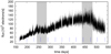 |
Fig. 1. Analysed Kepler light curve of MV Lyr with shaded regions roughly showing two intervals with constant flux. The vertical blue lines divide the light curve into 12 subsamples used for the shot profile evolution calculation in Sect. 4.3. |
3. Superimposed shot profile
We performed a similar superimposed shot profile analysis as presented by Negoro et al. (1994). Our work is motivated by the use of this technique to Kepler data of the AGN W2R 1926+42 performed by Sasada et al. (2017). Our technique, which is slightly different, has two steps: the peak identification and the flare extension selection. For the former we used a simple condition that a light curve point is identified as a peak if Npts points to the left and Npts points to the right have lower fluxes than the tested point. The second step is the flare extension selection in order to not superimpose a declining branch of one flare with a rising branch of the adjacent flare, and vice versa. For this purpose a flare is identified as Nptsext = Npts/2 points to the left and Nptsext = Npts/2 to the right from the peak point. We performed some further tests which we present below, but this algorithm is the most secure approach to average individual flares.
After the flare selection we performed a simple averaging of the flare points and the resulting averaged flux minimum was subtracted from all averaged points. All flares with rare individual null points were excluded from the averaging process. It would be best to choose a short interval of the light curve with more or less constant flux (e.g. the first shaded area in Fig. 1), but this would result in a flare number that is too low. Therefore, we first used the rising part of the light curve from the beginning to day 439 (until the beginning of the second shaded area in Fig. 1). A fainter division of the light curve yields a lower flare number, but is suitable for an evolution study.
Finally, the long-term trend visible in Fig. 1 has no effect on the results. De-trended data yield the same profile because any long-term trend is negligible within the time extent of a single shot. Moreover, Kepler data are not uniformly spaced because of barycentric correction. Our averaging method assumes evenly spaced data, and every shot is handled separately. Since the central points (peaks) are aligned, any time step modification has an effect within half of a single shot. The largest time extent of a single shot used in this work is of 3.3 h, which is extremely short for a time step variation due to barycentric correction. A simple test with evenly re-sampled data using linear interpolation yields almost the same shot profile with negligible differences. However, we always get lower variance when we use linear interpolation; the interpolated point is always between the two real points, both the time and flux values. The latter is the reason why we prefer the original data.
Three examples of the superimposed averaged shot profile are shown on Fig. 2 with inset panels as a zoom. The shot profile consists of a central spike and apparent side lobes on both sides. Another structure is visible at approximately −2100 s (in the middle and bottom panel). The best would be to have a Nptsext parameter as large as possible to get a large time extension before and after the central spike to see all of the details. But, as seen in Fig. 2, a higher Npts with larger time extension yields lower a flare number, resulting in a more noisy shot profile. Therefore, some compromise is needed between the flare profile time extension and the data scatter.
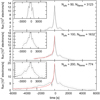 |
Fig. 2. Superimposed shot profiles using three different values of Npts resulting in different flare numbers Nflares and flare time extension. The inset panels are detailed views without the central spike to better visualize the side lobes. The solid black line represents the mean value, while the dotted thin line represents the standard error of the mean. The thick dashed (red) line is the power-law fit and the two arrows in the bottom panel show the interval excluded from the fitting process (see Sect. 7 for details). |
The presented technique is different from that used by Negoro et al. (1994) and Sasada et al. (2017). These authors superimposed well-resolved and isolated flares (see Fig. 4 in Sasada et al. 2017). However, in the MV Lyr Kepler data such well-resolved and isolated flares are not present, but many flares are superimposed instead. This is depicted in Fig. 3. Different Npts were used to select the flares. In the case of Npts = 10 the majority of flares are well resolved and have a spiky shape. However, this Npts value is too low to study any expanded structures because of the short time extension. When increasing the Npts parameter, the resolved flares become too complicated and many superimposed flare maxima can be present in the selected data interval. The averaging process keeps the central spike and smooths out all randomly present adjacent flares maxima and keep only the real structures. This is also important in uncertainty determination. We used the standard error of the mean instead of the standard deviation because the latter would describe the data scatter from superimposed adjacent flares maxima and not the intrinsic profile uncertainty.
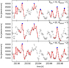 |
Fig. 3. Example of selected flares (red solid lines) using different Npts values. The open circles represent the light curve data, while the solid (blue) circles represent the maxima. |
We performed a simple reality test to prove that the detected substructures are real to exclude any doubts due to possible numerical artefacts. We took the largest shot profile (Npts = 200) from Fig. 2 and constructed a synthetic light curve with the same duration and sampling as the observed light curve. We superimposed 100 000 flares in random to construct the light curve. The resulting artificial flux was rescaled to be comparable with observed light curve characteristics (mean flux and rms). Such a process is not ideal because the superposition of flares is a shot noise model that does not satisfy all typical features of the real light curves. Our goal however is not reproduction of real data, but to test whether the superposition of many flares keeps the original shot profile. This shows that every structure present in the input shots is present in the resulting averaged profile with secure Npts selection. This is an important test because of the characteristics of the light curve, where many adjacent flares maxima are superimposed in the selected flare region. The presence of such adjacent maxima does not influence the result.
The test results are shown as red lines in Fig. 4. We used a selection criterion of Npts = 50, but we used different Nptsext values to investigate the flare extension. The averaged shot profile has the same structure, i.e. a central spike with side lobes and a possible hump at −2100 s for Nptsext ≥ 50. However, the increasing and decreasing trend of the flare wing is critical. This behaviour depends on the parameter Nptsext, i.e. whether it is lower or equal to Npts. With Nptsext = 2 × Npts the flare wings start to change trend at approximately −3500 s and 5000 s; they rise instead of decline and vice versa. For an extreme value of Nptsext = 6 × Npts this false trend is clearer, which stabilizes itself above 10 000 s.
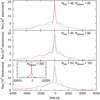 |
Fig. 4. Superimposed shot profiles from simulated light curves using different extraction parameters Nptsext (dashed red line). We used the input shot profile (solid black line) for the synthetic light curve construction from bottom panel of Fig. 2. |
This test suggests that Nptsext can be set up as equal to Npts, but as already mentioned to avoid any undetected artefacts resulting from superimposition (repetition of the same data) of adjacent flares we used Nptsext = Npts/2. The large quantity of Kepler data allows such waste.
Finally, when using a much simpler profile for input shots for the synthetic light curve construction (a simple spike without side lobes), only a profile similar to that used was obtained as the averaged profile. Therefore, the side lobes are real and are not artefacts.
4. Shot profile fitting
We concentrated our study on the central spike and the most dominant side lobes to quantitatively describe the detected profile. These features are well resolved even in shorter light curve subsegments where lower Npts is required to get larger flares quantity. We fitted these two features individually via the GNUPLOT2 software, yielding the fitted parameters with the standard errors.
4.1. Central spike
Sasada et al. (2017) fitted the central spike with two functions. The first was proposed by Abdo et al. (2010) to represent blazar flare profiles, and is written as
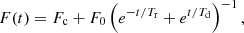 (1)
(1)
where t is time, Tr and Td are variation timescales of a rising and declining branch, respectively. The values Fc and F0 represent the constant level and the amplitude of the shots, respectively. The second fit used by Sasada et al. (2017) is written as
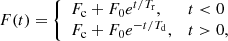 (2)
(2)
with the same parameter meanings as in Eq. (1). Figure 5 shows both fits as red lines performed from3 −285 s to 285 s. Clearly, the case described by Eq. (2) is better4 and even describes the profile well. The most expressive difference is visible near the central spike maximum, where the model following Eq. (1) does not describe the pointed profile well. The fitted timescales with the ratios Tr/Td are listed in Table 1.
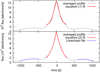 |
Fig. 5. Fits of the individual shot profile components. The black line indicates Npts = 50 case with best resolution from top panel of Fig. 2. The red line indicates the exponential fit following Eqs. (1) or (2) and the blue lines indicate the Lorentzian fits using Eq. (3). |
Fitted timescales of rising and declining parts of the central spike and the corresponding timescale ratios.
4.2. Side lobes
We further investigated the time location of the side lobes. For this purpose we fitted the side lobes with a Lorentz function
 (3)
(3)
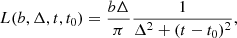 (4)
(4)
where Ψ is the flux, a and b are constants, Δ is the half width at half maximum, t is time from the peak, and t0 is the searched side-lobe time location, to the visually selected lobes, yielding the times of −639.1 ± 13.1 and 736.2 ± 6.4 s for the rising and declining lobe, respectively. The time distance between the lobes is approximately 1375 s and the fits are shown as blue lines in Fig. 5.
4.3. Components evolution
For the profile evolution we used light curve subsamples as they come from the Kepler archive (the intervals are marked as blue lines in Fig. 1), and the fitted profiles are shown in the left panel of Fig. 6. The evolution of fitted parameters as timescales and side-lobe peak times are depicted in Figs. 7 and 8. We used two regimes: first, the fitted parameter versus mean flux of the data subsample and second, the fitted parameters versus the central time of the light curve subsample.
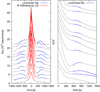 |
Fig. 6. Left panel: individual shot profiles (Npts = 50) from light curve subsamples with individual component fits. The time evolution is from bottom to top. The lowest profile has the original flux values, while every next profile is offset by 2000 el. s−1 vertically. Right panel: same as left panel but derived using ACF. |
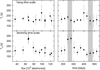 |
Fig. 7. Timescales of the central spike evolution as functions of the averaged flux (left panels) and light curve segment time (right panels). The shaded areas in the right panels correspond to the shaded areas in Fig. 1. |
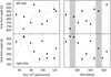 |
Fig. 8. Same as Fig. 7, but for side-lobe central times. The dashed lines represent the same, but derived from the ACF in Sect. 5 for comparison. |
For the spike fitting we changed the fitted time intervals when the fits run away significantly from the shot profile, otherwise we used the same time interval as in Sect. 4.1. This change of the fitting interval was needed in the four last cases with the largest fluxes because the amplitude of the central spike was too high. The fitted timescales with the ratios for individual light curve subsamples are listed in Table 1.
Inspecting the Fig. 7 we see nothing significant when studying the flux or time evolution, except two points in both bottom panels. The declining timescale Td shows a significant value deviation for fluxes of approximately 70 el. s−1. This value corresponds to the local flux plateau shown as shaded area in Fig. 1. The second flux plateau at the maximum flux of the light curve, where the trend changes from rising to declining, does not show this Td deviation.
Finally, the majority of averaged shot profiles have discernible side lobes. However, the first profile with the lowest flux has missing side lobes, while the rising lobe of the 11th case is too noisy for any relevant fit. The resulting side-lobe central times in Fig. 8 are too scattered to draw any conclusion from the flux or time evolution.
5. Auto-correlation
Another way how to study the fast variability shape or the shot profile is the use of the auto-correlation function (ACF). However, the ACF is an even/symmetric function, which is not suitable to study asymmetric profiles because the location of the two side lobes is represented by only one feature in the ACF. In any case, it is worth investigating this approach to get another reality test of the shot profile method and derived shot substructures.
To calculate the ACF we need evenly spaced data, which is a problem using the whole Kepler light curve. We replaced every rare null point or larger gap by linear interpolation. An ACF of the data used in Fig. 5 is depicted in Fig. 9. There is a significant lobe located at 657.25 ± 4.07 s shown as the Lorentz fits as in Sect. 4.2. Apparently, this value is very close to the average (687.7 s) of both side-lobe locations derived by the shot profile method. This suggests the reality of the substructures. Furthermore, there is a weak but noticeable hump at 2200 ± 4 s in the ACF (enhanced by linear de-trending in the inset panel of Fig. 9). This feature5 location is similar to the left hump in the shot profile in bottom panel of Fig. 2.
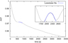 |
Fig. 9. Same as in Fig. 5, but derived using ACF and for larger timescales (lags). The inset panel shows ACF region between 1400 and 2900 s after linear de-trending to enhance the hump structure fitted by Lorentzian. |
The right panel of Fig. 6 shows the ACF evolution as an analogy to the left panel. The first (bottom) ACF that does not show a side lobe and the fourth ACF with a clearly enhanced side lobe are worth noting. Both results are consistent with the shot profile evolution. Figure 8 compares the ACF lobe location evolution with those derived from the averaged shot profile method. The first view does not suggest a perfect or strong correlation, but Kendall rank correlation coefficients for the rising and declining side lobes are 0.87 and 0.69, respectively. This suggests a significant correlation (even strong correlation in the rising lobe case) of the results derived from both methods.
The uneven character of the Kepler data must also be tested in the case of the ACF. Using linearly interpolated data such as in the shot profile calculation, we get the same ACF features, but the values are slightly, vertically offset toward higher values. Therefore, we used original data like in Sect. 3.
Finally, the presence of the side lobes, showing similar behaviour and evolution compared to the shot profile method, is additional proof that the detected features are real and the averaged shot profile method is working well.
6. Power density spectra
6.1. Simulated PDSs
In Sect. 4.2 we showed that the two side lobes are located at times −639.1 ± 13.1 and 736.2 ± 6.4 s. These side lobes correspond to two waves of a 687.7 ± 7.3 s period (average value) with a corresponding frequency of log(f/Hz) = −2.837 ± 0.004. The latter suggests a similarity with frequency components detected in PDSs studied by Scaringi et al. (2012b). To study the meaning of this similarity, we simulated light curves with the simple shot noise process6 using the shot profile from Fig. 2; we used the shot profile with the largest timescale (bottom panel). We performed PDS analysis of this synthetic light curves following Dobrotka et al. (2015) to get the closest approach to the PDSs presented in Scaringi et al. (2012b). We selected light curve samples with duration of 25 d. We divided these samples into five equal subsamples and for every subsample we calculated a periodogram using the Lomb-Scargle (Scargle 1982) algorithm, transformed the periodogram into log-log scale, averaged all 5 log-log7 periodograms, and binned the averaged periodogram into equally spaced bins to arrive at the PDS estimate. The Fourier transform would be ideal for a perfectly equidistant simulated light curve, but for the later purpose in which we calculated the PDSs from the Kepler data we chose Lomb-Scargle as ideal for non-equidistant data. Kepler data have a lot of gaps and spurious null points or intervals of null points. Therefore, we used the Lomb-Scargle method for all PDS estimates to get equivalent results. Finally, Lomb-Scargle is often used for the study of PDS in equidistant data as well (see e.g. Shahbaz et al. 2005).
Three examples of simulated PDSs are shown in Fig. 10. The clearest pattern in all the three cases is the break frequency or PDS component at approximately log(f1/Hz) = −3. Another common well-resolved hump is seen at around log(f2/Hz) = −3.4. Lower frequencies are rather flat and scattered without any dominant pattern. Some power excess is noticeable at approximately log(f3/Hz) = −3.7, and the lower end of the PDS shows a common power decrease toward low frequencies from approximately log(f4/Hz) = −4.2. But these are of low significance. We compared these simulated PDSs with frequencies8 detected in Kepler data from Table 1 (see also Fig. 4) of Scaringi et al. (2012b). The two highest frequencies from Kepler data clusters around the clearest PDS patterns at f1 and f2, and a possible match is noticeable in the f4 case. There is no obvious or systematic correlation of f3 with the observed histogram, even the presence of any power excess close to f3 in the simulations is not certain (middle panel). Therefore, we can conclude that at least the two highest PDS components detected by Scaringi et al. (2012b) are directly seen in the averaged shot profile.
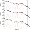 |
Fig. 10. PDSs calculated from simulated light curve subsamples. The points are averaged means with the standard error of the mean as vertical lines. The vertical shaded area shows the frequencies of two points with a small power deviation at log(f/Hz) = −2.46 and −2.41 representing a potential high frequency PDS component. The solid red lines represent the histogram of frequencies detected in Kepler data from Table 1 of Scaringi et al. (2012b). |
Moreover, two deviated points are seen at log(f/Hz) = −2.46 and −2.41 in the simulated PDSs (indicated as the vertical shaded area in Fig. 10). If real, these suggest a new high frequency PDS component that has not been detected so far with a characteristic frequency in between the two values.
6.2. Kepler PDSs
The two deviated points with very stable values motivated us to search for this feature in the real data. We first divided the whole studied Kepler light curve (Fig. 1) into 25 day subsamples and performed the same Lomb-Scargle analysis as in Sect. 6.1. Figure 11 shows these PDSs with vertical dotted lines showing the two frequencies.
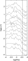 |
Fig. 11. PDSs calculated from Kepler light curve. The whole light curve in Fig. 1 is divided into equal 25 day segments and every PDS represents the corresponding segment; the first PDS is at the bottom. The vertical shaded area shows the frequencies of expected power excess between log(f/Hz) = −2.46 and −2.41. |
Not every PDS from the observed data shows a power deviation at the frequency of the expected power excess, but some cases are promising. However, the significance is very low, which is expected also from simulations. The Poissonian noise in the real data makes the detection even harder.
6.3. XMM-Newton PDS
As a next step we searched for the same component in XMM-Newton data. We took the EPIC pn light curve from Dobrotka et al. (2017). We performed the same Lomb-Scargle calculation as in the previous cases, but we re-binned the averaged periodogram into larger bins (interval of 0.1 in log scale), and with a minimum of five averaged points (top panel of Fig. 12). We did this to smooth strongly the periodogram to see the main trends and strongest features. This revealed a considerably deviated point at approximately log(f/Hz) = −2.43 (exactly between the two frequencies from simulated PDSs).
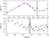 |
Fig. 12. Top panel: PDS of XMM-Newton data with broken power-law fit, and mean (solid red line) PDS value with 1σ intervals (red dashed lines) from 100 simulations. Bottom panel: PDS with higher resolution and broken power-law fit plus Lorentzian. The shaded area shows the region of expected power excess between log(f/Hz) = −2.46 and −2.41. |
As a reality test, we simulated light curves using the method of Timmer & Koenig (1995). This method uses an input PDS to generate noisy light curves. For this purpose we fitted the low resolution PDS with a broken power law9 (blue thick solid line) to get PDS estimate describing the main trends. The simulated light curves have the same length, sampling, mean flux value and variance as the observed data. We added a Gaussian noise to the curve to fit well the highest frequency part of the observed PDS. The solid red line in the top panel of Fig. 12 is the mean value of 100 simulated light curves, and the dashed curves represent the 1σ interval. Apparently, the anomalous point deviates from the main trend with amplitude slightly larger than the 1σ interval.
This power deviation can represent a new high frequency PDS component. We increased the PDS resolution from 0.1 to 0.025 with a minimum number of averaged points 3 to search for its characteristics. We fitted the high resolution PDS with a broken power law plus a Lorentzian (Eq. (4); with L = log(p), t = f and t0 = f0). The fit is depicted in the bottom panel of Fig. 12 and the fitted characteristic frequency is log(f0/Hz) =  .
.
7. Discussion
We performed an analysis of the superimposed shot profile of the Kepler data of the nova-like system MV Lyr based on the original idea of Negoro et al. (1994). We investigated the details of the shot profile and its time evolution, and we searched for links between the shot profile and the multi-component PDS of the Kepler data.
7.1. Shot profiles from Kepler data
This work is motivated by a similar analysis of Kepler data of the blazar W2R 1926+42 performed by Sasada et al. (2017). The authors found a very similar shot profile as that depicted in Fig. 2 of this work, i.e. an asymmetric central spike with two side lobes. The fitting of the central spike in MV Lyr yields a timescale ratio Tr/Td of 0.73 ± 0.14, which agrees well with the ratio of 0.70 ± 0.03 for the blazar W2R 1926+42 (from Table 1 of Sasada et al. 2017). Furthermore, Sasada et al. (2017) subdivided the light curve into subsamples yielding timescale ratios of 0.40−1.01. This compares to 0.47−1.17 in the case of MV Lyr (Table 1). The weighted means for the former and latter is 0.63 ± 0.11 and 0.84 ± 0.13, respectively. Apparently, the asymmetry of the central spike characterized by these ratios is very similar for both objects. The spike has a fast rise and slow decline. A similar asymmetry in MV Lyr was suggested by Scaringi et al. (2014). However, the authors reported the opposite, i.e. the flare is rising more slowly than it is falling. This asymmetry is derived from the Fourier analysis and it is valid for the highest break frequency at log(f/Hz)= − 3 in the PDS. This discrepancy requires a detailed comparison between the PDS and the shot features (see below).
The timing characteristics of the central spike can be estimated from the two timescales Tr and Td (from Table 1). Following Negoro et al. (2001) these timescales correspond to knees in the PDS with corresponding frequencies of 1/(2πT). Sasada et al. (2017) found a break frequency of log(f/Hz) = −4.39 in the PDS of W2R 1926+42, which is very close to the rising and declining timescales of the central spike of the blazar data. Therefore, this frequency represents the central spike of the mean profile. Following Scaringi et al. (2012b) the observed PDS of MV Lyr has the highest frequency component of approximately log(f/Hz) = −3. Based on the previous analogy, such frequency should be seen in the shot profile. Calculating the characteristic frequencies using Tr and Td we get values of log(f/Hz) = −3.01 and −3.15, respectively. Apparently, the dominant central spike of the averaged shot profile corresponds to the dominant PDS component in MV Lyr.
Furthermore, in Sect. 6 we show that a pattern with a frequency of log(f/Hz) = −2.42 is generated in the simulated PDS (Fig. 10). This motivated us to search for this feature in the real data. While the Kepler PDSs show the expected power excess with very low significance, the excess in the re-analysed XMM-Newton PDS is more convincing. A corresponding timescale is of 263 s. Such a structure is not identifiable in our shot profile, but such a short timescale can corresponds to the narrowest peak of the central spike.
Moreover, the side-lobe maxima in MV Lyr are located at times −639.1 ± 13.1 and 736.2 ± 6.4 s from the zero. As already mentioned these side lobes correspond to two wave-lengths of a 687.7 ± 7.3 s length wave with corresponding frequency of log(f/Hz) = −2.837 ± 0.004. The latter is very close to the dominant PDS feature at log(f/Hz) = −3, which clearly contributes to this PDS feature. Apparently all the fine structures of the shot profile have corresponding components in the PDS. However, while the individual components are blending and are seen as just one dominant PDS feature or are indistinguishable owing to low resolution, the shot profile is able to recognize them separately. This can explain the discrepancy between asymmetry of the dominant central spike detected in this work and the opposite asymmetry derived by Scaringi et al. (2014), i.e. the latter reported positive skewness for a dominant PDS break frequency at approximately log(f/Hz) = −2.7. This is close to the side-lobe frequency of log(f/Hz) = −2.8, while for the lower frequencies of log(f/Hz) = −3.01 and −3.15 related to the central spike the time skewness is negative (see Fig. 1 of Scaringi et al. 2014). For even lower frequencies the skewness returns to positive values. Such negative skewness agrees with the slower decay as seen in the central spike, and the positive skewness for the side lobes and lowest frequencies (approximately log(f/Hz) < −3.4) agree with the reverse behaviour. In Fig. 13 we directly compare the rising and decaying parts of the mean profile, and apparently the overall decaying part representing the lowest frequencies is faster. In this case, the shot profile behaviour does not contradict the Scaringi et al. (2014) finding. Both the frequencies and skewness suggest that the finding by these authors, based on the most dominant PDS feature, does not refer to the central spike.
To compare the side-lobe location in the AGN and CV, we estimated their relative positions using timescale ratios. The ratio of the rising timescale of the central spike Tr to the time coordinate of the rising side lobe (t0 in Eq. (4)) yields a value of 0.26 ± 0.03 for MV Lyr, while it is 0.31 ± 0.05 for the declining timescale Td and location of the declining side lobe. To get equivalent ratios in W2R 1926+42 we performed a rough estimate of the side-lobe time locations from Fig. 5 in Sasada et al. (2017). The corresponding values are −0.3 ± 0.05 and 0.3 ± 0.05 d, where the uncertainty is half of the axis resolution of 0.1 d. The ratios are 0.14 ± 0.02 and 0.20 ± 0.03 for the rising and declining part, respectively. When comparing the ratios of both objects we can conclude that they are different. Therefore, in spite of their similarity, the shot profile of W2R 1926+42 is not just a time amplification of the MV Lyr shot profile.
7.2. PDS structure
MV Lyr was already studied in detail, yielding the discovery of a multi-component PDS (Scaringi et al. 2012b). Numerical modelling of the highest dominant component supports a sandwiched model origin, i.e. the fast variability with a frequency of log(f/Hz)≃ − 3 is generated by an inner evaporated hot corona (geometrically thick and optically thin disc) with a standard geometrically thin and optically thick accretion disc below (Scaringi 2014). Such a corona radiates in X-rays and this radiation is reprocessed by the geometrically thin accretion disc resulting in detected optical radiation. This was confirmed by the XMM-Newton observation by Dobrotka et al. (2017), yielding a presence of the log(f/Hz)≃ − 3 component in an X-ray PDS10. This suggests a very low mass accretion rate typical for a dwarf novae in quiescence, which is not typical for a high state of a nova-like system resembling a dwarf nova in outburst. This dilemma was explained by an evaporated corona having very low density yielding a low mass accretion rate with a standard geometrically thin disc below with a mass accretion rate typical for a nova-like system in a high state.
Finally, the presence of the new high frequency PDS component at log(f/Hz) = −2.42 in XMM-Newton data suggests a coronal or boundary layer origin at log(f/Hz) = −3.0 and −3.4, as mentioned above. This is an important conclusion because it rules out all other potential sources of flickering, such as a hot spot11, an outer disc, or the interaction of an overflowing stream from the secondary with the disc. However, this only relates to the radiation source. The initiating fluctuation can be generated elsewhere, even in an outer disc or a hot spot (see below in this section).
While X-ray detection localizes the radiation source, the localization of the fluctuation is not easy. The basic idea is that every characteristic frequency or PDS component has its own origin in the disc. This hypothesis was studied by Dobrotka et al. (2015) using simulations, yielding a complex model of the accretion flow from the more active outer disc rim toward the central inner disc. If the studied fast variability would be a simple superposition of several different signals, they should be independent. Mainly fluctuations from outer parts of the disc would be indiscernible in the studied X-ray data. However, our finding from Sect. 6 suggests a different concept based on single signal with a complex flare profile with substructures having their own characteristic timescales. Such a conclusion is clear from Fig. 10, in which at least two most dominant previously detected PDS components are present. If the flickering activity were a superposition of different and independent signals, all patterns would be independent and not appearing simultaneously as seen in the averaged shot profile.
Furthermore, such a simple additive process is not real because of a typical rms-flux relation. This relation has a linear trend (Scaringi et al. 2012a for MV Lyr) in general, which is typical for multiplicative processes. Therefore, the signals generated by different disc structures cannot be independent and a correlation is expected. Following the propagating mass accretion fluctuation model the mass accretion variability at outer radii is propagating toward the center and influences the variability characteristics in inner regions. This means that a large mass accretion fluctuation at the outer disc propagates inward and generates further fluctuations on local viscous timescales which decrease inwards. All events with various timescales generated by this initial outer event must be correlated and yield an energy release at the boundary layer. This could be the reason why the complicated averaged shot profile has so much information, only part of which is generated in the corona; this corona contribution is manifested as the highest frequency components. The rest could have their origin in different or outer disc parts. A definitive conclusion on whether such a complex shot profile is a result of propagating accretion fluctuations is beyond the scope of this paper, and we leave the idea to other colleagues specialized in theoretical modelling. Finally, the presence of the several detected PDS components in simulated light curves using the observed profile supports the reality of these PDS components because they are directly seen in the averaged shot profile.
7.3. Shot profile evolution
The shot profile evolution represented in Figs. 7 and 8 does not show anything worth discussing except the declining timescale Td of the central spike. The data show more or less constant values within the errors except two values during the first flux plateau in the light curve around day 260, where a constantly rising trend experienced a short interval of more or less constant flux. The first idea is that this different Td appears during the trend change, but there is a second plateau or trend change around day 460 at which we do not see similar Td deviation.
Another idea emerges, but it is just a speculation. The monotonic flux rise until the maximum around day 460 is slow. Such flux increase can be generated by a mass transfer increase from the secondary, resulting in increasing the mass accretion rate through the disc and generating a flux rise. The subsequent flux decrease after day 460 can be explained by a similar reason, i.e. a mass transfer decrease. Such mass transfer variations are believed to be the origin of the long-term variability of nova-like systems of VY Scu types (see Warner 1995 for a review). However, if the first plateau is accompanied by the central spike Td deviation, while the next plateau is not, this suggests a different origin of the two intervals with the constant fluxes. In this concept the variation in the mass transfer rate from the secondary generated the flux plateau around day 460, but an unknown fluctuation or instability appeared around day 260 and generated a temporal flux trend deviation.
Some other information concerning the time evolution of the shot profile can be taken from ACF calculations by Kraicheva et al. (1999). The authors used ground observations of MV Lyr obtained in 1992 and 1993. The side lobes present in ACFs in Fig. 6 at approximately 700 s from the zero (0.19 h) are also present in Fig. 4 of Kraicheva et al. (1999), but the location is variable. This implies that the average shot profile possibly changes on timescales of days, i.e. on a shorter timescale than that of our samples shown in Fig. 6.
7.4. Comparison to W2R 1926+42 and fluctuating mass accretion flow
After our tests and the Monte Carlo simulations of Sasada et al. (2017) we have concluded that the detected shot profile and the similarities with the blazar W2R 1926+42 are real. It is beyond the scope of this paper to offer a physical explanation of the detailed profile, but the very similar profiles suggest a common origin. The similarity is not only qualitative, but also quantitative. The timescale ratios Tr/Td in both objects are very comparable, but on the other side the location of the side lobes relative to the central spike timescales are different. Both objects are accretion powered but are very different in nature. This makes the similarities even more surprising.
Sasada et al. (2017) first excluded geometrical effects in W2R 1926+42 based on changes in viewing angle in a bent jet or gravitational lensing as the variability origin. The authors argued with the asymmetric central spike. In the case of MV Lyr we can exclude any gravitational lensing phenomena and the jet presence is questionable12. Some further jet-related rough cooling timescales and emission region size estimates by Sasada et al. (2017) did not yield satisfying results. However, Sasada et al. (2017) concluded that the rapid variations are plausibly explained by the particle-acceleration scenario in the jet. This is questionable and less probable in MV Lyr because this CV has an outflow (Dobrotka et al. 2017; Balman et al. 2014), but it is more wind-like.
As a fast variability origin in MV Lyr Scaringi (2014) proposed propagating accretion rate fluctuations in the disc. This unstable mass flow in the (central) disc also feeds any (central) outflow. Therefore, it is easy to imagine that the source of variability is the fluctuating mass accretion rate unstably feeding all inner structures such as the central corona (a radiation source in MV Lyr) or a jet (a radiation source in blazar). Within this scenario, every characteristic of the mass accretion rate fluctuation or unstable accretion in the (inner) disc should propagate into the corona and/or jet and modulate the radiation there, yielding similar radiation behaviour. However, following recent radio observations of NGC 1275 by Giovannini (2018), the jet does not need to be generated necessarily in the very central regions. The authors found a broad jet with a transverse radius larger than 250 gravitational radii at only 350 gravitational radii from the core. The jet can be launched from the disc in that case and every mass accretion fluctuation can naturally be seen in the mass ejection.
Such interpretation needs further observational or theoretical studies. In the former case, the direct X-ray observations should say whether the optical blazar activity corresponds to the corona X-ray activity, while in the latter case, the same PDS modelling as carried out by Scaringi (2014) should test whether the observed blazar timescales are equivalent to the propagating mass accretion rate fluctuations.
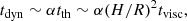
However, some rough timescale estimates can provide a clue about whether there is any connection between the observed flare durations. The basic timescales (dynamical tdyn, thermal tth and viscous tvisc) in the disc are connected as follows (see e.g. King 2008):
 (5)
(5)
where H and R are the height scale of the disc and distance from the center, respectively. The value tdyn is estimated from circular orbits as follows:
 (6)
(6)
where G and M are the gravitational constant and white dwarf (black hole) mass, respectively. Finally, a realistic estimate for tvisc is written as
 (7)
(7)
Translating this into an equation for a radius R estimate we get
![Mathematical equation: $$ \begin{aligned} R \sim \left(GM\,t_{\rm visc}^2\,[\alpha (H/R)^2]^2 \right)^{1/3} . \end{aligned} $$](/articles/aa/full_html/2019/11/aa35198-19/aa35198-19-eq9.gif) (8)
(8)
Following Scaringi (2014) the PDS component at log(f/ Hz)≃ − 3 is generated by an inner evaporated hot corona. Re-analysed X-ray data in this work suggest that also the central spike with a higher corresponding frequency of log(f/Hz)≃ − 2.42 in the PDS is generated in this corona, i.e. tvisc ≃ 263 s. The primary mass in MV Lyr is of about 0.73 M⊙ (Hoard et al. 2004) and α(H/R)2 = 0.705 (Scaringi 2014). The resulting corona radius roughly estimated from Eq. (8) is 1.5 × 1010 cm, which is close to the value of  cm derived by Scaringi (2014).
Performing the same calculus for the blazar with the black hole mass approximately 107 M⊙ (Mohan et al. 2016) or 107.8 M⊙ (Marconi & Hunt 2003), and the central spike timescale with the duration of 24547 s (from Sasada et al. 2017, log(f/Hz) = −4.39), the Eq. (8) yields a value of 7.4 × 10¹³ or 1.4 × 1014 cm for the corona radius13. The typical corona in an AGN is of approximately 10 Swarzschild radii (Liu et al. 2017), i.e. 10 × 2MG/c2 ≃ 3 × 1013 cm (c being the speed of light) or ≃2 × 1014 cm for both black hole mass estimates, respectively. Therefore, the values derived from the Eq. (8) are comparable to 10 Swarzschild radii.
Both timescale estimates from the CV and the blazar are well explainable by the viscous processes in the central geometrically thick corona. If the estimated tvisc in the blazar is proportional to the plasma injection time into the jet, this could explain the above-mentioned connection between the viscous processes in the corona and radiation fluctuations within the jet.
7.5. Comparison to Cygnus X-1 and aperiodic mass accretion model
Kepler data are not the only data suitable for the superimposed shot profile study. The same was made by Negoro et al. (2001) in the case of Ginga data of Cyg X-1. The shot profile of this XRB in X-rays has a similar shape as the two optical shot profiles discussed in this paper, i.e. a central spike with two humps, one before (at −1.85 s from zero) and one after (at 0.96 s from zero) the spike. The timescales are much shorter than those of the other two systems in which the central spike have durations of the order of 0.1−1 s (see Table 1 or Fig. 1 in Negoro et al. 2001). These timescales were estimated by two superimposed exponential functions; the shortest timescale (center of the spike) rises more gradually, but the longer timescale behaves in the same way as in the case of MV Lyr and W2R 1926+42, i.e. having a declining part of the central spike more gradual where Tr/Td = 0.72/1.13 = 0.64 ± 0.02. This value is comparable to both previously discussed objects.
The variability profile of Cyg X-1 can be derived from skewness measurement such as in the MV Lyr case described in Sect. 7.1. Maccarone & Coppi (2002) and Scaringi et al. (2014) analysed RXTE data of this XRB and found skewness behaviour comparable to the shot profile shape in Ginga data, i.e. timescales from approximately 1 s have negative skewness which agrees with the above derived Tr/Td ratio (slower decay)14. The skewness returns back to positive values for larger timescales of approximately 5 s (comparable to the largest 0.15 Hz sine function in Fig. 1 of Negoro et al. 2001) describing the overall rising and decaying trend, which has a profile behaviour similar to MV Lyr.
Using the same Tr and Td values and side-lobe locations at −1.85 ± 0.01 and 0.96 ± 0.03 s for the rising and declining side lobe, respectively, we can estimate the relative side-lobe location represented by the timescale ratios as in Sect. 7.1. The ratios are 0.39 ± 0.01 and 1.18 ± 0.05 for the rising and declining part, respectively. Considering that the side-lobe locations were not stable and changed from −4 s to −1.85 s in Ginga 1987 and 1990 observations, respectively (Negoro 1995); the ratio in the rising part is comparable to the MV Lyr value of 0.26 ± 0.03.
All three discussed objects are accretion powered, and Negoro (1995) proposed a physical interpretation based on the unstable mass accretion rate within the disc, the so-called aperiodic mass accretion model. Following this model, clumps of accreting matter drift inwards releasing the gravitational energy in the form of a flickering flare. Negoro (1995) proposed the shape of the flare rising branch to be expressed as
 (9)
(9)
where A, τ and α are constants. The most important and sensible parameter is the power α. The author fitted this function to superimposed profiles of Cyg X-1 taken by Ginga in 1987 and 1990 and got α = 0.7 in both cases. We performed the same procedure in the case of MV Lyr with corresponding fits shown as red lines in Fig. 2. In the Npts = 200 case the fit did not describe the profile well, therefore we excluded the two humps from the fitting process; between −2550 and −400, the interval is indicated by two arrows in bottom panel of Fig. 2. Both fits yield α = 0.7 as in Cyg X-1 Ginga data.
The similarity supports the same physical process. We talk about the aperiodic mass accretion in Cyg X-1 and propagating mass accretion fluctuations in MV Lyr. These mass accretion fluctuations within the central corona can be imagined as a clump of accreting matter drifting inwards and releasing gravitational energy.
7.6. Possible contamination and other detections
Borisov (1992) and Skillman et al. (1995) studied ground data of MV Lyr and concluded possible presence of a superhump period of 0.1379 d with a corresponding frequency of log(f/Hz) = −4.08. The latter authors however concluded that their data were less strongly supportive than the former authors data. The search for such coherent periodicity is beyond the scope of this paper, but we performed a very rough attempt to search for this signal and did not succeed. However, such a frequency is much lower than the highest frequency components of log(f/Hz) = −3.0 and −2.4, representing the side lobes and the central spike which we study in this work in detail. Therefore, any contamination by a superhump (if present) is irrelevant.
Dobrotka et al. (2016) studied the rms-flux relation of two SU UMa systems observed by Kepler. While V1504 Cyg shows the typical linear rms-flux relation, V344 Lyr does not. However, the latter exhibit superhump activity and if the flickering has a linear rms-flux relation, the additional superhump flux must deform this linearity. The authors showed with simple simulations how superhump activity with varying amplitude deformed the linearity and they obtained a very comparable rms-flux relation to the observed data. This implies that if any significant superhump activity is present in MV Lyr, the rms-flux relation must differ from linearity. But this is not the case (Scaringi et al. 2012a). If still present, it must be of very small amplitude or significance. Borisov (1992) reported a 4% amplitude.
Finally, Borisov (1992) and Skillman et al. (1995) together with Kraicheva et al. (1999) found a quasi-periodic oscillation at a period near 47 min. The corresponding frequency of log(f/Hz) = −3.45 is in perfect agreement with one PDS component detected by Scaringi et al. (2012b) in the optical Kepler data and by Dobrotka et al. (2017) in the X-ray XMM-Newton light curve. This power excess is also seen in the simulations (Fig. 10) based on the averaged shot profile method in this paper. Therefore, all findings are consistent.
7.7. Method
Finally, we note that the averaged shot profile method is a not generally accepted approach. However, this method gives us a new way to investigate fast variability and has some advantages compared to the standard PDS or ACF methods.
First is the fact that the shot profile method uses only fragments of the light curve. If the calculation of the ACF requires evenly spaced data, this can be problematic if the light curve has many interruptions. Interpolation of the data by anything is already bringing false information and can affect the results. The shot profile method uses only the flares, i.e. short fragments of the data.
Another advantage is seen when comparing both panels of Fig. 6. The left panel shows that the central spike is rising in amplitude with the average overall flux, while the side-lobe amplitudes are more or less stable. This behaviour not seen in ACF suggests that the central spike (the highest frequencies) is responsible for the rms-flux relation detected by Boeva et al. (2011) in ground observations and by Scaringi et al. (2012a) using the Kepler data.
Furthermore, some PDS components are directly seen in the shot profile. All the Fourier based methods are somehow abstract descriptions of the reality. The shot profiles directly show the phenomenon, such as components location, variability amplitudes, and any asymmetry. Mainly the latter is important as it is not seen in the ACF. As a consequence we detected similarity of the variability in MV Lyr and the blazar. Such similarity is hardly deducible from the PDSs. Finally, individual PDS components can have similar frequencies and be indistinguishable in the PDS, while they are seen as separate features in the shot profile.
Moreover, the detection of the new high frequency component was done thanks to the averaged shot profile and subsequent light curve and PDS simulations. Without the small power deviation of two PDS points based on the simulations we would not be motivated to search for the component in the real data. The advantage is that such a PDS is based on artificial light curves constructed with the averaged profile, where the whole noise is smoothed by the averaging process and only real features remain. Finally, this positive result certifies the harmlessness of the inappropriate shot noise model.
8. Summary and conclusions
The superimposed averaged shot profile of flickering activity in MV Lyr Kepler data shows a complex structure with a central spike and side lobes on both sides of the central spike. These various substructures correspond to a single dominant component in the PDS detected by Scaringi et al. (2012b). The standard PDS is not able to distinguish these substructures. We confirmed the reality of the features using a shot noise model. This approach is purely phenomenological because it does not fulfil all details of the underlying physics. Moreover, additional tests showed that Kepler data which is not evenly sampled because of barycentric correction has no effect on the results. Finally, the credibility of the shots is supported by timescale ratios of the rising and declining shot parts when compared to the skewness measurement of Scaringi et al. (2014).
Time evolution of these shots in MV Lyr does not show any significant evolution or correlation with the flux except during a short flux plateau. The declining timescale of the central spike increased during this time interval.
A very similar complex shot profile structure appears in Kepler data of the blazar W2R 1926+42 (Sasada et al. 2017) and in Ginga data of Cyg X-1 (Negoro et al. 1994, 2001). These object are very different in nature. The timescales of the rising and declining branches of the central spikes in the corresponding observations have very comparable ratios. Moreover, the rise of the shots in MV Lyr and Cyg X-1 follow a trend with the same power law (see Negoro 1995 for Cyg X-1 case). These similarities between the averaged shot profiles in the three very different objects in nature but powered by accretion imply a similar physical origin of the variability within the accretion process. The origin can be the same (propagating accretion rate fluctuations in the disc feeding the inner disc), but emitting regions can be different (the corona in MV Lyr and the jet in W2R 1926+42).
Finally, simple shot noise simulations using the averaged shot profile yield to the identification of another high frequency PDS component not identified so far. The component is noticeable with low significance in Kepler data but very clear in XMM-Newton EPIC pn light curve. The latter suggests that the radiation source is in the inner region of the disc, i.e. the corona or boundary layer.
If not prevented by strong magnetic field of the compact object.
The limits are chosen empirically.
The sum of residuals square is six times lower than with the Eq. (1).
This feature is of very low significance, but we do not use it for any analysis. Therefore, we do not investigate or discuss its credibility.
The same procedure as in Sect. 3.
Following Papadakis & Lawrence (1993) it is more suitable to average log(p) instead of power p.
 .
.
A power law is written as log(p) = a log(f) + b, where a is the power-low slope and b is the constant. Broken power law means that two different power laws are used below and above a break frequency.
XMM-Newton PDS also shows the second break frequency at log(f/Hz)≃ − 3.4 confirming the reality of the feature.
Interaction of disc edge with the plasma stream from the secondary.
Following thermal models, which describe jets generation by young stellar objects, the jets in CVs are not probable (Soker & Lasota 2004). However, it was recently shown that CVs are significant radio emitters, and synchrotron radiation is the emission mechanism making the presence of the jets possible (Coppejans et al. 2015, 2016).
Supposing the same α(H/R)2 parameter as in MV Lyr for a geometrically thick corona.
The skewness resolution is not sufficient for the shorter timescales of ∼0.1 s studied by Negoro et al. (2001).
Acknowledgments
AD was supported by the ERDF – Research and Development Operational Programme under the project “University Scientific Park Campus MTF STU – CAMBO” ITMS: 26220220179. HN was partially supported by Grants-in-Aid for Scientific Research 16K05301 from the Ministry of Education, Culture, Sports, Science and Technology (MEXT) of Japan.
References
- Abdo, A. A., Ackermann, M., Ajello, M., et al. 2010, ApJ, 722, 520 [NASA ADS] [CrossRef] [Google Scholar]
- Arévalo, P., & Uttley, P. 2006, MNRAS, 367, 801 [NASA ADS] [CrossRef] [Google Scholar]
- Balman, Ş., Godon, P., & Sion, E. M. 2014, ApJ, 794, 84 [NASA ADS] [CrossRef] [Google Scholar]
- Boeva, S., Bachev, R., Tsvetkova, S., et al. 2011, Bulg. Astron. J., 16, 23 [Google Scholar]
- Borisov, G. V. 1992, A&A, 261, 154 [NASA ADS] [Google Scholar]
- Borucki, W. J., et al. 2010, Science, 327, 977 [NASA ADS] [CrossRef] [PubMed] [Google Scholar]
- Bruch, A. 2015, A&A, 579, A50 [NASA ADS] [CrossRef] [EDP Sciences] [Google Scholar]
- Coppejans, D. L., Körding, E. G., Miller-Jones, J. C. A., et al. 2015, MNRAS, 451, 3801 [NASA ADS] [CrossRef] [Google Scholar]
- Coppejans, D. L., Körding, E. G., Miller-Jones, J. C. A., et al. 2016, MNRAS, 463, 2229 [NASA ADS] [CrossRef] [Google Scholar]
- Dobrotka, A., & Ness, J.-U. 2015, MNRAS, 451, 2851 [NASA ADS] [CrossRef] [Google Scholar]
- Dobrotka, A., Mineshige, S., & Ness, J.-U. 2014, MNRAS, 438, 1714 [NASA ADS] [CrossRef] [Google Scholar]
- Dobrotka, A., Mineshige, S., & Ness, J.-U. 2015, MNRAS, 447, 3162 [NASA ADS] [CrossRef] [Google Scholar]
- Dobrotka, A., Ness, J.-U., & Bajčičáková, I. 2016, MNRAS, 460, 458 [NASA ADS] [CrossRef] [Google Scholar]
- Dobrotka, A., Ness, J.-U., Mineshige, S., & Nucita, A. A. 2017, MNRAS, 468, 1183 [NASA ADS] [CrossRef] [Google Scholar]
- Giovannini, G., et al. 2018, Nat. Astron., 2, 472 [Google Scholar]
- Hoard, D. W., Linnell, A. P., Szkody, P., et al. 2004, ApJ, 604, 346 [NASA ADS] [CrossRef] [Google Scholar]
- King, A. 2008, New Astron. Rev., 52, 253 [NASA ADS] [CrossRef] [Google Scholar]
- Kotov, O., Churazov, E., & Gilfanov, M. 2001, MNRAS, 327, 799 [NASA ADS] [CrossRef] [Google Scholar]
- Kraicheva, Z., Stanishev, V., & Genkov, V. 1999, A&AS, 134, 263 [NASA ADS] [CrossRef] [EDP Sciences] [Google Scholar]
- Liu, B. F., Taam, R. E., Qiao, E., & Yuan, W. 2017, ApJ, 847, 96 [NASA ADS] [CrossRef] [Google Scholar]
- Lyubarskii, Y. E. 1997, MNRAS, 292, 679 [NASA ADS] [CrossRef] [Google Scholar]
- Maccarone, T. J., & Coppi, P. S. 2002, MNRAS, 336, 817 [NASA ADS] [CrossRef] [Google Scholar]
- Marconi, A., & Hunt, L. K. 2003, ApJ, 589, L21 [NASA ADS] [CrossRef] [Google Scholar]
- McHardy, I. 1988, Mem. Soc. Astron. It., 59, 239 [NASA ADS] [Google Scholar]
- Miyamoto, S., Kitamoto, S., Iga, S., Negoro, H., & Terada, K. 1992, ApJ, 391, L21 [NASA ADS] [CrossRef] [Google Scholar]
- Mohan, P., Gupta, A. C., Bachev, R., & Strigachev, A. 2016, MNRAS, 456, 654 [NASA ADS] [CrossRef] [Google Scholar]
- Negoro, H. 1995, PhD Thesis, Osaka University [Google Scholar]
- Negoro, H., Miyamoto, S., & Kitamoto, S. 1994, ApJ, 423, L127 [NASA ADS] [CrossRef] [Google Scholar]
- Negoro, H., Kitamoto, S., & Mineshige, S. 2001, ApJ, 554, 528 [NASA ADS] [CrossRef] [Google Scholar]
- Papadakis, I. E., & Lawrence, A. 1993, MNRAS, 261, 612 [NASA ADS] [CrossRef] [Google Scholar]
- Sasada, M., Mineshige, S., Yamada, S., & Negoro, H. 2017, PASJ, 69, 15 [NASA ADS] [CrossRef] [Google Scholar]
- Scargle, J. D. 1982, ApJ, 263, 835 [NASA ADS] [CrossRef] [Google Scholar]
- Scaringi, S. 2014, MNRAS, 438, 1233 [NASA ADS] [CrossRef] [Google Scholar]
- Scaringi, S., Körding, E., Uttley, P., et al. 2012a, MNRAS, 421, 2854 [NASA ADS] [CrossRef] [Google Scholar]
- Scaringi, S., Körding, E., Uttley, P., et al. 2012b, MNRAS, 427, 3396 [NASA ADS] [CrossRef] [Google Scholar]
- Scaringi, S., Körding, E., Groot, P. J., et al. 2013, MNRAS, 431, 2535 [NASA ADS] [CrossRef] [Google Scholar]
- Scaringi, S., Maccarone, T. J., & Middleton, M. 2014, MNRAS, 445, 1031 [NASA ADS] [CrossRef] [Google Scholar]
- Shahbaz, T., Dhillon, V. S., Marsh, T. R., et al. 2005, MNRAS, 362, 975 [NASA ADS] [CrossRef] [Google Scholar]
- Skillman, D. R., Patterson, J., & Thorstensen, J. R. 1995, PASP, 107, 545 [NASA ADS] [CrossRef] [Google Scholar]
- Soker, N., & Lasota, J.-P. 2004, A&A, 422, 1039 [NASA ADS] [CrossRef] [EDP Sciences] [Google Scholar]
- Sunyaev, R., & Revnivtsev, M. 2000, A&A, 358, 617 [NASA ADS] [Google Scholar]
- Timmer, J., & Koenig, M. 1995, A&A, 300, 707 [NASA ADS] [Google Scholar]
- Uttley, P., McHardy, I. M., & Vaughan, S. 2005, MNRAS, 359, 345 [NASA ADS] [CrossRef] [Google Scholar]
- Van de Sande, M., Scaringi, S., & Knigge, C. 2015, MNRAS, 448, 2430 [NASA ADS] [CrossRef] [Google Scholar]
- Vaughan, S., Edelson, R., Warwick, R. S., & Uttley, P. 2003, MNRAS, 345, 1271 [NASA ADS] [CrossRef] [Google Scholar]
- Warner, B. 1995, Cataclysmic Variable Stars, Cambridge Astrophysics Series (Cambridge: Cambridge Univ. Press), 28 [Google Scholar]
- Zamanov, R., Latev, G., Boeva, S., et al. 2015, MNRAS, 450, 3958 [NASA ADS] [CrossRef] [Google Scholar]
All Tables
Fitted timescales of rising and declining parts of the central spike and the corresponding timescale ratios.
All Figures
|
Fig. 1. Analysed Kepler light curve of MV Lyr with shaded regions roughly showing two intervals with constant flux. The vertical blue lines divide the light curve into 12 subsamples used for the shot profile evolution calculation in Sect. 4.3. |
| In the text | |
|
Fig. 2. Superimposed shot profiles using three different values of Npts resulting in different flare numbers Nflares and flare time extension. The inset panels are detailed views without the central spike to better visualize the side lobes. The solid black line represents the mean value, while the dotted thin line represents the standard error of the mean. The thick dashed (red) line is the power-law fit and the two arrows in the bottom panel show the interval excluded from the fitting process (see Sect. 7 for details). |
| In the text | |
|
Fig. 3. Example of selected flares (red solid lines) using different Npts values. The open circles represent the light curve data, while the solid (blue) circles represent the maxima. |
| In the text | |
|
Fig. 4. Superimposed shot profiles from simulated light curves using different extraction parameters Nptsext (dashed red line). We used the input shot profile (solid black line) for the synthetic light curve construction from bottom panel of Fig. 2. |
| In the text | |
|
Fig. 5. Fits of the individual shot profile components. The black line indicates Npts = 50 case with best resolution from top panel of Fig. 2. The red line indicates the exponential fit following Eqs. (1) or (2) and the blue lines indicate the Lorentzian fits using Eq. (3). |
| In the text | |
|
Fig. 6. Left panel: individual shot profiles (Npts = 50) from light curve subsamples with individual component fits. The time evolution is from bottom to top. The lowest profile has the original flux values, while every next profile is offset by 2000 el. s−1 vertically. Right panel: same as left panel but derived using ACF. |
| In the text | |
|
Fig. 7. Timescales of the central spike evolution as functions of the averaged flux (left panels) and light curve segment time (right panels). The shaded areas in the right panels correspond to the shaded areas in Fig. 1. |
| In the text | |
|
Fig. 8. Same as Fig. 7, but for side-lobe central times. The dashed lines represent the same, but derived from the ACF in Sect. 5 for comparison. |
| In the text | |
|
Fig. 9. Same as in Fig. 5, but derived using ACF and for larger timescales (lags). The inset panel shows ACF region between 1400 and 2900 s after linear de-trending to enhance the hump structure fitted by Lorentzian. |
| In the text | |
|
Fig. 10. PDSs calculated from simulated light curve subsamples. The points are averaged means with the standard error of the mean as vertical lines. The vertical shaded area shows the frequencies of two points with a small power deviation at log(f/Hz) = −2.46 and −2.41 representing a potential high frequency PDS component. The solid red lines represent the histogram of frequencies detected in Kepler data from Table 1 of Scaringi et al. (2012b). |
| In the text | |
|
Fig. 11. PDSs calculated from Kepler light curve. The whole light curve in Fig. 1 is divided into equal 25 day segments and every PDS represents the corresponding segment; the first PDS is at the bottom. The vertical shaded area shows the frequencies of expected power excess between log(f/Hz) = −2.46 and −2.41. |
| In the text | |
|
Fig. 12. Top panel: PDS of XMM-Newton data with broken power-law fit, and mean (solid red line) PDS value with 1σ intervals (red dashed lines) from 100 simulations. Bottom panel: PDS with higher resolution and broken power-law fit plus Lorentzian. The shaded area shows the region of expected power excess between log(f/Hz) = −2.46 and −2.41. |
| In the text | |
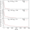 |
Fig. 13. Same as Fig. 2, but with directly compared rise and decay parts of the mean profiles. |
| In the text | |
Current usage metrics show cumulative count of Article Views (full-text article views including HTML views, PDF and ePub downloads, according to the available data) and Abstracts Views on Vision4Press platform.
Data correspond to usage on the plateform after 2015. The current usage metrics is available 48-96 hours after online publication and is updated daily on week days.
Initial download of the metrics may take a while.