| Issue |
A&A
Volume 631, November 2019
|
|
|---|---|---|
| Article Number | A122 | |
| Number of page(s) | 15 | |
| Section | Astrophysical processes | |
| DOI | https://doi.org/10.1051/0004-6361/201834921 | |
| Published online | 05 November 2019 | |
Overshooting in simulations of compressible convection
1
Georg-August-Universität Göttingen, Institut für Astrophysik, Friedrich-Hund-Platz 1, 37077 Göttingen, Germany
e-mail: This email address is being protected from spambots. You need JavaScript enabled to view it.
2
ReSoLVE Centre of Excellence, Department of Computer Science, Aalto University, PO Box 15400 00076 Aalto, Finland
Received:
19
December
2018
Accepted:
4
September
2019
Abstract
Context. Convective motions that overshoot into regions that are formally convectively stable cause extended mixing.
Aims. We aim to determine the scaling of the overshooting depth (dos) at the base of the convection zone as a function of imposed energy flux (ℱn) and to estimate the extent of overshooting at the base of the solar convection zone.
Methods. Three-dimensional Cartesian simulations of hydrodynamic compressible non-rotating convection with unstable and stable layers were used. The simulations used either a fixed heat conduction profile or a temperature- and density-dependent formulation based on Kramers opacity law. The simulations covered a range of almost four orders of magnitude in the imposed flux, and the sub-grid scale diffusivities were varied so as to maintain approximately constant supercriticality at each flux.
Results. A smooth heat conduction profile (either fixed or through Kramers opacity law) leads to a relatively shallow power law with dos ∝ ℱn0.08 for low ℱn. A fixed step-profile of the heat conductivity at the bottom of the convection zone leads to a somewhat steeper dependency on dos ∝ ℱn0.12 in the same regime. Experiments with and without subgrid-scale entropy diffusion revealed a strong dependence on the effective Prandtl number, which is likely to explain the steep power laws as a function of ℱn reported in the literature. Furthermore, changing the heat conductivity artificially in the radiative and overshoot layers to speed up thermal saturation is shown to lead to a substantial underestimation of the overshooting depth.
Conclusions. Extrapolating from the results obtained with smooth heat conductivity profiles, which are the most realistic set-up we considered, suggest that the overshooting depth for the solar energy flux is about 20% of the pressure scale height at the base of the convection zone. This is two to four times higher than the estimates from helioseismology. However, the current simulations do not include rotation or magnetic fields, which are known to reduce convective overshooting.
Key words: turbulence / convection
© ESO 2019
1. Introduction
Convective mixing in stars has important consequences, for example, in early and late phases of stellar evolution and for the diffusion of light elements. Furthermore, stellar differential rotation (e.g. Rüdiger 1989) and dynamos (e.g. Moffatt 1978; Krause & Rädler 1980; Brandenburg & Subramanian 2005) owe their existence to turbulent fluid motions. The efficiency of mixing in convective and radiative layers in stars differs greatly. The former are vigorously mixed on a timescale much shorter than the evolutionary timescale of the star. Thus it is of great interest to be able to predict where effective convective mixing occurs. The greatest uncertainty in this respect is the amount of overshooting from convection zones (CZ) to adjacent radiative layers.
Stellar structure and evolution models most often apply some variant of the mixing length (ML) model of Vitense (1953) to describe convection. These models are completely local and do not allow overshooting. Non-local extensions to ML models (e.g. Shaviv & Salpeter 1973; Schmitt et al. 1984; Skaley & Stix 1991) yield estimates of overshooting, but the validity of the ML approach has been questioned (e.g. Renzini 1987). More advanced closures of convection based on Reynolds stress (e.g. Xiong 1985; Deng et al. 2006; Garaud et al. 2010; Canuto 2011) are physically more consistent but challenging to implement (see, however, Zhang et al. 2012; Zhang 2013). Furthermore, testing and validation of the Reynolds stress models, for example, by comparison to three-dimensional numerical simulations, is still in its infancy (e.g. Kupka 1999; Snellman et al. 2015; Cai 2018).
A seemingly attractive option to study overshooting is to solve the governing equations directly by means of three-dimensional simulations. Numerical simulations of convection have been used to estimate the overshooting depth in numerous studies (e.g. Hurlburt et al. 1986, 1994; Roxburgh & Simmons 1993; Singh et al. 1995, 1998; Saikia et al. 2000; Brummell et al. 2002; Ziegler & Rüdiger 2003; Rogers et al. 2006; Tian et al. 2009; Pratt et al. 2017; Brun et al. 2017; Hotta 2017; Korre et al. 2019). Early studies indicated overshooting of the order of a pressure scale height at the base of the CZ, which is an order of magnitude more than typical estimates from helioseismology (e.g. Basu 1997). The difference between these studies and the Sun is that the energy flux imposed in the simulations is typically much greater than the corresponding solar flux. This leads to higher convective velocities in the simulations and to an overestimation of the overshooting. Scaling laws, based on the relation of convective velocities with the energy flux, arise in analytic models of overshooting (e.g. Zahn 1991; Rempel 2004) and predict a reduction of the overshooting depth as a function of decreasing flux. The primary aim of the current study is to establish these relations from carefully controlled numerical experiments.
Compressible simulations with realistic solar energy flux are hampered by the disparity of the acoustic and dynamical timescales, or by a low Mach number, in the deep parts of the CZ. According to ML arguments, the enthalpy flux 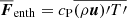 , where cP is the heat capacity at constant pressure, ρ is the density, u is the convective velocity, and T is the temperature, and the apostrophes (overbar) denote fluctuations (averages) that can be approximated as
  (Brandenburg 2016). Assuming that
  , it is possible to construct a normalised energy flux (e.g. Brandenburg et al. 2005),
 (1)
(1)
The last approximation is justified by the fact that the factor ϕ has been reported to be in the range 4 − 20 (Brandenburg et al. 2005; Brandenburg 2016), whereas convection carries only a fraction of the total flux in the lower part of the solar CZ (see, e.g. the solar model of Stix 2002). Using solar values at r0 = 0.71 R⊙, where R⊙ = 7 × 10⁸ m is the solar radius, 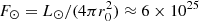 W m−2, where L⊙ = 3.84 × 1026 W is the solar luminosity, ρ ≈ 200 kg m−3, and cs ≈ 200 km s−1, the normalised flux at the base of the solar CZ is
 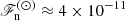 . Thus the Mach number in the deep CZ is about 10−4. This leads to a short time-step due to the high sound speed and to prohibitively long integration times (e.g. Kupka & Muthsam 2017). Although anelastic methods (e.g Gough 1969) bypass the acoustic time-step problem at solar luminosity, any simulation attempting to do this self-consistently would need to be run for a Kelvin–Helmholtz time to achieve thermal saturation. This is not feasible for solar parameters without resorting, for example, to arbitrarily changing the heat conductivity in the radiative layer (e.g. Brun et al. 2017) with current and any foreseeable supercomputers (e.g. Kupka & Muthsam 2017).
Recently, Hotta (2017) presented results from numerical simulations of fully compressible convection where the overshooting depth was computed from a range of two orders of magnitude in the input flux. He reached values of ℱn = 5 × 10⁻⁷, which is at the limits of current numerical feasibility, and obtained a power law 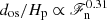 for the overshooting depth dos. This led Hotta (2017) to estimate that the overshooting at the base of the solar CZ is about 0.4% of the pressure scale height, or roughly 200 km. Earlier numerical studies (e.g. Singh et al. 1998; Tian et al. 2009) have reported results that suggest a similar steep dependency of dos on ℱn.
Here these studies are revisited by a set-up where the heat conductivity is self-consistently computed using the Kramers opacity law. This set-up allows the depth of the CZ to dynamically adapt to changes in the thermodynamic state of the system (Käpylä et al. 2019a) and to produce a smooth transition between convective and radiative layers (Brandenburg et al. 2000; Käpylä et al. 2017). Furthermore, a significantly broader range of imposed flux values is covered than in any of the previous studies. Moreover, particular care is taken to isolate the effect of the input flux by performing models where the supercriticality of convection, degree of turbulence, and effective thermal Prandlt number are approximately constant as the flux varies. An effort is made to link to the earlier studies of Singh et al. (1998) and Tian et al. (2009) by targeted sets of simulations probing the influence of subgrid scale entropy diffusion on convection and the resulting overshooting depth. Finally, a critical assessment of some of the modeling choices of Hotta (2017) is presented.
The PENCIL CODE1 was used to produce the simulations. At the core of the code is a switchable finite-difference solver for partial differential equations that can be used to study a wide selection of physical problems. In the current study a third-order Runge–Kutta time-stepping method and centred sixth-order finite differences for spatial derivatives are used (cf. Brandenburg 2003).
2. The model
The Kramers set-ups used in the current study are similar to those in Käpylä et al. (2017). The equations for compressible hydrodynamics
 (2)
(2)
 (3)
(3)
![Mathematical equation: $$ \begin{aligned}&T \frac{\mathrm{D} s}{\mathrm{D} t} = -\frac{1}{\rho } \left[\boldsymbol{\nabla \cdot } \left(\boldsymbol{F}_{\rm rad} + \boldsymbol{F}_{\rm SGS}\right) \right] + 2 \nu \boldsymbol{\mathsf{S }}^2 + \Gamma _{\rm cool}, \end{aligned} $$](/articles/aa/full_html/2019/11/aa34921-18/aa34921-18-eq12.gif) (4)
(4)
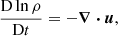
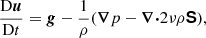
are solved, where D/Dt = ∂/∂t + u ⋅ ∇ is the advective derivative, ρ is the density, u is the velocity,  is the acceleration due to gravity with g > 0, p is the pressure, T is the temperature, s is the specific entropy, and ν is the constant kinematic viscosity. Furthermore, Frad and FSGS are the radiative and turbulent subgrid scale (SGS) fluxes, respectively, and Γcool describes cooling at the surface (see below). [BOLD]S is the traceless rate-of-strain tensor with
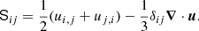 (5)
(5)
An optically thick fully ionised gas is considered, where radiation is modelled through diffusion approximation. The ideal gas equation of state p = (cP − cV)ρT = ℛρT applies, where ℛ is the gas constant, and cV is the specific heat at constant volume. The radiative flux is given by
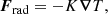 (6)
(6)
where K is the radiative heat conductivity. Two qualitatively different heat conductivity prescriptions are considered, where K either has a fixed profile K(z) or is a function of density and temperature, K(ρ, T). In the latter case, K is given by
 (7)
(7)
where σSB is the Stefan-Boltzmann constant and κ is the opacity. κ is assumed to obey a power law
 (8)
(8)
where ρ0 and T0 are reference values of density and temperature. Equations (7) and (8) combine into
 (9)
(9)
Here a = 1 and b = −7/2 are used, which correspond to the Kramers opacity law for free-free and bound-free transitions (Weiss et al. 2004). Heat conductivity consistent with the Kramers law was first used in convection simulations by Brandenburg et al. (2000).
Owing to the strong depth dependence of the radiative diffusivity, χ = K/(cPρ), additional turbulent SGS diffusivity is used in the entropy equation to keep the simulations numerically feasible. Here the SGS flux is formulated as
 (10)
(10)
where  is the fluctuation of the specific entropy. The overbar indicates horizontal averaging here and in what follows. The coefficient
  is constant in the whole domain. FSGS has a negligible contribution to the net horizontally averaged energy flux, such that
  . The current SGS formulation is similar to those used in Käpylä et al. (2007, 2019a), and Brown et al. (2010), for example.
The cooling at the surface is described by
 (11)
(11)
where Γ0 is a cooling luminosity, T = e/cV is the temperature where e is the internal energy, and where Tcool = Ttop is a reference temperature corresponding to the fixed value at the top boundary.
2.1. Geometry, and initial and boundary conditions
The computational domain is a rectangular box where zbot ≤ z ≤ ztop is the vertical coordinate, where zbot/d = −0.45, ztop/d = 1.05, and where d is the depth of the initially isentropic layer (see below). In a few runs the domain extends to deeper layers such that zbot/d = −0.75 to accommodate deeper overshooting. The horizontal coordinates x and y run from −2d to 2d. The horizontal size of the box is thus LH/d = 4, and the vertical extent Lz/d is either 1.5 or 1.8.
The initial stratification consists of three layers. Two configurations of the three-layer set-up are considered here: in the first set-up (hereafter P2I), the two lower layers are polytropic with polytropic indices n1 = 3.25 (zbot/d ≤ z/d ≤ 0) and n2 = 1.5 (0 ≤ z/d ≤ 1). The uppermost layer above z/d = 1 is initially isothermal. This layer mimics a photosphere where radiative cooling is efficient. The choice of n1 is motivated by fact that in the special case where the temperature gradient in the corresponding hydrostatic state is constant, the solution is a polytrope with index 13/4; see Barekat & Brandenburg (2014) and Appendix A of Brandenburg (2016). Assuming that an extended stable layer forms at the bottom of the domain, its stratification is close to the hydrostatic solution (see, e.g. Käpylä et al. 2019a). This, however, can only be confirmed a posteriori because the depth of the convective layer is not pre-determined in the cases where the Kramers opacity law is used. In the second set-up (hereafter P3) all three layers are polytropic with indices (n1, n2, n3)=(2, 1.5, 1.5). In these cases the radiative diffusion in the uppermost layer is enhanced and no explicit cooling is applied. This configuration is the same as in Singh et al. (1998) and was chosen to accommodate comparisons with that study. The choice of n2 = 1.5 for the thermal stratification in the middle layer comes from the expectation that the convectively unstable layer is nearly isentropic in the final statistically saturated state. The initial velocity follows a Gaussian-noise distribution with an amplitude of about  .
.
The horizontal boundaries are periodic, and on the vertical boundaries, impenetrable and stress-free boundary conditions are imposed for the flow such that
 (12)
(12)
The temperature gradient at the bottom boundary is set according to
 (13)
(13)
where Fbot is the fixed input flux and Kbot(x, y, zbot) is the value of the heat conductivity at the bottom of the domain. On the upper boundary a constant temperature T = Ttop, coinciding with the initial value, is assumed.
2.2. Units, control parameters, and simulation strategy
The units of length, time, density, and entropy are given by
![Mathematical equation: $$ \begin{aligned}[x] = d,\quad [t] = \sqrt{d/g},\quad [\rho ] = \rho _0,\quad [s] = c_{\rm P}, \end{aligned} $$](/articles/aa/full_html/2019/11/aa34921-18/aa34921-18-eq27.gif) (14)
(14)
where ρ0 is the initial value of the density at z = ztop. The models with Kramers heat conductivity are fully defined by choosing the value of the kinematic viscosity ν, the gravitational acceleration g, the values of a, b, K0, ρ0, T0 and the SGS Prandtl number
 (15)
(15)
along with z-dependent cooling profile f(z). The values of K0, ρ0, and T0 are subsumed into a new variable  that is fixed by assuming the radiative flux at zbot to equal Fbot in the initial state. The profile f(z) = 1 above z/d = 1 and f(z) = 0 below z/d = 1, connecting smoothly over the interface over a width of 0.025d. Furthermore,
  sets the initial pressure scale height at the surface, thus determining the initial density stratification. All of the current simulations have ξ0 = 0.054.
In runs where a fixed profile of heat conductivity is used, the profile K(z) is needed instead of specifying  . In these cases the value of K at z = zbot is fixed similarly as was done for
  in the Kramers cases. In these cases the initial profile of the Prandtl number based on the radiative heat conductivity
 (16)
(16)
where χ(z)=K(z)/cPρ(z), sets the relative importance of viscous to temperature diffusion. We note that in general Pr = Pr(x, t) because ρ = ρ(x, t). In cases where K has a piecewise constant profile, it can be represented in terms of polytropic indices  , which refer to a corresponding non-convective hydrostatic solution. Starting the simulations from such solutions for the thermodynamic quantities is, however, impractical especially if the value n2 is far away from the final convective state, which is always close to the adiabatic value of 1.5. Thus these indices typically differ from those used to initialise the thermal variables (see also Brandenburg et al. 2005). The heat conductivities in the different layers are connected through
 (17)
(17)
where i and j refer to any of the three layers.
The dimensionless normalised flux is given by
 (18)
(18)
where ρbot and cs, bot are the density and the sound speed, respectively, at zbot in the initial non-convecting state.
The input energy flux determines the overall convective velocity realised in the simulations via  , see Eq. (1) and Käpylä et al. (2019b). Thus if only ℱn were changed, the relative importance of the diffusion coefficients, measured by Reynolds and Péclet numbers, would change as well. To eliminate these dependences, and to be able to concentrate solely on the effects of varying input flux, the viscosity and SGS entropy diffusion are scaled proportional to
  . In addition to changing the diffusion coefficients, the cooling luminosity Γ0 at the surface is also scaled proportionally to ℱn. The input flux itself is varied by changing the overall magnitude of K such that the value at the bottom is given by Kbot = −Fbot/(∂T/∂z)zbot. Furthermore, the degree of supercriticality of convection, measured by a Rayleigh number, and the Prandtl number, describing the ratio of viscosity to thermal diffusion, will affect the properties of convection and overshooting if they are allowed to vary. The current choice of the dependency of ν and
  on ℱn, however, eliminates these dependences such that the supercriticality and effective Prandtl numbers are nearly constant over the range of ℱn considered here. This is discussed in detail in Sect. 4.1.
In addition to the explicit viscosity, SGS, and radiative diffusion, the advective terms in each of the Eqs. (2)–(4) are written in terms of a fifth-order upwinding derivative with a hyperdiffusive sixth-order correction where the diffusion coefficient depends locally on the flow, see Appendix B of Dobler et al. (2006).
2.3. Diagnostics quantities
The following quantities are outcomes of the simulations that can only be determined a posteriori. These include the global Reynolds and SGS Péclet numbers,
 (19)
(19)
where urms is the volume-averaged rms velocity, and k1 = 2π/d is an estimate of the largest eddies in the system. Typically  in the CZ in most of the current simulations. Furthermore, χ has a strong depth dependence due to the density stratification. Thus it is useful to define Reynolds and effective Péclet numbers separately for the overshoot zone,
 (20)
(20)
where all quantities are taken from the base of the CZ, z = zCZ, with  being the mean (horizontally averaged) radiative diffusivity, and where kOZ = 2π/dos is a wavenumber based on the depth of the overshoot layer dos. Similarly, an effective Prandtl number can be defined as
 (21)
(21)
Precise definitions of zCZ and dos are given in Sect. 3.
To assess the level of supercriticality of convection, radiative and SGS Rayleigh numbers are defined as
 (22)
(22)
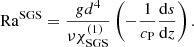 (23)
(23)
Supercriticality of convection is roughly determined by min(RaRad, RaSGS). Both quantities vary as functions of height and are quoted near the surface at z/d = 0.85 for all models. Conventionally, the Rayleigh number in the hydrostatic non-convecting state is one of the control parameters. This is still true for the cases with fixed K profile in the current study, but in the runs with Kramers conductivity, the convectively unstable layer in the hydrostatic case is very thin and confined to the near-surface layers (Brandenburg 2016). Thus the Rayleigh numbers are quoted from the thermally saturated and statistically stationary states.
The path in parameter space taken here is artificial in that in real fluids, there is no SGS diffusivity (RaSGS = 0) and any change in the flux would be reflected by the then decisive radiative Rayleigh number. For example, a system where Pr is fixed 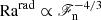 . However, taking this path severely limits the computationally feasible range of ℱn because the Reynolds and Péclet number also increase in proportion to ℱn and the resolution requirements quickly become prohibitive.
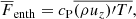
Contributions to the vertical energy flux are
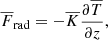 (24)
(24)
 (25)
(25)
 (26)
(26)
 (27)
(27)
 (28)
(28)
Here the primes denote fluctuations and overbars horizontal averages. The total convected flux (Cattaneo et al. 1991) is the sum of the enthalpy and kinetic energy fluxes:
 (29)
(29)
The radiative flux can be written in terms of the mean double-logarithmic temperature gradient  as
as
 (30)
(30)
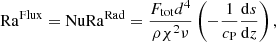
where cP∇ad = cP(1 − 1/γ)=ℛ, and g = |g|. Above, ∇ is the actual temperature gradient realised in the system. Now it is possible to define the total flux and the flux transported by adiabatic stratification as
 (31)
(31)
where ∇rad is a hypothetical radiative gradient in the absence of convection and Ftot = Fbot. The ratio of the total-to-adiabatic flux is the Nusselt number (e.g. Brandenburg 2016),
 (32)
(32)
In the current set-up the Nusselt number is fixed from the outset for cases with a static profile of  . This is because the total flux imposed at the lower boundary is proportional to
  . In the cases where Kramers conductivity is used,
  can evolve but the change in the Nusselt number is not very large; see, for example, Table 1. The behaviour of Nu is different in cases where fixed temperature is imposed at both boundaries (e.g. Yadav et al. 2016; Gastine et al. 2016) because the total flux is no longer in direct proportion with the heat conductivity.
Summary of the runs with smoothly varying profiles of K.
3. Definitions of CZ and overshooting
To characterise the different layers, the nomenclature introduced in Käpylä et al. (2017) is used, although with somewhat differing definitions. The CZ is defined to be the part of the domain where  , whereas in the overshoot zone (OZ) Fconv < 0. This is motivated by the work of Deng & Xiong (2008), who used a similar definition but employed
  instead of
  . A definition of the overshooting depth based on
  was also used in Käpylä et al. (2017). However, because the kinetic energy flux carries a substantial fraction of the energy, it is natural to include it in the definition of the CZ. The bottom of the CZ is denoted by zCZ.
The mean overshooting depth zOS is taken to be the position where the horizontally averaged  drops below 1% of its value at zCZ. Various earlier studies have used a similar definition (Hurlburt et al. 1986, 1994; Singh et al. 1995, 1998; Brummell et al. 2002). In most of the previous studies the location of the bottom of the CZ is assumed to be fixed by the initial conditions. Here this assumption is relaxed and zCZ is computed from the simulation data using the definition given above. The values of zOS and zCZ are obtained by linear interpolation from the grid points closest to the respective transitions. Furthermore, zCZ and zOS are functions of time. The overshooting depth is defined as
 (33)
(33)
where ⟨⋯⟩t denotes a time average over the statistically stationary part of the time series. Error estimates for dos are obtained by dividing the time series into three equally long parts and considering their largest deviation from the time average over the whole time series as the error.
The radiative zone (RZ) is defined as the region below zOS, and the buoyancy zone (BZ) is where  and
and  . Finally, the Deardorff zone (DZ) is characterised by a formally stable stratification with a positive vertical mean entropy gradient (
 ) and
) and  ; see, Tremblay et al. (2015). In this layer, the convective energy transport is dominated by a non-local non-gradient contribution to the enthalpy flux introduced by Deardorff (1961, 1966); see also Brandenburg (2016) and Käpylä et al. (2017). Such layers have been reported by various authors from simulations (e.g. Chan & Gigas 1992; Roxburgh & Simmons 1993; Tremblay et al. 2015; Korre et al. 2017; Bekki et al. 2017; Karak et al. 2018; Nelson et al. 2018). Furthermore, the union of OZ, DZ, and BZ is referred to as the mixed zone (MZ).
4. Results
Four main sets of simulations, denoted as K, P, S, and DS were conducted, see Tables 1–3. The sets are named after their heat conductivity prescriptions: in Set K, the Kramers law is used to compute the heat conductivity. In Set P, a static profile corresponding to the heat conductivity computed according to the Kramers law in the initial state of the simulation is used. Set S employs a static step profile of heat conductivity, K = K(z). These three sets correspond to Runs K, P, and S of Käpylä et al. (2017). Additionally, Sets Kh and Sh are the otherwise the same as Sets K and S, but lower viscosity and SGS entropy diffusion were used. These runs were branched off from corresponding thermally saturated snapshots from runs in Sets K and S, respectively. In Sets DS, DSS1, and DSS2 a double-step profile for K, similar to that in Singh et al. (1998), was used. In Set DS  and in Set DSS1 (DSS2) the SGS diffusion is included with
  . Runs DS5 and DS5h were the same except for the grid resolution to study numerical convergence of the results. Finally, in Set R the explicit diffusivities ν and
  were varied while all other parameters were kept fixed using Run K5 as a progenitor, see Table 4. Sets DS, DSS1, and DSS2 used the P3 set-up, and the remaining sets were initialised with the P2I set-up.
Summary of the runs with a fixed step profile of K.
Summary of the runs with a double-step profile for K.
4.1. Basic characterisation of the solutions
Typical flow patterns for Runs R4 and R7 are shown in Fig. 1. The flow structure observed in various studies of stratified non-rotating convection is recovered with connected downflows near the surface merging into isolated plumes at larger depths (e.g. Stein & Nordlund 1989, 1998). The downflows are surrounded by broader upflows. In the majority of the current simulations the flows are at best mildly turbulent with Re ≈ 20…40 such as in Run R4 in the left panel of Fig. 1. However, the qualitative large-scale structure of convection does not change at higher resolutions and Rayleigh and Reynolds numbers, see the right panel of Fig. 1 for Run R7.
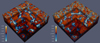 |
Fig. 1. Normalised vertical velocity |
Figure 2a shows the profiles of  from representative runs in each of the main sets K, P, S, and DS. The Kramers run K4 and the corresponding fixed profile model P4 have a smoothly varying profile as a function of height with very small values of
  near the surface. In the piecewise polytropic run S4, the profile of
  is characterised by constant values in the upper (z > 0) and lower (z < 0) layers (e.g. Hurlburt et al. 1986; Nordlund et al. 1992), which can be characterised by the ratios K2/K1 = K3/K1 = 4/17 ≈ 0.235. In Run DS5, K2/K1 = 2/85 ≈ 0.0333 and the uppermost layer above z/d = 1 has another constant value of
  corresponding to K2/K1 = 5/6. However, the transitions of
  between the layers are smoothed over a distance of 0.05d, due to which the value of
  corresponding to
  is achieved only near the upper surface.
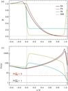 |
Fig. 2. Horizontally averaged and normalised heat conductivity |


The vertical profiles of Pr(z) and  are shown in Fig. 2b. The strong variation of Pr as function of depth is to be contrasted with the constant value of
  . Although Pr ∝ ℱn, it is still typically greater than unity at z/d = 0 in almost all cases, with the exception of a few runs with the highest values of ℱn (see Tables 1–4). This is in stark contrast to the solar CZ, where Pr ≪ 1 everywhere (e.g. Ossendrijver 2003). Numerical simulations with Prandtl numbers far different from unity are challenging numerically and render parameter studies infeasible. Thus an enhanced SGS diffusivity with
  of the order of unity was applied in most of the current simulations. In most of the current simulations the effective Prandtl number is dominated by the SGS diffusion.
Summary of the runs with varying ν and  .
.
Changing the input energy flux ℱn refers to varying the magnitude of  proportionally and thus χ ∝ ℱn. In combination with
  and the ML estimate −(Hp/cP)ds/dz =
  (Vitense 1953), this involves changing
  . This is to be contrasted with the SGS Rayleigh number, where χ is replaced by
  , which leads to RaSGS being independent of ℱn. These scalings are in accordance with the simulations, as can be seen from Fig. 3 for Sets Kh, DS, and DSS1. As mentioned earlier, the supercriticality of convection is determined roughly by min(RaRad, RaSGS). In the current simulations the SGS Rayleigh number is almost always smaller. This also means that with RaSGS≈ constant, the supercriticality of convection is also constant, and it is eliminated as an influence on the overshooting depth. For completeness, the flux-based Rayleigh number (e.g. Brun & Browning 2017)
 (34)
(34)
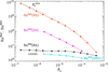 |
Fig. 3. Rayleigh numbers RaSGS (black) and RaRad (red) as functions of ℱn from Set Kh. The purple (magenta) line shows RaRad (RaSGS) from Set DS (DSS). The dotted lines show scalings expected from ML arguments. |
can be seen to vary as 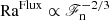 given the dependences above. We note that NuRaSGS is independent of ℱn.
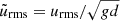
Figure 4 shows the dependence of the rms velocity within the CZ from all simulations except for those in Set R. The simulation results are close to a  dependence, with the coefficient of proportionality varying between 1.3 and 1.8. This is in agreement with ML estimates (e.g. Vitense 1953; Brandenburg et al. 2005; Brandenburg 2016) and earlier numerical findings (Brandenburg et al. 2005; Karak et al. 2015; Käpylä et al. 2019b).
 |
Fig. 4. Normalised rms velocity |


Results regarding the energy fluxes and force balance from representative runs from Sets K, S, and DS are shown in Fig. 5. The left panels show the contributions to the energy flux and the superadiabatic temperature gradient ∇ − ∇ad. The fluxes for Runs K4 and S4 in Fig. 5a and c are qualitatively similar to those of Runs K and S of Käpylä et al. (2017), respectively. The main difference to the latter is the treatment of the near surface layers; cooling layer in the present runs as opposed to an imposed entropy gradient in Käpylä et al. (2017), and the somewhat different values of ℱn; 1.8 × 10⁻⁵ here versus 9 × 10⁻⁶ in Käpylä et al. (2017). The subadiabatic Deardorff zone encompasses roughly a quarter of the MZ in Run K4, whereas in Run S4, the DZ is almost absent. The runs in Set DS differ from those in Set S in that convection transports almost all of the energy due to the lower K2/K1 ratio. Assuming that the temperature gradient in the final statistically saturated state is nearly adiabatic, the fraction of convective transport can be estimated from (cf. Brandenburg et al. 2005)
 (35)
(35)
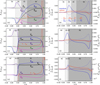 |
Fig. 5. Panels a, c, and e: total (black dash-dotted lines), convective (black), enthalpy (blue), kinetic energy (light purple), radiative (dark purple), and cooling (green) fluxes and the superadiabatic temperature gradient (red) from Runs K4, S4, and DS5, respectively. Panels b, d, and f: total averaged vertical forces (solid lines) and the power of the forces (dashed) on the upflows (red) and downflows (blue) from the same runs. The dotted lines in these panels show the corresponding viscous force and its power. The shaded areas indicate the BZ (darkest), DZ, and OZ (lightest) and the thick black line at the horizontal axis denotes the MZ. |
According to this expression, the convective flux transports 60% (96%) in the runs in Set S (DS). This is confirmed by the numerical results.
Figures 5b, d, and f show the horizontally averaged vertical total and viscous forces, 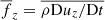 , and
, and  , respectively, and the resulting power of the forces (
 and
and  ) separately for the upflows (↑) and the downflows (↓) from Runs K4, S4, and DS5. The force balance in Run K4 (Fig. 5b), is very similar to the corresponding Run K in Käpylä et al. (2017), see their Fig. 2b. The downflows appear to adhere to the Schwarzschild criterion such that they are accelerated in the BZ and decelerated in the layers below. This is contrasted by the upflows that are accelerated in the stably stratified OZ and DZ and in the lower part of the BZ. As demonstrated in Käpylä et al. (2017), the upflows are not driven by the convective instability but are a result of matter displaced by the deeply penetrating downflows. In Run S4 the downflows are decelerated already in the lower part of the BZ whereas the force on the upflows is qualitatively similar to that in Run K4. The force balance in Run DS5 is qualitatively similar to that in Run S4 although the magnitude and details of the quantities differ. Interestingly the sign of the total force in the stably stratified layer near the surface is not reversed. The shallowness of the layer is likely contributing to this. Another aspect is the (true) overshooting from the CZ below. It can, however, be concluded that displacement of the matter due to the downflows is driving the upflows in the OZ and DZ also in Runs S4 and DS5. However, the superadiabatic temperature gradient has a local maximum at the bottom of the BZ in these cases, see Figs. 5c and e. Thus it is possible that the convective instability is contributing more to the upward acceleration in these cases. The viscous force is small in all cases and has a noticeable effect only in the near-surface layers above z/d = 0.75.
4.2. Dependence of overshooting on input flux
Reaching the solar value of ℱn is currently not possible due to the prohibitive time-step constraint and the long thermal adjustment time involved (e.g. Brandenburg et al. 2000; Kupka & Muthsam 2017). However, it is reasonable to assume that the overshooting depth scales with a power law as a function of ℱn (e.g. Schmitt et al. 1984; Zahn 1991). Thus it is in principle possible to estimate the extent of overshooting in the Sun provided that a sufficiently broad range of higher flux values are probed and their results are extrapolated to the solar case. A few such studies can be found in the literature (e.g. Singh et al. 1998; Tian et al. 2009; Hotta 2017).
One of the most restrictive modelling choices in the past has been the use of a static heat conduction profile that effectively enforces the layer structure of the simulation. This can be seen from Fig. 6a where the vertical coordinates of the bottoms of the convection (zCZ) and overshoot (zOZ) zones are shown as functions of ℱn. The results for zCZ from Sets S and Sh show that the interface between the CZ and OZ stays at the initial position at z = 0 for all values of ℱn. The runs in Sets DS, DSS1, and DSS2 behave similarly, although the bottom of the CZ is shifted downward from its initial position. For Sets K and Kh the depth of the CZ is generally reduced in comparison to Sets S and Sh. In these runs the depth of the CZ increases as ℱn decreases. This is contrasted by the results from Sets P where a Kramers-like, but static, profile of K is used (see Fig. 2): here zCZ is practically fixed in the current range of ℱn.
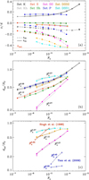 |
Fig. 6. Panel a: vertical (z) coordinates of the bottom of the CZ (zCZ, solid lines) and OZ (zOZ, dashed). The dotted red line indicates the bottom of the domain. Panel b: overshooting depth dos normalised by the pressure scale height Hp as a function of ℱn for Sets K (black), Kh (grey), P (blue), S (red), Sh (green), DS (purple), DSS1 (cyan), and DSS2 (orange). The purple diamond denotes Run DS5h. The dotted lines show approximate power laws from fits to simulation data; see Table 5. Panel c: comparison of Sets DS, DSS1, and DSS2 with the studies of Singh et al. (1998) (red) and Tian et al. (2009) (blue). |
Figure 6a shows that the location of the base of the OZ (zOZ) increases monotonically as a function of ℱn in all sets except for K and Kh. In Set DSS1 (DSS2) the overshooting extends to the lower boundary of the domain in the three (two) highest ℱn runs, rendering the results of these simulations unusable in the following analysis. The depth of the overshoot zone, dos, as a function of ℱn is shown in Fig. 6b. The results for Sets K, Kh, and P fall almost on top of each other. The data suggests two power laws:  for ℱn ≲ 10−5 and
  for ℱn ≳ 10−5; see Table 5. These results suggest that the overshooting depth is relatively insensitive to the choice of the heat conduction scheme if the profile of K at the base of the CZ is smooth. Furthermore, dos is consistently greater in Set Kh with higher Reynolds and SGS Péclet numbers than in the corresponding runs in Set K. This is because the current simulations have relatively modest Reynolds and Péclet numbers that are not in a fully turbulent regime. This aspect is studied in more detail in Sect. 4.3. At first glance, the data of Set Sh appear to be more consistent with a single power, and in Set S there appears to be a break around ℱn ≈ 10−5, such that the data points for lower values of ℱn lie below those of Set Sh. However, power-law fits for both full and partial ranges are consistent with a
  scaling within the error estimates; see Table 5.
Power-law exponents and standard mean errors from fitting  .
.
A similar set-up as in Singh et al. (1998) and Tian et al. (2009) is adopted in Sets DS, DSS1, and DSS2. The results of Set DS show a steep dependence of the overshooting on the input flux ( ), and Sets DSS1 with
  and DSS2 with
  are more in line with the other sets of simulations. The overshooting depth for the higher resolution Run DS5h is statistically consistent with that of Run DS5, although the overall velocities in these runs are somewhat lower. This is in particular reflected by the values of ReOZ and
  (seventh and eighth columns in Table 3). The fact that the results do not change drastically with resolution and that there is an apparently continuous transition as
  increases through Sets DSS1 and DSS2 to DS are indicative that the latter set of runs is sufficiently well resolved numerically. Figure 6c shows a comparison of the overshooting depths from Sets DS, DSS1, and DSS2 with the studies of Singh et al. (1998, their Table 1) and Tian et al. (2009, their Table 4). Both studies list the input fluxes Fb and values of density and pressure at the bottom of the domain (denoted here as ρb and pb). Thus the normalised flux in both cases is computed from ℱn = Fb/Fn, where
 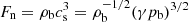 with
with  and γ = 5/3 has been assumed. The results of Singh et al. (1998) were obtained by a similar definition as used in the present study based on kinetic energy flux falling below a threshold fraction of its value at the base of the CZ. Their results are consistent with a
  scaling. On the other hand, Tian et al. (2009) obtained a very shallow dependence with this definition (
 ) and a much steeper one (
 ) when using a criterion based on the enthalpy flux falling below a threshold value of its absolute maximum in the OZ. It is unclear why the results from the two definitions used by Tian et al. (2009) deviate. Both definitions were tested with the current data and the results were found to be in fair agreement.
The drastic change from a steep power law in Set DS to the shallower power laws in Sets DSS1 and DSS2 is related to the difference in the diffusion of temperature fluctuations. Figure 7a shows that the effective Péclet numbers in OZ in all of these sets are comparable. However, as is shown in Sect. 4.3, the overshooting depth is insensitive to the Péclet number in this parameter range provided that the effective Prandtl number is not varied at the same time. The only difference between Sets DS and DSS1 and DSS2 is that in Set DS, the SGS entropy diffusion is omitted and thus the effective Rayleigh and Prandtl numbers vary as a function of ℱn, whereas in the latter two, they approach constant values for low ℱn, see Figs. 3 and 7b. Changing the effective Prandtl number leads to a dramatic change in the way convection transports energy in that the sound speed (temperature) fluctuations are enhanced over the velocity fluctuations with increasing Prandtl number, see Fig. 8a. This means that in Set DS the temperature fluctuations become increasingly more important in the enthalpy transport as ℱn (Pr) decreases (increases). This is immediately reflected in the overshooting depth as a smaller velocity fluctuation is required to carry the same flux. Figure 8b shows that in Set DSS1 the ratio of the temperature and velocity fluctuations remains practically constant as a function of ℱn. The break in the power law in Sets K and Kh can be understood similarly by the decreasing effective Prandtl number as ℱn increases.
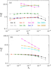 |
Fig. 7. Effective Péclet (panel a) and Prandtl (panel b) numbers at the base of the OZ. The vertical dotted line shows the approximate position of the break in the power laws in the overshooting depth in Fig. 6b. |
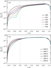 |
Fig. 8. Ratio of the rms vertical velocity and sound speed fluctuations from the runs in Set DS (panel a) and the runs in Set DSS (panel b). |
To connect the current findings to earlier studies, it is necessary to study the Prandtl number regimes explored by Singh et al. (1998), Tian et al. (2009), and Hotta (2017). In the two former studies a Smagorinsky viscosity νS was computed from the flow and entropy diffusion according to χS = PrSνS with a constant SGS Prandtl number of  was used. While this leads to the same average dependence of the diffusion coefficients as in the present study2, the SGS entropy diffusion in these studies was set explicitly to zero in radiative layers. This means that while the effective Prandtl number in the CZ is fixed, it increases in the overshoot layer as the flux is decreased. Thus the sensitivity to the Prandtl number discussed above is likely to explain the steep power laws found by Singh et al. (1998) and Tian et al. (2009). On the other hand, Hotta (2017) used a slope-limited diffusion method where the effective diffusion coefficients are also likely to be proportional to the gradients at small (grid) scales, that is, νsl ∝ u′Δx and χsl ∝ s′Δx. The velocity (entropy) fluctuations scale like
  (
( ) (cf. Käpylä et al. 2019b) and thus this would lead to
  scaling for the effective Prandtl number Prsl = νsl/χsl. Whether this simplistic picture of the effective Prandtl number with slope-limited diffusion when applied separately for the momentum and entropy equations is correct remains to be tested with numerical experiments. However, if it is true, then the effective Prandtl number is increasing with decreasing flux and is likely to contribute to the steep power law reported by Hotta (2017).
Furthermore, the studies of Singh et al. (1998), Tian et al. (2009), and Hotta (2017) all considered the bottom of the CZ to be fixed and given by the initial non-convecting state. Although all of these studies used a fixed profile for the heat conductivity, which fixes zCZ, it does not necessarily stay at the same position as in the initial state; compare, for example, the solid blue and red and green curves in Fig. 6a. This is particularly clear for Sets DS, DSS1, and DSS2 which are similar to the set-up of Singh et al. (1998). However, it is hard to assess whether such a systematic error is present in the results of Singh et al. (1998). In the simulations of Hotta (2017) a similar issue is also possible but it appears that this effect may be small (e.g. his Fig. 8).
Extrapolating from the current data of the Kramers runs (Sets K and Kh) to solar conditions suggests that the overshooting depth for  is 𝒪(0.2Hp). This is in better agreement with the constraints from helioseismology (e.g. Basu 1997) than the estimates using the steeper power laws of the earlier numerical studies (e.g. Hotta 2017). However, this estimate should be considered as an upper limit because rotation and magnetic fields, both of which reduce overshooting (e.g. Brummell et al. 2002; Ziegler & Rüdiger 2003; Käpylä et al. 2004), were omitted in the present study. The current estimate is also of the same order of magnitude as in early analytic models of overshooting (van Ballegooijen 1982; Schmitt et al. 1984; Pidatella & Stix 1986) and in two-dimensional anelastic convection models with solar-like parameters (Rogers et al. 2006).
4.3. Dependence on Reynolds and Péclet numbers
In an earlier study, Hotta (2017) concluded that the overshooting depth depends strongly on the resolution of the simulations. The numerical models of Hotta (2017) use a numerical diffusion scheme based on slope limiters where the effective Reynolds and Péclet numbers depend on the grid spacing. Here the explicit viscosity and entropy diffusion are varied to study this effect. Run K5 is taken as a reference run, and the diffusion coefficients were varied within current computational limits in Set R. Run K5 is referred to as Run R3 in Set R. The simulation strategy was such that two branches of runs were performed by taking a thermally saturated snapshot of Run K5 as a basis. In the low-Re branch the grid resolution was kept fixed and the diffusivities were increased (Runs R1 and R2). In the high-Re branch (Runs R4-7) the diffusivities were decreased, and if necessary, a snapshot from a previous simulation was re-meshed to a higher grid resolution (Runs R5 and R6). These two branches were ran consecutively such that the previous runs were first run to a thermally saturated state before changing the diffusivities for the next run to avoid long transients. The results for the normalised overshooting depth as a function of Re = PeSGS are shown in Fig. 9.
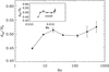 |
Fig. 9. Overshooting depth normalised by the pressure scale height at zCZ as a function of Re for Set R. The inset shows dos/HP as a function of Ma = urms/(gd)1/2. |
The current results suggest that overshooting is roughly constant as a function of Re. We note, however, that the data points with the highest values of Re (Runs R6 and R7) in Fig. 9 could not be run sufficiently long to establish that they are truly in a statistically stationary state. Thus the values of dos from these runs should be considered as upper limits. In any case, these results are at odds with those obtained by Hotta (2017), who found a steeply declining trend as a function of Re. This, however, is likely because Hotta (2017) modified the heat conductivity in the radiative layer to speed up thermal relaxation (see Sect. 4.5), and possibly exacerbated by the varying effective Prandtl number in his models (Sect. 4.2).
The inset of Fig. 9 shows dos/Hp as a function of Ma which quantifies the overall magnitude of the convective velocity. The current data suggest that the overshooting depth is independent of the overall velocity. This is at odds with Zahn (1991), for instance, who derived a Ma3/2 dependence. However, the range of values explored here is too narrow to draw definite conclusions.
4.4. Transition from the nearly adiabatic to the radiative zone
The superadiabatic temperature gradient from the runs in Set K is shown in Fig. 10. The value of ∇ − ∇ad in the RZ is close to that of the hydrostatic solution with ∇T = const. in a polytropic atmosphere with adiabatic index n = 13/4, that is,  =−17/85 ≈ −0.165 (see also Käpylä et al. 2019a). The transition from nearly adiabatic to the radiative gradient becomes increasingly sharper as ℱn decreases (e.g. Käpylä et al. 2007). Furthermore, the temperature gradient in the upper part of the OZ also approaches adiabatic as a function of ℱn, suggesting penetration in the nomenclature of Zahn (1991).
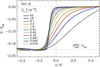 |
Fig. 10. Superadiabatic temperature gradient at the bottom of the CZ in Set K. The normalised energy flux in each run is indicated in the legend. The vertical dotted line indicates the position of the bottom of the CZ in the initial state, and |

The CZ is characterised by ∇ ≈ ∇ad, whereas in the radiative zone,  . Thus a rough estimate of the width of the transition between the zones and its dependence on ℱn is obtained by computing the vertical derivative of ∇ − ∇ad, taking its maximum, and computing where the derivative drops below a fixed fraction of the maximum. Here the threshold was set at half the maximum value. The results for the computed depth of the transition δtrans from Set K are shown as a function of ℱn in Fig. 11. The results indicate a power-law
  for ℱn ≲ 10−4. For higher values of ℱn the approximation ∇ ≈ ∇ad is no longer accurate in the CZ and the results deviate from the general trend. Extrapolating from δtrans ≈ 0.1Hp for ℱn = 1.9 × 10⁻⁷, a value of δtrans ≈ 7.9 × 10⁻³Hp is obtained for the solar value of ℱn ≈ 4 × 10⁻¹¹. This corresponds to roughly 400 km and indicates a sharp transition between overshoot and radiative zones. This is similar to what Schmitt et al. (1984) found based on a non-local ML model.
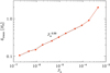 |
Fig. 11. Depth of the transition δtrans from nearly adiabatic to radiative zones as a function of input flux ℱn normalised by the pressure scale height at zCZ from Set K. |
4.5. Modified heat conductivity in the radiative zone
The study of Hotta (2017) reached the lowest value of ℱn in the literature thus far, with ℱn = 5 × 10⁻⁷. However, these results were obtained by modifying the heat conductivity in the radiative and overshoot layers while the simulations were running. This was done to achieve a statistically stationary state without having to run a full thermal diffusion time. This procedure is sometimes used in anelastic simulations in order to avoid having to run a prohibitively long Kelvin–Helmholtz time (e.g. Brun et al. 2011, 2017). While this procedure can potentially shorten the time to saturation considerably, it can have serious repercussions for overshooting. To demonstrate this, a new run was branched off from Run S7 in which the profile of  in the OZ and RZ was modified. The procedure entails computing the energy flux from the non-relaxed run and modifying
  such that the sum of all the fluxes matches Ftot in the RZ and OZ (Hotta 2017), that is,
 (36)
(36)
The original and modified profiles of  for Runs S7 and S7m are shown in Fig. 12. It is important to note that this procedure alters a crucial system parameter of the model and that the modification can be applied at an arbitrary time in the non-relaxed phase of the simulation.
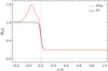 |
Fig. 12. Profiles of K, normalised by Kbot, from Runs S7 (black) and S7m (red). The bottom of the initially unstable layer is indicated by the vertical dotted line at z = 0. |
What happens in practice is that in the early phases of the simulations the cooling at the surface, in combination with weak radiative diffusion in the CZ, drives efficient convection that overshoots significantly into the radiative layer. This leads to a nearly adiabatic temperature gradient and to a reduced radiative flux in the upper part of the RZ. If ℱn is low, the radiative flux is not replenished rapidly enough and the initially vigorous convection cannot be maintained. This leads to a long period of slow evolution in which part of the heat coming from below is deposited in the RZ, OZ, and DZ such that the temperature gradient gradually steepens there to ultimately allow for the total flux to be transmitted. In the standard scenario (Run S7), the heat conductivity is fixed and the temperature gradient steepens, which means that the upper part of the RZ becomes less stiff, allowing relatively deep overshooting, see Fig. 13. The situation is exactly the opposite in Run S7m: the temperature gradient remains shallow and the stratification is significantly stiffer in comparison to the case where  was not altered.
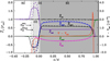 |
Fig. 13. Time-averaged total (black dash-dotted), convective (black), enthalpy (blue), radiative (dark purple), kinetic energy (light purple), and cooling (green) fluxes from Runs S7 (solid) and S7m (dashed). The vertical dotted lines indicate the bottoms of the buoyancy (BZ) and Deardorff zones (DZ). The bottom of the overshoot zone (OZ) for Run S7 (S7m) is denoted by the dashed (dot-dashed) vertical line. |
Figure 13 also shows that the modification of the heat conductivity has serious repercussions for the overshooting depth: dos is reduced by roughly 30 per cent from 0.33Hp in Run K7 to 0.23Hp in Run K7m. This result demonstrates that changing  during the run leads to a substantial underestimation of the overshooting depth. This is particularly relevant for the higher resolution cases where the modification of
  presumably has to be made at an earlier stage. This might explain the strongly decreasing overshooting depth as a function of ℱn in the study of Hotta (2017).
5. Conclusions
The scaling of convective overshooting at the base of the CZ was studied as a function of the imposed energy flux, Reynolds number, and different heat conduction profiles and prescriptions. Using heat conductivity based on Kramers opacity, or a similar smoothly varying, but fixed, profile leads to a  dependence for ℱn ≲ 10−5. Furthermore, dos is consistent with a constant as a function of the Reynolds and Péclet number in the range Re = 9…523 in cases where
  . A somewhat steeper power,
  was found in cases with a fixed step profile for the heat conduction. These results thus indicate a much milder dependence on the imposed energy flux than previous studies in the literature (Singh et al. 1998; Hotta 2017). Numerical experiments with set-ups where the SGS diffusion was turned off led to a steep power law (
 ) similar to the power laws reported earlier. Otherwise identical runs with relatively weak SGS diffusion with
  and 10, on the other hand, produced shallower dependences (
 , and
, and  , respectively). The cause for a steep power law in the case without SGS entropy diffusion is that the effective Prandtl number increases proportional to ℱn, causing the temperature fluctuations to increase. In such cases a smaller velocity fluctuation is needed to carry the same flux, which leads to reduced overshooting. This is the most likely cause for the steep power laws reported by Singh et al. (1998) and Tian et al. (2009), where the effective Prandtl number in the overshoot layer is likely much larger than unity. A similar argument can tentatively be made regarding the slope-limited diffusion used by Hotta (2017), but this should be tested with further experiments.
Furthermore, the current results indicate that modifying the heat conductivity in the layers below the CZ (e.g. Brun et al. 2017; Hotta 2017) leads to a substantial underestimation of the overshooting depth. The only way to extract reliable scaling of the overshooting depth as a function of ℱn currently is to run the simulations self-consistently to a thermally relaxed state without modifying the system parameters such as the heat conductivity. The present study also demonstrates the limits of this approach in that the runs with the lowest input flux require integration times of the order of several months even at a relatively low resolution of 2883. A more promising alternative to speeding up thermal saturation is to alter the thermodynamic quantities instead (e.g. Hurlburt et al. 1986; Anders et al. 2018). However, even this method has its limitations, and the applicability of this approach, for example, to rotating convection in spherical shells remains to be demonstrated.
The current results suggest that the overshooting depth in the Sun would be of the order of 𝒪(0.2),Hp which is somewhat higher than the canonical estimates of (0.05…0.1)Hp from helioseismology. Furthermore, the transition from overshoot to radiative zone is expected to be abrupt and occur over a depth of roughly 400 km. However, the present models lack rotation and magnetic fields, which have a significant effect on the convective flows in the deep parts of the solar CZ. Possibly the biggest caveat is the unrealistically large SGS Prandtl number we used in the current study. Set-ups where these constraints are relaxed will be explored in future publications.
This is due to  with
with  , Ck= const. and ℓ ∝ Δx const., and where Δx is the grid spacing.
Acknowledgments
The anonymous referee is acknowledged for the constructive comments on the manuscript. Axel Brandenburg is acknowledged for his insightful comments on the manuscript. The simulations were performed using the supercomputers hosted by CSC – IT Center for Science Ltd. in Espoo, Finland, who are administered by the Finnish Ministry of Education and the Gauss Center for Supercomputing for the Large-Scale computing project “Cracking the Convective Conundrum” in the Leibniz Supercomputing Centre’s SuperMUC supercomputer in Garching, Germany. This work was supported in part by the Deutsche Forschungsgemeinschaft Heisenberg programme (grant No. KA 4825/1-1) and the Academy of Finland ReSoLVE Centre of Excellence (grant No. 307411).
References
- Anders, E. H., Brown, B. P., & Oishi, J. S. 2018, Phys. Rev. Fluids, 3, 083502 [NASA ADS] [CrossRef] [Google Scholar]
- Barekat, A., & Brandenburg, A. 2014, A&A, 571, A68 [NASA ADS] [CrossRef] [EDP Sciences] [Google Scholar]
- Basu, S. 1997, MNRAS, 288, 572 [NASA ADS] [Google Scholar]
- Bekki, Y., Hotta, H., & Yokoyama, T. 2017, ApJ, 851, 74 [NASA ADS] [CrossRef] [Google Scholar]
- Brandenburg, A. 2003, in Computational Aspects of Astrophysical MHD and Turbulence, eds. A. Ferriz-Mas, & M. Núñez (London: Taylor and Francis), 269 [Google Scholar]
- Brandenburg, A. 2016, ApJ, 832, 6 [Google Scholar]
- Brandenburg, A., Chan, K. L., Nordlund, Å., & Stein, R. F. 2005, Astron. Nachr., 326, 681 [NASA ADS] [CrossRef] [Google Scholar]
- Brandenburg, A., Nordlund, A., & Stein, R. F. 2000, in Geophysical and Astrophysical Convection, eds. P. A. Fox, & R. M. Kerr (The Netherlands: Gordon and Breach Science Publishers), Contributions from a Workshop Sponsored by the Geophysical Turbulence Program at the National Center for Atmospheric Research, October 1995, 85 [Google Scholar]
- Brandenburg, A., & Subramanian, K. 2005, Phys. Rep., 417, 1 [NASA ADS] [CrossRef] [Google Scholar]
- Brown, B. P., Browning, M. K., Brun, A. S., Miesch, M. S., & Toomre, J. 2010, ApJ, 711, 424 [Google Scholar]
- Brummell, N. H., Clune, T. L., & Toomre, J. 2002, ApJ, 570, 825 [Google Scholar]
- Brun, A. S., & Browning, M. K. 2017, Liv. Rev. Sol. Phys., 14, 4 [Google Scholar]
- Brun, A. S., Miesch, M. S., & Toomre, J. 2011, ApJ, 742, 79 [NASA ADS] [CrossRef] [Google Scholar]
- Brun, A. S., Strugarek, A., Varela, J., et al. 2017, ApJ, 836, 192 [NASA ADS] [CrossRef] [Google Scholar]
- Cai, T. 2018, ApJ, 868, 12 [NASA ADS] [CrossRef] [Google Scholar]
- Canuto, V. M. 2011, A&A, 528, A76 [NASA ADS] [CrossRef] [EDP Sciences] [Google Scholar]
- Cattaneo, F., Brummell, N. H., Toomre, J., Malagoli, A., & Hurlburt, N. E. 1991, ApJ, 370, 282 [NASA ADS] [CrossRef] [Google Scholar]
- Chan, K. L., & Gigas, D. 1992, ApJ, 389, L87 [NASA ADS] [CrossRef] [Google Scholar]
- Deardorff, J. W. 1961, J. Atmosph. Sci., 18, 540 [NASA ADS] [Google Scholar]
- Deardorff, J. W. 1966, J. Atmosph. Sci., 23, 503 [Google Scholar]
- Deng, L., & Xiong, D. R. 2008, MNRAS, 386, 1979 [NASA ADS] [CrossRef] [Google Scholar]
- Deng, L., Xiong, D. R., & Chan, K. L. 2006, ApJ, 643, 426 [NASA ADS] [CrossRef] [Google Scholar]
- Dobler, W., Stix, M., & Brandenburg, A. 2006, ApJ, 638, 336 [NASA ADS] [CrossRef] [Google Scholar]
- Garaud, P., Ogilvie, G. I., Miller, N., & Stellmach, S. 2010, MNRAS, 407, 2451 [NASA ADS] [CrossRef] [Google Scholar]
- Gastine, T., Wicht, J., & Aubert, J. 2016, J. Fluid Mech., 808, 690 [NASA ADS] [CrossRef] [Google Scholar]
- Gough, D. O. 1969, J. Atmos. Sci., 26, 448 [NASA ADS] [CrossRef] [Google Scholar]
- Hotta, H. 2017, ApJ, 843, 52 [NASA ADS] [CrossRef] [Google Scholar]
- Hurlburt, N. E., Toomre, J., & Massaguer, J. M. 1986, ApJ, 311, 563 [NASA ADS] [CrossRef] [Google Scholar]
- Hurlburt, N. E., Toomre, J., Massaguer, J. M., & Zahn, J.-P. 1994, ApJ, 421, 245 [NASA ADS] [CrossRef] [Google Scholar]
- Käpylä, P. J., Korpi, M. J., & Tuominen, I. 2004, A&A, 422, 793 [NASA ADS] [CrossRef] [EDP Sciences] [Google Scholar]
- Käpylä, P. J., Korpi, M. J., Stix, M., & Tuominen, I. 2007, in Convection in Astrophysics, eds. F. Kupka, I. Roxburgh, & K. L. Chan, IAU Symp., 239, 437 [NASA ADS] [Google Scholar]
- Käpylä, P. J., Rheinhardt, M., Brandenburg, A., et al. 2017, ApJ, 845, L23 [NASA ADS] [CrossRef] [Google Scholar]
- Käpylä, P. J., Viviani, M., Käpylä, M. J., Brandenburg, A., & Spada, F. 2019a, Geophys. Astrophys. Fluid Dyn., 113, 149 [NASA ADS] [CrossRef] [Google Scholar]
- Käpylä, P. J., Gent, F. A., Olspert, N., Käpylä, M. J., & Brandenburg, A. 2019b, Geophys. Astrophys. Fluid Dyn., 113 [Google Scholar]
- Karak, B. B., Käpylä, P. J., Käpylä, M. J., et al. 2015, A&A, 576, A26 [NASA ADS] [CrossRef] [EDP Sciences] [Google Scholar]
- Karak, B. B., Miesch, M., & Bekki, Y. 2018, Phys. Fluids, 30, 046602 [NASA ADS] [CrossRef] [Google Scholar]
- Korre, L., Brummell, N., & Garaud, P. 2017, Phys. Rev. E, 96, 033104 [NASA ADS] [CrossRef] [Google Scholar]
- Korre, L., Garaud, P., & Brummell, N. H. 2019, MNRAS, 484, 1220 [NASA ADS] [CrossRef] [Google Scholar]
- Krause, F., & Rädler, K.-H. 1980, Mean-field Magnetohydrodynamics and Dynamo Theory (Oxford: Pergamon Press) [Google Scholar]
- Kupka, F. 1999, ApJ, 526, L45 [NASA ADS] [CrossRef] [Google Scholar]
- Kupka, F., & Muthsam, H. J. 2017, Liv. Rev. Comp. Astrophys., 3, 1 [NASA ADS] [CrossRef] [Google Scholar]
- Moffatt, H. K. 1978, Magnetic Field Generation in Electrically Conducting Fluids (Cambridge: Cambridge University Press) [Google Scholar]
- Nelson, N. J., Featherstone, N. A., Miesch, M. S., & Toomre, J. 2018, ApJ, 859, 117 [NASA ADS] [CrossRef] [Google Scholar]
- Nordlund, A., Brandenburg, A., Jennings, R. L., et al. 1992, ApJ, 392, 647 [NASA ADS] [CrossRef] [Google Scholar]
- Ossendrijver, M. 2003, A&ARv, 11, 287 [Google Scholar]
- Pidatella, R. M., & Stix, M. 1986, A&A, 157, 338 [NASA ADS] [Google Scholar]
- Pratt, J., Baraffe, I., Goffrey, T., et al. 2017, A&A, 604, A125 [NASA ADS] [CrossRef] [EDP Sciences] [Google Scholar]
- Rempel, M. 2004, ApJ, 607, 1046 [NASA ADS] [CrossRef] [Google Scholar]
- Renzini, A. 1987, A&A, 188, 49 [NASA ADS] [Google Scholar]
- Rogers, T. M., Glatzmaier, G. A., & Jones, C. A. 2006, ApJ, 653, 765 [NASA ADS] [CrossRef] [Google Scholar]
- Roxburgh, L. W., & Simmons, J. 1993, A&A, 277, 93 [NASA ADS] [Google Scholar]
- Rüdiger, G. 1989, Differential Rotation and Stellar Convection. Sun and Solar-type Stars (Berlin: Akademie Verlag) [Google Scholar]
- Saikia, E., Singh, H. P., Chan, K. L., Roxburgh, I. W., & Srivastava, M. P. 2000, ApJ, 529, 402 [NASA ADS] [CrossRef] [Google Scholar]
- Schmitt, J. H. M. M., Rosner, R., & Bohn, H. U. 1984, ApJ, 282, 316 [NASA ADS] [CrossRef] [Google Scholar]
- Shaviv, G., & Salpeter, E. E. 1973, ApJ, 184, 191 [NASA ADS] [CrossRef] [Google Scholar]
- Singh, H. P., Roxburgh, I. W., & Chan, K. L. 1995, A&A, 295, 703 [NASA ADS] [Google Scholar]
- Singh, H. P., Roxburgh, I. W., & Chan, K. L. 1998, A&A, 340, 178 [NASA ADS] [Google Scholar]
- Skaley, D., & Stix, M. 1991, A&A, 241, 227 [NASA ADS] [Google Scholar]
- Snellman, J. E., Käpylä, P. J., Käpylä, M. J., Rheinhardt, M., & Dintrans, B. 2015, Astron. Nachr., 336, 32 [NASA ADS] [CrossRef] [Google Scholar]
- Stein, R. F., & Nordlund, A. 1989, ApJ, 342, L95 [NASA ADS] [CrossRef] [PubMed] [Google Scholar]
- Stein, R. F., & Nordlund, Å. 1998, ApJ, 499, 914 [Google Scholar]
- Stix, M. 2002, The Sun: An Introduction (Berlin: Springer) [Google Scholar]
- Tian, C.-L., Deng, L.-C., & Chan, K.-L. 2009, MNRAS, 398, 1011 [NASA ADS] [CrossRef] [Google Scholar]
- Tremblay, P.-E., Ludwig, H.-G., Freytag, B., et al. 2015, ApJ, 799, 142 [Google Scholar]
- van Ballegooijen, A. A. 1982, A&A, 113, 99 [NASA ADS] [Google Scholar]
- Vitense, E. 1953, Z. Astrophys., 32, 135 [NASA ADS] [Google Scholar]
- Weiss, A., Hillebrandt, W., Thomas, H.-C., & Ritter, H. 2004, Cox and Giuli’s Principles of Stellar Structure (Cambridge, UK: Cambridge Scientific Publishers Ltd) [Google Scholar]
- Xiong, D. R. 1985, A&A, 150, 133 [NASA ADS] [Google Scholar]
- Yadav, R. K., Gastine, T., Christensen, U. R., Duarte, L. D. V., & Reiners, A. 2016, Geophys. J. Int., 204, 1120 [NASA ADS] [CrossRef] [Google Scholar]
- Zahn, J.-P. 1991, A&A, 252, 179 [NASA ADS] [Google Scholar]
- Zhang, C., Deng, L., Xiong, D., & Christensen-Dalsgaard, J. 2012, ApJ, 759, L14 [NASA ADS] [CrossRef] [Google Scholar]
- Zhang, Q. S. 2013, ApJS, 205, 18 [NASA ADS] [CrossRef] [Google Scholar]
- Ziegler, U., & Rüdiger, G. 2003, A&A, 401, 433 [NASA ADS] [CrossRef] [EDP Sciences] [Google Scholar]
All Tables
All Figures
|
Fig. 1. Normalised vertical velocity |
| In the text | |
|
Fig. 2. Horizontally averaged and normalised heat conductivity |
| In the text | |
|
Fig. 3. Rayleigh numbers RaSGS (black) and RaRad (red) as functions of ℱn from Set Kh. The purple (magenta) line shows RaRad (RaSGS) from Set DS (DSS). The dotted lines show scalings expected from ML arguments. |
| In the text | |
|
Fig. 4. Normalised rms velocity |
| In the text | |
|
Fig. 5. Panels a, c, and e: total (black dash-dotted lines), convective (black), enthalpy (blue), kinetic energy (light purple), radiative (dark purple), and cooling (green) fluxes and the superadiabatic temperature gradient (red) from Runs K4, S4, and DS5, respectively. Panels b, d, and f: total averaged vertical forces (solid lines) and the power of the forces (dashed) on the upflows (red) and downflows (blue) from the same runs. The dotted lines in these panels show the corresponding viscous force and its power. The shaded areas indicate the BZ (darkest), DZ, and OZ (lightest) and the thick black line at the horizontal axis denotes the MZ. |
| In the text | |
|
Fig. 6. Panel a: vertical (z) coordinates of the bottom of the CZ (zCZ, solid lines) and OZ (zOZ, dashed). The dotted red line indicates the bottom of the domain. Panel b: overshooting depth dos normalised by the pressure scale height Hp as a function of ℱn for Sets K (black), Kh (grey), P (blue), S (red), Sh (green), DS (purple), DSS1 (cyan), and DSS2 (orange). The purple diamond denotes Run DS5h. The dotted lines show approximate power laws from fits to simulation data; see Table 5. Panel c: comparison of Sets DS, DSS1, and DSS2 with the studies of Singh et al. (1998) (red) and Tian et al. (2009) (blue). |
| In the text | |
|
Fig. 7. Effective Péclet (panel a) and Prandtl (panel b) numbers at the base of the OZ. The vertical dotted line shows the approximate position of the break in the power laws in the overshooting depth in Fig. 6b. |
| In the text | |
|
Fig. 8. Ratio of the rms vertical velocity and sound speed fluctuations from the runs in Set DS (panel a) and the runs in Set DSS (panel b). |
| In the text | |
|
Fig. 9. Overshooting depth normalised by the pressure scale height at zCZ as a function of Re for Set R. The inset shows dos/HP as a function of Ma = urms/(gd)1/2. |
| In the text | |
|
Fig. 10. Superadiabatic temperature gradient at the bottom of the CZ in Set K. The normalised energy flux in each run is indicated in the legend. The vertical dotted line indicates the position of the bottom of the CZ in the initial state, and |
| In the text | |
|
Fig. 11. Depth of the transition δtrans from nearly adiabatic to radiative zones as a function of input flux ℱn normalised by the pressure scale height at zCZ from Set K. |
| In the text | |
|
Fig. 12. Profiles of K, normalised by Kbot, from Runs S7 (black) and S7m (red). The bottom of the initially unstable layer is indicated by the vertical dotted line at z = 0. |
| In the text | |
|
Fig. 13. Time-averaged total (black dash-dotted), convective (black), enthalpy (blue), radiative (dark purple), kinetic energy (light purple), and cooling (green) fluxes from Runs S7 (solid) and S7m (dashed). The vertical dotted lines indicate the bottoms of the buoyancy (BZ) and Deardorff zones (DZ). The bottom of the overshoot zone (OZ) for Run S7 (S7m) is denoted by the dashed (dot-dashed) vertical line. |
| In the text | |
Current usage metrics show cumulative count of Article Views (full-text article views including HTML views, PDF and ePub downloads, according to the available data) and Abstracts Views on Vision4Press platform.
Data correspond to usage on the plateform after 2015. The current usage metrics is available 48-96 hours after online publication and is updated daily on week days.
Initial download of the metrics may take a while.