| Issue |
A&A
Volume 630, October 2019
|
|
|---|---|---|
| Article Number | A115 | |
| Number of page(s) | 12 | |
| Section | Astrophysical processes | |
| DOI | https://doi.org/10.1051/0004-6361/201935939 | |
| Published online | 01 October 2019 | |
Glitch time series and size distributions in eight prolific pulsars
1
Instituto de Astrofísica, Pontificia Universidad Católica de Chile, Av. Vicuña Mackenna 4860, 7820436 Macul, Santiago, Chile
e-mail: This email address is being protected from spambots. You need JavaScript enabled to view it.
2
Departamento de Física, Universidad de Santiago de Chile, Avenida Ecuador 3493, 9170124 Estación Central, Santiago, Chile
3
Department of Physics and McGill Space Institute, McGill University, 3600 Rue University, H3A 2T8 Montreal, QC, Canada
Received:
23
May
2019
Accepted:
27
August
2019
Abstract
Context. Glitches are rare spin-up events that punctuate the smooth slow-down of the rotation of pulsars. For the Vela pulsar and PSR J0537−6910, their large glitch sizes and the times between consecutive events have clear preferred scales (Gaussian distributions), contrary to the handful of other pulsars with enough glitches for such a study. Moreover, PSR J0537−6910 is the only pulsar that shows a strong positive correlation between the size of each glitch and the waiting time until the following one.
Aims. We attempt to understand this behaviour through a detailed study of the distributions and correlations of glitch properties for the eight pulsars with at least ten detected glitches.
Methods. We modelled the distributions of glitch sizes and of the times between consecutive glitches for the eight pulsars with at least ten detected events. We also looked for possible correlations between these parameters and used Monte Carlo simulations to explore two hypotheses that could explain why the correlation so clearly seen in PSR J0537−6910 is absent in other pulsars.
Results. We confirm the above results for Vela and PSR J0537−6910, and verify that the latter is the only pulsar with a strong correlation between glitch size and waiting time to the following glitch. For the remaining six pulsars, the waiting time distributions are best fitted by exponentials, and the size distributions are best fitted by either power laws, exponentials, or log-normal functions. Some pulsars in the sample yield significant Pearson and Spearman coefficients (rp and rs) for the aforementioned correlation, confirming previous results. Moreover, for all except the Crab pulsar, both coefficients are positive. For each coefficient taken separately, the probability of this happening is 1/16. Our simulations show that the weaker correlations in pulsars other than PSR J0537−6910 cannot be due to missing glitches that are too small to be detected. We also tested the hypothesis that each pulsar may have two kinds of glitches, namely large, correlated ones and small, uncorrelated ones. The best results are obtained for the Vela pulsar, which exhibits a correlation with rp = 0.68 (p-value = 0.003) if its two smallest glitches are removed. The other pulsars are harder to accommodate under this hypothesis, but their glitches are not consistent with a pure uncorrelated population either. We also find that all pulsars in our sample, except the Crab pulsar, are consistent with the previously found constant ratio between glitch activity and spin-down rate, ν̇g/|ν̇| = 0.010±0.001, even though some of them have not shown any large glitches.
Conclusions. To explain these results, we speculate except in the case of the Crab pulsar, that all glitches draw their angular momentum from a common reservoir (presumably a neutron superfluid component containing ≈1% of the star’s moment of inertia). However, two different trigger mechanisms could be active, a more deterministic one for larger glitches and a more random one for smaller ones.
Key words: methods: data analysis / stars: neutron / stars: rotation / pulsars: general / pulsars: individual: PSR J0537−6910
© ESO 2019
1. Introduction
The rotation frequencies, ν, of pulsars generally decrease slowly in time, but they occasionally experience sudden increases, Δν, that are usually accompanied by increases in the absolute value of their spin-down rates,  (Radhakrishnan & Manchester 1969; Reichley & Downs 1969; Shemar & Lyne 1996). These spin-up events, known as glitches, are infrequent, not periodic, and cover a wide range of sizes (from Δν/ν ∼ 10−11 to Δν/ν ∼ 10−5; Espinoza et al. 2011; Yu et al. 2013). The mechanism that generates these events is not completely understood, but they are believed to be caused by angular momentum transfer from an internal neutron superfluid to the rest of the neutron star (Anderson & Itoh 1975).
Thanks to the few long-term monitoring campaigns continue to operate, some since the 1970s (e.g. Hobbs et al. 2004; Yu et al. 2013), the number of detected glitches has slowly increased, thereby improving the significance of statistical studies in pulsar populations. McKenna & Lyne (1990), Lyne et al. (2000), and Espinoza et al. (2011) showed that the glitch activity  (defined as the mean frequency increment per unit of time due to glitches) correlates linearly with
  . They also found that young pulsars (using the characteristic age,
  , as a proxy for age), which also have the highest
  , exhibit glitches more often than older pulsars with rates that vary from about one glitch per year to one per decade among the young pulsars. Using a larger and unbiased sample, Fuentes et al. (2017) confirmed that the size distribution of all glitches in a large and representative sample of pulsars is multi-modal (recently also seen by Konar & Arjunwadkar 2014; Ashton et al. 2017) with at least two well-defined classes of glitches: large glitches in a relatively narrow range Δν ∼ (10−30) μHz, and small glitches with a much wider distribution, from ∼10 μHz down to at least 10−4 μHz. Furthermore, Fuentes et al. (2017) found that a constant ratio,
  , is consistent with the behaviour of nearly all rotation-powered pulsars and magnetars. The only exception are the few very young pulsars, which have the highest spin-down rates, such as the Crab pulsar (PSR B0531+21) and PSR B0540−69.
Because glitches are rare events, the number of known glitches in the vast majority of pulsars is not substantial enough to perform robust statistical analyses on individual bases. This has made people focus on the few objects that have the largest numbers of detected glitches (about ten pulsars). The statistical distributions of glitch sizes and times between consecutive glitches (waiting times), for the nine pulsars with more than five known glitches at the time, were studied by Melatos et al. (2008). They found that seven out of the nine pulsars exhibited power-law-like size distributions and exponential waiting time distributions. The distributions of the other two (PSRs J0537−6910 and B0833−45, the Vela pulsar) were better described by Gaussian functions, which set preferred sizes and time scales. These results have been further confirmed by Fulgenzi et al. (2017) and Howitt et al. (2018), who also found that there are at least two main behaviours among the glitching pulsars.
Correlations between glitch sizes and the times to the nearest glitches, either backwards or forwards, are naturally expected. We know that glitch activity is driven by the spin-down rate (Fuentes et al. 2017), which suggests that glitches are the release of some stress that builds up at a rate determined by  . If the stress is completely released at each glitch, then one should expect a correlation between size and the time since the last glitch. Conversely, if glitches occur when a certain critical state is reached, one should expect a correlation between size and the time to the next glitch, as longer times would be needed to come back to the critical state after the largest glitches. Moreover, if both assumptions are indeed correct, glitches would all be of equal sizes and occur periodically. However, with the exception of PSR J0537−6910 (see below), no other pulsars have shown significant correlations between glitch sizes and the times to the nearest events (e.g. Wang et al. 2000; Yuan et al. 2010; Melatos et al. 2018). This may be partly due to small-number statistics and might improve in the future, provided a substantial number of pulsars continue to be monitored for glitches.
The case of PSR J0537−6910, however, is very clear. With more than 40 glitches detected in ∼13 yr, the statistical conclusions about its behaviour are much more significant than for any other pulsar. As first reported by Middleditch et al. (2006), its glitch sizes exhibit a strong correlation with the waiting time to the following glitch (see also Antonopoulou et al. 2018; Ferdman et al. 2018, who confirmed the correlation using twice as much data).
Antonopoulou et al. (2018) interpret this behaviour as an indication that glitches in this pulsar occur only once some threshold is reached. Moreover, this behaviour would imply that not necessarily all the stress is released in the glitches, thereby giving rise to the variety of (unpredictable) glitch sizes observed and the lack of backwards time correlation.
In this work we study the sequence of glitches in the pulsars with at least ten detected events, by characterizing their distributions of glitch sizes and waiting times between successive glitches. Also, we test two hypotheses to explain why most pulsars do not show a correlation between glitch size and time to the following glitch: the effects of undetected small glitches and the possibility that two different classes of glitches are present in each pulsar.
2. Pulsars with at least ten detected glitches
To date, there are eight pulsars with at least 10 detected glitches (Fig. 1). PSRs J0205+6449, B0531+21 (the Crab pulsar), B1737−30, B1758−23, and J0631+1036 have been observed regularly by the Jodrell Bank Observatory (JBO, Hobbs et al. 2004). PSR B1338−62 has been observed by the Parkes telescope, and the Vela pulsar has been observed by several telescopes, including Parkes, the Jet Propulsion Laboratory, and others in Australia and South Africa (e.g. Downs 1981; McCulloch et al. 1987; Yu et al. 2013; Buchner 2013). PSR J0537−6910 is the only object in our sample not detected in the radio band and was observed for 13 years by the Rossi X-ray Timing Explorer (RXTE; Antonopoulou et al. 2018; Ferdman et al. 2018). Glitch epochs and sizes were taken from the JBO online glitch catalogue1, where more information and the appropriate references for each measurement can be found.
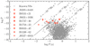 |
Fig. 1. Upper part of the P−Ṗ diagram for all known pulsars. The pulsars in our sample have at least ten detected glitches and are labelled with different symbols. Lines of constant spin-down rate |

Figures 2 and 3 show that the Vela pulsar and PSR J0537−6910 produce glitches of similar sizes, particularly large glitches (Δν > 10 μHz), and in fairly regular time intervals. The absence of smaller glitches in these pulsars is not a selection effect, as it is quite unlikely that a considerable amount of glitches with sizes up to Δν ∼ 10 μHz, far above the detection limits reported in the literature (see Watts et al. 2015, and text below), could have gone undetected. On the other hand, the rest of the pulsars exhibit irregular waiting times and cover a wider range of sizes (Δν ∼ 10−3 − 10 μHz).
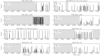 |
Fig. 2. Logarithm (base 10) of glitch sizes Δν (with Δν measured in μHz) as a function of the glitch epoch for the pulsars in the sample. The grey areas mark periods of time in which there were no observations for more than 3 months. Ng is the number of glitches detected in the respective pulsar, until 20 April 2019 (MJD 58593). To build a continuous sample, in the analyses of the Crab pulsar, we only use the 25 glitches after MJD 45000, when daily observations started (Espinoza et al. 2014). All panels share the same scale, in both axes. |
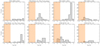 |
Fig. 3. Distribution of logΔν (with Δν measured in μHz) for the pulsars in our sample. The orange areas indicate that glitches with Δν < 0.01 μHz could be missing due to detectability issues. |
The cadence of the timing observations varies considerably from pulsar to pulsar (and even with time for individual pulsars), and the sensitivity of the observations, from which the glitch measurements were performed, are also different between different pulsars. This means that the chances of detecting very small glitches are different for each pulsar and that the completeness of the samples towards small events might also be different (Espinoza et al. 2014). Nonetheless, in this study we use a single value to represent the glitch size below which samples are likely to be incomplete due to detectability issues. For an observing cadence of 30 days and a rotational noise of 0.01 rotational phases, glitch detection is severely compromised below sizes Δν ∼ 10−2 μHz, especially if their frequency derivative steps are larger than  (see Watts et al. 2015). We use the above numbers to characterize the glitch detection capabilities in this sample of pulsars, but we note that such cadence and rotational noise are rather pessimistic values in some cases.
3. Distributions of glitch sizes and times between glitches
In the following, we model the distributions of glitch sizes (Δν, measured in μHz) and the distributions of times between successive glitches (Δτ, measured in yr) for each pulsar in our sample. Four probability density distributions are considered: Gaussian,
![Mathematical equation: $$ \begin{aligned} M(x|\mu ,\sigma ) = C_{\rm Gauss}\,\exp \left[\frac{-(x-\mu )^2}{2\sigma ^2}\right]{,} \end{aligned} $$](/articles/aa/full_html/2019/10/aa35939-19/aa35939-19-eq11.gif) (1)
(1)
power-law,
 (2)
(2)
log-normal,
![Mathematical equation: $$ \begin{aligned} M(x|\mu _{\text{ L-N}},\sigma _{\text{ L-N}}) = \dfrac{C_{\text{ L-N}}}{x}\,\exp \left[\frac{-(\ln x-\mu _{\text{ L-N}})^2}{2\sigma _{\text{ L-N}}^2}\right], \end{aligned} $$](/articles/aa/full_html/2019/10/aa35939-19/aa35939-19-eq13.gif) (3)
(3)
and exponential,
![Mathematical equation: $$ \begin{aligned} M(x|\lambda ) = \lambda \, \exp \left[-\lambda (x-x_{\rm {min}})\right]. \end{aligned} $$](/articles/aa/full_html/2019/10/aa35939-19/aa35939-19-eq14.gif) (4)
(4)
The set {μ, σ, α, μL-N, σL-N, λ} are the fitting parameters. All the distributions are normalized in the range xmin to ∞. Formally, xmin is given by detection limits. However, it is not simple to define precise values for Δνmin and Δτmin for each pulsar. Thus we use Δνmin = 10−2 μHz for the glitch sizes (see previous section), and the smallest interval of time between glitches in each pulsar as Δτmin.
For the Gaussian and log-normal distributions the normalization constants CGauss and CL-N were found numerically. We use the maximum likelihood technique to obtain the parameters of the models that describe best the data, and use the Akaike Information Criterion (AIC; Akaike 1974) to compare the different models (see also the appendix in Fuentes et al. 2017).
Figures 4 and 5 and Tables 1 and 2 summarize the results of fitting these distributions to each pulsar. There is no single distribution type that can simultaneously describe all the pulsars satisfactorily, for either sizes or waiting times. The size distributions present a large variety (as also found in the model of Carlin & Melatos 2019): the log-normal distribution gives the best fit for the Crab pulsar and PSR B1338−62, power-law for PSRs J0631+1036, B1737−30, and J0205+6449, and exponential for PSRs B1758−23.
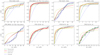 |
Fig. 4. Cumulative distribution of glitch sizes and model fits. The best-fitting models are indicated by thicker curves. |
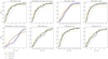 |
Fig. 5. Cumulative distribution of waiting times between successive glitches and model fits. The best-fitting models are indicated by thicker curves. |
Distributions of glitch sizes: results of fits and AIC weights for each model; using glitches with Δν ≥ 0.01 μHz.
Distributions of waiting times between successive glitches: results of fits and AIC weights for each model.
We also note that PSR J0205+6449 and PSR B1758−23 are the pulsars with the fewest recorded glitches in the sample (both have 13 glitches detected), hence we ought to wait and confirm this result once more events are detected.
In the case of PSRs J0537−6910 and B0833−45 (Vela), the best fit for both size and waiting time distributions are Gaussian functions. Their size distributions are centred at large sizes Δν ≈ 15 and 20 μHz, respectively, consistent with the peak of large glitches in the combined distribution for all pulsars (Fuentes et al. 2017).
The distributions of times between successive glitches offer more homogeneous results. Besides the case of PSR J0537−6910 and the Vela pulsar (best modelled by Gaussian functions), the waiting time distributions for all the other pulsars are best represented by exponential functions. These results are in agreement with Melatos et al. (2008), Wang et al. (2012), and Howitt et al. (2018) for almost all the pulsars studied. The only exception is PSR B1338−62, for which Howitt et al. (2018) reported a local maximum in the distribution and classified this pulsar as a quasi-periodic glitcher.
If Δνmin is set to the size of the smallest detected glitch in each pulsar (rather than to 10−2 μHz), the results of the fits are very similar, and give parameters within the uncertainties presented in Table 1.
4. Time series correlations: Glitch size and time to the next glitch
Different studies have shown that for PSR J0537−6910 the glitch magnitudes Δνk are strongly correlated with the waiting times to the following glitch Δτk + 1 (Middleditch et al. 2006; Antonopoulou et al. 2018; Ferdman et al. 2018, and see Fig. 6). Recently, Melatos et al. (2018), tested whether this correlation is also present in the rest of the pulsars with at least 10 glitches detected, and found that, in addition to PSR J0537−6910, PSR B1758−23 also exhibits a significant correlation between glitch sizes and waiting times until the next glitch.
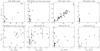 |
Fig. 6. Time to next glitch, Δτk + 1, as a function of glitch size, Δνk, for all the pulsars in the sample. |
In the following, we analyse the presence of this correlation in our sample of pulsars. Data are plotted in Fig. 6 and correlation coefficients are listed in Table 3. Our results are consistent with Melatos et al. (2018), with minor differences since the glitch samples are not exactly the same, and we have the additional source PSR J0205+6449.
Correlation coefficients between Δνk and Δτk + 1.
Clearly, none of the other pulsars exhibits a correlation as clear as PSR J0537−6910. However, for PSRs J0205+6449, J0631+1036, B1338−62, and B1758−23, the Pearson correlation coefficients are larger than 0.5 and the p-values are ≲10−3. Therefore, at 95% confidence level (p-values < 0.05), we can reject the null hypothesis that Δνk and Δτk + 1 are uncorrelated in these pulsars. Since the Pearson coefficient can be dominated by outliers, we also compute the Spearman rank correlation coefficient, obtaining similar or even stronger correlations, except for PSR J0631+1036.
It is also interesting to note that not only for PSR J0537−6910, but for all pulsars in the sample except the Crab, both the Pearson and Spearman correlation coefficients are positive. The probability of finding at least six out of seven pulsars having the same sign as our reference case, just by chance, is rather low. The probability of getting exactly k successes among n trials, with 1/2 success probability in each trial, is  . Thus, the probability of getting at least six successes in seven trials is
 (5)
(5)
This low probability suggests that the waiting time to the following glitch is at least partially regulated by the size of the previous glitch.
In order to explain why the correlation for all other pulsars is much less clear than for PSR J0537−6910, we explore two hypotheses, both of which are motivated by noting that most glitches in PSR J0537−6910 are large.
The first hypothesis is that the correlation is intrinsically present in the full population of glitches of each pulsar, but glitches below a certain size threshold are not detected, thereby increasing by random amounts the times between the detected ones and worsening the correlation.
The second hypothesis is that there are two classes of glitches: glitches above a certain threshold size that follow the correlation, and glitches below the same threshold that are uncorrelated.
4.1. Hypothesis I: Incompleteness of the sample
In order to test the first hypothesis, we simulate a hypothetical pulsar with 100 glitches that follow a perfect correlation between Δνk and Δτk + 1. The events smaller than a certain value are then removed to understand the effect of their absence in the correlation. The procedure is the following:
Firstly, glitch sizes are generated from a power-law distribution given by dN/dΔν ∝ Δν−α, with power-law index α > 1. We choose a power-law distribution because it mainly produces small events, and we want to see the effect of removing a substantial fraction of them. Several different choices for α were considered. Here we only show the results for α = 1.2 and 1.4, as they generate distributions that resemble some of the ones observed. The distributions do not have an upper cutoff, and the lower limit was varied so that, after reducing the sample of glitches (as we explain in step 3 below), the resulting sample covers the typical observed range of glitch sizes (10−2 − 102 μHz).
Secondly, the time to the next glitch Δτk + 1 is computed in terms of the glitch size Δνk as:
 (6)
(6)
The value of the proportionality constant C is irrelevant in this case, since we are simulating a generic pulsar.
Thirdly, the previous steps are repeated until a sequence of 100 glitches is reached. Then the 80 smallest are removed, thereby leaving a reduced sample of 20 to be analysed, which is comparable to the number of glitches observed in each of our 8 pulsars. The lower limit for the distribution is computed analytically so that, after reducing the sample of glitches, the final sample covers the typical observed range of glitch sizes (10−2 − 102 μHz).
Finally, we calculate the time interval between each pair of successive glitches in the reduced sample, and determine both the Spearman and Pearson correlation coefficients between Δνk and Δτk + 1.
After simulating 104 cases, it was found that removing all glitches smaller than a certain value has a minor effect on the correlation. Representative realizations are shown in Fig. 7, where the correlation between Δνk and Δτk + 1 is plotted in log-scale to show more clearly the dispersion produced by the removal of the smallest glitches. We observe that missing small glitches does not substantially worsen the correlation: more than 90% of the realizations give correlation coefficients ≥0.95 (both Pearson and Spearman).
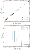 |
Fig. 7. Reduced samples of simulated glitches from an assumed parent distribution dN/dΔν ∝ Δν−α with a perfect correlation Δτk + 1 = CΔνk, with C = 0.21 yr μHz−1. Top: resulting correlation between Δνk and Δτk + 1. Bottom: corresponding distributions of logΔν for the reduced samples of glitches. For both panels, each colour (and point marker) represents a typical realization in the simulations, for different power-law exponents as shown in the legends. |
For α > 1.4 the distribution becomes narrower, accumulating towards the lower limit. Since a large fraction of the simulated glitches have very similar sizes, after removing the 80 smallest glitches the correlation does worsen, and yields correlation coefficients between 0.4 and 0.9, which are similar to those exhibited by the real data. However, in these cases the distributions of glitch sizes differ strongly from those observed for the pulsars in our sample.
From these simulations, we conclude that it is unlikely that the non-detection of all the glitches below a certain detection limit is the explanation for the low observed correlations in pulsars other than PSR J0537−6910.
4.2. Hypothesis II: Two classes of intrinsically different glitches
The second hypothesis states that pulsars exhibit two classes of glitches: larger events, which follow a linear correlation between Δνk and Δτk + 1; and smaller events, for which these variables are uncorrelated. We allow the point of separation between large and small glitches to be different for each pulsar.
To visualize whether this hypothesis works, correlation coefficients (for the same pair of variables, Δνk and Δτk + 1) were calculated for sub-sets of glitches of the original sample. The sub-sets are defined as all glitches with sizes larger or equal to a given Δνmin. Correlation coefficients as a function of Δνmin are plotted in Fig. 8 for each pulsar. Visual inspection of the plots immediately tells us that by removing small glitches no pulsar reaches the level of correlation observed for PSR J0537−6910, for both correlation tests.
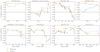 |
Fig. 8. Pearson (orange squares) and Spearman (blue dots) correlation coefficients for glitches larger or equal than Δνmin. Each panel represents a pulsar in our sample. For each pulsar, the last point in the plot was calculated with its five largest glitches. Some pulsars are shown in log-scale for a better visualization. |
In the following we explore the curves in Fig. 8 in some more detail. For that purpose, Monte Carlo simulations of pulsars with correlated and uncorrelated glitches were performed. Since the underlying glitch size distributions of the pulsars in the sample are unknown, we use the measured values of a given pulsar. The following is the procedure for one realization:
Firstly, the glitches larger than a certain value Δν⋆ are chosen in random order and assigned epochs according to their size. The first one is set at an arbitrary epoch and the epochs of the following ones are assigned according to
 (7)
(7)
where x is drawn from a Gaussian distribution centred at  and with a standard deviation equal to
  . The latter allows us to introduce a dispersion in the correlation of the simulated glitches.
The distribution of log(Δτk + 1/Δνk) for all glitches with Δν > 5 μHz in PSR J0537−6910 can be well modelled by a Gaussian distribution with standard deviation σ0537 = 0.085 (in logarithmic scale, if Δτk + 1 is measured in days and Δνk is measured in μHz).
In the simulations,  was set either to zero (i.e. x = log(C), perfect correlation) or to multiples of σ0537.
Secondly, the glitches smaller than Δν⋆ are distributed randomly over the time span between the first and the last correlated glitches. The resulting waiting times of all, correlated and uncorrelated glitches are then multiplied by a factor that ensures that their sum equals the time in between the first and the last observed glitches.
Finally, the previous steps were repeated 104 times for each considered value of Δν⋆.
The plots in Fig. 9 show the results of simulations using the glitch sizes of PSR J0537−6910 and  for three values of Δν⋆. The results are shown via curves of r vs. Δνmin, to compare with Fig. 8. The shaded areas represent the 70% of the correlation coefficients closer to the median of all realizations. We visually inspected the distributions of rp and rs for all possible Δνmin values, and for many Δν⋆ cases. It was verified that the median is sufficiently close to the maximum of the distribution in most cases. Though, this tends to fail for the largest Δνmin values, where the rp and rs distributions are rather flat. But this is irrelevant because any conclusion pointing to a case in which only a few glitches are correlated (large Δνmin) would have little statistical value, regardless of the above. Thus we are confident that the shaded areas effectively cover the most possible outcomes of series of glitches under the assumptions considered.
We now use the plots in Fig. 9 to understand the curves of the correlation coefficients as functions of Δνmin in Fig. 8, in the frame of Hypothesis II
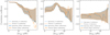 |
Fig. 9. Correlation coefficients rp (orange) and rs (blue) vs. Δνmin for simulated glitches under hypothesis II, and for three Δν⋆ cases: left: when all glitches are correlated (Δν⋆ ∼ 0); middle: about half of them are correlated (Δν⋆ = 12.39 μHz); right: none of them is correlated (Δν⋆ = 40 μHz). Shaded regions represent the values of the 70% closer to the median of all realizations. The dashed lines show particular realizations. These simulations used the glitch sizes of PSR J0537−6910 and |

If all glitches were correlated, which is the case shown in the leftmost plot in Fig. 9, the correlation coefficients would decrease gradually as Δνmin increases. This is because a progressive reduction of the sample, starting from the smallest events (i.e. increasing the remaining waiting times by small random amounts), will gradually kill the correlation. We note that the correlation coefficients of the simulated glitches start at values just below 1.0 for the smallest Δνmin, just like the observations of PSR J0537−6910. This is because  in those simulations. Only for
  the simulations would start at correlation coefficients equal to 1.0.
If only glitches above a certain size Δν⋆ were correlated, the correlation coefficients would improve as small glitches are eliminated, and the remaining sub-set approaches the one in which all glitches are correlated (as in the middle plot of Fig. 9). One would expect a maximum correlation for Δνmin ∼ Δν⋆, and a gradual decrease as Δνmin increases beyond Δν⋆.
If there were no correlated glitches, we should expect a rather flat curve of low correlation coefficients oscillating around zero (rightmost plot in Fig. 9).
The behaviours just described correspond to the general trends exhibited by the shaded areas in Fig. 9, which evolve smoothly with Δνmin. However, particular realizations show abrupt variations, of both signs, just as the observations do in Fig. 8.
Clearly, PSR J0537−6910 is best represented by case (a). Indeed, both correlation coefficients for this pulsar are maximum (and very similar) when all glitches are included and they decrease gradually as the smallest glitches are removed (Fig. 8). Nonetheless, we note that rp stays above 0.9 (and pp < 3 × 10⁻¹²) for Δνmin ≤ 7 μHz, hence it is possible that the smallest glitches are not correlated. Another indication for this possibility is that the six glitches below 5 μHz fall to the right of the distribution of log(Δτk + 1/Δνk) for all glitches, and the width of the distribution is reduced considerably (from more than 2 decades to a half decade) when they are removed. In other words, the straight line that best fits the (Δτk + 1, Δνk) points passes closer to the origin (a more physically motivated situation, Antonopoulou et al. 2018), and the data exhibit a smaller dispersion around this line, when the smallest glitches are not included.
The pulsars B1338−62, and B1758−23 may in principle also correspond to case (a). As mentioned at the beginning of Sect. 4, they present mildly significant correlations when all their glitches are considered, and both their rp and rs curves in Fig. 8 decrease as Δνmin increases. By performing simulations with Δν⋆ = 0, and for different values of  , we find that the correlation coefficients of PSR B1758−23 are within the range of 70% of the possible outcomes if
  is set to 5-6 times σ0537.
For PSR B1338−62 the situation is less clear because the amplitudes of the variations of both rp and rs for Δνmin < 1 μHz are rather high. One possible interpretation is that all glitches are correlated and the variations are due to the correlation not being perfect (i.e.  ). We find that only for
  the simulations can reproduce such behaviour and the observed values. Another possibility is that Δν⋆ ∼ 0.2 μHz, which could explain the local maxima of rp and rs around that value. The maxima and subsequent values can indeed be reproduced with lower levels of noise,
  . But for smaller values of Δνmin most realizations (> 70%) give correlation coefficients below 0.5, thus they fail at reproducing the observed 0.6−0.7 at Δνmin = 0.
It is clear that Hypothesis II does not apply to this pulsar directly, and that the observations are not consistent with a set of uncorrelated glitches either. Based on the lack of glitches with sizes equal or less than 0.1 μHz after MJD ∼ 50400 (Fig. 2), we speculate that the sample might be incomplete for glitches smaller than this size after this date2.
The pulsars J0205+6449 and J0631+1036 also exhibit significant Pearson correlations when all their glitches are considered. However, their rs curves tend to increase with Δνmin rather to decrease. As mentioned before, the Pearson test can be affected by outliers, hence the behaviour we see for rp is likely due to the very broad size and waiting times distributions and the low numbers of events towards the high ends of the distributions, which produce outlier points for both pulsars (Fig. 6). It is therefore difficult to conclude anything for PSR J0631+1036. Moreover, the observed behaviour is very hard to reproduce by the simulations, even for high levels of noise (we tried up to  ). Perhaps its largest glitches (Δν ≥ 0.1 μHz) are indeed correlated, but the statistics are too low to conclude anything.
For PSR J0205+6449, however, the Spearman coefficients rs are rather high (> 0.55 for all Δνmin) and both coefficients become similar and even higher for Δνmin > 1 μHz. It is possible that glitches above this size are correlated in this pulsar. We find that the observed rp and rs, and their evolution with Δνmin, are within the 70% of simulations with Δν⋆ = 1.3 μHz and for  . We note, however, that in this case the correlation coefficients observed for Δνmin ≤ 0.1 μHz are higher than the vast majority of the realizations. Perhaps the small glitches are also correlated and follow their own relation, though we did not simulate such scenario. We conclude that the Hypothesis II does not fully explain this pulsar, although the 8 glitches above 1 μHz appear to be well correlated indeed.
The Vela pulsar is the only pulsar in the sample that seems well represented by case (b). The highest rp = 0.68 has a probability pp = 0.003 and is obtained for Δνmin ∼ 2 μHz. Both rp and rs decline monotonically for larger Δνmin values. This behaviour suggests that glitches of sizes above ∼2 μHz might indeed be correlated, but the correlation is somewhat noisy. The observed correlation coefficients fall within the middle 70% of the realizations if  and for Δν⋆ = 2-10 μHz. The case Δν⋆ = 9.35 μHz is presented in Fig. 10. We prefer this case because simulations for Δν⋆ = 2 μHz tend to fail at reproducing the low correlation coefficients (≤0.4) observed for the smallest Δνmin.
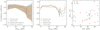 |
Fig. 10. Observations and simulations of the Vela pulsar. Left: shaded regions indicate the values obtained by the 70% closer to the median of all realizations. The observations are overlaid using dashed lines. Middle: comparison of observations (dashed) and one particular realization. Right: Δτk + 1 vs. Δνk for the same realization (red triangles) and for the observations (grey dots). Orange represents rp values and blue represents rs values in all panels. The simulations were performed using |

Finally, the cases of PSRs B0531+21 (the Crab) and B1737−30 are rather inconclusive. The Crab pulsar is perhaps the pulsar for which case (c) applies the best. Both correlation coefficients are negative or positive, and in both cases stay at relatively low absolute values, which leads to the conclusion that there are no correlated glitches in the Crab pulsar. We note that the high rp and rs values observed for Δνmin ∼ 0.6 μHz are obtained with the 5–6 largest events and that a linear fit to their Δνk − Δτk + 1 does not pass close to the origin.
The case of B1737−30 is more complex. The observations show two Δνmin values, 0.0015 and 0.03 μHz, after which the correlation coefficients decrease with the removal of more small glitches (Fig. 8). This behaviour is hard to reproduce under Hypothesis II, unless the dispersion of the correlation is increased considerably, to 10 × σ0537 or more. We conclude that Hypothesis II does not apply to this pulsar directly and that there is some extra complexity, as the data are also inconsistent with a set of purely uncorrelated glitches.
Surprisingly, even though no pulsar complies perfectly with Hypothesis II, and the only way in some cases is to increase the dispersion of the correlation ( ), there is no pulsar in the sample that is well represented by case (c) (only the Crab, to some extent).
Therefore, the sizes of at least some glitches must be positively correlated with the times to the next glitch in the available datasets. The question is why this correlation is much stronger in PSR J0537−6910 than in all other pulsars of our sample. Perhaps, this could be an effect of its particularly high spin-down rate, or the fact that most of its glitches are large. It might be also possible that the correlations are indeed there, as stated in Hypothesis II, but for some reason exhibit high  values. Maybe the fact that the glitches in PSR J0537−6910 occur so frequently ensures that the relationship stays pure. But it could also be that reality was more complex. For instance, it could be that both small and large glitches were correlated, but each of them followed a different law.
5. Other correlations
We looked for other possible correlations between the glitch sizes and the times between them. Specifically, we tried Δνk vs Δτk (size of the glitch vs. the time since the preceding glitch). For all pulsars in our sample, we did not find significant correlations for both, Pearson and Spearman (see Table 4).
Correlation coefficients for the pairs of variables (Δνk, Δτk), and (Δνk, Δνk − 1).
Melatos et al. (2018) also tested this correlation and our results are in agreement, apart from some minor differences because the glitch samples are not exactly the same
We also test Δνk vs. Δνk − 1 (size of the glitch vs. size of the previous glitch). In most cases the correlation coefficients are close to zero and the p-values are larger than 0.2 (see right panel in Table 4), that is, no individual pulsar shows a significant correlation. However, the results could still be meaningful for the sample as a whole because all the pulsars have negative correlation coefficients, except for the Spearman coefficients for PSRs J0631+1036 and B1737−30). The probability of getting all Pearson’s correlations coefficients of the same sign just by chance, regardless of whether the sign is positive or negative, is 2 × pbinom(8|8) = 0.007. This could establish an interesting constraint on the glitch mechanism: Smaller glitches are somewhat more likely to be followed by larger ones, and vice-versa. However, this statement has to be confirmed with more data in the future.
6. Glitch activity: one reservoir, two trigger mechanisms?
Fuentes et al. (2017) found that all pulsars (with the strong exception of the Crab pulsar and PSR B0540−69) are consistent with a constant ratio between the glitch activity,  , and the spin-down rate,
  , that is, ≈1% of their spin-down is recovered by the glitches. This fraction has been interpreted as the fraction of the moment of inertia in a superfluid component that transfers its angular momentum to the rest of the star in the glitches (Link et al. 1999; Andersson et al. 2012). Fuentes et al. (2017) used the observed bimodal distribution of glitch sizes to distinguish between large and small glitches, with the boundary at Δν = 10 μHz, and argued that the constant ratio is determined by the large glitches, whose rate, Ṅℓ is also proportional to
  . In this scenario, the much lower (sometimes null) glitch activities measured in many low-
 pulsars are due to their observation time spans not being long enough to include any large glitches (or any glitch at all). Interestingly, the pulsars in our sample (except the Crab) are quite consistent with the constant ratio (Fig. 11), even those, like PSRs B1338−62, B1737−30, and B1758−23, which do not have any large glitches contributing to their activities.
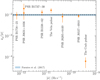 |
Fig. 11.
|


On the other hand, pulsars with higher spin-down rates also have a larger fraction of large glitches. At the highest spin-down rates ( Hz s−1), the production of large glitches becomes comparable and sometimes higher than the production of small glitches, again with the notorious exception of the Crab and PSR B0540−69. This trend is also followed by the pulsars in our sample: all large glitches (but one in PSR J0631+1036), are concentrated in PSRs J0205+6449, J0537−6910, and the Vela pulsar, which are (together with the Crab) the ones with largest
  values (see Figs. 1 and 11).
Thus, it seems to be the case that both large and small glitches draw from the same angular momentum reservoir (for all but the very young, Crab-like pulsars), but have different trigger mechanisms, the large ones being produced once a critical state is reached, whereas small ones occur in a more random fashion. For reasons still to be understood, the glitch activity of relatively younger, high  , Vela-like pulsars is dominated by large glitches, whereas for smaller
  the large glitches become less frequent, both in absolute terms and relative to the small ones (Wang et al. 2000; Espinoza et al. 2011).
In this context, it is interesting to note that recent long-term braking index measurements indicate that Vela-like pulsars move towards the region where PSRs J0631+1036, B1737−30, and B1758−23 are located on the P–Ṗ diagram (Espinoza et al. 2017).
7. Summary and conclusions
We studied the individual glitching behaviour of the eight pulsars that today have at least ten detected glitches. Our main conclusions are the following:
-
1.
We confirm the previous result by Melatos et al. (2008) and Howitt et al. (2018) that, for Vela and PSR J0537−6910, the distributions of both their glitch sizes and waiting times are best fitted by Gaussians, indicating well-defined scales for both variables. For all other pulsars studied, the waiting time distribution is best fitted by an exponential (as would be expected for mutually uncorrelated events), but they have a variety of best-fitting size distributions: a power law for PSR J0205+6449, J0631+1036, and B1737−30, a log-normal for the Crab and PSR B1338−62, and an exponential for PSR B1758−23.
-
2.
All pulsars in our sample, except for the Crab, have positive Spearman and Pearson correlation coefficients for the relation between the size of each glitch, Δνk, and the time to the following glitch, Δτk + 1 (as found by Melatos et al. 2018). For each coefficient, the probability for this happening by chance is 1/16 = 6.25%. Both coefficients also stay positive as the small glitches are removed (see Fig. 8).
-
3.
PSR J0537−6910 shows by far the strongest correlation between glitch size and waiting time until the following glitch (rp = rs = 0.95, p-values ≲10−22). Another three pulsars, PSRs J0205+6449, B1338−62, and B1758−23, have quite significant correlations (p-values ≤0.004 for both coefficients).
-
4.
Our first hypothesis to explain the much weaker correlations in all other pulsars compared to PSR J0537−6910, namely missing glitches that are too small to be detected, is very unlikely to be correct. Our Monte Carlo simulations show that, for reasonable glitch size distributions, it cannot produce an effect as large as observed.
-
5.
Our alternative hypothesis, namely that there are two classes of glitches, large correlated ones and small uncorrelated ones, comes closer to reproducing the observed relations; notably for PSRs J0205+6449 and Vela. The resulting correlations for both pulsars present dispersions that are twice the one observed for PSR J0537−6910. For the other pulsars, the required dispersion to accommodate this hypothesis are much larger.
-
6.
The correlation coefficients between the sizes of two successive glitches, Δνk − 1 and Δνk, as well as between the size of a glitch, Δνk and the waiting time since the previous glitch, Δτk, are generally not significant in individual pulsars (in agreement with Melatos et al. 2018), but they are negative for most cases, suggesting some (weaker) relation also among these variables.
-
7.
Except for the Crab, all pulsars in our sample are consistent with the constant ratio between glitch activity and spin-down rate,
 (Fuentes et al. 2017). This includes cases dominated by large glitches, as well as others with only small glitches.
 -
8.
The previous results suggest that large and small glitches draw their angular momentum from a common reservoir, although they might be triggered by different mechanisms. Large glitches, which dominate at large
 (except for the Crab and PSR B0540−69), might occur once a certain critical state is reached, while small glitches, dominating in older pulsars with lower
  , occur at essentially random times.
All the above is based on the behaviour of the pulsars with the most detected glitches. Even though we have shown before that the activity of all pulsars appears to be consistent with one single trend, these pulsars could still be outliers among the general population. Only many more years of monitoring will clarify the universality of these results.
This would be a more extreme case than those considered for the Hypothesis I because 0.1 μHz is a rather high limit.
Acknowledgments
We thank Vanessa Graber and Simon Guichandut for valuable comments on the first draft of this article. We are also grateful to Wilfredo Palma for conversations that guided us at the beginning of this work. We also thank Ben Shaw for information regarding the detection of recent glitches and for keeping the glitch catalogue up to date. This work was supported in Chile by CONICYT, through the projects ALMA31140029, Basal AFB-170002, and FONDECYT/Regular 1171421 and 1150411. J. R. F. acknowledges partial support by an NSERC Discovery Grant awarded to A. Cumming at McGill University. C. M. E. acknowledges support by the Universidad de Santiago de Chile (USACH).
References
- Akaike, H. 1974, IEEE Trans. Auto. Control, 19, 716 [Google Scholar]
- Anderson, P. W., & Itoh, N. 1975, Nature, 256, 25 [NASA ADS] [CrossRef] [Google Scholar]
- Andersson, N., Glampedakis, K., Ho, W. C. G., & Espinoza, C. M. 2012, Phys. Rev. Lett., 109, 241103 [NASA ADS] [CrossRef] [PubMed] [Google Scholar]
- Antonopoulou, D., Espinoza, C. M., Kuiper, L., & Andersson, N. 2018, MNRAS, 473, 1644 [NASA ADS] [CrossRef] [Google Scholar]
- Ashton, G., Prix, R., & Jones, D. I. 2017, Phys. Rev. D, 96, 063004 [NASA ADS] [CrossRef] [Google Scholar]
- Buchner, S. 2013, ATel, 5406 [Google Scholar]
- Carlin, J. B., & Melatos, A. 2019, MNRAS, 483, 4742 [NASA ADS] [CrossRef] [Google Scholar]
- Downs, G. S. 1981, ApJ, 249, 687 [NASA ADS] [CrossRef] [Google Scholar]
- Espinoza, C. M., Lyne, A. G., Stappers, B. W., & Kramer, M. 2011, MNRAS, 414, 1679 [NASA ADS] [CrossRef] [Google Scholar]
- Espinoza, C. M., Antonopoulou, D., Stappers, B. W., Watts, A., & Lyne, A. G. 2014, MNRAS, 440, 2755 [NASA ADS] [CrossRef] [Google Scholar]
- Espinoza, C. M., Lyne, A. G., & Stappers, B. W. 2017, MNRAS, 466, 147 [NASA ADS] [CrossRef] [Google Scholar]
- Ferdman, R. D., Archibald, R. F., Gourgouliatos, K. N., & Kaspi, V. M. 2018, ApJ, 852, 123 [NASA ADS] [CrossRef] [Google Scholar]
- Fuentes, J. R., Espinoza, C. M., Reisenegger, A., et al. 2017, A&A, 608, A131 [NASA ADS] [CrossRef] [EDP Sciences] [Google Scholar]
- Fulgenzi, W., Melatos, A., & Hughes, B. D. 2017, MNRAS, 470, 4307 [NASA ADS] [CrossRef] [Google Scholar]
- Hobbs, G., Lyne, A. G., Kramer, M., Martin, C. E., & Jordan, C. 2004, MNRAS, 353, 1311 [NASA ADS] [CrossRef] [Google Scholar]
- Howitt, G., Melatos, A., & Delaigle, A. 2018, ApJ, 867, 60 [NASA ADS] [CrossRef] [Google Scholar]
- Konar, S., & Arjunwadkar, M. 2014, Soc. India Conf. Ser., 13, 87 [NASA ADS] [Google Scholar]
- Link, B., Epstein, R. I., & Lattimer, J. M. 1999, Phys. Rev. Lett., 83, 3362 [NASA ADS] [CrossRef] [Google Scholar]
- Lyne, A. G., Shemar, S. L., & Graham-Smith, F. 2000, MNRAS, 315, 534 [NASA ADS] [CrossRef] [Google Scholar]
- McCulloch, P. M., Klekociuk, A. R., Hamilton, P. A., & Royle, G. W. R. 1987, Aust. J. Phys., 40, 725 [NASA ADS] [CrossRef] [Google Scholar]
- McKenna, J., & Lyne, A. G. 1990, Nature, 343, 349 [NASA ADS] [CrossRef] [Google Scholar]
- Melatos, A., Peralta, C., & Wyithe, J. S. B. 2008, ApJ, 672, 1103 [NASA ADS] [CrossRef] [Google Scholar]
- Melatos, A., Howitt, G., & Fulgenzi, W. 2018, ApJ, 863, 196 [NASA ADS] [CrossRef] [Google Scholar]
- Middleditch, J., Marshall, F. E., Wang, Q. D., Gotthelf, E. V., & Zhang, W. 2006, ApJ, 652, 1531 [NASA ADS] [CrossRef] [Google Scholar]
- Radhakrishnan, V., & Manchester, R. N. 1969, Nature, 222, 228 [NASA ADS] [CrossRef] [Google Scholar]
- Reichley, P. E., & Downs, G. S. 1969, Nature, 222, 229 [NASA ADS] [CrossRef] [Google Scholar]
- Shemar, S. L., & Lyne, A. G. 1996, MNRAS, 282, 677 [NASA ADS] [CrossRef] [Google Scholar]
- Wang, J., Wang, N., Tong, H., & Yuan, J. 2012, Astrophys. Space Sci., 340, 307 [NASA ADS] [CrossRef] [Google Scholar]
- Wang, N., Manchester, R. N., Pace, R., et al. 2000, MNRAS, 317, 843 [NASA ADS] [CrossRef] [Google Scholar]
- Watts, A., Espinoza, C. M., Xu, R., et al. 2015, Advancing Astrophysics with the Square Kilometre Array (AASKA14), 43 [CrossRef] [Google Scholar]
- Yu, M., Manchester, R. N., Hobbs, G., et al. 2013, MNRAS, 429, 688 [NASA ADS] [CrossRef] [Google Scholar]
- Yuan, J. P., Wang, N., Manchester, R. N., & Liu, Z. Y. 2010, MNRAS, 404, 289 [NASA ADS] [Google Scholar]
All Tables
Distributions of glitch sizes: results of fits and AIC weights for each model; using glitches with Δν ≥ 0.01 μHz.
Distributions of waiting times between successive glitches: results of fits and AIC weights for each model.
Correlation coefficients for the pairs of variables (Δνk, Δτk), and (Δνk, Δνk − 1).
All Figures
|
Fig. 1. Upper part of the P−Ṗ diagram for all known pulsars. The pulsars in our sample have at least ten detected glitches and are labelled with different symbols. Lines of constant spin-down rate |
| In the text | |
|
Fig. 2. Logarithm (base 10) of glitch sizes Δν (with Δν measured in μHz) as a function of the glitch epoch for the pulsars in the sample. The grey areas mark periods of time in which there were no observations for more than 3 months. Ng is the number of glitches detected in the respective pulsar, until 20 April 2019 (MJD 58593). To build a continuous sample, in the analyses of the Crab pulsar, we only use the 25 glitches after MJD 45000, when daily observations started (Espinoza et al. 2014). All panels share the same scale, in both axes. |
| In the text | |
|
Fig. 3. Distribution of logΔν (with Δν measured in μHz) for the pulsars in our sample. The orange areas indicate that glitches with Δν < 0.01 μHz could be missing due to detectability issues. |
| In the text | |
|
Fig. 4. Cumulative distribution of glitch sizes and model fits. The best-fitting models are indicated by thicker curves. |
| In the text | |
|
Fig. 5. Cumulative distribution of waiting times between successive glitches and model fits. The best-fitting models are indicated by thicker curves. |
| In the text | |
|
Fig. 6. Time to next glitch, Δτk + 1, as a function of glitch size, Δνk, for all the pulsars in the sample. |
| In the text | |
|
Fig. 7. Reduced samples of simulated glitches from an assumed parent distribution dN/dΔν ∝ Δν−α with a perfect correlation Δτk + 1 = CΔνk, with C = 0.21 yr μHz−1. Top: resulting correlation between Δνk and Δτk + 1. Bottom: corresponding distributions of logΔν for the reduced samples of glitches. For both panels, each colour (and point marker) represents a typical realization in the simulations, for different power-law exponents as shown in the legends. |
| In the text | |
|
Fig. 8. Pearson (orange squares) and Spearman (blue dots) correlation coefficients for glitches larger or equal than Δνmin. Each panel represents a pulsar in our sample. For each pulsar, the last point in the plot was calculated with its five largest glitches. Some pulsars are shown in log-scale for a better visualization. |
| In the text | |
|
Fig. 9. Correlation coefficients rp (orange) and rs (blue) vs. Δνmin for simulated glitches under hypothesis II, and for three Δν⋆ cases: left: when all glitches are correlated (Δν⋆ ∼ 0); middle: about half of them are correlated (Δν⋆ = 12.39 μHz); right: none of them is correlated (Δν⋆ = 40 μHz). Shaded regions represent the values of the 70% closer to the median of all realizations. The dashed lines show particular realizations. These simulations used the glitch sizes of PSR J0537−6910 and |
| In the text | |
|
Fig. 10. Observations and simulations of the Vela pulsar. Left: shaded regions indicate the values obtained by the 70% closer to the median of all realizations. The observations are overlaid using dashed lines. Middle: comparison of observations (dashed) and one particular realization. Right: Δτk + 1 vs. Δνk for the same realization (red triangles) and for the observations (grey dots). Orange represents rp values and blue represents rs values in all panels. The simulations were performed using |
| In the text | |
|
Fig. 11.
|
| In the text | |
Current usage metrics show cumulative count of Article Views (full-text article views including HTML views, PDF and ePub downloads, according to the available data) and Abstracts Views on Vision4Press platform.
Data correspond to usage on the plateform after 2015. The current usage metrics is available 48-96 hours after online publication and is updated daily on week days.
Initial download of the metrics may take a while.